Self-supervised Video Object Segmentation with Distillation Learning of Deformable Attention

Abstract

Video object segmentation is a fundamental research problem in computer vision. Recent techniques have often applied attention mechanism to object representation learning from video sequences. However, due to temporal changes in the video data, attention maps may not well align with the objects of interest across video frames, causing accumulated errors in long-term video processing. In addition, existing techniques have utilised complex architectures, requiring highly computational complexity and hence limiting the ability to integrate video object segmentation into low-powered devices. To address these issues, we propose a new method for self-supervised video object segmentation based on distillation learning of deformable attention. Specifically, we devise a lightweight architecture for video object segmentation that is effectively adapted to temporal changes. This is enabled by deformable attention mechanism, where the keys and values capturing the memory of a video sequence in the attention module have flexible locations updated across frames. The learnt object representations are thus adaptive to both the spatial and temporal dimensions. We train the proposed architecture in a self-supervised fashion through a new knowledge distillation paradigm where deformable attention maps are integrated into the distillation loss. We qualitatively and quantitatively evaluate our method and compare it with existing methods on benchmark datasets including DAVIS 2016/2017 and YouTube-VOS 2018/2019. Experimental results verify the superiority of our method via its achieved state-of-the-art performance and optimal memory usage.

Abstract

In this supplementary material, we provide detailed descriptions of network architectures used in our work in Appendix A. We present more quantitative analyses on various aspects of our work in Appendix B. We also provide qualitative comparisons of our method and existing video object segmentation methods in Appendix C. We will publicly release our code and model.

1 Introduction

Video object segmentation (VOS) is a fundamental task in computer vision, aiming to segregate object(s) of interest from a background across frames in a video sequence. The task has attracted considerable attention from the research community, resulting in various models developed in recent years [15]. In the perspective of deep learning, designing an architecture that can well learn features of an object of interest adaptively to temporal changes while maintaining optimal memory usage is still an open research problem. Literature has shown a substantial body of work dedicated to developing deep learning models towards this goal [15]. Among these, the Vision Transformer (ViT) in [13] has been commonly adopted in recent VOS research, and made significant progress. Examples include the works in [52, 14, 17, 53, 56]. The reason for this success is the ability of the attention mechanism in the ViT in object representation learning. Specifically, unlike convolutional neural networks (CNNs) which obtain a global receptive field for an object by a pooling operator [40], the ViT captures global context via self-attention layers.

Despite such progress, there still exist issues in the current research. First, we found that attention layers are not well adapted to temporal changes, causing accumulated errors in processing of long-term video sequences. To mitigate this issue, several methods, e.g., [44, 54], have utilised optical flows in the attention module and achieved promising results. Additional motion information from optical flows is a useful guideline to define an object in the query of the attention module. In particular, optical flows within the same object should be smooth while flows across the object boundaries should be disruptive. Similarly, if an object moves differently from the background, the motion boundaries would be indicative of the object boundaries. Hence, optical flows would facilitate precise locating of object boundaries and vice versa. However, these methods require an accurate motion estimation model to be given in advance. Unfortunately, this requirement is not always fulfilled, especially when VOS is applied to challenging scenarios such as underwater applications.

Second, another major challenge in VOS is object forgetting in long-term video processing. The issue gets more critical in segmenting objects under severe occlusion. Several methods have been developed to tackle this challenge, e.g., [30, 34]. For instance, Park et al. [34] indicated that memory updates in short-term intervals with several frames, also known as clip-wise mask propagation, are more powerful than updates with a nearby frame. However, one has to deal with clip-level optimisation and parallel computation of multiple frames.

Third, existing methods are computationally expensive, limiting their applicability to low-powered devices. In particular, the computational complexity of ViT-based methods grows quadratically with their token length. The excessive number of keys to attend per query patch yields high computational cost and slow convergence, increasing the risk of over-fitting. Recent large vision and language models, e.g., CLIP [38], GPT-3 [2], show impressive performance on various computer vision tasks. However, it is well-known that directly fine-tuning of such large-sized models is ineffective. There are methods addressing this issue. For instance, Xu et al. [49] proposed to use the gradient flow from the last layer of a CLIP while freezing the model. The frozen CLIP was then adopted as a classifier to predict proposal-wise classification logits.

In this paper, we propose a VOS method to address these aforementioned issues. Specifically, we make the following contributions in our work.

• We propose a deformable attention module for VOS to improve attention learning such that learnt attention maps are adaptive to both spatial and temporal changes. Our idea is motivated by Deformable Convolution Networks [11], that learn a deformable receptive field for each convolution filter. We found such a learning approach is applicable to learning of attention maps and can be effective for driving attention scores to more informative regions, considering both the spatial and temporal dimensions. Here, we devise such a deformable attention-like pattern for VOS, where the positions of the key and value in the attention layer are not fixed but can be optimised from data.

• We propose a lightweight architecture for VOS that can be trained using self-supervised learning. The learning process aims to transfer object representations learnt from a large model with full access to ground-truth labels to a smaller one with pseudo labels. We formulate this tranfer learning process as knowledge distillation (KD). However, unlike existing KD methods which constrain only the consistency of the logits produced by the teacher and student networks, we further constrain intermediate attention maps in both the networks.

• We prove the robustness of our method via extensive experiments on every aspect of its designs. In particular, we rigorously validate the core components including deformable attention, distillation learning of attention maps. We investigate various loss functions. We examine the distillation at different layers. We also compare our method with existing ones on bechmark datasets including YouTube-VOS 2019/2018 and DAVIS 2017/2016. Experimental results confirm the superiority of our method, showing its state-of-the-art performance and optimal memory usage over the baselines.

2 Related work

Figure 1: Summary of our proposed VOS method. (a) Overview of our knowledge distillation method. The teacher model transfers intermediate attention maps to the student model. This transfer is enforced by a CKA-based loss $\mathcal{L}_{att}$. At the same time, probability distributions of logits are transferred using intra-object and inter-object losses $\mathcal{L}_{intra}$ and $\mathcal{L}_{inter}$. Both the teacher and student models make use of Gated Propagation Module (GPM) [51], aiming to propagate spatio-temporal information across frames via the attention mechanism. (b) Our proposed Gated Deformable Attention function, which is used to implement the GPM. (c) Deformable attention module, which is used to replace the vanilla attention in the Gated deformable attention function.

Online-learning vs offline-learning.

Existing VOS methods can be categorised into online-learning methods or offline-learning methods, depending on how they train their model to segment a target object. Online-learning methods [3, 18, 36] perform fine-tuning of a VOS model during the testing phase to incorporate specific information about the target object. Despite promising results, these methods are often experienced with over-fitting, i.e., they can learn the target object very well from the first frame, but fail to segment it in following frames. In addition, these methods are not practical for real-time applications as re-training of a model for a new object is time consuming. On the other hand, offline-learning methods [26, 8] aim to train a network that can work on any video without the need of re-training to adapt the model with a new object during testing. Our method follows the offline-learning approach, where we formulate VOS as label propagation over time.

Vision Transformers.

Vision Transformer (ViT), a network architecture inspired by the Transformer in [45], has shown its ability in various computer vision tasks, e.g., image recognition [13], semantic segmentation [43], and object detection [4]. Such ability is enabled by attention mechanism [5], aiming to learn an attention map (score map) for every representation (e.g., a local image region) within a given context (e.g., an entire image). However, many areas in an attention map of a large-sized input may be dismissed during the training. To address this issue, several methods apply sliding window partition to the input data [1, 29, 12]. Dense attention in ViT is beneficial for learning of large receptive fields, but also incurs expensive memory usage and computational cost. To overcome this challenge, Xia et al. [47] proposed deformable attention, where the offsets of the keys and values in the self-attention module are not fixed in a regular grid, but determined from data. Similarly, Pan et al. [32] proposed slide-transformer, which allows location shifting of the key and value offsets. To shift the keys and values accordingly with depth-wise convolutions, the authors replaced the original column-based view to calculate the key and value matrices by a row-based view. There are methods combining both CNNs and ViTs. For instance, Xiao et al. [48] applied convolutions in early stages of a ViT to enhance the stability of the model training. CSwin Transformer proposed in [12] employed convolution-based positional encoding and demonstrated significant improvement. These convolution-based techniques have the potential to be applied in conjunction with deformable attention to further enhance performance. In this paper, we devise a deformable attention-like pattern for ViT-based VOS.

Knowledge distillation.

Knowledge distillation (KD) is a powerful machine learning technique that aims to transfer knowledge learnt from a large-sized model (teacher) to a smaller-sized one (student). KD has often been applied to self-supervised/weakly-supervised learning. For instance, Cheng et al. [10] adopted KD for instance segmentation where only box-level labels are available for training. For VOS, Miles et al. [31] applied KD to the space-time network in [9] to create lightweight models that can operate on mobile devices. The authors also adopted boundary-aware sampling strategy to further boost up the segmentation accuracy. Many recent KD frameworks  [19, 6, 57, 33] have focused on how to distill knowledge via loss functions or adapter to be suitable to student’s layer dimension. Unlike existing methods, in this paper, we propose a KD scheme for VOS training, where the knowledge transfer between the teacher and student architectures happens not only in logit layers but also in attention maps.

3 Proposed method

3.1 Overview

Our method aims at performing effective knowledge distillation (KD) for video object segmentation (VOS). We examine our method with DeAOT, the state-of-the-art VOS in [51]. Specifically, we opt DeAOTL as our teacher network as this is the largest model among all the variants of the DeAOT’s family. In addition, we build our student network upon DeAOTT, the smallest model in this group. An overview of our knowledge distillation framework is shown in Figure 1(a).

Both the teacher and student networks learn attention maps to share between two network branches: visual branch and ID branch. The visual branch aims to match objects by passing embeddings stored in memory across adjacent frames. The ID branch propagates object-specific knowledge learnt from past frames to the current frame to associate objects of the same ID across frames. In the teacher model, the shared attention maps are learnt by the Gated Propagation Module (GPM) [51]. We refer the readers to our supplementary material for the implementation details of the GPM. To improve the adaptivity of attention maps to temporal changes, we propose to replace the Gated Attention function, used in the GPM, by our Gated Deformable Attention function (see Figure 1(b)) which is implemented via deformable attention (see Figure 1(c)). We present the deformable attention in Section 3.2.

We apply KD in training of our VOS framework. We opt to distill the attention map and logit layer in the 3rd GPM of the ID branch from the teacher network to the student one. We describe our KD scheme in Section 3.3. Unlike existing KD methods which transfer logit layers from the teacher to student model, here we also transfer attention maps during the training phase. In particular, the teacher model first transfers intermediate attention maps to the student model. These attention maps are calculated using our proposed deformable attention module. We constrain the attention map transfer via a Centered Kernel Alignment (CKA)-based loss [21]. Probability distributions of the logits (i.e., output of the softmax layer) are then transferred via intra-object and inter-object losses.

3.2 Deformable attention module

3.2.1 Vanilla self-attention

Since we focus on image-like data formats, for the convenience in presentation, we describe the vanilla self-attention for tensor-based inputs, e.g., a high-dimensional feature map $X\in\mathbb{R}^{H\times W\times C}$ where $H\times W$ represent the spatial dimensions and $C$ represents the number of channels. A more general definition can be found from [45].

Given a feature map $X$, the query $Q$, key $K$, and value $K$ in a single-head attention module are calculated as,

$$Q=W_{q}X,K=W_{k}X,V=W_{v}X$$ (1)

where $W_{q}$, $W_{k}$, and $W_{v}$ contain learnable parameters.

The single-head self-attention transforms each query by calculating a weighted sum of values. The weights are computed by taking the dot product between the query and its corresponding keys, followed by a normalisation step as,

$$\text{Att}(Q,K,V)=\text{softmax}\left(\frac{Q{K^{\top}}}{\sqrt{d}}\right)V$$ (2)

where $\sqrt{d}$ is a scaling factor in the attention mechanism.

3.2.2 Deformable attention

Inspired by Deformable Convolution Networks [11], deformable attention [47] allows the offsets of the keys and values in the self-attention mechanism flexible yet learnable from data. Particularly, deformable attention calculates an attention map for an input feature map in 3 steps: 1) initialise reference points (locations for the keys and values), 2) generate offsets, 3) re-sample the features regarding to new reference points shifted the generated offsets.

Initialise reference points. Deformable attention uses a set of irregular points, called reference points, to locate the query and key in the given feature map $X$. Those reference points are initialised from a uniform grid $R=\{(0,0),..,(H_{g}-1,W_{g}-1)\}$ where $H_{g}=H/g$ and $W_{g}=W/g$, $g$ is a grid-size factor. The reference points are then normalised into $[-1,1]$.

Generate offsets. The query $Q$ is calculated as in Eq. 1 and then partitioned evenly along its feature channels. In particular, let $Q\in\mathbb{R}^{H\times W\times C_{Q}}$, $Q$ is partitioned into $S$ sub-feature maps $\left\{Q_{i}\in\mathbb{R}^{H\times W\times C_{Q_{i}}}\right\}_{i=1}^{S}$, where $\sum_{i}^{S}C_{Q_{i}}=C_{Q}$ and $C_{Q_{i}}=C_{Q_{j}}$, $\forall i,j\in\{1,...,S\}$.

Each sub-feature map $Q_{i}$ is passed to an offset network $M(Q_{i})$ to generate a set of offsets $\Delta_{i}=\{\delta_{i,r}\in\mathbb{R}^{2}|\forall r\in R\}\in\mathbb{R}^{2\times H_{g}\times W_{g}}$. The offset network is a convolutional neural network consisting of 2 convolutional layers with GELU activation functions in between (see our supplementary material for the details). Finally, given $Q$, we can calculate a set of offsets $\Delta=\left\{\Delta_{i}\right\}_{i=1}^{S}\in\mathbb{R}^{2\times S\times H_{g}\times W_{g}}$.

Re-sample the features. We re-sample the features in $X$ at new locations made by shifting the reference points with their offsets in $\Delta$. In particular, let $\tilde{X}_{i}$ be the re-sampled feature map corresponding to the offsets $\Delta_{i}$. Let $\mathbf{p}_{r}\in\mathbb{R}^{2}$ be a location relative to a reference point $r\in R$. We calculate $\tilde{X}_{i}(\mathbf{p}_{r})$ using bilinear interpolation as follows,

$$\tilde{X}_{i}(\mathbf{p}_{r})=\sum_{\mathbf{q}\in R}I(\mathbf{p}_{r}+\delta_{i,r},\mathbf{q})X(\mathbf{q})$$ (3)

where $I$ is defined as,

$$I(\mathbf{p},\mathbf{q})= \max(0,1-|\mathbf{p}_{x}-\mathbf{q}_{x}|)\times$$

$$\max(0,1-|\mathbf{p}_{y}-\mathbf{q}_{y}|)$$ (4)

where $\mathbf{p}=(\mathbf{p}_{x},\mathbf{p}_{y})\in\mathbb{R}^{2}$ and $\mathbf{q}=(\mathbf{q}_{x},\mathbf{q}_{y})\in\mathbb{R}^{2}$.

Intuitively,  Eq. 3 re-samples $\tilde{X}_{i}(\mathbf{p}_{r})$ based on the four discrete locations closest to $\mathbf{p}_{r}+\delta_{i,r}$. Next, we calculate deformable key $\tilde{K}$ and deformable value $\tilde{V}$ as,

$$\tilde{K}=W_{k}\tilde{X},\tilde{V}=W_{v}\tilde{X}$$ (5)

Finally, a deformable attention map is achieved as,

$$\text{DefAtt}(Q,\tilde{K},\tilde{V})=\text{softmax}\left(\frac{Q{\tilde{K}^{\top}}}{\sqrt{d}}\right)\tilde{V}$$ (6)

To prioritise important tokens in a video sequence, the deformable attention map is element-wise multiplied with a gating embedding as,

$$\text{GatedDefAtt}(Q,\tilde{K},\tilde{V},U)=\text{DefAtt}(Q,\tilde{K},\tilde{V})\odot\sigma(U)$$ (7)

where $U=W_{u}X\in\mathbb{R}^{W\times H\times C_{u}}$ with $W_{u}$ as a learnable parameter matrix, $\sigma(\cdot)$ is a non-linear gating function (e.g., SiLU/Swish  [47, 39]), and $\odot$ is an element-wise product.

3.3 Knowledge distillation

1 # f_s, f_t: student and pre-trained teacher networks

2 # y_s, y_t: soft labels of student and teacher networks

3 # a_s, a_t: attention maps of student and teacher networks

4 f_t.eval()

5 f_s.train()

6 for X,_ in dataloader:

7 # Feed forward

8 a_t, y_t = f_t(X)

9 a_s, y_s = f_s(X)

10 

11 # inter-object and intra-object losses

12 num_obj = y_s.shape[1]

13 y_s = y_s.transpose(1, -1).reshape(-1, num_obj)

14 y_t = y_t.transpose(1, -1).reshape(-1, num_obj)

15 y_s = softmax(y_s, dim=1)

16 y_t = softmax(y_t, dim=1)

17 def inter_obj_loss(y_s, y_t):

18 1 - pearson_corr(y_s, y_t).mean()

19 inter_loss = inter_obj_loss(y_s, y_t)

20 intra_loss = inter_obj_loss(y_s.transpose(0, 1), y_t.transpose(0, 1))

21 

22 # Attention loss

23 att_loss = cka_score(a_s, a_t)

24 loss = inter_loss + intra_loss + $\lambda$*att_loss

25 

26 # Optimisation step

27 loss.backward()

28 optimizer.step()

Algorithm 1 PyTorch-style pseudocode for VOS knowledge distillation framework

	DAVIS-16 Val			DAVIS-17 Val			YT-VOS18	YT-VOS19
Attention mechanism	$\mathcal{J}$&$\mathcal{F}\uparrow$	$\mathcal{J}\uparrow$	$\mathcal{F}\uparrow$	$\mathcal{J}$&$\mathcal{F}\uparrow$	$\mathcal{J}\uparrow$	$\mathcal{F}\uparrow$	$\mathcal{J}$&$\mathcal{F}\uparrow$	$\mathcal{J}$&$\mathcal{F}\uparrow$
Vanilla attention	83.35	83.30	83.40	69.10	66.60	71.60	68.61	69.26
Deformable attention	85.75	84.90	86.60	72.75	69.90	75.60	73.18	73.95

Table 1: Comparison of the vanilla attention and deformable attention in attention learning in VOS. Best performances are highlighted.

	DAVIS-16 Val			DAVIS-17 Val			YT-VOS18	YT-VOS19
KD method	$\mathcal{J}$&$\mathcal{F}\uparrow$	$\mathcal{J}\uparrow$	$\mathcal{F}\uparrow$	$\mathcal{J}$&$\mathcal{F}\uparrow$	$\mathcal{J}\uparrow$	$\mathcal{F}\uparrow$	$\mathcal{J}$&$\mathcal{F}\uparrow$	$\mathcal{J}$&$\mathcal{F}\uparrow$
DIST [19]	84.50	84.00	85.00	71.05	68.50	73.60	71.40	72.90
PEFD [6]	-	-	-	57.20	54.80	59.60	-	-
Ours	85.75	84.90	86.60	72.75	69.90	75.60	73.20	74.00

Table 2: Comparison of state-of-the-art KD methods with self-supervised setting (i.e., without access to ground-truth labels). Best performances are highlighted. For [6], we re-executed the supplied code from the original work, but were not able to produce reasonable results on the Davis-16 and YT-VOS18/19 datasets. We, therefore, fill the results of [6] on those datasets with “-”.

Although we expect the student model to be smaller in size and faster at inference, we also aim to make it strong in terms of performance. To achieve this, we propose a new knowledge distillation scheme that guides the student network to learn not only logits from the teacher network but also intermediate attention maps. In addition, to further strengthen the distillation process, we enforce relational matching between the predictions of the student and the teacher network. In particular, we apply the intra-object and inter-object relations in [19] in our distillation loss. These object-based relations fit well our purpose (object segmentation) and are proven to strengthen the prediction ability of our method against fast motion and deformable shapes.

Let $F_{T}^{k}$ and $F_{S}^{l}$ be attention maps in the teacher and student networks at encoder block $k$ and $l$ respectively. In our implementation, we distill the last attention map in the teacher network. We enforce the consistency between $F_{T}^{k}$ and $F_{S}^{l}$ during the distillation process. Feature distillation has often been performed via projectors [6, 28], where KL-divergence is utilised to reduce the discrepancy between corresponding layers in both the teacher and student models. However, we found that the KL-divergence loss is usually anisotropic. To effectively transfer attention maps between the teacher and the student networks, we define our loss based on the Centered Kernel Alignment (CKA) [21], which is proven isotropic with respect to all dimensions regardless of scales, and reliant only on the feature distributions. Here we summarise the main steps of CKA calculation and refer the readers to the work by Kornblith et al. [21] for more details. First, we apply a linear kernel to both $F_{T}^{k}$ and $F_{S}^{l}$ to obtain Gram matrices $G_{T}^{k}$ and $G_{S}^{l}$. Let $H(G_{T}^{k},G_{S}^{l})$ be the Hilbert-Schmidt Independence Criterion-based metric [16] between the Gram matrices $G_{T}^{k}$ and $G_{S}^{l}$. The CKA score between $F_{T}^{k}$ and $F_{S}^{l}$ is defined as,

$$\text{CKA}(F_{T}^{k},F_{S}^{l})=\frac{H(G_{T}^{k},G_{S}^{l})}{\sqrt{H(G_{T}^{k},G_{S}^{l})\cdot H(G_{T}^{k},G_{S}^{l})}}$$ (8)

The loss for attention distillation is finally defined as,

$$\mathcal{L}_{att}=\sum_{k}\sum_{l}a_{k,l}(1-\text{CKA}(F_{T}^{k},F_{S}^{l}))$$ (9)

where $a_{k,l}=1$ if $F_{T}^{k}$ is transferred to $F_{S}^{l}$, and $a_{k,l}=0$, otherwise.

Next, we present how to distill logit values. Let $\mathbf{Z}_{S}\in\mathbb{R}^{B\times N}$ and $\mathbf{Z}_{T}\in\mathbb{R}^{B\times N}$ be the logit values from the student and teacher model on a batch of $B$ samples and $N$ objects. Let $\mathbf{Y}_{S}\in\mathbb{R}^{B\times N}$ and $\mathbf{Y}_{T}\in\mathbb{R}^{B\times N}$ be the probability distributions over the $N$ objects achieved from $\mathbf{Z}_{S}$ and $\mathbf{Z}_{T}$ using the softmax operator, i.e., $\mathbf{Y}_{S/T}[i,:]=\text{softmax}(\mathbf{Y}_{S/T}[i,:])$, $i=1,...,B$. The distillation loss for the inter-object and intra-object relations are defined as,

$$\mathcal{L}_{inter} =\frac{1}{B}\sum^{B}_{i=1}d_{p}(\mathbf{Y}_{S}[i,:],\mathbf{Y}_{T}[i,:])$$ (10)

$$\mathcal{L}_{intra} =\frac{1}{N}\sum^{N}_{j=1}d_{p}(\mathbf{Y}_{S}[:,j],\mathbf{Y}_{T}[:,j])$$ (11)

where $d_{p}$ is the Pearson’s distance measuring the discorrelation between two probability distributions.

The final loss of our distillation method is calculated as,

$$\mathcal{L}=\mathcal{L}_{inter}+\mathcal{L}_{intra}+\lambda\mathcal{L}_{att}$$ (12)

where $\lambda$ is a balancing factor.

Algorithm 1 provides a PyTorch-style code for our distillation method.

4 Experiments

4.1 Datasets

We conducted our experiments on VOS benchmark datasets including DAVIS 2016 [35], DAVIS 2017 [37], YouTube-VOS 2018 and 2019 [50]. The DAVIS 2016 consists of video sequences with single objects of interest. This dataset has 30 videos for training and 20 videos for validation with high-quality ground truth segmentation for salient objects. The DAVIS 2017 is an improved version of the DAVIS 2016 with 60 videos for training and 30 videos for validation.

The YouTube-VOS [50] is a large-scale dataset for segmenting multiple objects. It has 3,471 videos for training, 474 and 507 videos for validation in the 2018 and 2019 version, respectively. The training set has 65 categories, and the validation set further includes 26 unseen categories.

4.2 Experimental setup

Implementation details

We adopted the pre-trained DeAOTL model from [51] with ResNet50 backbone as the teacher network. We chose the DeAOTT also from [51] with MobileNet-V2 backbone as the student network. We set $\lambda=1.5$ in Eq. 12.

We performed the distillation in a self-supervised fashion, i.e., no access to the ground-truth labels during the training of the student model. Specifically, we applied the teacher model to generate pseudo labels that are used to train the student model. Following the setting in [51], we first performed the distillation on synthetic video sequences generated from 28,732 images from BIG [7], DUTS [46], ECSSD [41], FSS-1000 [27], HRSOD [55] datasets. We then trained the student model on the VOS datasets (DAVIS [35, 37], YouTube-VOS [50]). Data augmentation was applied to both the training steps. We conducted all experiments on two NVIDIA RTX-3090 GPUs. The training process on the synthetic and VOS datasets took 24 hours with 100K iterations and 18 hours with 130K iterations, respectively. We set the batch size to 16 in the whole training process.

Evaluation metrics.

We evaluated the performance of our method and other baselines using the standard VOS metrics including the region similarity score $\mathcal{J}$, the boundary accuracy $\mathcal{F}$, and their mean ($\mathcal{J}\&\mathcal{F})$. The $\mathcal{J}$ score is the average intersection-over-union ratio between predicted and the ground-truth masks. The $\mathcal{F}$ score is the average similarity between the boundary of predicted and the ground-truth masks). We also followed the evaluation protocol by Perazzi et al. [35] to calculate these metrics.

	DAVIS-17 Val			YouTube-VOS18
VOS method	$\mathcal{J}$&$\mathcal{F}\uparrow$	$\mathcal{J}\uparrow$	$\mathcal{F}\uparrow$	$\mathcal{J}$&$\mathcal{F}\uparrow$	FPS $\uparrow$
CorrFlow [22]	50.30	48.40	52.20	-	2.00
MAST [23]	65.50	63.30	67.60	64.20	2.06
Self-cycle [42]	70.50	67.40	73.60	-	-
Mining [20]	70.30	67.90	72.60	67.30	-
LIIR [24]	72.10	69.70	74.50	69.30	1.87
UnifiedMask [25]	74.50	71.60	77.40	71.60	1.77
Ours	72.75	69.90	75.60	73.18	52.36

Table 3: Comparison of self-supervised/unsupervised VOS methods in terms of segmentation accuracy ($\mathcal{J}\&\mathcal{F}$, $\mathcal{J}$, $\mathcal{F}$) and inference speed (frame-per-second - FPS) on DAVIS-17 Val dataset. Best and second-best performances are highlighted with bold and underlines, respectively. Works in [42, 20] do not provide executable code for re-production. Their inference speed, thus, is not reported. Methods in [22, 42], on the other hand, are not evaluated on the YouTube-VOS18 dataset.

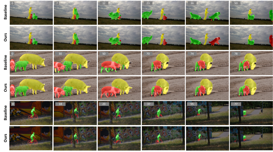
Figure 2: Qualitative results of our method and a baseline (a DeAOTT model with the vanilla attention trained using the standard KD, i.e., only logit layers are transferred). As shown, compared with the baseline, our method can maintain the association of the objects and their IDs across frames (see frame 36 in the 1st and 2nd row). Our method also tends to be aware of parts of the same object (see frame 50 in the 3rd and 4th row). In addition, the object masks generated by our method are well adaptive to temporal changes (see frames 23 and 37 in the 5th and 6th row). We hypothesize this success is due to the cross-frame adaptivity of deformable attention over its counterpart. More results are provided in our supplementary material.

4.3 Evaluation and results

We first evaluate our proposed deformable attention in learning of attention maps in VOS. To do this, we experiment our framework (in Figure 1(a)) with the vanilla attention and deformable attention. We report the results of this experiment in Table 1. As shown in the results, the deformable attention outperforms the vanilla one on all the evaluation metrics and across all the datasets.

Next, we evaluate the effectiveness of our proposed KD method. Recall that our method also distills the attention maps, in addition to the logits during the distillation process. Therefore, to validate this idea, we compare our KD strategy with the one in [19], which transfers only the logits from the teacher to the student model. This strategy is equivalent to setting $\lambda$ (in Eq. 12) to 0. In addition, we experiment with the state-of-the-art KD algorithm in [6]. For a fair comparison, we replicate the methods in [19, 6] for the VOS scenario using the same experimental setup presented in Section 4.2. We summarise the results of this comparison in Table 2. The experimental results confirm the benefit of distillation of intermediate attention maps during the distillation process. The results also show the superiority of our proposed KD method over the state-of-the-art KD.

We compare our method with existing self-supervised/unsupervised VOS methods on common datasets and present the comparison results in Table 3. In addition to evaluating the methods using segmentation accuracy metrics, we also compare their computational speed using frame-per-second (FPS) metric. As shown in Table 3, our method ranks first on the YouTube-VOS 2018 dataset and second on the DAVIS 2017 in terms of the segmentation accuracy (evident by the $\mathcal{J}\&\mathcal{F}$ scores). However, compared with the first-ranked method, i.e., UnifiedMask [25], although our method incurs a lower accuracy ($<2.5\%$ of the $\mathcal{J}\&\mathcal{F}$ score), it takes much less memory due to the lightweight architecture yet offers a much faster inference speed (about 50 $\times$ of the FPS), making the VOS real-time and feasible to low-powered devices. We summarise the segmentation accuracy vs memory footprint of all the methods in Figure 3. We visualise several qualitative results of our method in Figure 2.

Figure 3: Comparison of self-supervised/unsupervised VOS methods in terms of segmentation accuracy ($\mathcal{J}\&\mathcal{F}$) and memory footprint on DAVIS-17 Val dataset.

Figure 4: Convergence analysis of the loss functions.

4.4 Ablation study

We conducted ablative experiments to explain the rationale behind the design and settings of our method.

Loss functions

Recall that we propose to use the CKA score [21] to define the loss for attention distillation in Eq. 9. We prove that such a selection is effective. Specifically, we compare the CKA with the commonly used KL divergence in implementing the attention distillation loss. We present this comparison in Figure 4. We observe that the CKA loss is well below the KL loss and clearly shows its convergence. This result also illustrates the anisotropic property of the KL loss in KD. We also investigate the logit distillation loss ($\mathcal{L}_{inter}+\mathcal{L}_{inter}$) in Eq. 11 and the entire loss ($\mathcal{L}$) in Eq. 12 in Figure 4. As shown, our loss functions converge during the KD process.

Distillation information

An important question to KD applications is what information should be distilled. In this ablation study, we experiment with different combinations of attention and logit layers used in the distillation process. Specifically, we choose attention maps generated from the GPM of the ID branch from the teacher model (see Figure 1(a)). Recall that our student network is trained by distillation of the attention map and the logit layer in the 3rd GPM from the teacher network. We report the performance of these combinations in Table 4, which clearly confirms the best performance of our student network.

	DAVIS-17 Val
Variant	$\mathcal{J}$&$\mathcal{F}\uparrow$	$\mathcal{J}\uparrow$	$\mathcal{F}\uparrow$
Att. map 1, logit	70.75	68.30	73.20
Att. map 2, logit	70.80	68.45	73.15
Att. map 3, logit	70.95	67.50	74.40
Our student network	72.75	69.90	75.60

Table 4: Performance of different combinations of attention maps and logit layers used in the distillation process. For the first three variants, we used only $\mathcal{L}_{inter}$ and $\mathcal{L}_{att}$ for training. Best performances are highlighted.

5 Conclusion

We propose a novel method for video object segmentation (VOS) with self-supervised learning. The novelty of our work lies in improving attention learning to adapt with temporal changes in VOS via deformable attention that allows flexible feature locating, and a new knowledge distillation framework that enhances the distillation process via attention transfer. We apply these technical innovations to create and train a lightweight VOS network in the self-supervised fashion. The network is shown to be adapted to both the spatial and temporal dimensions. We evaluate our method through extensive experiments on several benchmark datasets. Experimental results verify the robustness and efficiency of our method, achieving state-of-the-art performance and optimal memory usage.

Appendices

Self-supervised Video Object Segmentation with Distillation Learning of Deformable Attention
–Supplementary Material–

Appendix A Network architectures

We refer the reader to Figure 1 in the main paper where we depict the full pipeline of our method. In the following sub-sections, we provide technical details for main components in the pipeline.

A Encoder

We utilised ResNet-50 and MobileNet-V2 as respective teacher’s and student’s backbones. Similarly to DeAOT [51], we modified the MobileNet-V2 encoder to include a dilation in the last stage and removed the stride from the first convolution in this last stage. We also removed the last stage in the ResNet-50 backbone.

B Gated propagation module and gated deformable propagation module

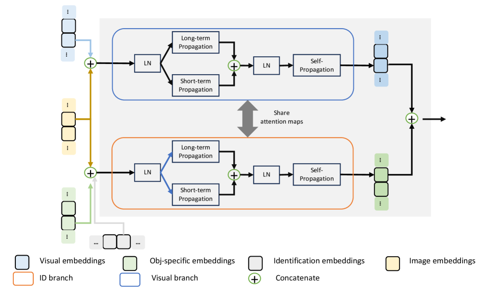
Figure 5: Gated propagation module.

We illustrate the gated propagation module (GPM) in Figure 5. Inputs for the GPM include visual embeddings, object-specific embeddings, identification embeddings and image embeddings. Those embedings are concatenated to be passed through a visual branch and an ID branch, each of which includes a series of long short-term transformers. Specifically, image embeddings are produced by the image encoder, which we present in Section A. Visual embeddings and object-specific embeddings are the results of the visual and ID branch, respectively. Identification embeddings are generated from a decoder with respect to the previous frame. We describe the decoder in Section D. Note that, the visual branch and ID branch share the same attention maps.

The concatenated embedding inputs are fed into a Layer Normalization (LN). Long-term propagation, short-term propagation, and self-propagation modules in Figure 5, are implemented as vanilla attention.

The gated deformable propagation module (GDPM) shares a similar architecture with the GPM. However, we replace the vanilla attention in the long-term propagation and self-propagation in both ID branch and visual branch by our deformable attention.

C Deformable attention

We use single-head deformable attention in our student network to lighten the network architecture while ensuring the quality of object segmentation.

Our deformable attention offers flexible locations for the key and value via an offset network. The offset network consists of 2 convolutional layers with GELU activation functions in between (please refer to Figure 1(c) in the main paper). The query $Q\in\mathbb{R}^{H\times W\times C_{Q}}$ fed into the offset network is calculated by a linear transformation as $Q=W_{q}X$ and partitioned uniformly along its feature channels into $S$ groups, resulting sub-feature maps $\left\{Q_{i}\in\mathbb{R}^{H\times W\times C_{Q_{i}}}\right\}_{i=1}^{S}$. We set $C_{Q}=512$ and $S=4$. The partition of $Q$ into smaller groups in the first convolution aims at controlling the connections between input feature channels and output channels. This convolution has kernel size of 5, stride of 1, padding of 2. The dimensions for the input and output channels are set to $\frac{C_{Q_{i}}}{S}$.

For the second convolutional layer, $1\times 1$ convolution is applied. The resulting offsets $\Delta\in\mathbb{R}^{2\times S\times H_{g}\times W_{g}}$ contain the offset values for both vertical and horizontal directions with respect to reference points. These offsets are then used to shift the reference points for locating the deformable key $\tilde{K}$ and value $\tilde{V}$, which are finally used to calculate a deformable attention map.

Figure 6: Decoder architecture. We utilised a feature pyramid network to make our decoder.

D Decoder

Figure 6 provides an overview of the decoder used in our paper. Inputs for the decoder are visual and object-specific embeddings, which are reshaped into 2D-forms before being passed into the decoder. The decoder includes a series of convolutional layers with skip connections and bilinear upsampling layers. The final convolutional layer returns logits, which are then converted into a segmentation mask.

	DAVIS-16 Val			DAVIS-17 Val			YT-VOS18	YT-VOS19
Loss function	$\mathcal{J}$&$\mathcal{F}\uparrow$	$\mathcal{J}\uparrow$	$\mathcal{F}\uparrow$	$\mathcal{J}$&$\mathcal{F}\uparrow$	$\mathcal{J}\uparrow$	$\mathcal{F}\uparrow$	$\mathcal{J}$&$\mathcal{F}\uparrow$	$\mathcal{J}$&$\mathcal{F}\uparrow$
$\mathcal{L}_{inter}$	83.50	82.70	84.30	68.75	66.20	71.30	69.83	71.05
$\mathcal{L}_{inter}+\mathcal{L}_{intra}$	82.50	82.10	83.50	69.50	66.90	72.10	69.67	70.94
$\mathcal{L}_{inter}+\mathcal{L}_{intra}+\lambda\mathcal{L}_{att}$	85.75	84.90	86.60	72.75	69.90	75.60	73.18	73.95

Table 5: Comparison of loss functions. Best performances are highlighted.

	DAVIS-16 Val			DAVIS-17 Val			YT-VOS18	YT-VOS19
Value for $\lambda$	$\mathcal{J}$&$\mathcal{F}\uparrow$	$\mathcal{J}\uparrow$	$\mathcal{F}\uparrow$	$\mathcal{J}$&$\mathcal{F}\uparrow$	$\mathcal{J}\uparrow$	$\mathcal{F}\uparrow$	$\mathcal{J}$&$\mathcal{F}\uparrow$	$\mathcal{J}$&$\mathcal{F}\uparrow$
$\lambda=0.5$	83.75	83.2	84.3	68.25	65.6	70.9	69.35	70.93
$\lambda=1.0$	83.55	83	84.1	69.1	66.7	71.5	68.23	69.47
$\lambda=1.5$	85.75	84.90	86.60	72.75	69.90	75.60	73.18	73.95
$\lambda=2.0$	81.60	81.20	82.00	64.75	63.10	66.40	69.90	67.17

Table 6: Parameter setting for $\lambda$. Best performances are highlighted.

Appendix B Quantitative evaluation

A Loss functions

In our ablation study (section 4.4) in the main paper, we study the impact of the loss functions by investigating their convergence during training (please see the learning curves in Fig. 4 in the main paper). Here, we verify their role in testing. In particular, we measure the $\mathcal{J}$, $\mathcal{F}$, and $\mathcal{J}\&\mathcal{F}$ scores of different combinations of the loss functions on the test sets. We report the results of this experiment in Table 5. As shown in the results, our defined loss, combining all $\mathcal{L}_{inter}$, $\mathcal{L}_{intra}$, and $\mathcal{L}_{att}$ achieves the best performance on all evaluation metrics across all datasets.

B Balance factor $\lambda$

Recall that our distillation loss is defined as,

$$\mathcal{L}=\mathcal{L}_{inter}+\mathcal{L}_{intra}+\lambda\mathcal{L}_{att}$$

where $\lambda$ is a user-defined paramter to balance the logit and attention losses.

We experiment $\lambda$ with various values. Experimental results (in Table 6) show that our current setting ($\lambda=1.5$) achieves the best performance.

C Distance metrics

In Figure 4 in the main paper, we analyse the convergence of the attention loss $\mathcal{L}_{att}$ using CKA and KL-divergence metrics. Here, we quantitatively evaluate these distance metrics in terms of the performance of VOS. We report the results of this study in Table 7, which clearly confirms our choice (i.e., CKA) for the attention loss.

	DAVIS-17 Val
Variant	$\mathcal{J}$&$\mathcal{F}\uparrow$	$\mathcal{J}\uparrow$	$\mathcal{F}\uparrow$
KL-divergence	54.65	52.10	57.20
CKA	72.75	69.90	75.60

Table 7: Comparison of KL-divergence and CKA. Best performances are highlighted.

	DAVIS-17 Val
Variant	$\mathcal{J}$&$\mathcal{F}\uparrow$	$\mathcal{J}\uparrow$	$\mathcal{F}\uparrow$
Att. map 1, logit	69.65	66.90	72.40
Att. map 2, logit	66.40	63.80	69.00
Att. map 3, logit	72.75	69.90	75.60

Table 8: Comparison of different combinations of attention maps and logit layers used in the distillation process. Our student network distills the attention map and logit layer in the 3rd Gated Propagation Module from the teacher network. Best performances are highlighted.

D Information selection for distillation

In Table 4 in the main paper, we evaluate different combinations of attention maps and logit layers used in the distillation process. However, we use only $\mathcal{L}_{inter}$ and $\mathcal{L}_{att}$ in the main paper to show the necessity of distillation of attention maps. Here, we test these combinations using our full loss, defined in Eq. (12) in the main paper. We present the results of this experiment in Table 8. As shown, these results are consistent with those presented in Table 4 in the main. This means that our current setting (combination of attention map 3 and logit layer) makes the best setting.

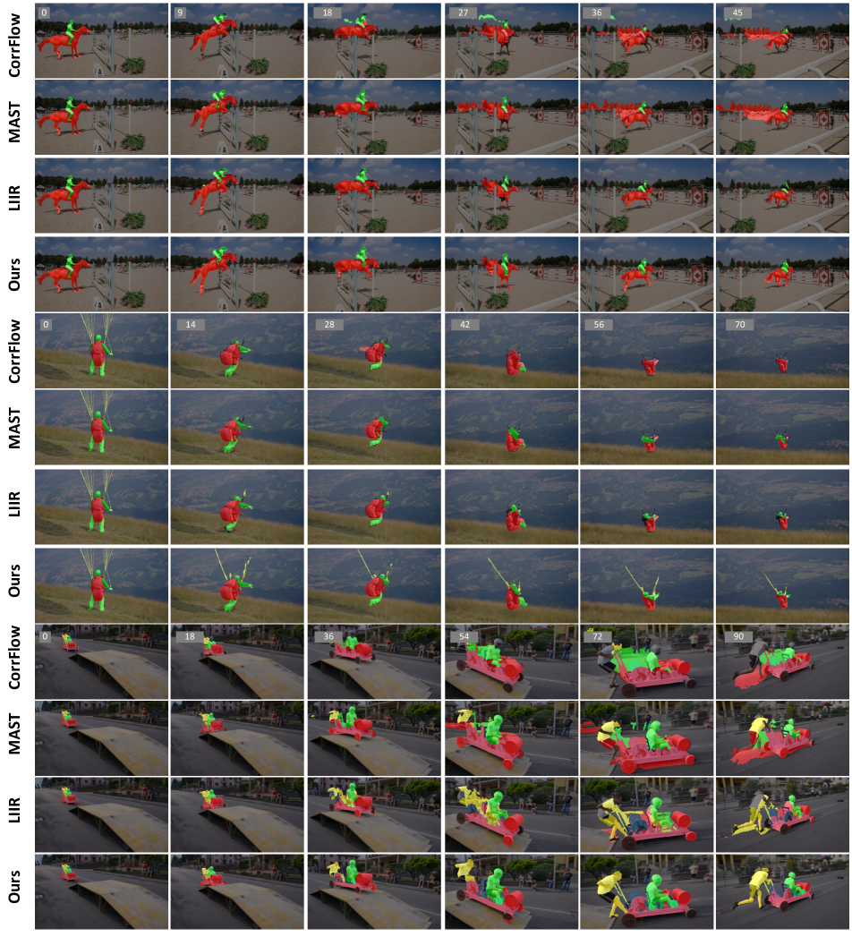
Figure 7: Qualitative comparison of our method with existing ones on the DAVIS2017 Val dataset [37]. As shown, our method clearly provides better segmentation results, compared with existing ones.

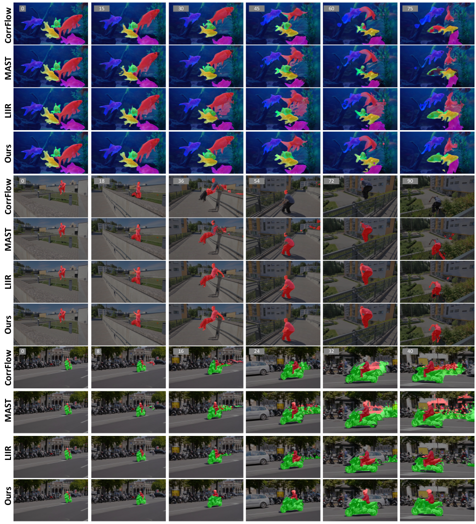
Figure 8: Other qualitative results on the DAVIS2017 Val dataset [37]. Compared with other methods, our method still shows more advanced in challenging cases, e.g., high deformation (1st - 4th rows), fast motion (5th - 8th rows), and cluttered background (9th - 12th rows).

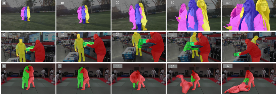
Figure 9: Limitations of our method. These qualitative results on the DAVIS2017 Val dataset [37] show that our method fails to segment objects under moving cameras and intra-target scale variation (1st row), out-of-plane rotation (2nd and 3rd rows). Intra-target scale variation means the target object changes its scale significantly by suddenly moving closer/further from the camera.

Appendix C Qualitative evaluation

We provide qualitative comparisons of our method with existing ones including CorrFlow [22], MAST [23], LIIR [24] in Figure 7 and Figure  8. We also present several fail cases of our method in Figure  9.

Figure 7 and Figure  8 show challenging cases with high deformation, fast moving and cluttered background. Figure 9 demonstrates limitations of our method. As shown, our method struggles with videos containing out-of-plane rotation and intra-target scale variation. Intra-target scale variation means the target object changes its scale significantly by suddenly moving closer/further from the camera.

References

- Ainslie et al. [2020] Joshua Ainslie, Santiago Ontanon, Chris Alberti, Vaclav Cvicek, Zachary Fisher, Philip Pham, Anirudh Ravula, Sumit Sanghai, Qifan Wang, and Li Yang. ETC: Encoding long and structured inputs in transformers. arXiv preprint arXiv:2004.08483, 2020.
- Brown et al. [2020] Tom Brown, Benjamin Mann, Nick Ryder, Melanie Subbiah, Jared D Kaplan, Prafulla Dhariwal, Arvind Neelakantan, Pranav Shyam, Girish Sastry, Amanda Askell, et al. Language models are few-shot learners. Neural Information Processing systems, 33:1877–1901, 2020.
- Caelles et al. [2017] Sergi Caelles, Kevis-Kokitsi Maninis, Jordi Pont-Tuset, Laura Leal-Taixé, Daniel Cremers, and Luc Van Gool. One-shot video object segmentation. In IEEE/CVF Conference on Computer Vision and Pattern Recognition, pages 221–230, 2017.
- Carion et al. [2020] Nicolas Carion, Francisco Massa, Gabriel Synnaeve, Nicolas Usunier, Alexander Kirillov, and Sergey Zagoruyko. End-to-end object detection with transformers. In European Conference on Computer Vision, pages 213–229, 2020.
- Chen et al. [2020] Mark Chen, Alec Radford, Rewon Child, Jeffrey Wu, Heewoo Jun, David Luan, and Ilya Sutskever. Generative pretraining from pixels. In International Conference on Machine Learning, pages 1691–1703, 2020.
- Chen et al. [2022] Yudong Chen, Sen Wang, Jiajun Liu, Xuwei Xu, Frank de Hoog, and Zi Huang. Improved feature distillation via projector ensemble. In Neural Information Processing Systems, pages 12084–12095, 2022.
- Cheng et al. [2020] Ho Kei Cheng, Jihoon Chung, Yu-Wing Tai, and Chi-Keung Tang. Cascadepsp: Toward class-agnostic and very high-resolution segmentation via global and local refinement. In Proceedings of the IEEE/CVF Conference on Computer Vision and Pattern Recognition, pages 8890–8899, 2020.
- Cheng et al. [2021a] Ho Kei Cheng, Yu-Wing Tai, and Chi-Keung Tang. Modular interactive video object segmentation: Interaction-to-mask, propagation and difference-aware fusion. In IEEE/CVF Conference on Computer Vision and Pattern Recognition, pages 5559–5568, 2021a.
- Cheng et al. [2021b] Ho Kei Cheng, Yu-Wing Tai, and Chi-Keung Tang. Rethinking space-time networks with improved memory coverage for efficient video object segmentation. In Neural Information Processing Systems, pages 11781–11794, 2021b.
- Cheng et al. [2023] Tianheng Cheng, Xinggang Wang, Shaoyu Chen, Qian Zhang, and Wenyu Liu. Boxteacher: Exploring high-quality pseudo labels for weakly supervised instance segmentation. In IEEE/CVF Conference on Computer Vision and Pattern Recognition, pages 3145–3154, 2023.
- Dai et al. [2017] Jifeng Dai, Haozhi Qi, Yuwen Xiong, Yi Li, Guodong Zhang, Han Hu, and Yichen Wei. Deformable convolutional networks. In IEEE/CVF International Conference on Computer Vision, pages 764–773, 2017.
- Dong et al. [2022] Xiaoyi Dong, Jianmin Bao, Dongdong Chen, Weiming Zhang, Nenghai Yu, Lu Yuan, Dong Chen, and Baining Guo. Cswin transformer: A general vision transformer backbone with cross-shaped windows. In IEEE/CVF Conference on Computer Vision and Pattern Recognition, pages 12124–12134, 2022.
- Dosovitskiy et al. [2021] Alexey Dosovitskiy, Lucas Beyer, Alexander Kolesnikov, Dirk Weissenborn, Xiaohua Zhai, Thomas Unterthiner, Mostafa Dehghani, Matthias Minderer, Georg Heigold, Sylvain Gelly, et al. An image is worth 16x16 words: Transformers for image recognition at scale. In International Conference on Learning Representation, 2021.
- Duke et al. [2021] Brendan Duke, Abdalla Ahmed, Christian Wolf, Parham Aarabi, and Graham W. Taylor. SSTVOS: sparse spatiotemporal transformers for video object segmentation. In IEEE/CVF Conference on Computer Vision and Pattern Recognition, pages 5912–5921, 2021.
- Gao et al. [2023] Mingqi Gao, Feng Zheng, James J. Q. Yu, Caifeng Shan, Guiguang Ding, and Jungong Han. Deep learning for video object segmentation: a review. Artificial Intelligence Review, 56(1):457–531, 2023.
- Gretton et al. [2005] Arthur Gretton, Olivier Bousquet, Alex Smola, and Bernhard Schölkopf. Measuring statistical dependence with hilbert-schmidt norms. In International Conference on Algorithmic Learning Theory, pages 63–77, 2005.
- Heo et al. [2022] Miran Heo, Sukjun Hwang, Seoung Wug Oh, Joon-Young Lee, and Seon Joo Kim. VITA: video instance segmentation via object token association. In Neural Information Processing Systems, 2022.
- Hu et al. [2018] Ping Hu, Gang Wang, Xiangfei Kong, Jason Kuen, and Yap-Peng Tan. Motion-guided cascaded refinement network for video object segmentation. In IEEE/CVF Conference on Computer Vision and Pattern Recognition, pages 1400–1409, 2018.
- Huang et al. [2022] Tao Huang, Shan You, Fei Wang, Chen Qian, and Chang Xu. Knowledge distillation from a stronger teacher. In Neural Information Processing Systems, pages 33716–33727, 2022.
- Jeon et al. [2021] Sangryul Jeon, Dongbo Min, Seungryong Kim, and Kwanghoon Sohn. Mining better samples for contrastive learning of temporal correspondence. In Proceedings of the IEEE/CVF Conference on Computer Vision and Pattern Recognition, pages 1034–1044, 2021.
- Kornblith et al. [2019] Simon Kornblith, Mohammad Norouzi, Honglak Lee, and Geoffrey Hinton. Similarity of neural network representations revisited. In International Conference on Machine Learning, pages 3519–3529, 2019.
- Lai and Xie [2019] Z. Lai and W. Xie. Self-supervised learning for video correspondence flow. In BMVC, 2019.
- Lai et al. [2020] Zihang Lai, Erika Lu, and Weidi Xie. Mast: A memory-augmented self-supervised tracker. In Proceedings of the IEEE/CVF Conference on Computer Vision and Pattern Recognition, pages 6479–6488, 2020.
- Li et al. [2022] Liulei Li, Tianfei Zhou, Wenguan Wang, Lu Yang, Jianwu Li, and Yi Yang. Locality-aware inter-and intra-video reconstruction for self-supervised correspondence learning. In Proceedings of the IEEE/CVF Conference on Computer Vision and Pattern Recognition, pages 8719–8730, 2022.
- Li et al. [2023] Liulei Li, Wenguan Wang, Tianfei Zhou, Jianwu Li, and Yi Yang. Unified mask embedding and correspondence learning for self-supervised video segmentation. In Proceedings of the IEEE/CVF Conference on Computer Vision and Pattern Recognition, pages 18706–18716, 2023.
- Li and Loy [2018] Xiaoxiao Li and Chen Change Loy. Video object segmentation with joint re-identification and attention-aware mask propagation. In European Conference on Computer Vision, pages 90–105, 2018.
- Li et al. [2020] Xiang Li, Tianhan Wei, Yau Pun Chen, Yu-Wing Tai, and Chi-Keung Tang. Fss-1000: A 1000-class dataset for few-shot segmentation. In Proceedings of the IEEE/CVF conference on computer vision and pattern recognition, pages 2869–2878, 2020.
- Liu et al. [2023] Dongyang Liu, Meina Kan, Shiguang Shan, and Xilin Chen. Function-consistent feature distillation. International Conference on Learning Representations, 2023.
- Liu et al. [2021] Ze Liu, Yutong Lin, Yue Cao, Han Hu, Yixuan Wei, Zheng Zhang, Stephen Lin, and Baining Guo. Swin transformer: Hierarchical vision transformer using shifted windows. In IEEE/CVF International Conference on Computer Vision, pages 10012–10022, 2021.
- Miao et al. [2020] Jiaxu Miao, Yunchao Wei, and Yi Yang. Memory aggregation networks for efficient interactive video object segmentation. In IEEE/CVF Conference on Computer Vision and Pattern Recognition, pages 10363–10372, 2020.
- Miles et al. [2023] Roy Miles, Mehmet Kerim Yucel, Bruno Manganelli, and Albert Saà-Garriga. MobileVOS: Real-time video object segmentation contrastive learning meets knowledge distillation. In IEEE/CVF Conference on Computer Vision and Pattern Recognition, pages 10480–10490, 2023.
- Pan et al. [2023] Xuran Pan, Tianzhu Ye, Zhuofan Xia, Shiji Song, and Gao Huang. Slide-transformer: Hierarchical vision transformer with local self-attention. In IEEE/CVF Conference on Computer Vision and Pattern Recognition, pages 2082–2091, 2023.
- Park et al. [2021] Dae Young Park, Moon-Hyun Cha, Daesin Kim, Bohyung Han, et al. Learning student-friendly teacher networks for knowledge distillation. In Neural Information Processing Systems, pages 13292–13303, 2021.
- Park et al. [2022] Kwanyong Park, Sanghyun Woo, Seoung Wug Oh, In So Kweon, and Joon-Young Lee. Per-clip video object segmentation. In IEEE/CVF Conference on Computer Vision and Pattern Recognition, pages 1352–1361, 2022.
- Perazzi et al. [2016] Federico Perazzi, Jordi Pont-Tuset, Brian McWilliams, Luc Van Gool, Markus Gross, and Alexander Sorkine-Hornung. A benchmark dataset and evaluation methodology for video object segmentation. In IEEE/CVF Conference on Computer Vision and Pattern Recognition, pages 724–732, 2016.
- Perazzi et al. [2017] Federico Perazzi, Anna Khoreva, Rodrigo Benenson, Bernt Schiele, and Alexander Sorkine-Hornung. Learning video object segmentation from static images. In IEEE/CVF Conference on Computer Vision and Pattern Recognition, pages 2663–2672, 2017.
- Pont-Tuset et al. [2017] Jordi Pont-Tuset, Federico Perazzi, Sergi Caelles, Pablo Arbeláez, Alex Sorkine-Hornung, and Luc Van Gool. The 2017 davis challenge on video object segmentation. arXiv preprint arXiv:1704.00675, 2017.
- Radford et al. [2021] Alec Radford, Jong Wook Kim, Chris Hallacy, Aditya Ramesh, Gabriel Goh, Sandhini Agarwal, Girish Sastry, Amanda Askell, Pamela Mishkin, Jack Clark, et al. Learning transferable visual models from natural language supervision. In International Conference on Machine Learning, pages 8748–8763, 2021.
- Ramachandran et al. [2017] Prajit Ramachandran, Barret Zoph, and Quoc V Le. Searching for activation functions. arXiv preprint arXiv:1710.05941, 2017.
- Richter and Pal [2022] Mats L Richter and Christopher Pal. Receptive field refinement for convolutional neural networks reliably improves predictive performance. arXiv preprint arXiv:2211.14487, 2022.
- Shi et al. [2015] Jianping Shi, Qiong Yan, Li Xu, and Jiaya Jia. Hierarchical image saliency detection on extended cssd. IEEE transactions on pattern analysis and machine intelligence, 38(4):717–729, 2015.
- Son [2022] Jeany Son. Contrastive learning for space-time correspondence via self-cycle consistency. In Proceedings of the IEEE/CVF Conference on Computer Vision and Pattern Recognition, pages 14679–14688, 2022.
- Strudel et al. [2021] Robin Strudel, Ricardo Garcia, Ivan Laptev, and Cordelia Schmid. Segmenter: Transformer for semantic segmentation. In IEEE/CVF International Conference on Computer Vision, pages 7262–7272, 2021.
- Tsai et al. [2016] Yi-Hsuan Tsai, Ming-Hsuan Yang, and Michael J Black. Video segmentation via object flow. In IEEE/CVF Conference on Computer Vision and Pattern Recognition, pages 3899–3908, 2016.
- Vaswani et al. [2017] Ashish Vaswani, Noam Shazeer, Niki Parmar, Jakob Uszkoreit, Llion Jones, Aidan N. Gomez, Lukasz Kaiser, and Illia Polosukhin. Attention is all you need. In Proceedings of the Advances in Neural Information Processing Systems, pages 5998–6008, 2017.
- Wang et al. [2017] Lijun Wang, Huchuan Lu, Yifan Wang, Mengyang Feng, Dong Wang, Baocai Yin, and Xiang Ruan. Learning to detect salient objects with image-level supervision. In Proceedings of the IEEE conference on computer vision and pattern recognition, pages 136–145, 2017.
- Xia et al. [2022] Zhuofan Xia, Xuran Pan, Shiji Song, Li Erran Li, and Gao Huang. Vision transformer with deformable attention. In IEEE/CVF Conference on Computer Vision and Pattern Recognition, pages 4794–4803, 2022.
- Xiao et al. [2021] Tete Xiao, Mannat Singh, Eric Mintun, Trevor Darrell, Piotr Dollár, and Ross Girshick. Early convolutions help transformers see better. In Neural Information Processing Systems, pages 30392–30400, 2021.
- Xu et al. [2023] Mengde Xu, Zheng Zhang, Fangyun Wei, Han Hu, and Xiang Bai. Side adapter network for open-vocabulary semantic segmentation. In IEEE/CVF Conference on Computer Vision and Pattern Recognition, pages 2945–2954, 2023.
- Xu et al. [2018] Ning Xu, Linjie Yang, Yuchen Fan, Dingcheng Yue, Yuchen Liang, Jianchao Yang, and Thomas Huang. Youtube-vos: A large-scale video object segmentation benchmark. arXiv preprint arXiv:1809.03327, 2018.
- Yang and Yang [2022] Zongxin Yang and Yi Yang. Decoupling features in hierarchical propagation for video object segmentation. In Neural Information Processing Systems, 2022.
- Yang et al. [2021] Zongxin Yang, Yunchao Wei, and Yi Yang. Associating objects with transformers for video object segmentation. In Neural Information Processing Systems, pages 2491–2502, 2021.
- Yoo et al. [2023] Jun-Sang Yoo, Hongjae Lee, and Seung-Won Jung. Hierarchical spatiotemporal transformers for video object segmentation. arXiv preprint arXiv:2307.08263, 2023.
- Yu et al. [2022] Ye Yu, Jialin Yuan, Gaurav Mittal, Li Fuxin, and Mei Chen. Batman: Bilateral attention transformer in motion-appearance neighboring space for video object segmentation. In European Conference on Computer Vision, pages 612–629, 2022.
- Zeng et al. [2019] Yi Zeng, Pingping Zhang, Jianming Zhang, Zhe Lin, and Huchuan Lu. Towards high-resolution salient object detection. In Proceedings of the IEEE/CVF international conference on computer vision, pages 7234–7243, 2019.
- Zhang et al. [2023] Yurong Zhang, Liulei Li, Wenguan Wang, Rong Xie, Li Song, and Wenjun Zhang. Boosting video object segmentation via space-time correspondence learning. In IEEE/CVF Conference on Computer Vision and Pattern Recognition, pages 2246–2256, 2023.
- Zong et al. [2022] Martin Zong, Zengyu Qiu, Xinzhu Ma, Kunlin Yang, Chunya Liu, Jun Hou, Shuai Yi, and Wanli Ouyang. Better teacher better student: Dynamic prior knowledge for knowledge distillation. In International Conference on Learning Representations, 2022.