Learning-based Sensing and Computing Decision
for Data Freshness
in Edge Computing-enabled Networks

Abstract

As the demand on artificial intelligence (AI)-based applications increases, the freshness of sensed data becomes crucial in the wireless sensor networks. Since those applications require a large amount of computation for processing the sensed data, it is essential to offload the computation load to the edge computing (EC) server. In this paper, we propose the sensing and computing decision (SCD) algorithms for data freshness in the EC-enabled wireless sensor networks. We define the $\eta$-coverage probability to show the probability of maintaining fresh data for more than $\eta$ ratio of the network, where the spatial-temporal correlation of information is considered. We then propose the probability-based SCD for the single pre-charged sensor case with providing the optimal point after deriving the $\eta$-coverage probability. We also propose the reinforcement learning (RL)-based SCD by training the SCD policy of sensors for both the single pre-charged and multiple energy harvesting (EH) sensor cases, to make a real-time decision based on its observation. Our simulation results verify the performance of the proposed algorithms under various environment settings, and show that the RL-based SCD algorithm achieves higher performance compared to baseline algorithms for both the single pre-charged sensor and multiple EH sensor cases.

I Introduction

The new generation of wireless networks will realize the intelligence of everything, which integrates the digital world and the physical world by sensing everything [2]. This will lead to the change on the role of wireless sensor networks (WSN) from providing sensed data efficiently to providing fresh data reliably. The data freshness is especially crucial for AI-based decision making applications and services such as the autonomous driving and the security surveillance [3]. In those services, the outdated information can cause the fatal problems such as the car accident or the invasion. For maintaining the data freshness in the sensor networks, the sensor should be continuously activated and transmit the sensed data to the sink node that manages the data. However, because of the limited battery capacity of sensors, frequent sensing and transmission may shorten the sensor lifetime and fail to maintain the data freshness in the networks. Hence, both the energy consumption and the data freshness should be considered in the design of sensor networks.

Furthermore, as the demand on AI-based applications and services is increasing, the processing of the sensed data requires a larger amount of computation. The large computation might not be able to be done at the sensors due to the large energy consumption as well as the long processing delay from the low computing capability of sensors. Hence, the EC, which is to offload the computation load of sensors to the EC server, becomes essential for energy-efficient wireless sensor networks [4, 5].

Recently, the data freshness has been considered in many works for the energy-efficient sensor networks[6, 7, 8, 9, 10, 11, 12, 13, 14]. Here, to measure the data freshness, the age of information (AoI) has been used, which is the elapsed time since the generation of the data[15]. For the single sensor case, the average AoI [7] and the probability mass function (PMF) of AoI [6] are studied for given sensing decision period. The sensing decision algorithms are presented to minimize the average AoI of the single sensor using the threshold-based [8, 9] and the RL-based approach [10]. By considering multiple sensors, the average AoI is analyzed in [11], when the sensing instances are determined randomly and independently with the exponentially-distributed intervals. The sensing decision algorithms are also presented to minimize the average AoI of sensors using the Lyapunov optimization and the RL-based approach[12]. However, in those works, the EC is not considered in the design of the sensor networks.

The EC-enabled sensor networks have been introduced in recent works [16, 17]. In those works, the computing decision has been studied to determine whether the sensor computes the task locally or offloads it to the EC server. Specifically, for multiple sensor case, the computing decision algorithms are presented to minimize the latency and the computing energy consumption using the convex optimization-based [16] and the game theory-based approach [17]. Recently, in [18], the data freshness is also considered in the computing decision algorithm, which is designed to minimize the weighted sum of computing delay and energy consumption with guaranteeing the data freshness constraint. As such, most existing studies are focused on either sensing or computing decision. Nevertheless, since both the sensing decision and computing decision affect the performance of the wireless sensor networks, they should be jointly designed.

The joint SCD has been designed for data freshness in [19, 20]. For the single sensor case, the RL-based SCD algorithm is proposed to minimize the average AoI. Moreover, for the multiple sensor case, the Lyapunov optimization-based SCD algorithm is presented to minimize the peak AoI. Generally, the sensed data has a temporal correlation, which means it can be similar to the data, sensed in a short time ago [21]. Furthermore, in the wireless sensor networks, where sensors are densely deployed, the sensing coverage of nearby sensors can have overlapping areas, which means the sensed data from the sensors can have a spatial correlation as well [22]. Those correlation affect the accuracy of the sensed data, which decreases over time and as the distance to the sensing point increases [13]. Therefore, in the energy-efficient design of the SCD for the multiple sensor case, the temporal and the spatial correlation of sensed data should be jointly considered, but in [19, 20], only the temporal correlation is considered.

Thus, in this paper, we propose the SCD algorithms for data freshness in the EC-enabled wireless sensor networks by considering the spatial-temporal correlation of information. Specifically, we consider that the information at different locations, estimated from the sensed data, has the error, which increases with the distance from the sensor and the elapsed time from sensing. Therefore, we define the error-tolerable network coverage ratio as the portion of network area with smaller error than certain threshold. We then propose the $\eta$-coverage probability as a performance metric, which is the probability that the network coverage ratio is greater than the target value $\eta$. To maximize the $\eta$-coverage probability, we propose the SCD algorithms for two cases: the single pre-charged sensor case and the multiple EH sensor case, respectively. We first propose the probability-based SCD algorithm, where each sensor makes a decision based on the sensing and EC probabilities. Next, we propose the RL-based SCD algorithm, where each sensor takes an action based on the real-time information as an observation. The main contributions of this paper can be summarized as follows.

• We propose the SCD algorithms for data freshness in the EC-enabled wireless sensor networks. To the best of our knowledge, this is the first work that jointly decides the sensing and computation considering both the spatial and the temporal correlation.

• In the probability-based SCD algorithm, we derive the $\eta$-coverage probability and provide the optimal sensing probability that maximizes the $\eta$-coverage probability in a closed form for the single pre-charged sensor case. We also provide the method to obtain the optimal sensing and EC probabilities for the multiple EH sensor case.

• In the RL-based SCD algorithm, we train the policy for each sensor to make the SCD according to the dynamic change of environments including the battery level of the sensors and the channel fading gain for the multiple EH sensor case as well as the single pre-charged sensor case.

• In simulation results, we verify the $\eta$-coverage probability of the proposed algorithms for various environment settings such as the target network coverage ratio, the distance between the sensor and the sink node, the number of sensors, and the computing energy.

Figure 1: Network description of EC-enabled wireless sensor networks.

The remainder of this paper is outlined as follows. In Section II, we firstly describe the EC-enabled wireless sensor networks model, and define the $\eta$-coverage probability as a performance metric by introducing the AoI. To maximize the $\eta$-coverage probability for both the single pre-charged and the multiple EH sensor cases, we propose two algorithms, the probability-based SCD in Section III and the RL-based SCD in Section IV. In Section V, the simulation results are presented and compared with baselines. Finally, the conclusion of this paper is given in Section VI.

II Edge Computing-enabled Wireless Sensor Networks Model

In this section, we describe the EC-enabled wireless sensor networks model with the transmission and energy models of the networks. After that, we define the $\eta$-coverage probability by introducing the AoI.

II-A Network Description

We consider the EC-enabled wireless sensor networks, operating in a time-slotted fashion, which are composed of sink nodes distributed according to a homogeneous Poisson point process (PPP) with intensity $\lambda$. Each sink node equipped with the EC server is associated with nearby $N_{\text{s}}$ sensors and collects the data from them. An example of the sink node and the associated sensors is given in Fig. 1. We use $\mathcal{N}=\{1,2,\cdots,N_{\text{s}}\}$ as the index set of sensors associated with the sink node, and they have limited battery capacity.

Each sensor makes the SCD at the beginning of each round, which consists of $\tau_{\text{r}}$ time slots. If the sensor performs sensing, it collects the data with size $L_{\text{e}}$ from the surrounding area (e.g., temperature and humidity) for one time slot with consuming the energy $E_{\mathrm{S}}$. Then, the sensed data needs to be computed and transmitted to the sink node. Both the sensors and the EC server have computing capability, so the sensed data can be locally computed at the sensor, i.e., local computing (LC), or offloaded to the EC server, i.e., EC. If the sensor chooses the LC, the data is processed at the sensor for $\tau_{\ell}$ time slots with consuming the energy $E_{\text{C}}$, and it is transmitted to the sink node and the status of the sensor is updated. On the other hand, if the sensor chooses the EC, the data is transmitted to the sink node and computed at the EC server. When the newly sensed data of a sensor arrives at the EC server, but the pre-generated old data of the corresponding sensor still exists at the queue, the old data is replaced with the fresh data. After the EC server processes the data of the sensor for $\tau_{\text{e}}$ time slots, the status of the sensor is updated. Generally, the computing capability of EC server is higher than that of the sensor, so $\tau_{\text{e}}<\tau_{\ell}$. Note that after the computation, the data size reduces to $L_{\ell}$ where $L_{\ell}<L_{\text{e}}$.

II-B Transmission Model

The $n$-th sensor located at $\textbf{x}_{n}$ transmits the data with the transmission power $P_{\text{tx}}$ to the sink node, located at o, with consuming the energy $E_{\mathrm{T}}$. When the sink node receives the sensed data from the $n$-th sensor, the signal-to-interference-plus-noise ratio (SINR) $\zeta_{\textbf{x}_{n},\text{o}}$ is given by

$$\zeta_{\textbf{x}_{n},\text{o}}=\frac{P_{\text{tx}}h_{\textbf{x}_{n},\text{o}}d_{\textbf{x}_{n},\text{o}}^{-\alpha}}{\sigma^{2}+I_{n}},$$ (1)

where $h_{\textbf{x}_{n},\text{o}}$ is the channel fading gain, $d_{\textbf{x}_{n},\text{o}}$ is the distance between the $n$-th sensor and the sink node, $\alpha$ is the path loss exponent, $\sigma^{2}$ is the Additive White Gaussian Noise (AWGN) power. In (1), $I_{n}$ is the inter-cell interference. Each sink node has one sensor that uses the same frequency band with the $n$-th sensor [25]. The distribution of interfering sensors does not constitute a homogeneous PPP due to the dependency of their locations to the sink nodes, but it is shown that this dependency is weak [26]. Hence, we assume the distribution of sensors interfering the $n$-th sensor follows a PPP with intensity $\lambda$. When the probability of using the same frequency resource in other sink nodes for sensors is $p_{\text{t}}$, the density of interfering nodes becomes $\lambda_{\text{I}}=\lambda p_{\text{t}}$, and their distribution is a PPP from the thinning property [27]. Therefore, the inter-cell interference, $I_{n}$, is given by

$$I_{n}=\sum_{\textbf{x}^{\prime}\in\Psi_{n^{\prime}}}P_{\text{tx}}h_{\textbf{x}^{\prime},o}d_{\textbf{x}^{\prime},o}^{-\alpha},$$ (2)

where $\Psi_{n^{\prime}}$ is the location of sensors that use the same frequency resource with the $n$-th sensor.

The transmission can be successful if the data rate is larger than the target data rate. When the Rayleigh fading channel is considered, i.e., $h_{\textbf{x}_{n},\text{o}}\sim\text{exp}(1)$, for the $k$-th data transmission, the outage probability can be given by [28]

$$\begin{aligned} p_{\textbf{o},{k}}&=\mathbb{P}[W\log_{2}(1+\zeta_{\textbf{x}_{n},\text{o}})<R_{m_{k}}]\\ &=\mathbb{E}_{I_{n}}\left[\mathbb{P}\left[h_{\textbf{x}_{n},\text{o}}<\frac{d_{\textbf{x}_{n},\text{o}}^{\alpha}(\sigma^{2}+I_{n})(2^{\frac{R_{m_{k}}}{W}}-1)}{P_{\text{tx}}}\right]\right]\\ &=1-\exp\left(-A\sigma^{2}\right)\mathcal{L}_{I_{n}}\left({A}\right),\end{aligned}$$ (3)

where $m_{k}$ indicates the computing decision, i.e., $m_{k}=\text{e}$ for EC or $m_{k}=\ell$ for LC, $W$ is the bandwidth, and $A=(2^{R_{m_{k}}/W}-1)d_{\textbf{x}_{n},\text{o}}^{\alpha}/P_{\text{tx}}$. Here, $R_{m_{k}}$ is the target data rate that a sensor needs to transmit within time duration $\tau_{\text{t}}$ (i.e., a time slot) [29], so $R_{\text{e}}=L_{\text{e}}/\tau_{\text{t}}$ and $R_{\ell}=L_{\ell}/\tau_{\text{t}}$. Using the definition of the Laplace transform, we have [23, Eq. 3.21]

$$\begin{aligned} \mathcal{L}_{I_{n}}\left({A}\right)=\mathbb{E}_{I_{n}}\left[e^{-AI_{n}}\right]=\exp\left\{-\pi{\lambda_{\text{I}}}(AP_{\text{tx}})^{\frac{2}{\alpha}}\frac{2\pi}{\alpha\sin(2\pi/\alpha)}\right\}.\end{aligned}$$ (4)

By combining (4) with (3), we get the outage probability as

$$\begin{aligned} p_{\textbf{o},{k}}=1-\exp\left\{-A\sigma^{2}-\pi{\lambda_{\text{I}}}(AP_{\text{tx}})^{\frac{2}{\alpha}}\frac{2\pi}{\alpha\sin(2\pi/\alpha)}\right\}.\end{aligned}$$ (5)

Here, $p_{\textbf{o},{k}}>p_{\textbf{o},{j}}$ where $m_{k}=\text{e}$ and $m_{j}=\ell$ as $R_{\text{e}}>R_{\ell}$ due to $L_{\text{e}}>L_{\ell}$.

To improve the data freshness at the sink node, we adopt a retransmission scheme so that the sensor can transmit the data up to $\delta$ times when the current transmission fails. If the transmission fails for $\delta$ times, the sensor drops the data and becomes idle until it has the new data by sensing to prevent the excessive energy consumption.

II-C Energy Model

In wireless sensor networks, sensors are equipped with the battery instead of receiving power via the wire since the deployment of sensors for wired sensor networks may be infeasible, especially in hostile area. Furthermore, the wireless sensor networks have advantages in terms of the installing and maintaining cost, compared to the wired sensor networks [30].

We consider two battery models, generally considered in wireless sensor networks: pre-charged battery model and EH battery model. In this subsection, we describe both models.

II-C1 Pre-Charged Battery Model

In this model, the battery of the sensor is fully charged in advance [31]. Hence, when we consider $N_{\text{r}}$ rounds (i.e., $N_{\text{r}}\tau_{\text{r}}$ time slots), the consumed energy at the $n$-th sensor is limited as $\sum_{i=1}^{N_{\text{r}}\tau_{\text{r}}}b_{n}[i]\leq B_{\text{th}}$, where $b_{n}[i]\in\{E_{\mathrm{S}},E_{\mathrm{T}},E_{\text{C}},0\}$ is the consumed energy of the $n$-th sensor at the $i$-th time slot, and $B_{\text{th}}$ is the battery constraint for $N_{\text{r}}$ rounds.

II-C2 EH Model

In this model, sensors can be charged by harvesting energy. We consider a random energy arrival model with the mean harvested energy $E_{\mathrm{H}}$ for each time slot, i.e., $\mathbb{E}[\varepsilon_{n}[i]]=E_{\mathrm{H}}$, $n\in\mathcal{N}$, $\forall i$, where $\varepsilon_{n}[i]$ is the harvested energy of the $n$-th sensor during the $i$-th time slot [32]. An evolution of the battery level of the $n$-th sensor is then given by

$$B_{n}(t)=\min{\left[B_{n}(t_{i})-b_{n}[i]+\varepsilon_{n}[i],B_{\text{max}}\right]}\geq 0,$$ (6)

for $t_{i}\leq t<t_{i+1}$, where $t_{j}$ is the starting time of the $j$-th time slot, and $B_{\text{max}}$ is the battery capacity. Here, $\varepsilon_{n}[i]$ follows the uniform distribution, i.e., $\varepsilon_{n}[i]\sim\mathcal{U}[\varepsilon_{\text{min}},\varepsilon_{\text{max}}]$ where $\varepsilon_{\text{min}}$ and $\varepsilon_{\text{max}}$ are the minimum and maximum values of harvested energy at each time slot, respectively [33]. Note that the sensor can perform sensing, transmission, or LC only when the current battery level is sufficient to perform that mode.

II-D $\eta$-Coverage Probability

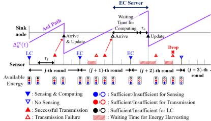
Figure 2: Example path of $\Delta_{n}^{\text{rx}}(t)$ for EH model.

For the data of the $n$-th sensor, the AoI can be defined at both the sensor and the sink node, denoted as $\Delta_{n}^{\text{tx}}(t)$ and $\Delta_{n}^{\text{rx}}(t)$, respectively. The AoI at the sensor, $\Delta_{n}^{\text{tx}}(t)$, becomes $\tau_{\text{t}}$ (i.e., one time slot length) when the sensor obtains new data by sensing. Otherwise, the AoI increases linearly over the time. On the other hand, the AoI at the sink node, $\Delta_{n}^{\text{rx}}(t)$, is defined as the time gap from sensing to the time when the sink node obtains the computed data. Hence, $\Delta_{n}^{\text{tx}}(t)$ and $\Delta_{n}^{\text{rx}}(t)$ are respectively given by

$$\Delta_{n}^{\text{tx}}(t)=t-{t}^{\text{tx}}_{\text{g},n},$$ (7)

$$\Delta_{n}^{\text{rx}}(t)=t-{t}^{\text{rx}}_{\text{g},n},$$ (8)

where ${t}^{\text{tx}}_{\text{g},n}$ is the latest data generation time at the $n$-th sensor, and ${t}^{\text{rx}}_{\text{g},n}$ is the generation time of the lately updated data of the $n$-th sensor at the sink node. Note that $\Delta_{n}^{\text{rx}}(t)$ and $\Delta_{n}^{\text{tx}}(t)$ will be used for defining and analyzing the $\eta$-coverage probability in Section II, III and the RL-based algorithm in Section IV, respectively.

Figure 2 represents an example path of $\Delta_{n}^{\text{rx}}(t)$ over time for $\tau_{\text{r}}=6,\tau_{\text{e}}=1,\tau_{\ell}=2$, and $\delta=2$ for the EH model. At the beginning of the $j$-th round, the $n$-th sensor decides to perform sensing and choose LC. After sensing and computing at the sensor, the sensor transmits the computed data to the sink node, and $\Delta_{n}^{\text{rx}}(t)$ is updated once it is successfully received. At the beginning of the $(j+1)$-th round, the sensor decides to perform sensing and choose EC. Since the sensor does not have sufficient energy for transmission, it waits to get more energy by harvesting. Once the data is successfully received at the sink node, $\Delta_{n}^{\text{rx}}(t)$ can be updated after completing the computation. Here, when the transmission fails $\delta$ (e.g., two in this example) times, the data is dropped as shown in the $(j+2)$-th round.

In sensor networks, the sensed data is generally correlated in time and space [34]. Hence, we can estimate the data at certain point y at time $t$ with the lately generated or updated data of the $n$-th sensor, located at $\textbf{x}_{n}$, at time ${t}^{\text{tx}}_{\text{g},n}$ or ${t}^{\text{rx}}_{\text{g},n}$. Here, the estimator of the data that minimizes the mean square error becomes the conditional expectation, which is given by [34]

$$\hat{H}=\mathbb{E}\left[H(\textbf{y},t)|H(\textbf{x}_{n},{t}^{\iota}_{\text{g},n})\right],\iota\in\{\text{tx, rx}\},$$ (9)

where $H(\textbf{z},t)$ is the data at z and the time $t$.

When the sensed data follows a stationary Gaussian process, the correlation coefficient is represented using the covariance model with the AoI, i.e., $\Delta_{n}^{\iota}(t)=t-{t}^{\iota}_{\text{g},n}$, given by [13]

$$\rho_{\textbf{x}_{n},\textbf{y}}(\Delta_{n}^{\iota}(t))=\exp{(-\beta_{1}d_{\textbf{x}_{n},\textbf{y}}-\beta_{2}\Delta_{n}^{\iota}(t))},\iota\in\{\text{tx, rx}\},$$ (10)

where $d_{\textbf{x}_{n},\textbf{y}}$ is the Euclidean distance between $\textbf{x}_{n}$ and y, $\beta_{1}$ and $\beta_{2}$ are the weights of the spatial error and temporal error, respectively. Since the variance of the estimation error of (9) linearly increases with $1-\{\rho_{\textbf{x}_{n},\textbf{y}}(\Delta_{n}^{\iota}(t))\}^{2}$ [34], the estimation error at y is determined by (10) as [13]

$$\begin{aligned} \epsilon_{\textbf{x}_{n},\textbf{y}}(\Delta_{n}^{\iota}(t))&=1-\{\rho_{\textbf{x}_{n},\textbf{y}}(\Delta_{n}^{\iota}(t))\}^{2}\\ &=1-\exp{(-2\beta_{1}d_{\textbf{x}_{n},\textbf{y}}-2\beta_{2}\Delta_{n}^{\iota}(t))},\iota\in\{\text{tx, rx}\}.\end{aligned}$$ (11)

From (11), we can observe that the estimation error increases as $d_{\textbf{x}_{n},\textbf{y}}$ increases or $\Delta_{n}^{\iota}(t)$ increases. We assume the estimated data of y at $t$ from the sensed data at $\textbf{x}_{n}$ and time ${t}^{\iota}_{\text{g},n}$ becomes invalid when the estimation error, $\epsilon_{\textbf{x}_{n},\textbf{y}}(\Delta_{n}^{\iota}(t))$, is greater than the threshold $\epsilon_{0}$ as

$$\epsilon_{\textbf{x}_{n},\textbf{y}}(\Delta_{n}^{\iota}(t))>\epsilon_{0},\iota\in\{\text{tx, rx}\}.$$ (12)

Then, the sensing coverage of the $n$-th sensor can be defined as the area that the sensed data can be used to estimate the data of the area with less error than $\epsilon_{0}$ [35]. The sensing coverage becomes a circle with radius $r_{\text{c}}(\Delta_{n}^{\iota}(t),\epsilon_{0})$, given by

$$r_{\text{c}}(\Delta_{n}^{\iota}(t),\epsilon_{0})=\frac{-2\beta_{2}\Delta_{n}^{\iota}(t)-\log(1-\epsilon_{0})}{2\beta_{1}},\iota\in\{\text{tx, rx}\},$$ (13)

which can be obtained by substituting (11) into (12) for $\epsilon_{\textbf{x}_{n},\textbf{y}}(\Delta_{n}^{\iota}(t))=\epsilon_{0}$. Since the sink node collects and manages the information of sensors, we focus on the AoI at the sink node, i.e., $\Delta_{n}^{\text{rx}}(t)$, and from (13), we can see that $r_{\text{c}}(\Delta_{n}^{\text{rx}}(t),\epsilon_{0})$ decreases as $\Delta_{n}^{\text{rx}}(t)$ increases.

Next, we define the error-tolerable network coverage ratio from the sensing coverage model. We consider a 2-D discrete grid network $\Phi$. We define an event $c_{\textbf{x}_{n},\textbf{y}}(t)$ that the point at y is in the coverage of the $n$-th sensor at time $t$, given by

$$c_{\textbf{x}_{n},\textbf{y}}(t)=\begin{cases}1,&d_{\textbf{x}_{n},\textbf{y}}\leq r_{\text{c}}(\Delta_{n}^{\text{rx}}(t),\epsilon_{0}),\\ 0,&\mbox{otherwise}.\end{cases}$$ (14)

Since the sensor network consists of multiple sensors, we can regard the point at y is in the network coverage if it is covered by at least one sensor. Here, the sink node uses the data which has the minimum estimation error among the sensors, i.e., $\displaystyle\min_{n\in\mathcal{N}}\epsilon_{\textbf{x}_{n},\textbf{y}}(\Delta_{n}^{\text{rx}}(t))$. Then, whether the point at y is covered or not in the network is indicated as $C_{\textbf{y}}\in\{0,1\}$, given by

$$C_{\textbf{y}}(t)=1-\prod_{n\in\mathcal{N}}(1-c_{\textbf{x}_{n},\textbf{y}}(t)).$$ (15)

From (15), at time $t$, we can define the network coverage ratio $\phi_{\text{cov}}(t)$ as the ratio of the area, covered by at least one sensor, to the whole network area $|\Phi|$ as

$$\phi_{\text{cov}}(t)=\frac{\sum_{\textbf{y}\in\Phi}C_{\textbf{y}}(t)}{|\Phi|}.$$ (16)

Finally, we define the $\eta$-coverage probability $\mathcal{P}_{\text{c}}(\eta)$ as the probability that $\phi_{\text{cov}}(t)$ is larger than a target coverage ratio $\eta$, which is given by [35]

$$\mathcal{P}_{\text{c}}(\eta)=\mathbb{P}[\phi_{\text{cov}}(t)\geq\eta].$$ (17)

Note that $\mathcal{P}_{\text{c}}(\eta)$ can also show the portion of the network area where the sink node has the data with smaller error than $\epsilon_{0}$.

II-E Two SCD Approaches

To enhance the $\eta$-coverage probability, we can design the SCD algorithm in two approaches: 1) the probability-based SCD and 2) the RL-based SCD. For the probability-based SCD, the optimal probabilities for sensing and EC, which maximize the $\eta$-coverage probability in average sense, are used without requiring the real-time information from other sensors or EC server. However, in this algorithm, the sensors cannot utilize network status such as the AoI and battery level, which may lead to a low performance. On the other hand, in the RL-based SCD, each sensor makes the decision based on the current network status to improve the $\eta$-coverage probability through the training process. Specifically, the real-time information of the network status such as the AoI and the battery level are needed, but it generally achieves the higher performance than the probability-based SCD algorithm as it makes decisions based on the current status information. In the following sections, we provide the probability-based SCD algorithm (Section III) and the RL-based SCD algorithm (Section IV).

III Probability-based SCD Algorithm

In this section, we propose the probability-based SCD algorithm, which determines to sense with the probability $p_{\text{s}}$ and determines to compute at the EC server with the probability $p_{\text{e}}$ at each round. To maximize the $\eta$-coverage probability, we optimize $p_{\text{s}}$ and $p_{\text{e}}$ in the probability-based SCD algorithm. For that, in this section, we first derive the $\eta$-coverage probability for the single pre-charged sensor case, and provide the optimal $p_{\text{s}}$ and $p_{\text{e}}$. We then discuss how to obtain the optimal $p_{\text{s}}$ and $p_{\text{e}}$ for the multiple EH sensor case.

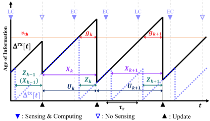
Figure 3: Example of the AoI path of the single pre-charged sensor case, $\Delta^{\text{tx}}(t)$ and $\Delta^{\text{rx}}(t)$, from the $(k-1)$-th to the $(k+1)$-th successful update.

III-A Single Pre-Charged Sensor Case

III-A1 $\eta$-Coverage Probability Analysis

We first analyze the $\eta$-coverage probability in the single pre-charged sensor case. Here, we consider a 2-D network $\Phi_{\text{sg}}$ with a sink node and a sensor, and omit index $n$ for simplicity. In this case, $C_{\textbf{y}}(t)$ in (15) becomes $c_{\textbf{x},\textbf{y}}(t)$, and in (16), we have $\sum_{\textbf{y}\in\Phi_{\text{sg}}}C_{\textbf{y}}(t)=\sum_{\textbf{y}\in\Phi_{\text{sg}}}c_{\textbf{x},\textbf{y}}(t)$, which indicates the sensing coverage of the sensor. The radius of the sensing coverage is $r_{\text{c}}(\Delta^{\text{rx}}(t),\epsilon_{0})$, so the sensing coverage area can be presented as $\pi r_{\text{c}}^{2}(\Delta^{\text{rx}}(t),\epsilon_{0})$. When the sensing coverage is completely included in $\Phi_{\text{sg}}$, $\phi_{\text{cov}}(t)$ can be given by

$$\phi_{\text{cov}}(t)=\frac{\pi r_{\text{c}}^{2}(\Delta^{\text{rx}}(t),\epsilon_{0})}{|\Phi_{\text{sg}}|}=\frac{\pi\{-2\beta_{2}\Delta^{\text{rx}}(t)-\log(1-\epsilon_{0})\}^{2}}{4\beta_{1}^{2}|\Phi_{\text{sg}}|},$$ (18)

where $|\Phi_{\text{sg}}|$ is the considered network area in the single sensor case. From (17) and (18), $\mathcal{P}_{\text{c}}(\eta)$ is given by

$$\begin{aligned} \mathcal{P}_{\text{c}}(\eta)&=\mathbb{P}\left[\frac{\pi\{-2\beta_{2}\Delta^{\text{rx}}(t)-\log(1-\epsilon_{0})\}^{2}}{4\beta_{1}^{2}|\Phi_{\text{sg}}|}\geq\eta\right]\\ &=1-\mathbb{P}\left[\Delta^{\text{rx}}(t)>v_{\text{th}}\right],\end{aligned}$$ (19)

where the target AoI is $v_{\text{th}}=-\frac{\beta_{1}}{\beta_{2}}\sqrt{\frac{\eta|\Phi_{\text{sg}}|}{\pi}}-\frac{\log(1-\epsilon_{0})}{2\beta_{2}}$. From (19), we can see that in the single pre-charged sensor case, the $\eta$-coverage probability can be represented as the AoI violation probability $\mathbb{P}\left[\Delta^{\text{rx}}(t)>v_{\text{th}}\right]$, which is the probability that the AoI, $\Delta^{\text{rx}}(t)$, violates the target AoI $v_{\text{th}}$.

For the analysis of the $\eta$-coverage probability, we first define some time intervals in the AoI path as follows. An example of the AoI path of the single pre-charged sensor case, $\Delta^{\text{tx}}(t)$ and $\Delta^{\text{rx}}(t)$, from the $(k-1)$-th to the $(k+1)$-th successful update are presented in Fig. 3. For the $k$-th successful update, we denote the time interval from the sensing instance to the successful update as $Z_{k}$, the time interval from the beginning of the first round after the $(k-1)$-th successful update to the $k$-th successful update time as $X_{k}$, the inter update time as $U_{k}$, and the violation time for $k$-th successful update as $g_{k}$. We use $m_{k}\in\{\text{e},\ell\}$ to indicate whether the information of the $k$-th successful update is computed by the EC ($m_{k}=\text{e}$) or LC ($m_{k}=\ell$).

Next, we analytically obtain the $\eta$-coverage probability in (19) for the single pre-charged sensor case. we first assume sensing, computing, and transmission caused by the current round are completed before starting the next round, i.e., $1+\delta+\tau_{k}\leq\tau_{\text{r}},\tau_{k}\in\{\tau_{\text{e}},\tau_{\ell}\}$. Note that for the single sensor case, we assume that the waiting time at the EC server is negligible as it only handles the information from one sensor.

The AoI violation probability is given by [36]

$$\mathbb{P}\left[\Delta^{\text{rx}}(t)>v_{\text{th}}\right]=\frac{\mathbb{E}[g_{k}]}{\mathbb{E}[U_{k}]},$$ (20)

where $\mathbb{E}[U_{k}]$ and $\mathbb{E}[g_{k}]$ are the expected inter-update and violation time, respectively. Here, $U_{k}$ and $g_{k}$ are presented as

$$U_{k}=\tau_{\text{r}}-Z_{k-1}+X_{k},$$ (21)

$$g_{k}=\begin{cases}\tau_{\text{r}}+X_{k}-Z_{k-1},&\mathrm{if}\quad v_{\text{th}}<Z_{k-1},\\ \tau_{\text{r}}+X_{k}-(\lfloor v_{\text{th}}\rfloor+1),&\mathrm{if}\quad Z_{k-1}\leq v_{\text{th}}<\tau_{\text{r}}+X_{k},\\ 0,&\mathrm{if}\quad\tau_{\text{r}}+X_{k}\leq v_{\text{th}},\end{cases}$$ (22)

where $\lfloor x\rfloor$ is a floor function that gives the greatest integer less than or equal to $x$. In the following lemma, we obtain $\mathbb{E}[U_{k}]$ for given $p_{\text{s}}$ and $p_{\text{e}}$.

Lemma 1 (Expected Inter-Update Time)

The expected inter-update time $\mathbb{E}[U_{k}]$ in (20) is obtained as

$$\mathbb{E}[U_{k}]=\frac{\tau_{\text{r}}}{p_{\delta}},$$ (23)

where $p_{\delta}$ is given by

$$\begin{aligned} p_{\delta}&=p_{\text{s}}[p_{\text{e}}\{1-(p_{\textbf{o},{\text{e}}})^{{\delta}}\}+(1-p_{\text{e}})\{1-(p_{\textbf{o},{\ell}})^{{\delta}}\}].\end{aligned}$$ (24)

Proof:

See Appendix -A. ∎

In the following lemma, we also obtain $\mathbb{E}[g_{k}]$ for given $p_{\text{s}}$ and $p_{\text{e}}$.

Lemma 2 (Expected Violation Time)

$\mathbb{E}[g_{k}]$ in (20) is obtained as

$$\begin{aligned} \mathbb{E}[g_{k}]=\sum_{m_{k-1}\in\{\text{e},\ell\}}\sum_{m_{k}\in\{\text{e},\ell\}}p_{\text{u}}(m_{k-1})p_{\text{u}}(m_{k})G(m_{k-1},m_{k}),\end{aligned}$$ (25)

where $p_{\text{u}}(m_{k})$ is the probability that EC ($m_{k}=\text{e}$) or LC ($m_{k}=\ell$) is chosen, conditioned on the successful update, given by

$$p_{\text{u}}(m_{k})=\begin{cases}\frac{p_{\text{e}}\{1-(p_{\textbf{o},{\text{e}}})^{{\delta}}\}}{p_{\text{e}}\{1-(p_{\textbf{o},{\text{e}}})^{{\delta}}\}+(1-p_{\text{e}})\{1-(p_{\textbf{o},{\ell}})^{{\delta}}\}},&\mathrm{if}\quad m_{k}=\text{e},\\ \frac{(1-p_{\text{e}})\{1-(p_{\textbf{o},{\ell}})^{{\delta}}\}}{p_{\text{e}}\{1-(p_{\textbf{o},{\text{e}}})^{{\delta}}\}+(1-p_{\text{e}})\{1-(p_{\textbf{o},{\ell}})^{{\delta}}\}},&\mathrm{if}\quad m_{k}=\ell.\end{cases}$$ (26)

Here, $G(m_{k-1},m_{k})$ is presented in (32) according to the range of $v_{\text{th}}$, where

$$\begin{aligned} v_{1,k}&=2+\tau_{k-1},\\ v_{2,k}&=1+\delta+\tau_{k-1},\\ v_{3,k}(y)&=y\tau_{\text{r}}+2+\tau_{k},\\ v_{4,k}(y)&=y\tau_{\text{r}}+1+\delta+\tau_{k},\\ \end{aligned}$$ (27)

for $y=1,2,\cdots$. In (32), $\varrho_{c,k},f_{\delta,k},h_{\delta,k}({y})$ and $\kappa_{k}(y)$ are respectively defined as

$$\varrho_{c,k} =1-(p_{\textbf{o},{k}})^{{c}},c\in\{1,2,\cdots,\delta\},$$ (28)

$$f_{\delta,k} =\frac{1}{\varrho_{1,k}}-\frac{\delta p_{\textbf{o},{k}}^{\delta}\varrho_{1,k}}{\varrho_{\delta,k}},$$ (29)

$$h_{\delta,k}({y}) =1+\delta+\tau_{k}+\tau_{\text{r}}(y-1),$$ (30)

$$\kappa_{k}(y) =\lfloor v_{\text{th}}\rfloor-\tau_{k}-\tau_{\text{r}}y-1.$$ (31)

$G(m_{k-1},m_{k})=$

$$\begin{aligned} \begin{cases}\frac{\tau_{\text{r}}}{p_{\delta}}+\tau_{k}-\tau_{k-1}+f_{\delta,k}-f_{\delta,k-1},&v_{\text{th}}<v_{1,k},\\ \frac{\tau_{\text{r}}}{p_{\delta}}+\tau_{k}-\tau_{k-1}+f_{\delta,k}-\frac{\lfloor v_{\text{th}}\rfloor-\tau_{k-1}-p_{\textbf{o},{k-1}}^{\lfloor v_{\text{th}}\rfloor-1-\tau_{k-1}}-\delta p_{\textbf{o},{k-1}}^{\delta}}{\varrho_{\delta,k-1}}-\frac{p_{\textbf{o},{k-1}}^{\lfloor v_{\text{th}}\rfloor-1-\tau_{k-1}}-p_{\textbf{o},{k-1}}^{\delta}}{\varrho_{\delta,k-1}\varrho_{1,k-1}},&v_{1,k}\leq v_{\text{th}}<v_{2,k},\\ \frac{\tau_{\text{r}}}{p_{\delta}}+\tau_{k}+f_{\delta,k}-\lfloor v_{\text{th}}\rfloor,&v_{2,k}\leq v_{\text{th}}<v_{3,k}(y=1),\\ (1-p_{\delta})^{y-1}\left[(1-p_{\delta})\left\{h_{\delta,k}({y})+\frac{\tau_{\text{r}}}{p_{\delta}}-\frac{\delta}{\varrho_{\delta,k}}+\frac{1}{\varrho_{1,k}}\right\}+(1-\tau_{\text{r}}+\lfloor v_{\text{th}}\rfloor)\left\{\frac{p_{\delta}\varrho_{\kappa_{k}(y),k}}{\varrho_{\delta,k}}-1\right\}\right.\\ \left.\qquad\qquad\qquad+\frac{p_{\delta}}{\varrho_{\delta,k}}\left\{\varrho_{1,k}^{\kappa_{k}(y)}(\lfloor v_{\text{th}}\rfloor-\tau_{\text{r}})-\varrho_{1,k}^{\delta}h_{\delta,k}({y})+\frac{\varrho_{1,k}^{\kappa_{k}(y)}-\varrho_{1,k}^{\delta}}{p_{\textbf{o},{k}}}\right\}\right],&v_{3,k}(y)\leq v_{\text{th}}<v_{4,k}(y),\\ (1-p_{\delta})^{y}\left\{-\kappa_{k}(y)-1+\frac{\tau_{\text{r}}}{p_{\delta}}+\frac{1}{\varrho_{1,k}}+\delta\left(1-\frac{1}{\varrho_{\delta,k}}\right)\right\},&v_{4,k}(y)\leq v_{\text{th}}<v_{3,k}(y+1).\\ \end{cases}\end{aligned}$$ (32)

 

Proof:

See Appendix -B. ∎

From Lemma 1 and Lemma 2, the AoI violation probability $\mathbb{P}\left[\Delta^{\text{rx}}(t)>v_{\text{th}}\right]$ is then derived by dividing $\mathbb{E}[g_{k}]$ into $\mathbb{E}[U_{k}]$ as (20). Finally, by using (20) in (19), we can obtain the $\eta$-coverage probability for the single pre-charged sensor case for given $p_{\text{s}}$ and $p_{\text{e}}$, obtained as

$$\begin{aligned} &\mathcal{P}_{\text{c}}^{\eta}(p_{\text{s}},p_{\text{e}})\\ &=1-\frac{p_{\delta}}{\tau_{\text{r}}}\sum_{m_{k-1}\in\{\text{e},\ell\}}\sum_{m_{k}\in\{\text{e},\ell\}}p_{\text{u}}(m_{k-1})p_{\text{u}}(m_{k})G(m_{k-1},m_{k}).\end{aligned}$$ (33)

Here, we change the notation $\mathcal{P}_{\text{c}}(\eta)$ to $\mathcal{P}_{\text{c}}^{\eta}(p_{\text{s}},p_{\text{e}})$ to use it for optimizing $p_{\text{s}}$ and $p_{\text{e}}$ in the following section.

III-A2 Optimal Probability of Sensing and Computing

We obtain the optimal $p_{\text{s}}$ and $p_{\text{e}}$ that maximize the $\eta$-coverage probability. For that, we first obtain the average energy consumption per the time duration of a round $\tau_{\text{r}}$, denoted as $\bar{E}_{t}$. The average energy consumption over $\tau_{\text{r}}$ when the sensor chooses EC, $\bar{E}_{\text{e}}$, is given by

$$\begin{aligned} \bar{E}_{\text{e}}=E_{\text{S}}+E_{\text{T}}\bar{N}_{\text{e}}(p_{\textbf{o},{\text{e}}}),\end{aligned}$$ (34)

where $\bar{N}_{m_{k}}(p_{\textbf{o},{k}})$ is the average number of transmissions, given by

$$\bar{N}_{m_{k}}(p_{\textbf{o},{k}})=\sum_{c=1}^{\delta}cp_{\textbf{o},{k}}^{c-1}(1-p_{\textbf{o},{k}})+\delta p_{\textbf{o},{k}}^{\delta}=\frac{\varrho_{\delta,k}}{\varrho_{1,k}}.$$ (35)

Similarly, the average energy consumption over $\tau_{\text{r}}$ when the sensor chooses LC, $\bar{E}_{\ell}$, is given by

$$\begin{aligned} \bar{E}_{\ell}&=E_{\text{S}}+E_{\text{C}}+E_{\text{T}}\bar{N}_{\ell}(p_{\textbf{o},{\ell}}).\end{aligned}$$ (36)

For given $p_{\text{s}}$ and $p_{\text{e}}$, $\bar{E}_{t}$ is then obtained as

$$\begin{aligned} \bar{E}_{t}=p_{\text{s}}p_{\text{e}}\bar{E}_{\text{e}}+p_{\text{s}}(1-p_{\text{e}})\bar{E}_{\ell}.\end{aligned}$$ (37)

Note that the consumed energy over $N_{\text{r}}$ rounds needs to be less than or equal to $B_{\text{th}}$ in the pre-charged battery model, i.e., $N_{\text{r}}\bar{E}_{t}\leq B_{\text{th}}$, as described in Section II-C.

We now formulate the $\eta$-coverage probability maximization problem for the single pre-charged sensor case.

Problem 1 ($\eta$-Coverage Probability Maximization in Single Pre-Charged Sensor Case):

$$\max_{p_{\text{s}},p_{\text{e}}}\qquad \mathcal{P}_{\text{c}}^{\eta}(p_{\text{s}},p_{\text{e}})$$ (38)

s.t. $${N_{\text{r}}\bar{E}_{t}\leq B_{\text{th}},}$$ (39)

$$0\leq p_{\text{s}}\leq 1,$$ (40)

$$0\leq p_{\text{e}}\leq 1.$$ (41)

To solve Problem 1, we first discuss the effect of $p_{\text{s}}$ on $\mathcal{P}_{\text{c}}^{\eta}(p_{\text{s}},p_{\text{e}})$ in the following remark.

Remark 1

For given $p_{\text{e}}$, $\mathcal{P}_{\text{c}}^{\eta}(p_{\text{s}},p_{\text{e}})$ is a monotonically increasing function of $p_{\text{s}}$. For example, for $v_{1,k}\leq v_{\text{th}}<v_{2,k}$ for both $m_{k-1}=\text{e}$ and $m_{k-1}=\ell$, i.e., $2+\tau_{\text{e}}\leq 2+\tau_{\ell}\leq v_{\text{th}}<1+\delta+\tau_{\text{e}}\leq 1+\delta+\tau_{\ell}$, the first derivative of $\mathcal{P}_{\text{c}}^{\eta}(p_{\text{s}},p_{\text{e}})$ with respect to $p_{\text{s}}$ is given by

$$\begin{aligned} \frac{\partial\mathcal{P}_{\text{c}}^{\eta}(p_{\text{s}},p_{\text{e}})}{\partial p_{\text{s}}}=\frac{1}{\tau_{\text{r}}}&\Bigg{[}\lfloor v_{\text{th}}\rfloor-\{p_{\text{e}}\tau_{\text{e}}+(1-p_{\text{e}})\tau_{\ell}\}\\ &-\left\{p_{\text{e}}\frac{\varrho_{\lfloor v_{\text{th}}\rfloor-\tau_{\text{e}},\text{e}}}{\varrho_{1,\text{e}}}+(1-p_{\text{e}})\frac{\varrho_{\lfloor v_{\text{th}}\rfloor-\tau_{\ell},\ell}}{\varrho_{1,\ell}}\right\}\Bigg{]}.\end{aligned}$$ (42)

Here, from (28), $\varrho_{\lfloor v_{\text{th}}\rfloor-\tau_{\text{e}},\text{e}}/\varrho_{1,\text{e}}$ and $\varrho_{\lfloor v_{\text{th}}\rfloor-\tau_{\ell},\ell}/\varrho_{1,\ell}$ in (42) are expressed as

$$\begin{aligned} \frac{\varrho_{\lfloor v_{\text{th}}\rfloor-\tau_{k},k}}{\varrho_{1,k}}&=\frac{1-(p_{\textbf{o},{k}})^{{\lfloor v_{\text{th}}\rfloor-\tau_{k}}}}{1-p_{\textbf{o},{k}}}\\ &=\sum_{c=0}^{\lfloor v_{\text{th}}\rfloor-\tau_{k}-1}(p_{\textbf{o},{k}})^{c}<\lfloor v_{\text{th}}\rfloor-\tau_{k},m_{k}\in\{\text{e},\ell\},\end{aligned}$$ (43)

where the inequality in (43) holds since the outage probability is less than 1, i.e., $p_{\textbf{o},{k}}<1$. Then, from (43), (42) can be obtained as

$$\begin{aligned} \frac{\partial\mathcal{P}_{\text{c}}^{\eta}(p_{\text{s}},p_{\text{e}})}{\partial p_{\text{s}}}&>\frac{1}{\tau_{\text{r}}}\Big{[}\lfloor v_{\text{th}}\rfloor-\{p_{\text{e}}\tau_{\text{e}}+(1-p_{\text{e}})\tau_{\ell}\}\\ &-\left\{p_{\text{e}}(\lfloor v_{\text{th}}\rfloor-\tau_{\text{e}})+(1-p_{\text{e}})(\lfloor v_{\text{th}}\rfloor-\tau_{\ell})\right\}\Big{]}=0.\end{aligned}$$ (44)

Thus, $\mathcal{P}_{\text{c}}^{\eta}(p_{\text{s}},p_{\text{e}})$ is a monotonically increasing function of $p_{\text{s}}$.

Let $p_{\text{s}}^{\star}(p_{\text{e}})$ denote an optimal sensing probability for given $p_{\text{e}}$. We equivalently convert the constraint in (37) to

$$p_{\text{s}}\leq\frac{B_{\text{th}}}{N_{\text{r}}\{\bar{E}_{\text{e}}p_{\text{e}}+\bar{E}_{\ell}(1-p_{\text{e}})\}}.$$ (45)

Therefore, from (45) and Remark 1, $p_{\text{s}}^{\star}(p_{\text{e}})$, is obtained as

$$p_{\text{s}}^{\star}(p_{\text{e}})=\min{\left[\frac{B_{\text{th}}}{N_{\text{r}}\{\bar{E}_{\text{e}}p_{\text{e}}+\bar{E}_{\ell}(1-p_{\text{e}})\}},1\right]}.$$ (46)

Unlike $p_{\text{s}}$, it is not guaranteed that $\mathcal{P}_{\text{c}}^{\eta}(p_{\text{s}},p_{\text{e}})$ monotonically increases or decreases with $p_{\text{e}}$. Specifically, the trend of $\mathcal{P}_{\text{c}}^{\eta}(p_{\text{s}},p_{\text{e}})$ with $p_{\text{e}}$ depends on parameters such as the outage probability, the computing energy, and the computing time. Therefore, we use an exhaustive search to obtain $(p_{\text{s}}^{*},p_{\text{e}}^{*})$, i.e., $p_{\text{e}}^{*}=\mathop{\mathrm{argmax}}_{p_{\text{e}}}\mathcal{P}^{\eta}_{\text{c}}\Big{(}p_{\text{s}}^{\star}(p_{\text{e}}),p_{\text{e}}\Big{)}$ and $p_{\text{s}}^{*}=p_{\text{s}}^{\star}(p_{\text{e}}^{*})$.

III-B Multiple EH Sensor Case

In the multiple EH sensor case, it is difficult to clearly analyze the effect of $p_{\text{s}}$ and $p_{\text{e}}$ on $\mathcal{P}_{\text{c}}^{\eta}(p_{\text{s}},p_{\text{e}})$ by deriving the AoI violation probability due to the overlapped coverage of the sensors. Furthermore, it is hard to formulate the optimization problem for the probability-based SCD algorithm in EH case since the energy level of sensor dynamically changes and the sensor cannot perform sensing even it is decided to sense when the battery is insufficient. Thus, in the multiple EH sensor case, we need to obtain the optimal solution $(p_{\text{s}}^{*},p_{\text{e}}^{*})$ using the exhaustive search by evaluating the $\eta$-coverage probability using simulation.

In the probability-based SCD algorithm, even though $(p_{\text{s}}^{*},p_{\text{e}}^{*})$ can be obtainable, it is difficult to obtain the high $\eta$-coverage probability since this algorithm cannot consider the real-time dynamics. For instance, when the battery level is low, decreasing the frequency of sensing may increase the $\eta$-coverage probability by reducing the energy consumption. However, the sensor in the probability-based SCD algorithm cannot make dynamic decision. Therefore, in the following section, we develop an algorithm where each sensor can make real-time decision in the dynamic and complex environment to enhance the $\eta$-coverage probability in the EC-enabled wireless sensor networks.

IV RL-based SCD Algorithm

In this section, we propose the RL-based SCD algorithm to maximize the $\eta$-coverage probability. Firstly, we formulate a partially observable Markov decision process (POMDP) problem for both the single pre-charged and the multiple EH sensor cases, and then develop an RL algorithm and a network architecture to solve the POMDP problems.

IV-A POMDP Formulation

In the RL-based SCD algorithm, sensors are trained to make the decision in the way of maximizing the $\eta$-coverage probability. In this algorithm, we consider an episodic environment with the episode length $T_{\text{ep}}$, where each episode consists of $N_{\text{r}}$ rounds, i.e., $T_{\text{ep}}=N_{\text{r}}\tau_{\text{r}}$.

Next, we consider an $N_{\text{s}}$-agent POMDP, where the $n$-th agent makes an action $a_{n}[j]$ based on the observation $o_{n}[j]$ and obtains a reward $r_{n}[j]$ at the $j$-th round. Each agent aims to maximize a return $R_{n}=\sum_{j=1}^{N_{\text{r}}}\gamma^{j-1}r_{n}[j]$, where $\gamma\in[0,1]$ is a discount factor. In the presented EC-enabled wireless sensor networks, the $\eta$-coverage probability maximization problem can be formulated as the POMDP, where each sensor acts as an agent. The observation, action, and reward of each sensor are given as follows.

• Observation: Each sensor has its observation range $d_{\text{obs}}$. Then, the observed sensor set at the $n$-th sensor, $\tilde{\mathcal{N}}_{n}$, is given by

  $$\tilde{\mathcal{N}}_{n}=\{m|d_{\textbf{x}_{n},\textbf{x}_{m}}\leq d_{\text{obs}},m\in\mathcal{N}\},$$ (47)

  where $d_{\textbf{x}_{n},\textbf{x}_{m}}$ is the distance between the $n$-th and $m$-th sensors. When the $j$-th round begins, i.e., $\tilde{t}_{j}$, the observation of the $n$-th sensor contains the information of sensors in $\tilde{\mathcal{N}}_{n}$, given by

  $$o_{n}[j]=(\{B_{m}(\tilde{t}_{j}),\Delta_{m}^{\text{rx}}(\tilde{t}_{j}),\Delta_{m}^{\text{tx}}(\tilde{t}_{j})|m\in\tilde{\mathcal{N}}_{n}\},s_{n}^{\text{w}}(\tilde{t}_{j})).$$ (48)

  As shown in (48), the observation contains the information about the battery level, the AoI at the sensor and the sink node side of sensors in $\tilde{\mathcal{N}}_{n}$, and the local information on the waiting time at the EC server, $s_{n}^{\text{w}}(\tilde{t}_{j})$.

• Action: Each sensor independently makes SCD as an action at the start of each round. The action for the $n$-th sensor at the $j$-th round is denoted as $a_{n}[j]\in\{\text{EC, LC, IDLE}\}$, where EC denotes the sensing with EC, LC denotes the sensing with LC, and IDLE denotes no sensing and computing. Here, the sensor can choose EC or LC only when the battery level of the sensor is sufficient for performing sensing, i.e., $B_{n}(\tilde{t}_{j})\geq E_{\text{S}}$.

• Reward: The objective of the problem is to maximize the $\eta$-coverage probability. For this, in the episodic environment, we set the reward of the $n$-th sensor as

  $$r_{n}[j]=\sum_{i=0}^{\tau_{\text{r}}-1}\left(\mathbbm{1}[\phi_{\text{cov}}(t^{\prime})\geq\eta]-\nu\mathbbm{1}[\phi_{\text{cov}}(t^{\prime})<\eta]\right),$$ (49)

  where $t^{\prime}=\{(j-1)\tau_{\text{r}}+i\}\tau_{\text{t}}$ and $\nu$ is the penalty factor. Here, we set all sensors to get the shared reward, i.e., $r_{n}[j]=r[j],\forall n\in\mathcal{N}$.

Figure 4: Proposed RL-based SCD algorithm. For readability, the neural networks for only two sensors are shown in the figure.

IV-B Proposed Network Architecture

We develop the RL-based SCD algorithm by implementing the centralized training with decentralized execution (CTDE) framework, as shown in Fig. 4. The proposed algorithm contains the actor and critic networks for each sensor. Moreover, the target actor and the critic networks are separated from the original networks to stabilize the training. Specifically, each sensor makes the decision using its actor network, which can reduce the action dimension and communication burden compared to the centralized execution framework. On the other hand, the critic network estimates the action-value function and aims to minimize the temporal-difference error. In addition, the sink node collects the observation, the action, and the reward from the sensors to centrally train the actor and critic network parameters.

The pseudo-code of the proposed algorithm is given in Algorithm. The objective of the proposed algorithm is to train the actor network and critic network of the sensors, parameterized by $\theta_{n}$ and $\omega_{n}$, respectively. Moreover, the target actor and the critic networks are separated from the original networks to stabilize the learning, parameterized by $\theta^{\prime}_{n}$ and $\omega^{\prime}_{n}$, respectively. We train the neural networks over the $T_{\text{train}}$ episodes, and at the beginning of each episode, observations, actions, and rewards of the sensors are initialized (Line 2). Here, the bold symbols $\mathbf{o}$ and $\mathbf{a}$ are the observations and actions of the all sensors in the current round, i.e., $\mathbf{o}=\{o_{1},\cdots,o_{N_{\text{s}}}\}$ and $\mathbf{a}=\{a_{1},\cdots,a_{N_{\text{s}}}\}$, respectively.

Algorithm 1 Proposed RL-based SCD algorithm.

1:Output: trained network parameters $\omega_{n},\theta_{n},n\in\mathcal{N}$

2:for episode $=1:T_{\text{train}}$ do

3:     Initialize observation $\mathbf{o}$, action $\mathbf{a}$, reward $r$

4:     for round $j=1:N_{\text{r}}$ do

5:         for $n=1:N_{\text{s}}$ do

6:              Select action $a_{n}=G_{\text{gumbel}}(\mu_{\theta_{n}}(o_{n}))$          

7:         for $t=\tilde{t}_{j}:\tau_{\text{t}}:\tilde{t}_{j+1}$ do

8:              Update the network status and calculate $\phi_{\text{cov}}(t)$          

9:         Get shared reward $r$, new observation $\mathbf{o}^{\prime}$

10:         Store $(\mathbf{o,a},r,\mathbf{o}^{\prime})$ in replay buffer      

11:     for $n=1:N_{\text{s}}$ do

12:         Sample a mini-batch of trajectories $(\mathbf{o,a},r,\mathbf{o}^{\prime})$

13:         Update critic parameter $\omega_{n}$ using (50)

14:         Update actor parameter $\theta_{n}$ using (51)

15:         $\omega_{n}^{\prime}\leftarrow\chi\omega_{n}+(1-\chi)\omega_{n}^{\prime}$

16:         $\theta_{n}^{\prime}\leftarrow\chi\theta_{n}+(1-\chi)\theta_{n}^{\prime}$      

At the beginning of each round, each sensor selects and executes the action based on its observation (Line 5). To implement the proposed CTDE-based algorithm, we adopt the multi-agent deep deterministic policy gradient (MADDPG) algorithm [37]. In this algorithm, a deterministic policy, $\mu_{\theta_{n}}$, is used to determine the action from the observation. Here, $G_{\text{gumbel}}(\cdot)$ is Gumbel-Softmax estimator [38], which is used to support a discrete action space. Next, the network status is updated and the network coverage ratio $\phi_{\text{cov}}(t)$ is calculated (Line 7). At the end of each round, sensors obtain the shared reward $r$; the observations of all sensors at the subsequent round $\mathbf{o}^{\prime}$ are updated (Line 8); and the experience $(\mathbf{o,a},r,\mathbf{o}^{\prime})$ is stored in the replay buffer (Line 9).

At the end of each episode, the mini-batch is sampled from the replay buffer, and $\omega_{n},\theta_{n},n\in\mathcal{N}$ are centrally trained at the sink node (Lines 11-13). In order to train $\omega_{n}$, the loss for the critic network, $L(\omega_{n})$, is given by

$$L(\omega_{n})=\mathbb{E}\left[(Q_{\omega_{n}}(\mathbf{o},\mathbf{a})-r-\gamma Q_{\omega_{n}^{\prime}}(\mathbf{o}^{\prime},\mathbf{a}^{\prime}))^{2}\right],$$ (50)

where $Q_{\omega_{n}}(\mathbf{o},\mathbf{a})$ denotes the action-value function, $\omega^{\prime}_{n}$ is the target critic network parameters, and $\mathbf{a}^{\prime}$ is the actions of all sensors at the subsequent round, respectively. Next, the direction of the gradient of the expected return $J(\mu_{\theta_{n}})$, $\nabla_{\theta_{n}}J(\mu_{\theta_{n}})$, is written as

$$\nabla_{\theta_{n}}J(\mu_{\theta_{n}})=\mathbb{E}[\nabla_{\theta_{n}}\mu_{\theta_{n}}(a_{n}|o_{n})\nabla_{a_{n}}Q_{\omega_{n}}(\mathbf{o},\mathbf{a})|_{a_{n}=\mu_{\theta_{n}^{\prime}}(o_{n})}],$$ (51)

where $\theta^{\prime}_{n}$ is the target actor network parameters. Finally, $\theta_{n}^{\prime}$ and $\omega_{n}^{\prime}$ are updated by adopting the soft-update with parameter $\chi$ (Lines 14-15). Note that the proposed RL-based SCD algorithm also can be applied to both the single pre-charged sensor and the multiple EH sensor cases.

Unlike tabular RL environments, the proposed RL-based SCD algorithm, which is the multi-agent deep RL algorithm, generally cannot guarantee the global optimality [39] nor show the performance gain theoretically. This is because the $\eta$-coverage probability is affected by sequential decisions of multiple sensors as well as the excessively many factors such as harvesting energy and channel state information during the episode. However, this algorithm is trained to converge to a local optimum for enhancing the $\eta$-coverage probability. In addition, we leverage the CTDE framework to enhance coordination among the sensors which can improve the performance. Moreover, we further utilize the information of the neighboring sensors by adopting the observation range.

IV-C Complexity Analysis

In this subsection, we provide the complexity analysis about the proposed RL-based SCD algorithm. Here, we focus on the complexity at the sensor, which has limited computational capability and battery, because the training is processed in centralized sink node, which generally has much higher computation capability and sufficient energy. Since the actor network is used to decide the action, the computational complexity for the sensor $n$ is affected by the size of observation, action, and the number of hidden layers and nodes [40, 41]. Hence, the complexity for execution at each round can be expressed as

$${\mathcal{O}\Big{(}|o_{n}|H_{1}+H_{1}H_{2}+\cdots+H_{L_{A}-1}H_{L_{A}}+H_{L_{A}}|a_{n}|\Big{)},}$$ (52)

where $|\cdot|$ is the cardinality of the set, $|a_{n}|=3$ because $a_{n}\in\{\text{EC, LC, IDLE}\}$, $H_{l}$ is the number of hidden nodes of the $l$-th layer, and $L_{A}$ is the number of hidden layers of the actor network. From (48), $|o_{n}|$ depends on the number of the neighboring sensors within the observation range $d_{\text{obs}}$. Hence, the range of $|o_{n}|$ can be determined as

$${4\leq|o_{n}|\leq 3N_{\text{s}}+1,}$$ (53)

which has the minimum value four when there is no neighboring sensor within the observation range, and has the maximum value when the sensor uses the information of all $N_{\text{s}}$ sensors.

V Simulation Results

In this section, we evaluate the performance of proposed probability-based and RL-based SCD algorithms.

TABLE I: Parameter Table

Description	Value	Description	Value
$\tau_{\text{t}}$	$10$ ms	$W$	$10$ MHz
$\tau_{\text{e}}$	$1$	$\tau_{\ell}$	$2$
$\sigma^{2}$	$-100$ dBm	$\lambda$	$10^{-4}$ nodes/$\text{m}^{2}$
$P_{\text{tx}}$	$15$ dBm	$\alpha$	$4$
$\epsilon_{0}$	$0.6$	$\tau_{\text{r}}$	$8$
$L_{\text{e}}$	$6$ Kbit	$L_{\ell}$	$500$ bit
$\beta_{1}$	$0.0045$	$\beta_{2}$	$1.35$
$T_{\text{ep}}$	$20$	$d_{\text{obs}}$	$100$ m
$\gamma$	$0.95$	$T_{\text{train}}$	$20,000$
$\chi$	$0.005$	$\nu$	$1$

We set $N_{\text{r}}=20$, $\delta=3$, $E_{\mathrm{S}}=10$ (mJ), $E_{\text{T}}=13.55$ (mJ) [42], $p_{\text{t}}=1$ and $\eta=0.9$. For the single pre-charged sensor case, we consider the network $\Phi_{\text{sg}}$ as a circle with the radius of 50 (m), and the sensor is placed at a center of the network. In this case, $E_{\text{C}}=12$ (mJ) and the battery constraint during $N_{\text{r}}$ rounds is $B_{\text{th}}=400$ (mJ). For multiple EH sensor case, we consider the network $\Phi$ as 250 m $\times$ 250 (m) square area where the sensors are irregularly placed in the network. In this case, $N_{\text{s}}=10$, $E_{\text{C}}=20$ (mJ), $B_{\text{max}}=50$ (mJ) and harvested energy during one time slot is $\varepsilon_{n}[i]\sim\mathcal{U}[1.5,4.5]$ (mJ), $\forall n,i$ with the average harvesting energy $E_{\mathrm{H}}=3$ (mJ) [32]. In this case, we compare the performance of the following algorithms.

• Probability-based SCD (Probability-SCD): This is the algorithm to make the SCD with certain probabilities [43, 44]. For this case, the optimal sensing and computing probabilities that maximize the $\eta$-coverage probability, provided in Section III, are used.

• RL-based SCD (RL-SCD): This is the proposed algorithm that makes the SCD at sensors based on the policy trained by Algorithm in Section IV.

• RL-based sensing decision with EC (RL-SD (EC)): Sensors make sensing decisions based on policy trained by the RL algorithm, and the generated data is computed at the EC server.

• RL-based sensing decision with LC (RL-SD (LC)): Sensors make sensing decisions based on policy trained by the RL algorithm, and the generated data is locally computed.

• RL-based SCD with confident information coverage (RL-SCD (CIC)) [22]: Sensors make SCD based on the policy trained by the RL algorithm, but the temporal correlation of information is not considered, as in [22]. The sensing coverage becomes a circle with radius $r_{\text{CIC}}=r_{\text{c}}(\tau_{\text{r}}\tau_{\text{t}},\epsilon_{0})$ from the instant of the successful update until the next round, where $r_{\text{c}}(\tau_{\text{r}}\tau_{\text{t}},\epsilon_{0})$ is the sensing radius at the end of the current round, defined in (13).

To train the sensors, we use an actor-critic neural network, where both networks have two fully connected hidden layers with 64 neurons for each layer, i.e., $L_{A}=L_{C}=2$, $H_{1}=H_{2}=64$. Here, $L_{C}$ is the number of hidden layers of critic network. In addition, we use Adam optimizer with mini-batch size as 512. Other parameters used in the simulation are shown in Table I.

\psfrag{Aratio}[Bc][Tc][0.7]{$\eta$-coverage probability, $\mathcal{P}_{\text{c}}(\eta)$}\psfrag{Eta}[Tc][Bc][0.7]{Target coverage ratio, $\eta$}\psfrag{MARL-based-DELTAONEDDDDDDDDDDDDD}[tl][tl][0.65]{RL-SCD, $\delta=1$}\psfrag{MARL-based-DELTATHREE}[tl][tl][0.65]{RL-SCD, $\delta=3$}\psfrag{Probability-DELTAONE}[tl][tl][0.65]{Probability-SCD (Analysis), $\delta=1$}\psfrag{Probability-DELTATHREE}[tl][tl][0.65]{Probability-SCD (Analysis), $\delta=3$}\psfrag{Simulation1}[tl][tl][0.65]{Probability-SCD (Simulation), $\delta=1$}\psfrag{Simulation2}[tl][tl][0.65]{Probability-SCD (Simulation), $\delta=3$}\psfrag{Optimal-prob}[Bc][Tc][0.8]{$p_{\text{s}}^{*},p_{\text{e}}^{*}$}\psfrag{Aratio-analysis}[tl][tl][0.65]{$\mathcal{P}_{\text{c}}(\eta)$ (Analysis)}\psfrag{Aratio-simulationDDD}[tl][tl][0.65]{$\mathcal{P}_{\text{c}}(\eta)$ (Simulation)}\psfrag{Opt-ps}[tl][tl][0.65]{$p_{\text{s}}^{*}$}\psfrag{Opt-pe}[tl][tl][0.65]{$p_{\text{e}}^{*}$}\psfrag{Distance}[Tc][Bc][0.7]{Distance between the sensor - sink node, $d_{\textbf{x}_{1},\text{o}}$}\includegraphics[width=195.12767pt]{Figures/Single_precharged_eta_v2.eps}

(a) $\eta$-coverage probability as a function of $\eta$ for different $\delta$ and $B_{\text{th}}$ when $d_{\textbf{x}_{1},\text{o}}$ = 100 (m).

\psfrag{Aratio}[Bc][Tc][0.7]{$\eta$-coverage probability, $\mathcal{P}_{\text{c}}(\eta)$}\psfrag{Eta}[Tc][Bc][0.7]{Target coverage ratio, $\eta$}\psfrag{MARL-based-DELTAONEDDDDDDDDDDDDD}[tl][tl][0.65]{RL-SCD, $\delta=1$}\psfrag{MARL-based-DELTATHREE}[tl][tl][0.65]{RL-SCD, $\delta=3$}\psfrag{Probability-DELTAONE}[tl][tl][0.65]{Probability-SCD (Analysis), $\delta=1$}\psfrag{Probability-DELTATHREE}[tl][tl][0.65]{Probability-SCD (Analysis), $\delta=3$}\psfrag{Simulation1}[tl][tl][0.65]{Probability-SCD (Simulation), $\delta=1$}\psfrag{Simulation2}[tl][tl][0.65]{Probability-SCD (Simulation), $\delta=3$}\psfrag{Optimal-prob}[Bc][Tc][0.8]{$p_{\text{s}}^{*},p_{\text{e}}^{*}$}\psfrag{Aratio-analysis}[tl][tl][0.65]{$\mathcal{P}_{\text{c}}(\eta)$ (Analysis)}\psfrag{Aratio-simulationDDD}[tl][tl][0.65]{$\mathcal{P}_{\text{c}}(\eta)$ (Simulation)}\psfrag{Opt-ps}[tl][tl][0.65]{$p_{\text{s}}^{*}$}\psfrag{Opt-pe}[tl][tl][0.65]{$p_{\text{e}}^{*}$}\psfrag{Distance}[Tc][Bc][0.7]{Distance between the sensor - sink node, $d_{\textbf{x}_{1},\text{o}}$}\includegraphics[width=195.12767pt]{Figures/Single_precharged_dist_v3.eps}

(b) $\eta$-coverage probability and the optimal sensing and EC probabilities $p_{\text{s}}^{*},p_{\text{e}}^{*}$ of Probability-SCD as a function of $d_{\textbf{x}_{1},\text{o}}$.

Figure 5: $\eta$-coverage probability for the single pre-charged sensor case.

First, we show the $\eta$-coverage probability of the single pre-charged sensor case in Fig. 5. Figure 5(a) shows the $\eta$-coverage probability as a function of the target coverage ratio, $\eta$, for different maximum number of transmission attempts $\delta$ and the battery constraint $B_{\text{th}}$ when $d_{\textbf{x}_{1},\text{o}}$ = 100 (m). From Fig. 5(a), we first see that the simulation result of Probability-SCD matches well with our analysis, described in Section III-A and Remark 1. In this figure, the $\eta$-coverage probability decreases with $\eta$ due to the decrease of the target AoI $v_{\text{th}}$, as shown in (19). In addition, the $\eta$-coverage probability is higher when $B_{\text{th}}$ = 400 (mJ) compared to that when $B_{\text{th}}$ = 200 (mJ) because the sensor can perform sensing more frequently with higher $B_{\text{th}}$. Moreover, the $\eta$-coverage probability is higher with $\delta=3$ compared to that with $\delta=1$ because the data can reliably reach the sink node by adopting more retransmission opportunities, which is helpful in maintaining the data freshness. Note that RL-SCD outperforms the Probability-SCD as it utilizes the current AoI and battery level for the sensing and computing decision.

Figure 5(b) shows the $\eta$-coverage probability with the optimal sensing and EC probabilities, $p_{\text{s}}^{*}$ and $p_{\text{e}}^{*}$, of Probability-SCD. Specifically, we show the effects of the distance between the sensor and the sink node, $d_{\textbf{x}_{1},\text{o}}$, on the performance of Probability-SCD. When $d_{\textbf{x}_{1},\text{o}}$ is short, the outage probability is low, as shown in (5), and the average number of transmissions is reduced, which decreases $\bar{E}_{\text{e}}$ in (34) and $\bar{E}_{\ell}$ in (36). In addition, $\bar{E}_{\text{e}}<\bar{E}_{\ell}$ because the sensor does not consume the computing energy when the sensed data is computed at the EC server. Therefore, from Fig. 5(b), $p_{\text{e}}^{*}$ is equal to one when $d_{\textbf{x}_{1},\text{o}}\leq 80$ (m). However, when $d_{\textbf{x}_{1},\text{o}}>80$ (m), from (5), EC is more likely to have larger increase in outage probability and the energy consumption due to the larger data size to transmit, compared to LC, so $p_{\text{e}}^{*}$ becomes zero. Here, $p_{\text{e}}^{*}$ becomes one or zero in Fig. 5(b) because only the communication and computation performance affect the $\eta$-coverage probability and the waiting time at the EC server is negligible in the single pre-charged sensor case, as explained in Section III-A. Additionally, since $\bar{E}_{\text{e}}$ and $\bar{E}_{\ell}$ increase with $d_{\textbf{x}_{1},\text{o}}$, from (46), $p_{\text{s}}^{*}$ also decreases with $d_{\textbf{x}_{1},\text{o}}$. Accordingly, we can also see that the $\eta$-coverage probability decreases with $d_{\textbf{x}_{1},\text{o}}$ because the sensor cannot perform sensing frequently for low $p_{\text{s}}^{*}$.

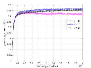
(a) Training curve of proposed RL-SCD algorithm for different penalty factor $\nu$.

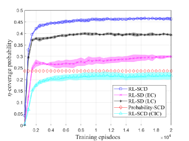
(b) Training curve of the proposed RL-SCD algorithm and baseline algorithms.

Figure 6: Training curve for the multiple EH sensor case.

Next, we show the simulation results of the multiple EH sensor case in Figs. 6 - 8. Figure 6 shows training curves, averaged over different seeds. In Fig. 6(a), the proposed RL-SCD algorithm can achieve the higher $\eta$-coverage probability with the penalty factor $\nu=1$, compared to those with $\nu=0$ and $\nu=2$, so we adopt $\nu=1$ for implementing the RL-based algorithms. Figure 6(b) presents the training curves of the proposed RL-SCD and baseline algorithms. From this figure, we observe that the $\eta$-coverage probability increases and converges as the training proceeds for RL-based algorithms. Note that the Probability-SCD is not a learning-based algorithm, there is no training curve. However, we present the $\eta$-coverage probability for this case as a line for the performance comparison purpose. We can observe that the proposed RL-SCD achieves higher performance than other algorithms. From Fig. 6(b), we can see that the RL-SCD (CIC) has lower performance even than Probability-SCD, which shows the importance of exploiting the temporal correlation of information for the sensing and computing decision.

\psfrag{Aratio}[Bc][Tc][0.8]{$\eta$-coverage probability, $\mathcal{P}_{\text{c}}(\eta)$}\psfrag{Sensornum}[tc][tc][0.8]{The number of sensors, $N_{\text{s}}$}\psfrag{MARL-based-DDDDDD}[tl][tl][0.7]{RL-SCD}\psfrag{MARL-EC}[tl][tl][0.7]{RL-SD (EC)}\psfrag{MARL-LC}[tl][tl][0.7]{RL-SD (LC)}\psfrag{Prob}[tl][tl][0.7]{Probability-SCD}\psfrag{CIC}[tl][tl][0.7]{RL-SCD (CIC)}\psfrag{Eta85}[tl][tl][0.65]{$\eta=0.85$}\psfrag{Eta90}[tl][tl][0.65]{$\eta=0.9$}\psfrag{EightSensors}[tc][tc][0.8]{$N_{\text{s}}=8$}\psfrag{FourteenSensors}[tc][tc][0.8]{$N_{\text{s}}=14$}\psfrag{1004}[tc][tc][0.65]{$\mathbb{E}_{t}[\phi_{\text{cov}}(t)]$}\psfrag{2004}[tc][tc][0.65]{Sensing ratio}\psfrag{3004}[tc][tc][0.65]{EC ratio}\psfrag{4004}[tc][tc][0.65]{$\mathbb{E}_{n,t}[\Delta_{n}^{\text{rx}}(t)]$(ms)}\includegraphics[width=195.12767pt]{Figures/Result_sensor_num_v3.eps}

(a) $\eta$-coverage probability of proposed and baseline algorithms according to $N_{\text{s}}$ for different $\eta$.

\psfrag{Aratio}[Bc][Tc][0.8]{$\eta$-coverage probability, $\mathcal{P}_{\text{c}}(\eta)$}\psfrag{Sensornum}[tc][tc][0.8]{The number of sensors, $N_{\text{s}}$}\psfrag{MARL-based-DDDDDD}[tl][tl][0.7]{RL-SCD}\psfrag{MARL-EC}[tl][tl][0.7]{RL-SD (EC)}\psfrag{MARL-LC}[tl][tl][0.7]{RL-SD (LC)}\psfrag{Prob}[tl][tl][0.7]{Probability-SCD}\psfrag{CIC}[tl][tl][0.7]{RL-SCD (CIC)}\psfrag{Eta85}[tl][tl][0.65]{$\eta=0.85$}\psfrag{Eta90}[tl][tl][0.65]{$\eta=0.9$}\psfrag{EightSensors}[tc][tc][0.8]{$N_{\text{s}}=8$}\psfrag{FourteenSensors}[tc][tc][0.8]{$N_{\text{s}}=14$}\psfrag{1004}[tc][tc][0.65]{$\mathbb{E}_{t}[\phi_{\text{cov}}(t)]$}\psfrag{2004}[tc][tc][0.65]{Sensing ratio}\psfrag{3004}[tc][tc][0.65]{EC ratio}\psfrag{4004}[tc][tc][0.65]{$\mathbb{E}_{n,t}[\Delta_{n}^{\text{rx}}(t)]$(ms)}\includegraphics[width=173.44865pt]{Figures/Result_sensor_num_ratio_noAoI_v2.eps}

(b) Average network coverage ratio $\mathbb{E}[\phi_{\text{cov}}(t)]$, sensing ratio, and EC ratio of RL-SCD and Probability-SCD for $N_{\text{s}}=8$ and $N_{\text{s}}=14$ when $\eta=0.9$.

Figure 7: Effect of the number of sensors, $N_{\text{s}}$, on the network performance.

Figure 7 shows the effect of the number of sensors, $N_{\text{s}}$, on the network performance. Firstly, Fig. 7(a) shows the $\eta$-coverage probability as a function of $N_{\text{s}}$ for different $\eta$. From this figure, we find that the $\eta$-coverage probability increases with $N_{\text{s}}$ because more sensors can cover larger area, as shown in (15). We can also observe that the proposed algorithm can achieve the higher $\eta$-coverage probability compared to the baseline algorithms even for high $\eta$.

In Fig. 7(b), we present the average network coverage ratio $\left(\mathbb{E}[\phi_{\text{cov}}(t)]\right)$, the ratios of performing (deciding) sensings or EC in each round, when $N_{\text{s}}=8$ and $N_{\text{s}}=14$. For Probability-SCD, we use the optimal $p_{\text{s}}^{*}$ and $p_{\text{e}}^{*}$, obtained in Section III, which are the same as the obtained sensing ratio and the EC ratio, respectively, in this case. Firstly, we observe that when the number of sensors is changed from $N_{\text{s}}=8$ to $N_{\text{s}}=14$, both the sensing ratio and the EC ratio become lower, to reduce the excessive energy consumption and the computation load at the EC server. From this figure, we can see that the EC ratio of RL-SCD is smaller than that of Probability-SCD. This is because, in RL-SCD, the AoI and the waiting time at the EC server are used as an observation to avoid the excessive waiting at the EC server. From Fig. 7(b), we can also see that the sensing ratio of RL-SCD is lower than that of Probability-SCD, which shows RL-SCD can achieve higher coverage ratio even with fewer sensing.

\psfrag{Aratio}[Bc][Tc][0.8]{$\eta$-coverage probability, $\mathcal{P}_{\text{c}}(\eta)$}\psfrag{ProcEnergy}[tc][tc][0.8]{Computing energy, $E_{\text{C}}$ (mJ) }\psfrag{MARL-based-DDDDDD}[tl][tl][0.7]{RL-SCD}\psfrag{MARL-EC}[tl][tl][0.7]{RL-SD (EC)}\psfrag{MARL-LC}[tl][tl][0.7]{RL-SD (LC)}\psfrag{Prob}[tl][tl][0.7]{Probability-based}\psfrag{CIC}[tl][tl][0.7]{RL-SCD (CIC)}\psfrag{LowDensity}[tl][tl][0.65]{$p_{\text{t}}=0.5$}\psfrag{HighDensity}[tl][tl][0.65]{$p_{\text{t}}=1$}\psfrag{ProcEnergy12}[tc][tc][0.8]{$E_{\text{C}}=12$ (mJ)}\psfrag{ProcEnergy28}[tc][tc][0.8]{$E_{\text{C}}=28$ (mJ)}\psfrag{1004}[tc][tc][0.65]{$\mathbb{E}_{t}[\phi_{\text{cov}}(t)]$}\psfrag{2004}[tc][tc][0.65]{Sensing ratio}\psfrag{3004}[tc][tc][0.65]{EC ratio}\psfrag{4004}[tc][tc][0.65]{$\mathbb{E}_{n,t}[\Delta_{n}^{\text{rx}}(t)]$(ms)}\includegraphics[width=195.12767pt]{Figures/Result_proc_energy.eps}

(a) $\eta$-coverage probability of proposed and baseline algorithms according to $E_{\text{C}}$ for different resource reuse probability $p_{\text{t}}$.

\psfrag{Aratio}[Bc][Tc][0.8]{$\eta$-coverage probability, $\mathcal{P}_{\text{c}}(\eta)$}\psfrag{ProcEnergy}[tc][tc][0.8]{Computing energy, $E_{\text{C}}$ (mJ) }\psfrag{MARL-based-DDDDDD}[tl][tl][0.7]{RL-SCD}\psfrag{MARL-EC}[tl][tl][0.7]{RL-SD (EC)}\psfrag{MARL-LC}[tl][tl][0.7]{RL-SD (LC)}\psfrag{Prob}[tl][tl][0.7]{Probability-based}\psfrag{CIC}[tl][tl][0.7]{RL-SCD (CIC)}\psfrag{LowDensity}[tl][tl][0.65]{$p_{\text{t}}=0.5$}\psfrag{HighDensity}[tl][tl][0.65]{$p_{\text{t}}=1$}\psfrag{ProcEnergy12}[tc][tc][0.8]{$E_{\text{C}}=12$ (mJ)}\psfrag{ProcEnergy28}[tc][tc][0.8]{$E_{\text{C}}=28$ (mJ)}\psfrag{1004}[tc][tc][0.65]{$\mathbb{E}_{t}[\phi_{\text{cov}}(t)]$}\psfrag{2004}[tc][tc][0.65]{Sensing ratio}\psfrag{3004}[tc][tc][0.65]{EC ratio}\psfrag{4004}[tc][tc][0.65]{$\mathbb{E}_{n,t}[\Delta_{n}^{\text{rx}}(t)]$(ms)}\includegraphics[width=173.44865pt]{Figures/Result_proc_energy_ratio_noAoI_v2.eps}

(b) Average network coverage ratio $\mathbb{E}[\phi_{\text{cov}}(t)]$, sensing ratio, and EC ratio of RL-SCD and Probability-SCD for $E_{\text{C}}=12$ mJ and $E_{\text{C}}=28$ mJ when $p_{\text{t}}=0.5$.

Figure 8: Effect of the computing energy, $E_{\text{C}}$, on the network performance.

Figure 8 shows the effect of the computing energy, $E_{\text{C}}$, on the network performance when $N_{\text{s}}=10$. Figure 8(a) shows the $\eta$-coverage probability of the proposed and baseline algorithms as a function of $E_{\text{C}}$ for different resource reuse probability $p_{\text{t}}$. From Fig. 8(a), we can see that the $\eta$-coverage probability decreases as $E_{\text{C}}$ increases, except for RL-SD (EC), which is not affected by $E_{\text{C}}$ as it does not perform LC. Moreover, the $\eta$-coverage probability becomes lower with $p_{\text{t}}=1$ compared to that with $p_{\text{t}}=0.5$ because higher $p_{\text{t}}$ means larger interference from other sensors, which increases the outage probability. However, RL-SCD can still achieve the higher $\eta$-coverage probability than other algorithms for all ranges of $E_{\text{C}}$ in Fig. 8.

Figure 8(b) shows the average network coverage ratio $\mathbb{E}[\phi_{\text{cov}}(t)]$, the sensing ratio, and the EC ratio when $E_{\text{C}}=12$ (mJ) and $E_{\text{C}}=28$ (mJ). From Fig. 8(b), we can see that when $E_{\text{C}}$ is changed from 12 (mJ) to 28 (mJ), the sensing ratio becomes lower and the EC ratio becomes higher, to prevent the excessive energy consumption for sensing and computing.

VI Conclusion

This paper proposes the probability-based SCD and the RL-based SCD algorithms for data freshness in the EC-enabled wireless sensor networks. Firstly, we propose the novel sensing coverage which is jointly affected by the spatial and the temporal correlation of information. Then, we design the probability-based SCD algorithm and derive the $\eta$-coverage probability in a closed form in the single pre-charged sensor case. Next, we obtain the optimal sensing and EC probabilities that maximize the $\eta$-coverage probability. We also design the RL-based SCD algorithm by training the policy of the sensors to take the real-time decision based on its observation in both the single pre-charged sensor and the multiple EH sensor cases. Through the simulation results, we first show the RL-based SCD algorithm can achieve the higher $\eta$-coverage probability than other baseline algorithms. We also provide some insights on the SCD, i.e., in the single pre-charged sensor case, as the distance between the sensor and the sink node increases, choosing the LC rather than EC, is helpful to enhance the $\eta$-coverage probability. In addition, in the multiple EH sensor case, we find that both the sensing ratio and EC ratio decrease with the number of sensors, while the EC ratio increases with the computing energy.

-A Proof of Lemma 1

The expected inter update time $\mathbb{E}[U_{k}]$ is represented as

$$\mathbb{E}[U_{k}]=\mathbb{E}\left[\tau_{\text{r}}-Z_{k-1}+X_{k}\right]\mathrel{\overset{\makebox[0.0pt]{{\tiny(a)}}}{=}}\tau_{\text{r}}-\mathbb{E}[Z_{k}]+\mathbb{E}[X_{k}],$$ (54)

where $Z_{k}$ is the time interval from the sensing instance to the successful update, and $X_{k}$ is the time interval from the first sensing decision time after the $(k-1)$-th successful update to the $k$-th successful update. Here, (a) holds because 1) $(k-1)$-th update and $k$-th update are independent and 2) $Z_{k-1}$ and $Z_{k}$ are identically distributed.

Since $\mathbb{E}[Z_{k}]$ and $\mathbb{E}[X_{k}]$ are affected by what computing model is used for the $k$-th successful update, i.e., $m_{k}\in\{\text{e},\ell\}$, both terms are expressed as the sum of conditional expectations $\mathbb{E}[Z_{k}|m_{k}]$ and $\mathbb{E}[X_{k}|m_{k}]$ as follows

$$\mathbb{E}[Z_{k}]=p_{\text{u}}(\text{e})\mathbb{E}[Z_{k}|\text{e}]+p_{\text{u}}(\ell)\mathbb{E}[Z_{k}|\ell],$$ (55)

$$\mathbb{E}[X_{k}]=p_{\text{u}}(\text{e})\mathbb{E}[X_{k}|\text{e}]+p_{\text{u}}(\ell)\mathbb{E}[X_{k}|\ell].$$ (56)

We first obtain $\mathbb{E}[Z_{k}|m_{k}]$. For given $m_{k}$, $Z_{k}$ is determined by the number of retransmissions attempted by the sensor until the transmission succeeds, denoted as $c$, so its distribution is modeled as the geometric distribution. $\mathbb{P}[Z_{k}|m_{k}]$ is given by

$$\mathbb{P}[Z_{k}=1+c+\tau_{k}|m_{k}]=\frac{p_{\textbf{o},{k}}^{c-1}\varrho_{1,k}}{\varrho_{\delta,k}}.$$ (57)

From (57), $\mathbb{E}[Z_{k}|m_{k}]$ is then obtained as

$$\begin{aligned} \mathbb{E}[Z_{k}|m_{k}]=\sum_{c=1}^{\delta}{(1+c+\tau_{k})}\frac{p_{\textbf{o},{k}}^{c-1}\varrho_{1,k}}{\varrho_{\delta,k}}=1+\tau_{k}+f_{\delta,k},\end{aligned}$$ (58)

where $f_{\delta,k}$ is defined at (29). From this, the expectation of the time interval from the sensing instance to the successful update $\mathbb{E}[Z_{k}]$ can be obtained.

Similarly, we obtain $\mathbb{E}[X_{k}|m_{k}]$. For given $m_{k}$, $X_{k}$ is affected by the number of rounds until the $k$-th update occurs, denoted as $Y_{k}$. When the $k$-th update occurs from $(k-1)$th update to $Y_{k}$ rounds after, the PMF $\mathbb{P}[Y_{k}=y|m_{k}]$ is given by

$$\begin{aligned} \mathbb{P}\left[Y_{k}=y|m_{k}\right]=p_{\delta}(1-p_{\delta})^{y-1}.\end{aligned}$$ (59)

The conditional expectation $\mathbb{E}[X_{k}|m_{k}]$ is then obtained as

$$\begin{aligned} \mathbb{E}[X_{k}|m_{k}]=&\sum_{y=1}^{\infty}\mathbb{P}[Y_{k}=y|m_{k}]\{(y-1)\tau_{\text{r}}+\mathbb{E}[Z_{k}|m_{k}]\}\\ =&\frac{\tau_{\text{r}}}{p_{\delta}}-\tau_{\text{r}}+1+\tau_{k}+f_{\delta,k}.\\ \end{aligned}$$ (60)

By substituting (26), (58) and (60) into (55) and (56), the expected inter-update time $\mathbb{E}[U_{k}]$ can be obtained as (23).

-B Proof of Lemma 2

To show the proof of the Lemma 2, we define the probability that the target AoI $v_{\text{th}}$ exists in the given ranges below, represented as

$$\hat{P}_{1}(v_{\text{th}}) =\mathbb{P}[v_{\text{th}}<Z_{k-1}|m_{k-1}],$$ (61)

$$\hat{P}_{2}(v_{\text{th}}) =\mathbb{P}[Z_{k-1}\leq v_{\text{th}}<\tau_{\text{r}}+X_{k}|(m_{k-1},m_{k})],$$ (62)

$$\hat{P}_{3}(v_{\text{th}}) =\mathbb{P}[\tau_{\text{r}}+X_{k}\leq v_{\text{th}}|(m_{k-1},m_{k})].$$ (63)

From (22), $g_{k}$ is jointly affected by $m_{k-1}$ and $m_{k}$. Hence, as shown in (25), we analyze the $\mathbb{E}[g_{k}]$ by splitting it into $m_{k-1}$ and $m_{k}$, i.e., $G(m_{k-1},m_{k})=\mathbb{E}[g_{k}|(m_{k-1},m_{k})]$, which is expressed as

$$\begin{aligned} G(m_{k-1},m_{k})\\ =\hat{P}_{1}(v_{\text{th}})\mathbb{E}&[\tau_{\text{r}}-Z_{k-1}+X_{k}|v_{\text{th}}<Z_{k-1},(m_{k-1},m_{k})]\\ +\hat{P}_{2}(v_{\text{th}})\mathbb{E}&\left[\tau_{\text{r}}+X_{k}-(\lfloor v_{\text{th}}\rfloor+1)|\right.\\ &\left.Z_{k-1}\leq v_{\text{th}}<\tau_{\text{r}}+X_{k},(m_{k-1},m_{k})\right].\end{aligned}$$ (64)

Since (64) depends on the range of $v_{\text{th}}$, $G(m_{k-1},m_{k})$ is obtained by following cases.

For $v_{\text{th}}<2+\tau_{k-1}$, the AoI at the sink node $\Delta^{\text{rx}}(t)$ always violates $v_{\text{th}}$ because the minimum time for the update with the sensed data is $2+\tau_{k-1}$ when the transmission succeeds at once, i.e., $c=1$. Hence, $v_{\text{th}}$ is always lower than $Z_{k-1}$, and we have

$$\begin{aligned} \hat{P}_{1}(v_{\text{th}})=1,\hat{P}_{2}(v_{\text{th}})=0,\hat{P}_{3}(v_{\text{th}})=0.\end{aligned}$$ (65)

By substituting (65) into (64), $G(m_{k-1},m_{k})$ is obtained as

$$\begin{aligned} G(m_{k-1},m_{k})&=\mathbb{E}[\tau_{\text{r}}-Z_{k-1}+X_{k}|(m_{k-1},m_{k})]\\ &=\tau_{\text{r}}-\mathbb{E}[Z_{k-1}|m_{k-1}]+\mathbb{E}[X_{k}|m_{k}],\end{aligned}$$ (66)

where the result is given in (32), case $v_{\text{th}}<v_{1}$.

For $2+\tau_{k-1}\leq v_{\text{th}}<1+\delta+\tau_{k-1}$, the maximum number of retransmissions is limited by $\lfloor v_{\text{th}}\rfloor-1-\tau_{k-1}$ to satisfy $v_{\text{th}}\geq Z_{k-1}$. Hence, we have

$$\begin{aligned} \hat{P}_{2}(v_{\text{th}})&=\sum_{c=1}^{\lfloor v_{\text{th}}\rfloor-1-\tau_{k-1}}\frac{p_{\textbf{o},{k-1}}^{c-1}\varrho_{1,k-1}}{\varrho_{\delta,k-1}}=\frac{\varrho_{\lfloor v_{\text{th}}\rfloor-1-\tau_{k-1},k-1}}{\varrho_{\delta,k-1}},\\ \hat{P}_{1}(v_{\text{th}})&=1-\hat{P}_{2}(v_{\text{th}}),\qquad\hat{P}_{3}(v_{\text{th}})=0.\end{aligned}$$ (67)

Since $\hat{P}_{1}(v_{\text{th}})+\hat{P}_{2}(v_{\text{th}})=1$, (64) can be rewritten as

$$\begin{aligned} G(m_{k-1},m_{k})&=\tau_{\text{r}}+\mathbb{E}[X_{k}|m_{k}]-\hat{P}_{2}(v_{\text{th}})(\lfloor v_{\text{th}}\rfloor+1)\\ &-\hat{P}_{1}(v_{\text{th}})\mathbb{E}[Z_{k-1}|v_{\text{th}}<Z_{k-1},m_{k-1}].\end{aligned}$$ (68)

Here, $\mathbb{E}[Z_{k-1}|v_{\text{th}}<Z_{k-1},m_{k-1}]$ is represented as

$$\begin{aligned} &\mathbb{E}[Z_{k-1}|v_{\text{th}}<Z_{k-1},m_{k-1}]\\ &=\sum_{c=\lfloor v_{\text{th}}\rfloor-\tau_{k-1}}^{\delta}(1+c+\tau_{k-1})\frac{p_{\textbf{o},{k-1}}^{c-1}\varrho_{1,k-1}}{p_{\textbf{o},{k-1}}^{\lfloor v_{\text{th}}\rfloor-1-\tau_{k-1}}-p_{\textbf{o},{k-1}}^{\delta}}\\ &=1+\tau_{k-1}+\frac{1}{\varrho_{1,k-1}}\\ &+\frac{(\lfloor v_{\text{th}}\rfloor-1-\tau_{k-1})p_{\textbf{o},{k-1}}^{\lfloor v_{\text{th}}\rfloor-1-\tau_{k-1}}-\delta p_{\textbf{o},{k-1}}^{\delta}}{p_{\textbf{o},{k-1}}^{\lfloor v_{\text{th}}\rfloor-1-\tau_{k-1}}-p_{\textbf{o},{k-1}}^{\delta}}.\end{aligned}$$ (69)

By substituting (67) and (69) into (68), $G(m_{k-1},m_{k})$ can be obtained where the result is given in (32), case $v_{1}\leq v_{\text{th}}<v_{2}$.

For $1+\delta+\tau_{k-1}\leq v_{\text{th}}<\tau_{\text{r}}+2+\tau_{k}$, we have

$$\hat{P}_{1}(v_{\text{th}})=0,\hat{P}_{2}(v_{\text{th}})=1,\hat{P}_{3}(v_{\text{th}})=0.$$ (70)

By substituting (70) into (64), $G(m_{k-1},m_{k})$ can be obtained where the result is given in (32), case $v_{2}\leq v_{\text{th}}<v_{3,y=1}$.

For $y\tau_{\text{r}}+2+\tau_{k}\leq v_{\text{th}}<y\tau_{\text{r}}+1+\delta+\tau_{k},\;y=1,2,\cdots,$ $v_{\text{th}}$ is always larger than $Z_{k-1}$, i.e., $\hat{P}_{1}(v_{\text{th}})=0$. In addition, $\tau_{\text{r}}+X_{k}\leq v_{\text{th}}$ is satisfied when the update succeeds within $(y-1)$ rounds or within $\kappa_{k}(y)$ slots at $y$-th round, where $\kappa_{k}(y)$ is defined in (31). Hence, we have

$$\begin{aligned} \hat{P}_{1}(v_{\text{th}})&=0,\\ \hat{P}_{3}(v_{\text{th}})&=1+(1-p_{\delta})^{y-1}\left(p_{\delta}\frac{\varrho_{\kappa_{k}(y),k}}{\varrho_{\delta,k}}-1\right),\\ \hat{P}_{2}(v_{\text{th}})&=1-\hat{P}_{3}(v_{\text{th}})\\ &=-(1-p_{\delta})^{y-1}\left(p_{\delta}\frac{\varrho_{\kappa_{k}(y),k}}{\varrho_{\delta,k}}-1\right).\end{aligned}$$ (71)

By substituting (73) into (64), $G(m_{k-1},m_{k})$ is given as

$$\begin{aligned} &G(m_{k-1},m_{k})\\ &=\hat{P}_{2}(v_{\text{th}})\mathbb{E}[\tau_{\text{r}}+X_{k}-(\lfloor v_{\text{th}}\rfloor+1)|Z_{k-1}\leq v_{\text{th}}<\tau_{\text{r}}+X_{k}]\\ &=p_{\delta}(1-p_{\delta})^{y-1}\sum_{c=\kappa_{k}(y)+1}^{\delta}\{(y-1)\tau_{\text{r}}+1+c+\tau_{k}\}\\ &\times\frac{p_{\textbf{o},{k}}^{c-1}\varrho_{1,k}}{\varrho_{\delta,k}}+\sum_{Y=y}^{\infty}p_{\delta}(1-p_{\delta})^{Y}\{Y\tau_{\text{r}}+\mathbb{E}[Z_{k}|m_{k}]\}\\ &-(1-p_{\delta})^{y-1}\left(p_{\delta}\frac{\varrho_{\kappa_{k}(y),k}}{\varrho_{\delta,k}}-1\right)\{\tau_{\text{r}}-(\lfloor v_{\text{th}}\rfloor+1)\},\end{aligned}$$ (72)

where the result is given in (32), case $v_{3}(y)\leq v_{\text{th}}<v_{4}(y)$.

For $y\tau_{\text{r}}+1+\delta+\tau_{k}\leq v_{\text{th}}<(y+1)\tau_{\text{r}}+2+\tau_{k},\;y=1,2,\cdots$, $\hat{P}_{1}(v_{\text{th}})=0$, similar to the above case. In addition, $\tau_{\text{r}}+X_{k}\leq v_{\text{th}}$ is satisfied when the update succeeds within $y$ rounds, so we have

$$\begin{aligned} \hat{P}_{1}(v_{\text{th}})&=0,\quad\hat{P}_{3}(v_{\text{th}})=\sum_{Y=1}^{y}p_{\delta}(1-p_{\delta})^{Y-1}=1-(1-p_{\delta})^{y},\\ \hat{P}_{2}(v_{\text{th}})&=1-\hat{P}_{3}(v_{\text{th}})=(1-p_{\delta})^{y}.\end{aligned}$$ (73)

By substituting (73) into (64), $G(m_{k-1},m_{k})$ is obtained as

$$\begin{aligned} &G(m_{k-1},m_{k})\\ &=\sum_{Y=y+1}^{\infty}p_{\delta}(1-p_{\delta})^{Y-1}\{(Y-1)\tau_{\text{r}}+\mathbb{E}[Z_{k}|m_{k}]\}\\ &+(1-p_{\delta})^{y}\{\tau_{\text{r}}-(\lfloor v_{\text{th}}\rfloor+1)\},\end{aligned}$$ (74)

where the result is given in (32), case $v_{4}(y)\leq v_{\text{th}}<v_{3}(y+1)$.

From (32), the expected violation time $\mathbb{E}[g_{k}]$ can be obtained by (25). Finally, from (20), the AoI violation probability can be expressed by dividing the obtained $\mathbb{E}[g_{k}]$ into $\mathbb{E}[U_{k}]$.

References

- [1] S. Yun, D. Kim, C. Park, and J. Lee, “Joint sensing and computation decision for age of information-sensitive wireless networks: A deep reinforcement learning approach,” in Proc. IEEE Glob. Commun. Conf. (GLOBECOM), Kuala Lumpur, Malaysia, Dec. 2023, pp. 1–6.
- [2] O. Vermesan and P. Friess, Internet of things: converging technologies for smart environments and integrated ecosystems. River publishers, 2013.
- [3] J. Yick, B. Mukherjee, and D. Ghosal, “Wireless sensor network survey,” Comput. Netw., vol. 52, no. 12, pp. 2292–2330, Aug. 2008.
- [4] W. Shi, J. Cao, Q. Zhang, Y. Li, and L. Xu, “Edge computing: vision and challenges,” IEEE Internet Things J., vol. 3, no. 5, pp. 637–646, Jun. 2016.
- [5] Y. Mao, C. You, J. Zhang, K. Huang, and K. B. Letaief, “A survey on mobile edge computing: the communication perspective,” IEEE Commun. Surveys Tuts., vol. 19, no. 4, pp. 2322–2358, FourthQuarter 2017.
- [6] W. Liu, X. Zhou, S. Durrani, H. Mehrpouyan, and S. D. Blostein, “Energy harvesting wireless sensor networks: Delay analysis considering energy costs of sensing and transmission,” IEEE Trans. Wirel. Commun., vol. 15, no. 7, pp. 4635–4650, Mar. 2016.
- [7] I. Krikidis, “Average age of information in wireless powered sensor networks,” IEEE Commun. Lett., vol. 8, no. 2, pp. 628–631, Apr. 2019.
- [8] B. T. Bacinoglu and E. Uysal-Biyikoglu, “Scheduling status updates to minimize age of information with an energy harvesting sensor,” in Proc. IEEE Int. Symp. Inf. Theory (ISIT), Aachen, Germany, Jun. 2017, pp. 1–5.
- [9] X. Wu, J. Yang, and J. Wu, “Optimal status update for age of information minimization with an energy harvesting source,” IEEE Trans. Green Commun. and Netw., vol. 2, no. 1, pp. 193–204, Nov. 2017.
- [10] E. T. Ceran, D. Gündüz, and A. György, “Reinforcement learning to minimize age of information with an energy harvesting sensor with HARQ and sensing cost,” in Proc. IEEE Conf. Comput. Commun. Workshops (INFOCOM WKSHPS), Paris, France, Apr. 2019, pp. 1–6.
- [11] M. Moltafet, M. Leinonen, and M. Codreanu, “On the age of information in multi-source queueing models,” IEEE Trans. Commun., vol. 68, no. 8, pp. 5003–5017, May 2020.
- [12] I. Kadota, A. Sinha, and E. Modiano, “Optimizing age of information in wireless networks with throughput constraints,” in Proc. IEEE Conf. Comput. Commun. (INFOCOM), Honolulu,HI,USA, Apr. 2018, pp. 1–9.
- [13] J. Hribar, M. Costa, N. Kaminski, and L. A. DaSilva, “Using correlated information to extend device lifetime,” IEEE Internet Things J., vol. 6, no. 2, pp. 2439–2448, Apr. 2019.
- [14] J. Hribar, A. Marinescu, A. Chiumento, and L. A. DaSilva, “Energy aware deep reinforcement learning scheduling for sensors correlated in time and space,” IEEE Internet Things J., pp. 1–13, Sep. 2021.
- [15] S. Kaul, R. Yates, and M. Gruteser, “Real-time status: How often should one update?” in Proc. IEEE Conf. Comput. Commun. (INFOCOM), Orlando, FL, USA, Mar. 2012, pp. 2731–2735.
- [16] F. Xu, H. Ye, F. Yang, and C. Zhao, “Software defined mission-critical wireless sensor network: Architecture and edge offloading strategy,” IEEE Access, vol. 7, pp. 10 383–10 391, Jan. 2019.
- [17] S. Jošilo and G. Dán, “Computation offloading scheduling for periodic tasks in mobile edge computing,” IEEE ACM Trans. Netw., vol. 28, no. 2, pp. 667–680, Feb. 2020.
- [18] X. Ma, A. Zhou, Q. Sun, and S. Wang, “Freshness-aware information update and computation offloading in mobile-edge computing,” IEEE Internet Things J., vol. 8, no. 16, pp. 13 115–13 125, May 2021.
- [19] R. Li, Q. Ma, J. Gong, Z. Zhou, and X. Chen, “Age of processing: Age-driven status sampling and processing offloading for edge-computing-enabled real-time IoT applications,” IEEE Internet Things J., vol. 8, no. 19, pp. 14 471–14 484, Mar. 2021.
- [20] C. Xu, H. H. Yang, X. Wang, and T. Q. Quek, “Optimizing information freshness in computing-enabled IoT networks,” IEEE Internet Things J., vol. 7, no. 2, pp. 971–985, Oct. 2019.
- [21] G. B. Tayeh, A. Makhoul, C. Perera, and J. Demerjian, “A spatial-temporal correlation approach for data reduction in cluster-based sensor networks,” IEEE Access, vol. 7, pp. 50 669–50 680, Apr. 2019.
- [22] B. Wang, X. Deng, W. Liu, L. T. Yang, and H.-C. Chao, “Confident information coverage in sensor networks for field reconstruction,” IEEE Wirel. Commun., vol. 20, no. 6, pp. 74–81, 2013.
- [23] M. Haenggi, R. K. Ganti et al., “Interference in large wireless networks,” Found. and Trends Netw., vol. 3, no. 2, pp. 127–248, Nov. 2009.
- [24] X. Chen, L. Jiao, W. Li, and X. Fu, “Efficient multi-user computation offloading for mobile-edge cloud computing,” IEEE ACM Trans. Netw., vol. 24, no. 5, pp. 2795–2808, 2015.
- [25] H. ElSawy and E. Hossain, “On stochastic geometry modeling of cellular uplink transmission with truncated channel inversion power control,” IEEE Trans. Wirel. Commun., vol. 13, no. 8, pp. 4454–4469, Apr. 2014.
- [26] T. D. Novlan, H. S. Dhillon, and J. G. Andrews, “Analytical modeling of uplink cellular networks,” IEEE Trans. Wirel. Commun., vol. 12, no. 6, pp. 2669–2679, 2013.
- [27] F. Baccelli and B. Błaszczyszyn, “Stochastic geometry and wireless networks: Volume I theory,” 2009.
- [28] D. Tse and P. Viswanath, Fundamentals of wireless communication. Cambridge university press, 2005.
- [29] Y. Zhao, R. Adve, and T. J. Lim, “Improving amplify-and-forward relay networks: optimal power allocation versus selection,” in Proc. IEEE Int. Symp. Inf. Theory (ISIT), 2006, pp. 1234–1238.
- [30] E. Yoneki and J. Bacon, “A survey of wireless sensor network technologies,” UCAM-CL-TR-646, Sep. 2005.
- [31] M. A. M. Vieira, C. N. Coelho, D. j. da Silva, and J. M. da Mata, “Survey on wireless sensor network devices,” in Proc. IEEE Conf. Emerg. Technol. and Fact. Autom. (ETFA), vol. 1, Sep. 2003, pp. 537–544.
- [32] Y. Luo, L. Pu, G. Wang, and Y. Zhao, “RF energy harvesting wireless communications: RF environment, device hardware and practical issues,” Sensors, vol. 19, no. 13, p. 3010, Jul. 2019.
- [33] P. Lee, Z. A. Eu, M. Han, and H.-P. Tan, “Empirical modeling of a solar-powered energy harvesting wireless sensor node for time-slotted operation,” in Proc. IEEE Wireless Commun. and Netw. Conf. (WCNC), Mar. 2011, pp. 179–184.
- [34] M. L. Stein, “Space-time covariance functions,” J. Am. Statist. Assoc., vol. 100, no. 469, pp. 310–321, Dec. 2005.
- [35] J. Kim, M. Kim, M.-S. Kim, and J. Lee, “Ensuring data freshness in wireless monitoring networks: Age-of-information sensitive coverage and energy efficiency perspectives,” IEEE Internet Things J., vol. 10, no. 14, pp. 12 811–12 825, Mar. 2023.
- [36] J. P. Champati, H. Al-Zubaidy, and J. Gross, “On the distribution of AoI for the GI/GI/1/1 and GI/GI/1/2* systems: Exact expressions and bounds,” in Proc. IEEE Conf. Comput. Commun. (INFOCOM), Paris, France, Apr. 2019, pp. 1–9.
- [37] R. Lowe, Y. Wu, A. Tamar, J. Harb, P. Abbeel, and I. Mordatch, “Multi-agent actor-critic for mixed cooperative-competitive environments,” in Proc. Neural. Inf. Process. (NIPS), Long Beach, CA, USA, Dec. 2017, pp. 1–12.
- [38] E. Jang, S. Gu, and B. Poole, “Categorical reparameterization with gumbel-softmax,” in Proc. Int. Conf. Learn. Represent. (ICLR), Toulon, France, Apr. 2017, pp. 1–12.
- [39] N. Naderializadeh, J. J. Sydir, M. Simsek, and H. Nikopour, “Resource management in wireless networks via multi-agent deep reinforcement learning,” IEEE Trans. Wirel. Commun., vol. 20, no. 6, pp. 3507–3523, 2021.
- [40] J. Chen, S. Chen, Q. Wang, B. Cao, G. Feng, and J. Hu, “iRAF: A deep reinforcement learning approach for collaborative mobile edge computing IoT networks,” IEEE Internet Things J., vol. 6, no. 4, pp. 7011–7024, 2019.
- [41] T. Zhang, Z. Wang, Y. Liu, W. Xu, and A. Nallanathan, “Joint resource, deployment, and caching optimization for AR applications in dynamic UAV NOMA networks,” IEEE Trans. Wirel. Commun., vol. 21, no. 5, pp. 3409–3422, 2021.
- [42] J. Gong, X. Chen, and X. Ma, “Energy-age tradeoff in status update communication systems with retransmission,” in Proc. IEEE Glob. Commun. Conf. (GLOBECOM), Abu Dhabi, UAE, Dec. 2018, pp. 1–6.
- [43] S. Kumar, T. H. Lai, and J. Balogh, “On k-coverage in a mostly sleeping sensor network,” in Proc. annu. Int. Conf. Mob. Comput. Netw. (MobiCom), Philadelphia,PA, USA, Sep. 2004, pp. 1–15.
- [44] Z. Liao, J. Peng, J. Huang, J. Wang, J. Wang, P. K. Sharma, and U. Ghosh, “Distributed probabilistic offloading in edge computing for 6g-enabled massive internet of things,” IEEE Internet Things J., vol. 8, no. 7, pp. 5298–5308, Oct. 2020.