Spectral Clustering for Discrete Distributions

Abstract.

Discrete distribution clustering (D2C) was often solved by Wasserstein barycenter methods. These methods are under a common assumption that clusters can be well represented by barycenters, which may not hold in many real applications. In this work, we propose a simple yet effective framework based on spectral clustering and distribution affinity measures (e.g., maximum mean discrepancy and Wasserstein distance) for D2C. To improve the scalability, we propose to use linear optimal transport to construct affinity matrices efficiently on large datasets. We provide theoretical guarantees for the success of the proposed methods in clustering distributions. Experiments on synthetic and real data show that our methods outperform the baselines largely in terms of both clustering accuracy and computational efficiency.

1. Introduction and Related Work

Clustering is a fundamental task in machine learning. A variety of clustering methods have been developed in the past decades (Shi and Malik, 2000; Jain et al., 1999; Ng et al., 2001; Parsons et al., 2004; Kriegel et al., 2009; Elhamifar and Vidal, 2013; Zhang et al., 2015; Campello et al., 2015; Pandove et al., 2018; Fan, 2021; Cai et al., 2022; Fan et al., 2022; Sun et al., 2023). Traditional clustering methods focus on clustering individual samples typically represented as vectors (Ng et al., 2001; Parsons et al., 2004; Campello et al., 2015; Pandove et al., 2018; Cai et al., 2022). However, many data are not intrinsically vectors, e.g., images and documents, which are discrete distributions. The discrete distribution is a well-adopted way to depict the characteristics of a batch of data. To cluster discrete distributions, one may consider representing each batch of data as a vector (e.g., the mean value of the batch), which will lose important information about the batch and lead to unsatisfactory clustering results. Alternatively, one may cluster all the data points without considering the batch condition and use post-processing to obtain the partition over batches, which does not explicitly exploit the distribution of each batch in the learning stage and may not provide high clustering accuracy. Therefore, finding an efficient and effective clustering method for discrete distributions is essential rather than using pre-processing or post-processing heuristics.

A few methods based on a framework called D2-Clustering (Li and Wang, 2008) have been developed for discrete distribution clustering. D2-Clustering adopted the well-accepted criterion of minimizing the total within-cluster variation under the Wasserstein distance, similar to Lloyd’s K-means for vectors under Euclidean distance. The Wasserstein distance, which arises from the idea of optimal transport (Villani, 2008), captures meaningful geometric features between probability measures and can be used to compare two discrete distributions. D2-Clustering computes a centroid called Wasserstein barycenter (Agueh and Carlier, 2011), also a discrete distribution, to summarize each cluster of discrete distributions. However, the Wasserstein distance has no closed-form solution. Given two discrete distributions, each with $m$ support points, the Wasserstein distance can only be solved with a worst-case time complexity $O(m^{3}\log m)$ (Orlin, 1988). D2-Clustering’s high computational cost limits its application to large datasets. Benamou et al. (2015) used iterative Bregman projections (IBP) to solve an approximation to the Wasserstein barycenter after adding an entropy regularization term. IBP is highly efficient with a memory complexity $O((m+\bar{m})N)$ for $N$ distributions with shared supports (e.g. histograms), and $O(m\bar{m}N)$ time complexity per iteration, where $\bar{m}$ is the number of support points of the barycenter. If distributions do not share the support set, IBP has the memory complexity $O(m\bar{m}N)$. (Ye et al., 2017b) developed a modified Bregman ADMM (B-ADMM) approach for computing approximate discrete Wasserstein barycenters. B-ADMM approach is of the same time complexity but requires $O(m\bar{m}N)$ memory complexity even if distributions have the same support set. But B-ADMM requires little hyper-parameter tuning, works well with single-precision floats, and performs better than IBP with sparse supports, making it more desirable for machine learning tasks.

Despite the successful applications, the D2-based methods mentioned above have the following limitations.

1. Support sparsity Anderes et al. (2016) proved that the actual support of the true barycenter is highly sparse, with cardinality $m$ at most $\bar{m}N$. Solving the true discrete barycenter quickly is intractable even for a small number of distributions that contains a small number of support points. To achieve good approximation, we need to carefully select a large number of representative initial support points and allow the support points in a barycenter to adjust positions every $\tau$ iterations, which imposes difficulties for implementation.

2. High computational cost In each iteration of D2-Clustering, one has to compute $K$ barycenters. Thus the computational cost is large if $K$ and the number of iterations are large. Please refer to the time complexity and cost comparisons in Table 5 and Table 6, respectively.

3. Assumption violation D2-Clustering assumes the distributions concentrate at some centroids, which may not hold in real applications. On the other hand, global distances may not reveal the intrinsic structures of distributions. Please refer to the intuitive example in Figure 1.

4. Lacking theoretical guarantees The study on theoretical guarantees for the success of D2-Clustering is very limited. It is unclear under what conditions we can cluster the distributions correctly.

This work aims to address the aforementioned four issues. Our contributions are two-fold.

• We propose a new framework for discrete distribution clustering based on spectral clustering and distribution affinity measures (e.g., Maximum Mean Discrepancy and Wasserstein distance). Our new methods are extremely easy to implement and do not need careful initialization.

• We provide theoretical guarantees for the consistency and correctness of clustering for our proposed methods. The theoretical results provide strong support for practical applications.

We evaluate our methods’ accuracy, robustness, and scalability compared to baselines on both synthetic and real data. Our methods outperform the baselines remarkably.

Notations  Let $\Omega$ be an arbitrary space, $P(\Omega)$ be the set of Borel probability measures on $\Omega$. $|\Omega|$ is the diameter $\sup\{\|\mathbf{x}-\mathbf{x}^{\prime}\||~{}\mathbf{x},\mathbf{x}^{\prime}\in\Omega\}$. Let $\mathcal{C}(\Omega)$ be the set of continuous functions on $\Omega$. For any $\mathbf{x}\in\Omega$, $\delta_{\mathbf{x}}$ is the Dirac unit mass on $\mathbf{x}$. $\mathbf{X}=(\mathbf{x}_{1},\dots,\mathbf{x}_{n})$ and $\mathbf{Y}=(\mathbf{y}_{1},\dots,\mathbf{y}_{m})$ are two sets of points in $\Omega$ (WLOG, we assume $m=n$ to simplify notations). $\mathbf{x}_{i}$ and $\mathbf{y}_{i}$ are also called the support points of the distributions. $\Sigma_{n}:=\{\mathbf{x}\in\mathbb{R}^{n}_{+}:\mathbf{x}^{\top}\mathbf{1}_{n}=1\}$ is $n$-dimensional probability simplex. All the sample points are in $\mathbb{R}^{d}$. $\mathbf{X}_{i}=(\mathbf{x}_{1},\mathbf{x}_{2},\ldots,\mathbf{x}_{m_{i}})^{\top}\in\mathbb{R}^{m_{i}\times d}$ are independently drawn from $\mu_{i}$, $i=1,2,\ldots,N$. We use $\mathbf{D}$, $\mathbf{A}$, and $\mathbf{L}$ to denote distance, adjacency, and Laplacian matrices respectively. $\|\cdot\|_{\infty}$ denotes the maximum element of matrix.

2. Preliminary Knowledge

Measuring the divergence or distance between distributions is a fundamental problem in statistics, information theory, and machine learning (Liese and Vajda, 2006; Kolouri et al., 2017). Well-known measurements include Kullback-Liebler (KL) divergence, $\chi^{2}$-divergence, MMD (Gretton et al., 2006, 2012), Wasserstein distance (Panaretos and Zemel, 2019), Sinkhorn divergences (Cuturi, 2013), etc. We briefly introduce MMD, Wasserstein distance, and Sinkhorn divergences in the following context because they are widely used in comparing discrete distributions and will be used in our proposed clustering methods.

2.1. Maximum Mean Discrepancy

Consider two probability distributions $\alpha,\beta$, the maximum mean discrepacy associated to a kernel $k$ is defined by

(1) $$\operatorname{MMD}(\alpha,\beta):=\mathbb{E}_{\alpha\otimes\alpha}[k(X,X^{\prime})]+\mathbb{E}_{\beta\otimes\beta}[k(Y,Y^{\prime})]-2\mathbb{E}_{\alpha\otimes\beta}[k(X,Y)].$$

An empirical estimation of MMD with finite samples $\mathbf{X},\mathbf{Y}$ from distributions $\alpha,\beta$ is defined by

(2) $$\widehat{\operatorname{MMD}}^{2}(\mathbf{X},\mathbf{Y}):=\frac{1}{m(m-1)}\sum_{i=1}^{m}\sum_{j\neq i}^{m}k\left(\mathbf{x}_{i},\mathbf{x}_{j}\right)+\frac{1}{m(m-1)}\sum_{i=1}^{m}\sum_{j\neq i}^{m}k\left(\mathbf{y}_{i},\mathbf{y}_{j}\right)-\frac{2}{m^{2}}\sum_{i=1}^{m}\sum_{j=1}^{m}k\left(\mathbf{x}_{i},\mathbf{y}_{j}\right).$$

2.2. Optimal Transport

Optimal Transport (OT) has been used extensively in recent years as a powerful tool to compare distributions. Consider two probability measures $\alpha,\beta\in P(\Omega)$, the Kantorovich formulation (Kantorovich, 1960) of OT between $\alpha$ and $\beta$ is

(3) $$W(\alpha,\beta)=\min_{\pi\in\Pi(\alpha,\beta)}\int_{\Omega^{2}}c(x,y)\mathrm{~{}d}\pi(x,y),$$

where $\Pi(\alpha,\beta)$ is the set of all probability measures on $\Omega^{2}$ that has marginals $\alpha$ and $\beta$. Elements $\pi\in\Pi(\alpha,\beta)$ are called couplings of $\alpha$ and $\beta$. $c(x,y)$ is the cost function representing the cost to move a unit of mass from $x$ to $y$. The famous $k$-Wasserstein distance is defined as

(4) $$W_{k}(\alpha,\beta)=\left(\min_{\pi\in\Pi(\alpha,\beta)}\int_{\Omega^{2}}\|x-y\|^{k}\mathrm{~{}d}\pi(x,y)\right)^{1/k}.$$

In practice, we usually use empirical discrete measures. For $\hat{\alpha}=\sum_{i=1}^{m}a_{i}\delta_{x_{i}}$ and $\hat{\beta}=\sum_{i=1}^{m}b_{i}\delta_{y_{i}}$ where $\mathbf{a}\in\Sigma_{m}$ and $\mathbf{b}\in\Sigma_{m}$, the optimal transport problem is

(5) $$\hat{W}(\hat{\alpha},\hat{\beta}):=\min_{\mathbf{P}\in U(a,b)}\langle\mathbf{P},\mathbf{C}\rangle,$$

where $U(\mathbf{a},\mathbf{b})=\left\{\mathbf{P}\in\mathbb{R}_{+}^{m\times m}\mid\mathbf{P}\mathbf{1}_{m}=\mathbf{a},\mathbf{P}^{T}\mathbf{1}_{m}=\mathbf{b}\right\}$ is named as transport polytope and $\mathbf{C}$ is denotes cost matrix.

2.3. Sinkhorn Divergences

To ease the agony of the high computation cost of OT, Cuturi (2013) proposed a smooth formulation of the classic optimal transport problem with an entropic regularization term. It was shown that the resulting optimum is also a distance, which can be computed through Sinkhorn’s matrix scaling algorithm at a cost of $O(m^{2})$ per iteration (Cuturi, 2013).

We use the relative entropy of the transport plan with respect to the product measure $\alpha\otimes\beta$ (Genevay et al., 2016). Let $H(\pi|\alpha\otimes\beta):=-\int_{\Omega^{2}}\log\left(\frac{\mathrm{~{}d}\pi(x,y)}{\mathrm{~{}d}\alpha(x)\mathrm{~{}d}\beta(y)}\right)\mathrm{~{}d}\pi(x,y)$. The relative entropy regularized OT can be formulated as

(6) $$W_{\varepsilon}(\alpha,\beta):=\min_{\pi\in\Pi(\alpha,\beta)}\int_{\Omega^{2}}c(x,y)\mathrm{~{}d}\pi(x,y)+\varepsilon H(\pi|\alpha\otimes\beta)$$

The empirical measure of regularized transport problem can be defined similarly

(7) $$\hat{W}_{\varepsilon}(\hat{\alpha},\hat{\beta}) :=\min_{\mathbf{P}\in U(a,b)}\langle\mathbf{P},\mathbf{C}\rangle+\varepsilon H(\mathbf{P}|\hat{\alpha}\otimes\hat{\beta}),$$

where $H(\mathbf{P}|\hat{\alpha}\otimes\hat{\beta})=-\sum_{i=1}^{m}\sum_{j=1}^{m}p_{ij}\log\frac{p_{ij}}{a_{i}b_{j}}$. The distance $W_{\varepsilon}(\alpha,\beta)$ is well-known as the regularized optimal transport distance or dual-Sinkhorn divergence (Cuturi, 2013; Genevay et al., 2018).

2.4. Wasserstein Barycenter and D2-Clustering

Li and Wang (2008) first proposed the discrete distribution (D2) clustering method for automatic picture annotation. D2 clustering adopts the same spirit as K-means clustering. Instead of vectors, D2 clustering aims at finding clusters for distributions. It computes a principled centroid to summarize each cluster of data. The centroids computed from those distribution clusters, also represented by discrete distributions, are known as Wasserstein barycenter (WB). Consider a set of discrete distributions $\{\nu_{i},i=1,\dots,N\}$, the WB is the solution of the following problem

(8) $$\min_{\mu}\sum_{i=1}^{N}W^{2}(\mu,\nu_{i}).$$

The goal of D2 clustering is to find a set of such centroid distributions $\{\mu_{k},k=1,\dots,K\}$ such that the total within-cluster variation is minimized:

(9) $$\min_{\{\mu_{k}\}}\sum_{k=1}^{K}\sum_{i\in C_{k}}W^{2}(\mu_{k},\nu_{i})$$

where $C_{k}$ is cluster $k$ and $\mu_{k}$ is the WB of $C_{k}$.

3. Discrete Distribution Spectral Clustering

3.1. Motivation and Problem Formulation

As mentioned in Section 2.4, existing methods of clustering discrete distributions are mainly based on Wasserstein barycenters. This means these methods require a common assumption that the members in each distribution can be well determined by the Wasserstein distances to the barycenters. Hence, like K-means, these methods are distance-based methods. In real applications, the distributions may not concentrate at some so-called “centers” but lie in some irregular shapes or on multiple manifolds. We should use connectivity-based clustering methods such as spectral clustering in these cases. Figure 1 shows an intuitive comparison between distance-based clustering and connectivity-based clustering of distributions, where ellipses and rectangles denote distributions. We make the following formal definition.

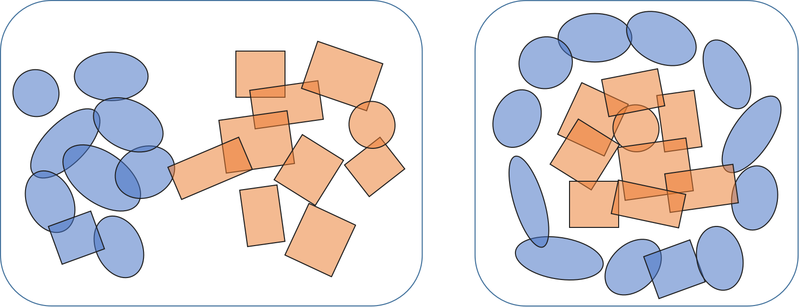
Figure 1. An intuitive comparison between distance-based (left plot) clustering and connectivity-based (right plot) clustering of distributions. Ellipses and rectangles denote distributions. The two clusters are marked in different colors.

Definition 3.1 (Connectivity-based distribution clustering).

Given $N$ distributions $\mu_{1},\mu_{2},\ldots,\mu_{N}$ in $\mathbb{R}^{d}$ that can be organized into $K$ groups $C_{1},C_{2},\ldots,C_{K}$. Let $\text{dist}(\cdot,\cdot)$ be a distance metric between two distributions and use it to construct a $\tau$ nearest neighbor ($\tau$-NN) graph $G=(V,E)$ over the $N$ distributions, on which each node corresponds a distribution. We assume that the following properties hold for the graph: 1) $G$ has $K$ connected components; 2) $(i,j)\notin E$ if $\mu_{i}$ and $\mu_{j}$ are not in the same group.

The two properties in the definition are sufficient to guarantee that partitioning the graph into $K$ groups yields correct clustering for the $N$ distributions. Note that the definition is actually a special case of connectivity-based clustering because there are many other approaches or principles for constructing a graph. In addition, it is possible that a correct clustering can be obtained even when some $(i,j)\in E$ but $\mu_{i}$ and $\mu_{j}$ are not in the same group. In this work, we aim to solve the following problem.

Definition 3.2 (Connectivity-based discrete distribution clustering).

Based on Definition 3.1, suppose $\mathbf{X}_{i}=[\mathbf{x}_{1},\mathbf{x}_{2},\ldots,\mathbf{x}_{m_{i}}]^{\top}\in\mathbb{R}^{m_{i}\times d}$ are independently drawn from $\mu_{i}$, $i=1,2,\ldots,N$. The goal is to partition $\mathbf{X}_{1},\mathbf{X}_{2},\ldots,\mathbf{X}_{N}$ into $K$ groups corresponding to $C_{1},C_{2},\ldots C_{K}$ respectively.

3.2. Algorithm

To solve the problem defined in Definition 3.2, we proposed to use MMD (Section 2.1), Wasserstein distance (Section 2.2), or Sinkhorn divergence (Section 2.3) to estimate a distance matrix $\mathbf{D}$ between the $N$ distributions:

(10) $$D_{ij}=\text{dist}(\mathbf{X}_{i},\mathbf{X}_{j}),\quad(i,j)\in[N]\times[N].$$

Then we convert this distance matrix $\mathbf{D}$ to an adjacency matrix $\mathbf{A}$ using

(11) $$A_{ij}=\exp\left(-\gamma D_{ij}^{2}\right),\quad(i,j)\in[N]\times[N],$$

where $\gamma>0$ is a hyper-parameter. This operation is similar to using a Gaussian kernel to compute the similarity between two vectors in Euclidean space. We further let $A_{ii}=0$, $\forall i=1,2,\ldots,N$. $\mathbf{A}$ is generally a dense matrix although some elements could be close to zero when $\gamma$ is relatively large. We hope that $A_{ij}=0$ if $\mathbf{X}_{i}$ and $\mathbf{X}_{j}$ are not in the same cluster. Therefore, we propose to sparsify $\mathbf{A}$, i.e.,

(12) $$\mathbf{A}\leftarrow\text{sparsification}_{\tau}(\mathbf{A})$$

where we keep only the largest $\tau$ elements of each column of $\mathbf{A}$ and replace other elements with zeros and let $\mathbf{A}=(\mathbf{A}+\mathbf{A}^{\top})/2$. Finally, we perform the normalized cut (Shi and Malik, 2000; Ng et al., 2001) on $\mathbf{A}$ to obtain $K$ cluster. The steps are detailed in Algorithm 1. We call the algorithm DDSC${}_{\text{MMD}}$, DDSC${}_{\text{Sinkhorn}}$, or DDSC${}_{\text{W}}$ when MMD, Sinkhorn, or 2-Wasserstein distance is used as $\text{dist}(\cdot,\cdot)$ respectively.

Algorithm 1 Discrete Distributions Spectral Clustering (DDSC)

0:  $\{\mathbf{X}_{1},\mathbf{X}_{2},\ldots,\mathbf{X}_{N}\}$, $\text{dist}(\cdot,\cdot)$ (e.g., MMD and Sinkhorn), $K$, $\tau$

1:  Initialization: $\mathbf{D}=\mathbf{0}_{N\times N}$

2:  for $i=1,2,\ldots,N$ do

3:     for $j=i+1,i+2,\ldots,N$ do

4:        $D_{ij}=d(\mathbf{X}_{i},\mathbf{X}_{j})$

5:     end for

6:  end for

7:  $\mathbf{D}=\mathbf{D}+\mathbf{D}^{\top}$

8:  $\mathbf{A}=\left[\exp(-\gamma D_{ij}^{2})\right]_{N\times N}-\mathbf{I}_{N}$

9:  $\mathbf{A}\leftarrow\text{sparsification}_{\tau}(\mathbf{A})$

10:  $\mathbf{S}=\text{diag}(\sum_{i}A_{i1},\sum_{i}A_{i2},\ldots,\sum_{i}A_{iN})$

11:  $\mathbf{L}=\mathbf{I}_{N}-\mathbf{S}^{-1/2}\mathbf{A}\mathbf{S}^{-1/2}$

12:  Eigenvalue decomposition: $\mathbf{L}=\mathbf{V}\mathbf{\Lambda}\mathbf{V}^{\top}$, where $\lambda_{1}\leq\lambda_{2}\cdots\leq\lambda_{N}$

13:  $\mathbf{V}_{K}=[\mathbf{v}_{1},\mathbf{v}_{2},\ldots,\mathbf{v}_{K}]$

14:  Normalize the rows of $\mathbf{V}_{K}$ to have unit $\ell_{2}$ norm.

15:  Perform $K$-means on $\mathbf{V}_{K}$.

15:  $K$ clusters: $C_{1},\ldots,C_{K}$.

3.3. Linear Optimal Transport

Algorithm 1 proposed above requires the pairwise calculation of optimal transport distance. For a dataset with $N$ distributions, ${N(N-1)}/{2}$ calculations are required. It is very expensive, especially for large datasets. In what follows, we apply the linear optimal transportation (LOT) framework (Wang et al., 2013) to reduce the calculation of optimal transport distances from quadratic complexity to linear complexity. Wang et al. (2013) described a framework for isometric Hilbertian embedding of probability measures such that the Euclidean distance between the embedded images approximates 2-Wasserstein distance $W_{2}$. We leverage the prior works (Wang et al. (2013); Kolouri et al. (2016)) with some modifications and introduce how we use the framework to make our clustering algorithm more scalable. Here we mainly focus on the linear Wasserstein embedding for continuous measures, but all derivations hold for discrete measures as well.

Let $\mu_{0}$ be a reference probability measure (or template) with density $p_{0}$, s.t. $\mathrm{~{}d}\mu_{0}(x)=p_{0}(x)\mathrm{~{}d}x$. Let $f_{i}$ be the Monge optimal transport map between $\mu_{0}$ and $\mu_{i}$, we can define a mapping $\phi(\mu_{i}):=(f_{i}-id)\sqrt{p_{0}}$, where $id(x)=x$ is the identity function. The mapping $\phi(\cdot)$ has the following properties:

• $\phi(\mu_{0})=0$;

• $\|\phi(\mu_{i})-\phi(\mu_{0})\|=\|\phi(\mu_{i})\|=W_{2}(\mu_{i},\mu_{0})$, i.e., the mapping preserves distance to template $\mu_{0}$;

• $\|\phi(\mu_{i})-\phi(\mu_{j})\|\approx W_{2}(\mu_{i},\mu_{j})$, i.e., the Euclidean distance between $\phi(\mu_{i}),\phi(\mu_{j})$ is an approximation of $W_{2}(\mu_{i},\mu_{j})$.

In practice, for discrete distributions, we use Monge coupling $\mathbf{f}_{i}$ instead of Monge map $f_{i}$. The Monge coupling could be approximated from the Kantorovich plan via the barycentric projection (Wang et al., 2013). For discrete distributions $\{\mathbf{X}_{1},\mathbf{X}_{2},\ldots,\mathbf{X}_{N}\}$ where $\mathbf{X}_{i}\in\mathbb{R}^{m_{i}\times d}$, reference distribution $\mathbf{X}_{0}\in\mathbb{R}^{m_{0}\times d}$ where $m_{0}=\frac{1}{N}\sum_{i=1}^{N}m_{i}$, with Kantorovich transport plans $[\mathbf{g}_{1},\mathbf{g}_{2},\ldots,\mathbf{g}_{N}]$ where $\mathbf{g}_{i}\in\mathbb{R}^{m_{i}\times d}$ is the transport plan between $\mathbf{X}_{0}$ and $\mathbf{X}_{i}$, the barycentric projection approximates Monge coupling as

(13) $$\mathbf{f}_{i}=m_{0}(\mathbf{g}_{i}\mathbf{X}_{i})\in\mathbb{R}^{m\times d}.$$

The embedding mapping $\phi(\mathbf{X}_{i})=(\mathbf{f}_{i}-\mathbf{X}_{0})/\sqrt{m_{0}}$. We now formally present Algorithm 2 for discrete distribution clustering which leverages the LOT framework.

Algorithm 2 DDSC with LOT

0:  $\{\mathbf{X}_{1},\ldots,\mathbf{X}_{N}\}$, $\text{dist}(\cdot,\cdot)$ (e.g., MMD or Sinkhorn), $\mathbf{X}_{i}\in\mathbb{R}^{m_{i}\times d}$, $K$, $\tau$

1:  Initialization: $\mathbf{D}=\mathbf{0}_{N\times N}$

2:  Initialization: $m_{0}=\frac{1}{N}\sum_{i=1}^{N}m_{i}$, $\mathbf{X}_{0}\in\mathbb{R}^{m_{0}\times d}$

3:  Initialization: $\mathbf{g}=[\mathbf{g}_{1},\mathbf{g}_{2},\ldots,\mathbf{g}_{N}],\mathbf{g}_{i}\in\mathbb{R}^{m_{0}\times m_{i}}$ (list of Kantorovich plans)

4:  for $k=1,2,\ldots,N$ do

5:     $\mathbf{g}_{k}\leftarrow\text{Transport plan for }W_{2}(\mathbf{X}_{0},\mathbf{X}_{i})$

6:  end for

7:  for $i=1,2,\ldots,N$ do

8:     $\mathbf{Z}_{i}=\phi(\mathbf{X}_{i})$

9:     for $j=i+1,i+2,\ldots,N$ do

10:        $\mathbf{Z}_{j}=\phi(\mathbf{X}_{j})$

11:        $D_{ij}=\|\mathbf{Z}_{i}-\mathbf{Z}_{j}\|_{F}$

12:     end for

13:  end for

14:  Follow lines 7-15 of Algorithm 1.

14:  $K$ clusters: $C_{1},\ldots,C_{K}$.

We can see that for $N$ distributions $\{\mu_{i}\}_{i=1}^{N}$, we only need to solve $N$ optimal transport problems to embed the original distributions, and ${N(N-1)}/{2}$ Frobenius norms to get the distance matrix. For the initialization of $\mathbf{X}_{0}$, we use the normal distribution for simplicity. Indeed, it is shown (numerically) by (Kolouri et al., 2021) that the choice of reference distribution is statistically insignificant. For convenience, we term Algorithm 2 as DDSC${}_{\text{LOT}}$.

4. Theoretical Guarantees

4.1. Error bound of sampling-based distances

As mentioned in Section 2, we use sample points to estimate distances, thus the matrix $\mathbf{D}$ suffers from sample complexity. We now give an upper bound of the error from sampling. The following discussion mainly focuses on Sinkhorn divergences since it is the most general case. We can get similar results for OT ($\varepsilon\to 0$) and MMD ($\varepsilon\to\infty$) trivially. To simplify notation, we assume the numbers of supports of the distributions are the same, that is, $m_{i}=m$ for all $i=1,\dots,N$.

As mentioned in (Genevay et al., 2016), one can write Sinkhorn divergences in a dual formulation:

(14) $$W_{\varepsilon}(\alpha,\beta) =\max_{u,v\in\mathcal{C}(\Omega^{2})}\int_{\Omega}u(x)\mathrm{~{}d}\alpha(x)+\int_{\Omega}v(y)\mathrm{~{}d}\beta(x)-\varepsilon\int_{\Omega^{2}}e^{\frac{u(x)+v(y)-c(x,y)}{\varepsilon}}\mathrm{~{}d}\alpha(x)\mathrm{~{}d}\beta(y)+\varepsilon$$

$$=\mathbb{E}_{\alpha\otimes\beta}f^{XY}_{\varepsilon}(u,v)+\varepsilon$$

where $X,Y$ are independent random variables and are distributed according to $\alpha$ and $\beta$. $f^{XY}_{\varepsilon}(u,v)=u(x)+v(y)-\varepsilon e^{\frac{u(x)+v(y)-c(x,y)}{\varepsilon}}$. $(u,v)\in\mathcal{C}(\Omega^{2})$ are know as Kantorovitch dual potentials. Genevay et al. (2016) also showed that all the dual potentials $(u,v)$ are bounded in Sobolev space $\mathbf{H}^{s}(\mathbb{R}^{d})$ by a constant $\eta$ and $f_{\varepsilon}$ is $B$-Lipschitz in $(u,v)$ on $\left\{(u,v)|u\oplus v\leq\kappa=2L|\Omega|+\|c\|_{\infty}\right\}$. Let $\psi=\max_{x\in\Omega}k(x,x)$ where $k$ is the kernel associated with $\mathbf{H}^{s}(\mathbb{R}^{d})$, we have the following important lemma from (Genevay et al., 2019)

Lemma 4.1 (Error bound of sampling-based Sinkhorn divergences).

Assume $D_{ij}$ is the $ij$-th entry of $\mathbf{D}$, then with probability at least $1-\theta$

(15) $$|D_{ij}-\hat{D}_{ij}|\leq\rho+E\sqrt{\log{\frac{1}{\theta}}},$$

where $\kappa=2L|\Omega|+\|c\|_{\infty}$, $\rho=6B\frac{\eta\psi}{\sqrt{m}}$, and $E=\sqrt{\frac{2}{m}}\left(\kappa+\varepsilon\exp\left(\frac{\kappa}{\varepsilon}\right)\right)$.

The lemma is the core ingredient of the clustering consistency analysis in Section 4.2. To understand the complicated Lemma, we can just treat $\rho$ and $C$ as some constants determined by the property of cost function $c(\cdot)$, space $\Omega$ where the data points come from, the number of support points of each discrete distributions, and the regularization parameter $\varepsilon$. It is obvious that we get a more accurate Sinkhorn divergence estimation with more support points (larger $m$).

In the following analysis, we only concentrate on Sinkhorn divergence, and the results can be trivially generalized to MMD and OT. Also, the result from Sinkhorn divergences can be easily generalized to LOT with the bounds provided by (Moosmüller and Cloninger, 2023):

(16) $$W_{2}(\mu_{i},\mu_{j}) \leq\|\phi(\mu_{i})-\phi(\mu_{j})\|_{2}$$

$$\leq W_{2}(\mu_{i},\mu_{j})+\|f_{\mu_{i}}^{\mu_{j}}-f_{\mu_{0}}^{\mu_{j}}\circ f_{\mu_{i}}^{\mu_{0}}\|_{\mu_{i}},$$

where $f_{\mu_{i}}^{\mu_{j}}$ is the optimal transport map from $\mu_{i}$ to $\mu_{j}$.

4.2. Consistency Analysis

As stated before, we use samples from ground-truth distributions to calculate distances (or divergences), which results in a gap between calculated and actual distances between distributions. The estimated distance matrix $\mathbf{\hat{D}}$ instead of ground-truth distance matrix $\mathbf{D}$ is used to perform spectral clustering, and it may lead to an inconsistency between the result of our algorithm and the ideal clustering result. Therefore, it is necessary to analyze and discuss the clustering consistency of our methods, that is, whether we can get the same clustering results by using sample estimations instead of ground-truth distances.

Since matrix $\mathbf{\hat{D}}$ is the sample estimation of ground truth $\mathbf{D}$, we can only calculate estimated adjacency (similarity) matrix $\mathbf{\hat{A}}=\exp(-\gamma\mathbf{\hat{D}}\odot\mathbf{\hat{D}})-\mathbf{I_{N}}$ and estimated laplacian matrix $\mathbf{\hat{L}}$. Since we use the first $K$ eigenvectors of graph Laplacian to perform K-means in spectral clustering, eigenvectors matrix $\mathbf{V}$ is critical for clustering result. We argue that, with a smaller difference between $\mathbf{V}$ and estimated eigenvectors matrix $\hat{\mathbf{V}}$, we are more likely to generate consistent clusters. We analyze our methods with matrix perturbation theory. In perturbation theory, distances between subspaces are usually measured using so called ”principal angles”. Let $\mathcal{V}_{1},\mathcal{V}_{2}$ be two subspaces of $\mathbb{R}^{d}$, and $\mathbf{V}_{1},\mathbf{V}_{2}$ be two matrices such that their columns form orthonormal basis for $\mathcal{V}_{1}$ and $\mathcal{V}_{2}$, respectively. Then the cosines $\cos{\Theta_{i}}$ of the principal angels $\Theta_{i}$ are defined as the singular values of $\mathbf{V}_{1}^{T}\mathbf{V}_{2}$. The matrix $\sin{\Theta(\mathcal{V}_{1},\mathcal{V}_{2})}$ will denote the diagonal matrix with the sine values of the principal angles on the diagonal. The distance of the two subspaces is defined by

(17) $$d(\mathbf{V}_{1},\mathbf{V}_{2})=\|\sin{\Theta(\mathcal{V}_{1},\mathcal{V}_{2})}\|_{F}$$

Definition 4.2 (Consistency of Clustering).

Let $\mathbf{L}$ be Laplacian matrix constructed by true distance matrix $\mathbf{D}$ and $\hat{\mathbf{L}}$ be Laplacian matrix constructed by estimated distance matrix $\hat{\mathbf{D}}$. Let $\mathbf{V}=[\mathbf{v}_{1},\mathbf{v}_{2},\dots,\mathbf{v}_{K}],\hat{\mathbf{V}}=[\hat{\mathbf{v}}_{1},\hat{\mathbf{v}}_{2},\dots,\hat{\mathbf{v}}_{K}]\in\mathbb{R}^{N\times K}$ be two matrices whose columns are eigenvectors corresponding to the $K$-smallest eigenvalues of $\mathbf{L},\hat{\mathbf{L}}$, respectively. Then the clustering results generated by $\mathbf{D}$ and $\hat{\mathbf{D}}$ are $\xi$-consistent if

(18) $$d(\mathbf{V},\hat{\mathbf{V}})\leq\xi.$$

Theorem 4.3 (Consistency of DDSC${}_{\text{Sinkhorn}}$).

Suppose there exists an interval $S_{1}\subset\mathbb{R}$ such that it contains only the $K$-smallest eigenvalues of Laplacian matrices $\mathbf{L}$ and $\hat{\mathbf{L}}$. Let $\alpha$ be the smallest non-zero element in the similarity matrix $\mathbf{A}\in\mathbb{R}^{N\times N}$, $\delta=|\lambda_{K+1}-\lambda_{K}|$ be the eigen gap of the Laplacian matrix $\mathbf{L}$. Then with probability of at least $1-2\tau^{2}N\theta$, performing clustering with ground truth distance matrix $\mathbf{D}$ and estimated (perturbed) distance matrix $\hat{\mathbf{D}}$ yields $\frac{2\zeta\sqrt{N}}{\delta(\alpha-\zeta)^{2}\sqrt{\tau}}$-consistent clustering results, where $\zeta=\sqrt{\gamma}\rho+E\sqrt{\gamma\log{\frac{1}{\theta}}}$, $E=\sqrt{\frac{2}{m}}\left(\kappa+\varepsilon\exp\left(\frac{\kappa}{\varepsilon}\right)\right)$, $\kappa$ is defined as Lemma 4.1, $m$ is the number of supports of each discrete distributions.

Theorem 4.3 provides an important insight about the trade-off of matrix sparsification. Smaller $\tau$ (i.e. sparser matrix) will give larger $\alpha$, thus may yield more consistent clusters with higher probability. However, it is harder to satisfy the tolerance with smaller $\tau$ because there is a $\sqrt{\tau}$ in the denominator. The proof of Theorem 4.3 is in Appendix C.

4.3. Correctness Analysis

In the following analysis, we denote $\mu=\{\mu_{1},\mu_{2},\ldots,\mu_{N}\}$ as a set of $N$ distributions in $\mathbb{R}^{d}$ that can be organized into $K$ groups $C_{1},C_{2},\ldots,C_{K}$. To establish algorithms’ correctness, we first present some definitions.

Definition 4.4 (Intra-class neighbor set).

Suppose $\mu_{i}\in C$ is a distribution in cluster $C$, $\tau\text{-NN}_{\text{dist}}(\mu_{i})$ is the set of $\tau$-nearest neighbors of $\mu_{i}\in\mu$ with respect to some metric $\text{dist}(\cdot,\cdot)$. The inter-class neighbor set of $\mu_{i}$ is

(19) $$\mathcal{N}^{intra}_{i}:=\{\mu_{j}\in\mu|\mu_{j}\in C\text{ and }\mu_{j}\in\tau\text{-NN}_{\text{dist}}(\mu_{i})\}$$

Similarly, we can define inter-class neighbor set.

Definition 4.5 (Inter-class neighbor set).

Suppose $\mu_{i}\in\mathbb{R}^{d}$ is a distribution in cluster $C$, $\tau\text{-NN}_{\text{dist}}(\mu_{i})$ is the set of $\tau$-nearest neighbors of $\mu_{i}\in\mu$ with respect to some metric $\text{dist}(\cdot,\cdot)$. The intra-class neighbor set of $\mu_{i}$ is

(20) $$\mathcal{N}^{inter}_{i}:=\{\mu_{j}\in\mu|\mu_{j}\notin C\text{ and }\mu_{j}\in\tau\text{-NN}_{\text{dist}}(\mu_{i})\}$$

Based on the above definitions, the following definition is used to determine the correctness of clustering.

Definition 4.6 (Correctness of Clustering).

Suppose $\mu_{i}\in\mu$ is a distribution, the clustering is correct with a tolerance of $\xi\geq 0$ if

1. $\mathbf{A}_{ij}\geq\max_{k}(\mathbf{A}_{ik}^{inter})+\xi$ for any $\mu_{j}\in\mathcal{N}^{intra}_{i}$

2. $\mathbf{A}_{ij}\leq\min_{k}(\mathbf{A}_{ik}^{intra})-\xi$ for any $\mu_{j}\in\mathcal{N}^{inter}_{i}$

for arbitrary $i=1,\dots,N$.

Based on the Definition 4.6, the following theorem gives the guarantee of correct clustering of DDSC${}_{\text{Sinkhorn}}$.

Theorem 4.7 (Correctness of DDSC${}_{\text{Sinkhorn}}$).

Suppose the clustering is correct with a tolerance of $\xi$ and the Laplacian matrix $\hat{\mathbf{L}}$ has $K$ zero eigenvalues. Then with the probability of at least $1-N\tau^{2}\theta$, performing DDSC${}_{\text{Sinkhorn}}$ yields correct clustering results if

(21) $$\sqrt{\gamma}\rho+E\sqrt{\gamma\log{\frac{1}{\theta}}}\leq\frac{1}{2}\xi$$

where $E=\sqrt{\frac{2}{m}}\left(\kappa+\varepsilon\exp\left(\frac{\kappa}{\varepsilon}\right)\right)$.

The proof of Theorem 4.7 can be found in Appendix D.

5. Numerical Results

We evaluate the proposed methods in comparison to baselines on both synthetic datasets and real datasets (three text datasets and two image datasets).

5.1. Synthetic Dataset

The synthetic data is denoted by $\{\mathbf{X}_{i}\}_{i\in[N]}$, $\mathbf{X}_{i}\in\mathbb{R}^{m\times 2}$ where $N$ is the total number of distributions and $m$ is the number of support points of each distribution. The data consists of two types of distribution. One type of distribution is in square shape while the other type of distribution is in circle shape as shown in Figure 2.

We compare our methods with K-means, spectral clustering (SC), and discrete distribution (D2) clustering (Ye et al., 2017b). The clustering performances of all methods are visualized in Figure 2 and the results in terms of the Adjusted Mutual Information (AMI) (Vinh et al., 2009) are reported in Table 1. We can see that only our methods can cluster the discrete distributions correctly.

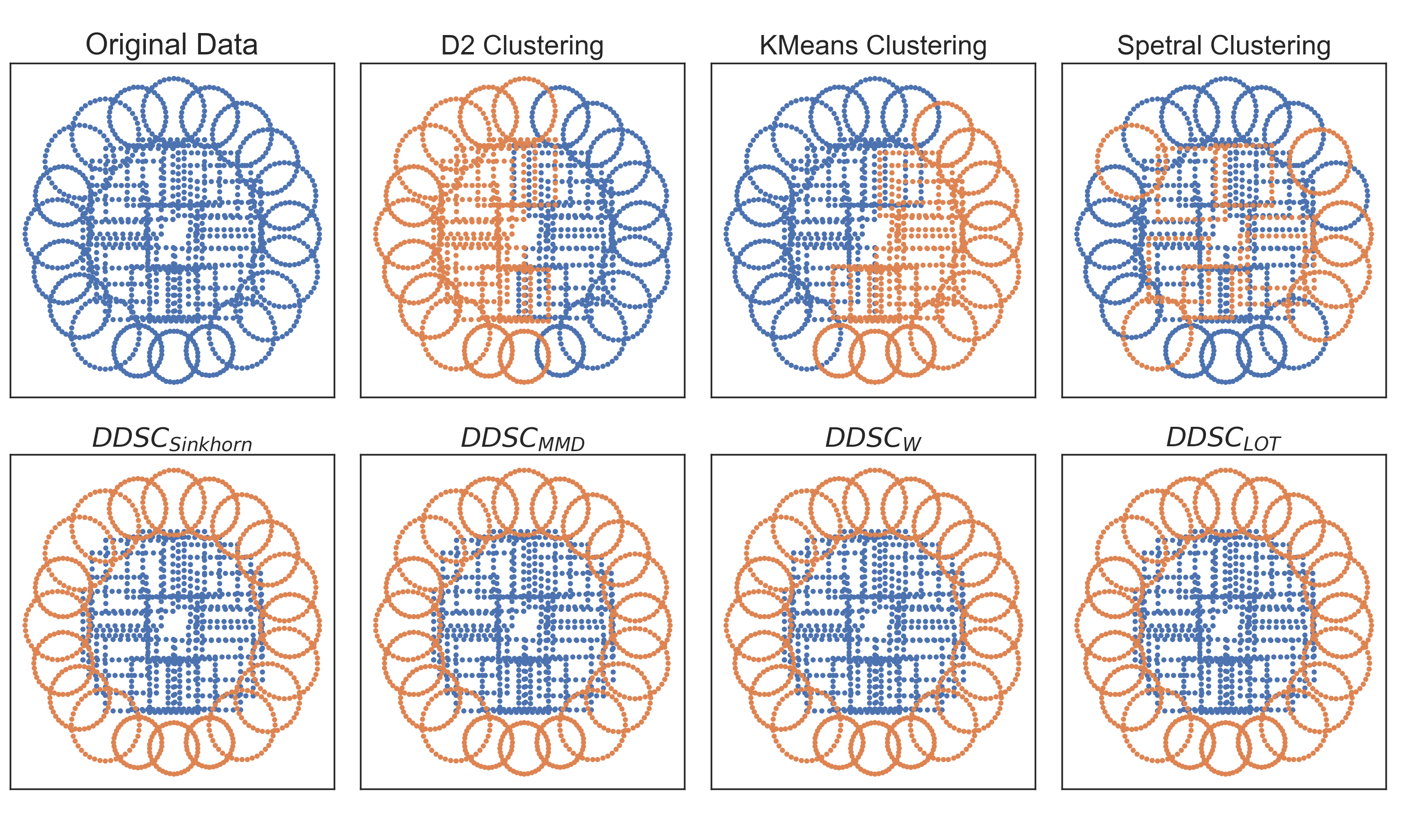
Figure 2. Clustering results of the toy dataset. Different colors indicate different clusters generated from the algorithm. There are 20 square-shaped and circle-shaped distributions, respectively. Each distribution has 40 support points in $\mathbb{R}^{2}$ space.

Table 1. AMI scores for toy example clustering results

baseline	K-means	SC	D2
AMI	0.0	0.0	0.0
proposed	DDSC${}_{\text{Sinkhorn}}$	DDSC${}_{\text{MMD}}$	DDSC${}_{\text{W}}$	DDSC${}_{\text{LOT}}$
AMI	1.0	1.0	1.0	1.0

5.2. Real Dataset

The idea of treating each document as a bag of words has been explored in previous works. In our experiments, we use three widely used text datasets to evaluate our methods. BBCnews abstract dataset: Concatenate the title and the first sentence of news posts from BBCNews dataset, which is the same construction as (Ye et al., 2017a). Domain-specific dataset BBCSports abstract is constructed similarly as the BBCNews abstract. The “Reuters subset” is a 5-class subset of the Reuters dataset. To ensure completeness, we also explore two image datasets. We take a subset of 1000 images (100 images for each class) from the well-know MNIST (Deng, 2012) and Fashion-MNIST (Xiao et al., 2017) dataset. More information are shown in Table 2.

Table 2. Description of real text dataset used in our experiments. $N$ is the number of distributions. $n$ is the number of samples in each distribution. $d$ is the dimension of data. $K$ is the number of clusters of the true labels.

Dataset	$N$	$d$	$n$	$K$
BBCSports abstr.	737	300	16	5
BBCNews abstr.	2,225	300	16	5
Reuters	1,209	300	16	5
MNIST	1,000	2	784	10
Fashion-MNIST	1,000	2	784	10

Table 3. Clustering results (average over five runs) of the real text datasets. * indicates the result is a reference from the work of Huang et al. (2021). The bold figures are the best 4 results.

	BBC-Sports abstr.		BBCNew abstr.		Reuters Subsets		Average Score
Methods	AMI	ARI	AMI	ARI	AMI	ARI	AMI	ARI
K-means	0.3408	0.3213	0.5328	0.4950	0.4783	0.4287	0.4506	0.4150
K-means∗	0.4276	-	0.3877	-	0.4627	-	0.4260	-
SC	0.3646	0.2749	0.4891	0.4659	0.3955	0.3265	0.4164	0.3558
D2	0.6234	0.4665	0.6111	0.5572	0.4244	0.3966	0.5530	0.4734
D2∗	0.6510	-	0.6095	-	0.4200	-	0.5602	-
PD2	0.6300	0.4680	0.6822	0.6736	0.4958	0.3909	0.6027	0.5108
PD2∗	0.6892	-	0.6557	-	0.4713	-	0.6054	-
DDSC${}_{\text{MMD}}$	0.6724	0.5399	0.7108	0.6479	0.5803	0.5105	0.6545	0.5661
DDSC${}_{\text{Sinkhorn}}$	0.7855	0.7514	0.7579	0.7642	0.6096	0.5457	0.7177	0.6871
DDSC${}_{\text{W}}$	0.7755	0.7424	0.7549	0.7585	0.6096	0.5457	0.7133	0.6802
DDSC${}_{\text{LOT}}$	0.7150	0.6712	0.7265	0.7499	0.5290	0.4325	0.6580	0.6129

We compare our DDSC${}_{\text{MMD}}$, DDSC${}_{\text{Sinkhorn}}$, DDSC${}_{\text{W}}$, and DDSC${}_{\text{LOT}}$ models with the following four baselines: (1) Spectral Clustering (SC) (2) K-means Clustering (K-means) (3) D2 Clustering (D2) (4) PD2 clustering (PD2). D2 clustering is proposed in Ye et al. (2017b) as described in Section 2.4. PD2 clustering Huang et al. (2021) projects the original support points into a lower dimension first and then apply D2 clustering. We don’t apply PD2 clustering on image datasets because image data only have 2 dimensions. For all the methods, we tested the number of clusters $K\in\{5,6,7,8,9,10\}$. For DDSC${}_{\text{Sinkhorn}}$, we choose the Sinkhorn regularizer $\varepsilon$ between $1$ and $10$. Only the best results are reported.

The results of the numerical experiment of text datasets and image datasets are shown in Table 3 and Table 4 respectively. We also include experiment results of (Huang et al., 2021) which use the same text data and preprocessing as our experiment. Our methods outperform barycenter-based clustering (e.g. D2 Clustering) and other baselines a lot for both text datasets and image datasets.

Table 4. Clustering results (average over five runs) of the image datasets (subsets).

	MNIST		Fashion-MNIST
Methods	AMI	ARI	AMI	ARI
K-means	0.5074	0.3779	0.5557	0.4137
SC	0.4497	0.3252	0.5135	0.3175
D2	0.3649	0.2172	0.5693	0.4174
DDSC${}_{\text{MMD}}$	0.7755	0.6742	0.6553	0.4912
DDSC${}_{\text{Sinkhorn}}$	0.6974	0.6150	0.6332	0.4346
DDSC${}_{\text{W}}$	0.7073	0.6199	0.6292	0.4691
DDSC${}_{\text{LOT}}$	0.6754	0.4992	0.6309	0.4469

We explored the scalability of our methods. In this section, we study both the time complexity and empirical running time of D2, DDSC${}_{\text{MMD}}$, DDSC${}_{\text{Sinkhorn}}$, DDSC${}_{\text{LOT}}$, DDSC${}_{\text{W}}$. We don’t include the running time of PD2 because of the highly time-consuming projection process. Suppose there are $N$ distributions, and each distribution has $m$ support points. First, we point out the time complexity of different methods in Table 5. We also report the average running time of 5 experiments in Table 6.

Table 5. Time complexity of different methods. Assume the number of iterations for Sinkhorn divergences, barycenter is $T_{1}$, $T_{2}$ respectively.

Model	Time Complexity
D2	$O(T_{2}Nm^{2}+NKm^{3}\log{m})$
DDSC${}_{\text{MMD}}$	$O(N^{2}m^{2}+N^{3})$
DDSC${}_{\text{Sinkhorn}}$	$O(T_{1}N^{2}m^{2}+N^{3})$
DDSC${}_{\text{W}}$	$O(N^{2}m^{3}\log{m}+N^{3})$
DDSC${}_{\text{LOT}}$	$O(Nm^{3}\log{m}+N^{3})$

Table 6. Running time (seconds) of different methods.

	BBC-S	BBC-N	Reuters	MNIST	F-MNIST
D2	99.3	640.2	305.7	910.5	2250.0
DDSC${}_{\text{MMD}}$	24.5	200.8	80.4	376.1	364.0
DDSC${}_{\text{Sinkhorn}}$	86.0	1252.7	755.9	845.9	3075.4
DDSC${}_{\text{W}}$	44.9	427.7	139.9	1545.5	10595.1
DDSC${}_{\text{LOT}}$	12.1	73.8	38.2	251.2	251.0

In terms of running time, DDSC${}_{\text{MMD}}$ outperforms the D2 Clustering because solving Wasserstein barycenter in D2 clustering is based on an iterative method while MMD distance has a closed-form solution. DDSC${}_{\text{W}}$ requires less time than DDSC${}_{\text{Sinkhorn}}$ for text datasets while we get an opposite result on image datasets. This is because the number of support points $m$ in text datasets is relatively small. The advantage of Sinkhorn divergences over Wasserstein distance is not obvious because it may need lots of iterations to converge. The cost of calculating Wasserstein distances on data (e.g. images) with a large number of support points (large $m$) is very large. DDSC${}_{\text{Sinkhorn}}$ will be more suitable if the number of support points is large. DDSC${}_{\text{LOT}}$ performs best in terms of running time.

6. Conclusion

This work proposed a general framework for discrete distribution clustering based on spectral clustering. Using this framework in practice for discrete distribution clustering has two reasons: distributions in real scenarios may not concentrate at some centroids but lie in some irregular shapes or on multiple manifolds; we may not want to solve the barycenter problem that requires careful initialization and has a high computational cost. Both issues can be solved by our framework. To improve the scalability of our methods, we proposed a linear optimal transport based method under the framework. We also provided theoretical analysis for consistency and correctness of clustering. Numerical results on synthetic datasets, real text, and image datasets showed that our methods outperformed the baseline methods largely, in terms of both clustering accuracy and clustering efficiency.

Appendix A Proof for similarity matrix Error bound

We first propose the following error bound of the similarity matrix.

Lemma A.1 (Error bound of similarity matrix).

With probability at least $1-N\tau\theta$, the estimated similarity matrix $\mathbf{\hat{A}}$ satisfies

(22) $$\|\mathbf{A}-\mathbf{\hat{A}}\|_{\infty}<\sqrt{\gamma}\rho+E\sqrt{\gamma\log{\frac{1}{\theta}}},$$

where $\rho$ and $E$ are defined as before in Lemma 4.1 and $\gamma$ was defined in Eq (11).

Proof.

To analyze $\|\mathbf{A}-\hat{\mathbf{A}}\|_{\infty}$, we first look at a single element in $\mathbf{A}-\hat{\mathbf{A}}$,

(23) $$|a_{ij}-\hat{a}_{ij}|=|\exp(-\gamma D_{ij}^{2})-\exp(-\gamma\hat{D}_{ij}^{2})|$$

Since $|e^{-x^{2}}-e^{-y^{2}}|<|x-y|$ for $x,y>0$,

(24) $$|a_{ij}-\hat{a}_{ij}|<\gamma^{1/2}|D_{ij}-\hat{D}_{ij}|$$

Let $\zeta=\sqrt{\gamma}\rho+E\sqrt{\gamma\log{\frac{1}{\theta}}}$. According to Lemma 4.1, with probability at least $1-\theta$

(25) $$|a_{ij}-\hat{a}_{ij}|<\zeta$$

Since we only keep $N\tau$ elements in $\hat{\mathbf{A}}$, we use $N\tau$ random variables $X_{i},i=1,\dots,N\tau$ to denote the elements in $|\mathbf{A}-\hat{\mathbf{A}}|$. We now want to find the probability that the largest element in $|\mathbf{A}-\hat{\mathbf{A}}|$ smaller than $\zeta$ By Boole’s inequality,

(26) $$\mathcal{P}\left(\bigcup_{i=1}^{N\tau}(X_{i}\geq\zeta)\right)\leq\sum_{i=1}^{N\tau}\mathcal{P}\left(X_{i}\geq\zeta\right)$$

From equation( 25) we know that $\mathcal{P}(X_{i}<\zeta)\geq 1-\theta$, so $\mathcal{P}(X_{i}\geq\zeta)<\theta$. Combine with equation( 26), we have

(27) $$\mathcal{P}\left(\bigcup_{i=1}^{N\tau}(X_{i}\geq\zeta)\right)<N\tau\theta$$

We can derive the error bound as follows,

(28) $$\mathcal{P}\left(\|\mathbf{A}-\hat{\mathbf{A}}\|_{\infty}<\zeta\right) =\mathcal{P}\left(\max\{X_{i}\}_{i=1}^{N\tau}<\zeta\right)$$

$$=\mathcal{P}\left(X_{1}<\zeta,\dots,X_{N\tau}<\zeta\right)$$

$$=1-\mathcal{P}\left(\bigcup_{i=1}^{N\tau}(X_{i}\geq\zeta)\right)$$

$$\geq 1-N\tau\theta$$

So the error bound for similarity is

(29) $$\|\mathbf{A}-\hat{\mathbf{A}}\|_{\infty}<\zeta$$

with probability at least $1-N\tau\theta$. ∎

Appendix B Proof for Laplacian matrix Error Bound

Let $\mathbf{L}$ and $\mathbf{\hat{L}}$ be the Laplacian matrices of $\mathbf{A}$ and $\mathbf{\hat{A}}$ respectively. We provide the estimation error bound for $\mathbf{\hat{L}}$ in the following lemma.

Lemma B.1 (Error bound of Laplacian matrix).

Suppose the minimum value of the adjacency matrix $\mathbf{A}$ is $\alpha$. Then with probability at least $1-2\tau^{2}N\theta$, the following inequality holds $\mathbf{\hat{L}}$ satisfies

(30) $$\|\mathbf{L}-\mathbf{\hat{L}}\|_{\infty}<\frac{2\zeta}{\tau(\alpha-\zeta)^{2}},$$

where $\zeta=\sqrt{\gamma}\rho+E\sqrt{\gamma\log{\frac{1}{\theta}}}$.

Proof.

By definition, $\mathbf{L}=\mathbf{I}-\mathbf{S}^{-1/2}\mathbf{A}\mathbf{S}^{-1/2}$, $\hat{\mathbf{L}}=\mathbf{I}-\hat{\mathbf{S}}^{-1/2}\hat{\mathbf{A}}\hat{\mathbf{S}}^{-1/2}$. We have

(31) $$\|\mathbf{L}-\hat{\mathbf{L}}\|_{\infty}=\|\mathbf{S}^{-1/2}\mathbf{A}\mathbf{S}^{-1/2}-\hat{\mathbf{S}}^{-1/2}\hat{\mathbf{A}}\hat{\mathbf{S}}^{-1/2}\|_{\infty}$$

For $ij$-th entry of matrix $\hat{\mathbf{L}}-\mathbf{L}$,

(32) $$(\mathbf{L}-\hat{\mathbf{L}})_{ij}=\frac{a_{ij}}{\sqrt{s_{i}}\sqrt{s_{j}}}-\frac{\hat{a}_{ij}}{\sqrt{\hat{s}_{i}}\sqrt{\hat{s}_{j}}}$$

Consider a single element in $\hat{\mathbf{L}}-\mathbf{L}$,

(33) $$\left|\frac{a_{ij}}{\sqrt{s_{i}}\sqrt{s_{j}}}-\frac{\hat{a}_{ij}}{\sqrt{\hat{s}_{i}}\sqrt{\hat{s}_{j}}}\right|$$

$$= \Big{|}\frac{a_{ij}}{\sqrt{s_{i}}\sqrt{s_{j}}}-\frac{a_{ij}}{\sqrt{\hat{s}_{i}}\sqrt{s_{j}}}+\frac{a_{ij}}{\sqrt{\hat{s}_{i}}\sqrt{s_{j}}}-\frac{\hat{a}_{ij}}{\sqrt{\hat{s}_{i}}\sqrt{s_{j}}}$$

$$+\frac{\hat{a}_{ij}}{\sqrt{\hat{s}_{i}}\sqrt{s_{j}}}-\frac{\hat{a}_{ij}}{\sqrt{\hat{s}_{i}}\sqrt{\hat{s}_{j}}}\Big{|}$$

$$\leq \left|\frac{1}{\sqrt{s_{i}}}-\frac{1}{\sqrt{\hat{s}_{i}}}\right|\frac{a_{ij}}{\sqrt{s_{j}}}+\left|a_{ij}-\hat{a}_{ij}\right|\frac{1}{\sqrt{\hat{s}_{i}}\sqrt{s_{j}}}$$

$$+\left|\frac{1}{\sqrt{s_{j}}}-\frac{1}{\sqrt{\hat{s}_{j}}}\right|\frac{a_{ij}}{\sqrt{\hat{s}_{i}}}$$

Let $f(x):=\frac{1}{\sqrt{x}}$. By Mean Value Theorem,

(34) $$f(s_{i})-f(\hat{s}_{i})=\frac{df}{dx}(c)(s_{i}-\hat{s}_{i})$$

for some value $c$ between $s_{i}$ and $\hat{s}_{i}$. That is,

(35) $$\left|\frac{1}{\sqrt{s_{i}}}-\frac{1}{\sqrt{\hat{s}_{i}}}\right| \leq\frac{1}{2c^{\frac{3}{2}}}\left|s_{i}-\hat{s}_{i}\right|$$

From Lemma A.1 we know that $\left|a_{ij}-\hat{a}_{ij}\right|<\zeta$ with probability at least $(1-\theta)$. Since we only keep $\tau$ elements in $\mathbf{A}$ and $\hat{\mathbf{A}}$ after sparsing the matrices, by Boole’s inequality, $\left|s_{i}-\hat{s}_{i}\right|<\tau\zeta$ with probability at least $(1-\tau\theta)$. The minimum value of $\mathbf{A}$ is $\alpha$,then by Lemma A.1, the minimum possible value of $\hat{\mathbf{A}}$ is $(\alpha-\zeta)$. Notice that in practice we can always assume $\alpha>\zeta$ because the minimum entry of $\hat{\mathbf{A}}$ will never be negative. Therefore, the minimum value of $s_{i}$ is $\tau\alpha$ and the minimum value of $\hat{s}_{i}$ is $\tau(\alpha-\zeta)$. Since $c$ is a value between $s_{i}$ and $\hat{s}_{i}$, the minimum value of $c$ is $\tau(\alpha-\zeta)$. Then we have

(36) $$\left|\frac{1}{\sqrt{s_{i}}}-\frac{1}{\sqrt{\hat{s}_{i}}}\right|\frac{a_{ij}}{\sqrt{s_{j}}} <\frac{\tau\zeta}{2(\tau(\alpha-\zeta))^{\frac{3}{2}}}\frac{a_{ij}}{\sqrt{s_{j}}}$$

$$\leq\frac{\tau\zeta}{2(\tau(\alpha-\zeta))^{\frac{3}{2}}}\frac{1}{\sqrt{s_{j}}}$$

$$\leq\frac{\tau\zeta}{2(\tau(\alpha-\zeta))^{\frac{3}{2}}}\frac{1}{\sqrt{\tau\alpha}}$$

$$\leq\frac{\tau\zeta}{2(\tau(\alpha-\zeta))^{\frac{3}{2}}}\frac{1}{\sqrt{\tau(\alpha-\zeta)}}$$

$$=\frac{\zeta}{2\tau(\alpha-\zeta)^{2}}$$

with probability at least $(1-\tau\theta)$. Also, it is easy to see that with probability at least $(1-\tau\theta)$,

(37) $$\left|a_{ij}-\hat{a}_{ij}\right|\frac{1}{\sqrt{\hat{s}_{i}}\sqrt{s_{j}}} <\frac{\zeta}{\sqrt{\hat{s}_{i}}\sqrt{s_{j}}}$$

$$\leq\frac{\zeta}{\tau\sqrt{\alpha-\zeta}\sqrt{\alpha}}$$

$$\leq\frac{\zeta}{\tau(\alpha-\zeta)}$$

With similar steps as inequalities 36, we can derive that with probability at least $(1-\tau\theta)$

(38) $$\left|\frac{1}{\sqrt{s_{j}}}-\frac{1}{\sqrt{\hat{s}_{j}}}\right|\frac{a_{ij}}{\sqrt{\hat{s}_{i}}}<\frac{\zeta}{2\tau(\alpha-\zeta)^{2}}$$

Combining equations 36, 37 and 38, we have

(39) $$\left|\frac{a_{ij}}{\sqrt{s_{i}}\sqrt{s_{j}}}-\frac{\hat{a}_{ij}}{\sqrt{\hat{s}_{i}}\sqrt{\hat{s}_{j}}}\right|$$

$$< \frac{\zeta}{2\tau(\alpha-\zeta)^{2}}+\frac{\zeta}{\tau(\alpha-\zeta)}+\frac{\zeta}{2\tau(\alpha-\zeta)^{2}}$$

$$= \frac{\zeta}{\tau}\cdot\frac{1+\alpha-\zeta}{(\alpha-\zeta)^{2}}$$

$$\leq \frac{2\zeta}{\tau(\alpha-\zeta)^{2}}$$

with probability at least $(1-2\tau\theta)$. Using Boole’s inequality and similar arguments in Appendix A, we have

(40) $$\|\mathbf{L}-\hat{\mathbf{L}}\|_{\infty}\leq\frac{2\zeta}{\tau(\alpha-\zeta)^{2}}$$

with probability at least $(1-2\tau^{2}N\theta)$. ∎

Appendix C Proof for Theorem 4.3

We use the famous Davis-Kahan theorem from matrix perturbation theory to find the bound. The following lemma bounds the difference between eigenspaces of symmetric matrices under perturbations.

Lemma C.1 (Davis-Kahan Theorem).

Let $\mathbf{Z},\mathbf{H}\in\mathbb{R}^{n\times n}$ be any symmetric matrices. Consider $\hat{\mathbf{Z}}:=\mathbf{Z}+\mathbf{H}$ as a pertued version of $\mathbf{Z}$. Let $S_{1}\subset\mathbb{R}$ be an interval. Denote by $\lambda_{S_{1}}(\mathbf{Z})$ the set of eigenvalues of $\mathbf{Z}$ which are contained in $S_{1}$, and by $\mathbf{V}_{1}$ the eigenspace corresponding to all those eigenvalues. Denote by $\lambda_{S_{1}}(\hat{\mathbf{Z}})$ and $\hat{\mathbf{V}}_{1}$ the analogous quantities for $\hat{\mathbf{Z}}$. Define the distance between $S_{1}$ and the spectrum of $\mathbf{Z}$ outside of $S_{1}$ as

$$\delta=\min\{|\lambda-s|;\lambda\in eig(\mathbf{Z}),\lambda\notin S_{1},s\in S_{1}\}.$$

Then the distance between the two subspaces $\mathbf{V}_{1}$ and $\hat{\mathbf{V}}_{1}$ is bounded by

$$d(\mathbf{V}_{1},\hat{\mathbf{V}}_{1})\leq\frac{\|\mathbf{H}\|_{F}}{\delta}.$$

Following Lemma C.1, in our case, $\delta=|\lambda_{K+1}-\lambda_{K}|$ is the eigen-gap of Laplacian $\mathbf{L}$ and $\mathbf{H}=\hat{\mathbf{L}}-\mathbf{L}$ is the perturbation. To ensure $\xi$-consistency, we only need

(41) $$\frac{\|\mathbf{L}-\hat{\mathbf{L}}\|_{F}}{\delta}\leq\xi.$$

According to Appendix B, an arbitrary element in $|\mathbf{L}-\hat{\mathbf{L}}|$ is less than $\frac{2\zeta}{\tau(\alpha-\zeta)^{2}}$ with probability at least $1-2\tau\theta$. So we have

(42) $$\|\mathbf{L}-\hat{\mathbf{L}}\|_{F} <\sqrt{N\tau}\cdot\frac{2\zeta}{\tau(\alpha-\zeta)^{2}}$$

$$=\frac{2\zeta\sqrt{N}}{(\alpha-\zeta)^{2}\sqrt{\tau}}$$

with probability at least $1-2\tau^{2}N\theta$.

So a sufficient condition for $\xi$-consistent clustering as defined in Definition 4.2 is

(43) $$\frac{2\zeta\sqrt{N}}{\delta(\alpha-\zeta)^{2}\sqrt{\tau}}<\xi.$$

Appendix D Proof for Theorem 4.7

Consider a distribution $\mu_{i}$, denote $A_{iu}=\max_{k}(\mathbf{A}_{ik}^{inter})$ and $A_{iv}=\min_{k}(\mathbf{A}_{ik}^{intra})$. By assumption, for an arbitrary distributions $\mu_{j}\in\mathcal{N}^{intra}_{i}$ and $\mu_{j\prime}\in\mathcal{N}^{inter}_{i}$,

(44) $$A_{ij}-A_{iu} \geq\xi$$

$$A_{iv}-A_{ij\prime} \geq\xi$$

To ensure correct clustering of DDSC${}_{\text{Sinkhorn}}$, we need to ensure

(45) $$\hat{A}_{ij} \geq\hat{A}_{iu}$$

$$\hat{A}_{ij\prime} \leq\hat{A}_{iv}$$

By proof in Appendix A, we have

(46) $$\left|A_{pq}-\hat{A}_{pq}\right|<\zeta$$

with probability at least $1-\theta$ for arbitrary $p,q$. Therefore, to ensure correct clustering, we only need

(47) $$A_{ij}-\zeta \geq A_{iu}+\zeta$$

$$A_{ij\prime}+\zeta \leq A_{iv}-\zeta$$

Combining inequality 44 and inequality 47, we have

(48) $$\zeta\leq\frac{1}{2}\xi$$

Since we need to satisfy the inequality (46) for $\mu_{j}$ in the connected component $\tau\text{-NN}_{\text{dist}}(\mu_{i})$, so the probability is $1-\tau\theta$. Since there are $N\tau$ distributions to consider in total, the probability is $1-N\tau^{2}\theta$.

Appendix E Robustness Against Noise

We also explore the robustness of different distance matrices against noise. We construct a distance matrix using 2-Wasserstein distance, linear optimal transport distance, MMD distance and Sinkhorn divergences with regularizers $\varepsilon\in\{5,10,50,100,500\}$. Gaussian noise $\mathcal{N}(0,\sigma^{2}I)$ is added to each datapoint. The relative error under noise level $\sigma$ is defined as

$$\text{Relative Error}=med\left(\tfrac{D_{\sigma}-D_{0}}{D_{0}}\right)$$

where $D_{\sigma}$ is the MMD/Sinkhorn distances of the noisy data, $D_{0}$ is the ground truth MMD/Sinkhorn distances of the original data and $\text{med}()$ is the median operator. We use the median value instead of the mean value to mitigate the effect of potential numerical errors in the calculated distance matrix due to the added noise. We set the noise $\sigma\in[0,3.0]$. We set the MMD Gaussian kernel standard deviation to 1. The results are shown in Figure 3.

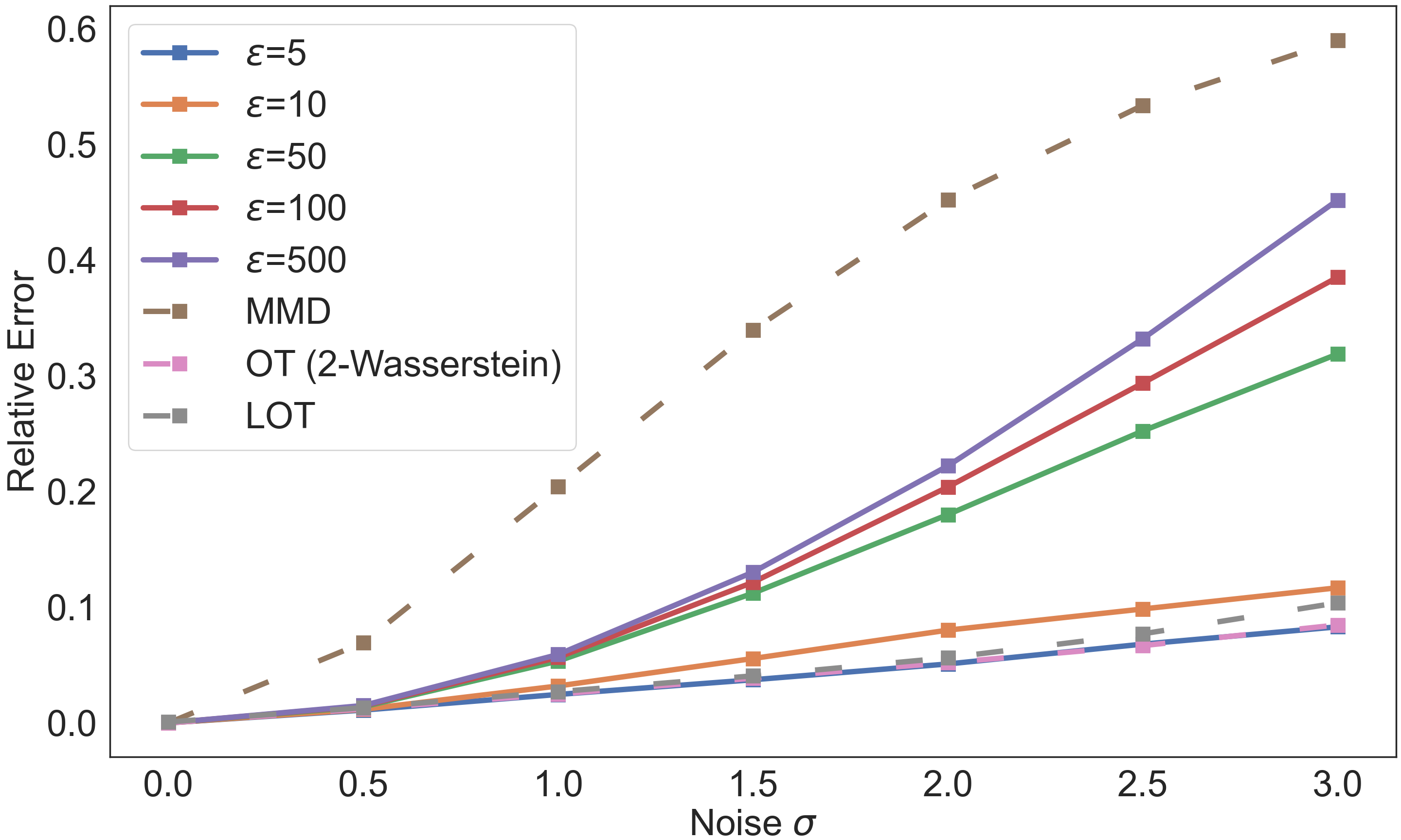
Figure 3. Relative error of distance matrices constructed with different metrics.

From Figure 3, we can see that MMD distance have highest relative error under all noise level. The Sinkhorn divergences with smaller regularizer $\varepsilon$ are more robust against noise. Notice that Sinkhorn divergences interpolate, depending on regularization strength $\varepsilon$, between OT ($\varepsilon=0$) and MMD ($\varepsilon=+\infty$). So we conjecture that the larger the $\varepsilon$, the less robust the distance matrix against noise.

Appendix F Preprocessing of real datasets

We use the pre-trained word-vector dataset GloVe 300d (Pennington et al., 2014) to transform a bag of words into a measure in $\mathbb{R}^{300}$. The TF-IDF scheme normalizes the weight of each word. Before transforming words into vectors, we lower the capital letters, remove all punctuations and stop words and lemmatize each document. We also restrict the number of support points by recursively merging the closest words Huang et al. (2021). For image datasets, images are treated as normalized histograms over the pixel locations covered by the digits, where the support vector is the 2D coordinate of a pixel and the weight corresponds to pixel intensity.

References

- (1)
- Agueh and Carlier (2011) Martial Agueh and Guillaume Carlier. 2011. Barycenters in the Wasserstein Space. SIAM Journal on Mathematical Analysis 43, 2 (2011), 904–924.
- Anderes et al. (2016) Ethan Anderes, Steffen Borgwardt, and Jacob Miller. 2016. Discrete Wasserstein barycenters: Optimal transport for discrete data. Mathematical Methods of Operations Research 84 (2016), 389–409.
- Benamou et al. (2015) Jean-David Benamou, Guillaume Carlier, Marco Cuturi, Luca Nenna, and Gabriel Peyré. 2015. Iterative Bregman projections for regularized transportation problems. SIAM Journal on Scientific Computing 37, 2 (2015), A1111–A1138.
- Cai et al. (2022) Jinyu Cai, Jicong Fan, Wenzhong Guo, Shiping Wang, Yunhe Zhang, and Zhao Zhang. 2022. Efficient deep embedded subspace clustering. In Proceedings of the IEEE/CVF Conference on Computer Vision and Pattern Recognition. 1–10.
- Campello et al. (2015) Ricardo J. G. B. Campello, Davoud Moulavi, Arthur Zimek, and Jörg Sander. 2015. Hierarchical Density Estimates for Data Clustering, Visualization, and Outlier Detection. ACM Trans. Knowl. Discov. Data 10, 1, Article 5 (jul 2015), 51 pages. https://doi.org/10.1145/2733381
- Cuturi (2013) Marco Cuturi. 2013. Sinkhorn Distances: Lightspeed Computation of Optimal Transport. In Advances in Neural Information Processing Systems, C.J. Burges, L. Bottou, M. Welling, Z. Ghahramani, and K.Q. Weinberger (Eds.), Vol. 26. Curran Associates, Inc. https://proceedings.neurips.cc/paper_files/paper/2013/file/af21d0c97db2e27e13572cbf59eb343d-Paper.pdf
- Deng (2012) Li Deng. 2012. The mnist database of handwritten digit images for machine learning research. IEEE Signal Processing Magazine 29, 6 (2012), 141–142.
- Elhamifar and Vidal (2013) E. Elhamifar and R. Vidal. 2013. Sparse Subspace Clustering: Algorithm, Theory, and Applications. IEEE Transactions on Pattern Analysis and Machine Intelligence 35, 11 (2013), 2765–2781.
- Fan (2021) Jicong Fan. 2021. Large-Scale Subspace Clustering via k-Factorization. In Proceedings of the 27th ACM SIGKDD Conference on Knowledge Discovery & Data Mining (Virtual Event, Singapore) (KDD ’21). Association for Computing Machinery, New York, NY, USA, 342–352. https://doi.org/10.1145/3447548.3467267
- Fan et al. (2022) Jicong Fan, Yiheng Tu, Zhao Zhang, Mingbo Zhao, and Haijun Zhang. 2022. A Simple Approach to Automated Spectral Clustering. In Advances in Neural Information Processing Systems, S. Koyejo, S. Mohamed, A. Agarwal, D. Belgrave, K. Cho, and A. Oh (Eds.), Vol. 35. Curran Associates, Inc., 9907–9921.
- Genevay et al. (2019) Aude Genevay, Lénaïc Chizat, Francis Bach, Marco Cuturi, and Gabriel Peyré. 2019. Sample Complexity of Sinkhorn Divergences. In Proceedings of the Twenty-Second International Conference on Artificial Intelligence and Statistics (Proceedings of Machine Learning Research, Vol. 89), Kamalika Chaudhuri and Masashi Sugiyama (Eds.). PMLR, 1574–1583. https://proceedings.mlr.press/v89/genevay19a.html
- Genevay et al. (2016) Aude Genevay, Marco Cuturi, Gabriel Peyré, and Francis Bach. 2016. Stochastic Optimization for Large-scale Optimal Transport. In Advances in Neural Information Processing Systems, D. Lee, M. Sugiyama, U. Luxburg, I. Guyon, and R. Garnett (Eds.), Vol. 29. Curran Associates, Inc. https://proceedings.neurips.cc/paper_files/paper/2016/file/2a27b8144ac02f67687f76782a3b5d8f-Paper.pdf
- Genevay et al. (2018) Aude Genevay, Gabriel Peyre, and Marco Cuturi. 2018. Learning Generative Models with Sinkhorn Divergences. In Proceedings of the Twenty-First International Conference on Artificial Intelligence and Statistics (Proceedings of Machine Learning Research, Vol. 84), Amos Storkey and Fernando Perez-Cruz (Eds.). PMLR, 1608–1617. https://proceedings.mlr.press/v84/genevay18a.html
- Gretton et al. (2006) Arthur Gretton, Karsten Borgwardt, Malte Rasch, Bernhard Schölkopf, and Alex Smola. 2006. A Kernel Method for the Two-Sample-Problem. In Advances in Neural Information Processing Systems, B. Schölkopf, J. Platt, and T. Hoffman (Eds.), Vol. 19. MIT Press. https://proceedings.neurips.cc/paper_files/paper/2006/file/e9fb2eda3d9c55a0d89c98d6c54b5b3e-Paper.pdf
- Gretton et al. (2012) Arthur Gretton, Karsten M Borgwardt, Malte J Rasch, Bernhard Schölkopf, and Alexander Smola. 2012. A kernel two-sample test. The Journal of Machine Learning Research 13, 1 (2012), 723–773.
- Huang et al. (2021) Minhui Huang, Shiqian Ma, and Lifeng Lai. 2021. Projection Robust Wasserstein Barycenters. In Proceedings of the 38th International Conference on Machine Learning (Proceedings of Machine Learning Research, Vol. 139), Marina Meila and Tong Zhang (Eds.). PMLR, 4456–4465.
- Jain et al. (1999) A. K. Jain, M. N. Murty, and P. J. Flynn. 1999. Data Clustering: A Review. ACM Comput. Surv. 31, 3 (sep 1999), 264–323. https://doi.org/10.1145/331499.331504
- Kantorovich (1960) Leonid V Kantorovich. 1960. Mathematical methods of organizing and planning production. Management science 6, 4 (1960), 366–422.
- Kolouri et al. (2021) Soheil Kolouri, Navid Naderializadeh, Gustavo K. Rohde, and Heiko Hoffmann. 2021. Wasserstein Embedding for Graph Learning. arXiv:2006.09430 [cs.LG]
- Kolouri et al. (2017) Soheil Kolouri, Se Rim Park, Matthew Thorpe, Dejan Slepcev, and Gustavo K Rohde. 2017. Optimal mass transport: Signal processing and machine-learning applications. IEEE signal processing magazine 34, 4 (2017), 43–59.
- Kolouri et al. (2016) Soheil Kolouri, Akif B Tosun, John A Ozolek, and Gustavo K Rohde. 2016. A continuous linear optimal transport approach for pattern analysis in image datasets. Pattern recognition 51 (2016), 453–462.
- Kriegel et al. (2009) Hans-Peter Kriegel, Peer Kröger, and Arthur Zimek. 2009. Clustering High-Dimensional Data: A Survey on Subspace Clustering, Pattern-Based Clustering, and Correlation Clustering. ACM Trans. Knowl. Discov. Data 3, 1, Article 1 (mar 2009), 58 pages. https://doi.org/10.1145/1497577.1497578
- Li and Wang (2008) Jia Li and James Z. Wang. 2008. Real-Time Computerized Annotation of Pictures. IEEE Transactions on Pattern Analysis and Machine Intelligence 30, 6 (June 2008), 985–1002. https://doi.org/10.1109/TPAMI.2007.70847
- Liese and Vajda (2006) Friedrich Liese and Igor Vajda. 2006. On divergences and informations in statistics and information theory. IEEE Transactions on Information Theory 52, 10 (2006), 4394–4412.
- Moosmüller and Cloninger (2023) Caroline Moosmüller and Alexander Cloninger. 2023. Linear optimal transport embedding: provable Wasserstein classification for certain rigid transformations and perturbations. Information and Inference: A Journal of the IMA 12, 1 (2023), 363–389.
- Ng et al. (2001) Andrew Ng, Michael Jordan, and Yair Weiss. 2001. On Spectral Clustering: Analysis and an algorithm. In Advances in Neural Information Processing Systems, T. Dietterich, S. Becker, and Z. Ghahramani (Eds.), Vol. 14. MIT Press. https://proceedings.neurips.cc/paper_files/paper/2001/file/801272ee79cfde7fa5960571fee36b9b-Paper.pdf
- Orlin (1988) James Orlin. 1988. A Faster Strongly Polynomial Minimum Cost Flow Algorithm. In Proceedings of the Twentieth Annual ACM Symposium on Theory of Computing (Chicago, Illinois, USA) (STOC ’88). Association for Computing Machinery, New York, NY, USA, 377–387. https://doi.org/10.1145/62212.62249
- Panaretos and Zemel (2019) Victor M Panaretos and Yoav Zemel. 2019. Statistical aspects of Wasserstein distances. Annual review of statistics and its application 6 (2019), 405–431.
- Pandove et al. (2018) Divya Pandove, Shivan Goel, and Rinkl Rani. 2018. Systematic Review of Clustering High-Dimensional and Large Datasets. ACM Trans. Knowl. Discov. Data 12, 2, Article 16 (jan 2018), 68 pages. https://doi.org/10.1145/3132088
- Parsons et al. (2004) Lance Parsons, Ehtesham Haque, and Huan Liu. 2004. Subspace clustering for high dimensional data: a review. SIGKDD Explor. Newsl. 6, 1 (2004), 90–105.
- Pennington et al. (2014) Jeffrey Pennington, Richard Socher, and Christopher Manning. 2014. GloVe: Global Vectors for Word Representation. In Proceedings of the 2014 Conference on Empirical Methods in Natural Language Processing (EMNLP). Association for Computational Linguistics, Doha, Qatar, 1532–1543. https://doi.org/10.3115/v1/D14-1162
- Shi and Malik (2000) Jianbo Shi and Jitendra Malik. 2000. Normalized cuts and image segmentation. IEEE Transactions on pattern analysis and machine intelligence 22, 8 (2000), 888–905.
- Sun et al. (2023) Yan Sun, Yi Han, and Jicong Fan. 2023. Laplacian-Based Cluster-Contractive t-SNE for High-Dimensional Data Visualization. ACM Trans. Knowl. Discov. Data 18, 1, Article 19 (sep 2023), 22 pages. https://doi.org/10.1145/3612932
- Villani (2008) Cédric Villani. 2008. Optimal transport – Old and new. Vol. 338. Springer, xxii+973. https://doi.org/10.1007/978-3-540-71050-9
- Vinh et al. (2009) Nguyen Xuan Vinh, Julien Epps, and James Bailey. 2009. Information Theoretic Measures for Clusterings Comparison: Is a Correction for Chance Necessary?. In Proceedings of the 26th Annual International Conference on Machine Learning (Montreal, Quebec, Canada) (ICML ’09). Association for Computing Machinery, New York, NY, USA, 1073–1080. https://doi.org/10.1145/1553374.1553511
- Wang et al. (2013) Wei Wang, Dejan Slepčev, Saurav Basu, John A Ozolek, and Gustavo K Rohde. 2013. A linear optimal transportation framework for quantifying and visualizing variations in sets of images. International journal of computer vision 101 (2013), 254–269.
- Xiao et al. (2017) Han Xiao, Kashif Rasul, and Roland Vollgraf. 2017. Fashion-MNIST: a Novel Image Dataset for Benchmarking Machine Learning Algorithms. arXiv:1708.07747 [cs.LG]
- Ye et al. (2017a) Jianbo Ye, Yanran Li, Zhaohui Wu, James Z. Wang, Wenjie Li, and Jia Li. 2017a. Determining Gains Acquired from Word Embedding Quantitatively Using Discrete Distribution Clustering. In Proceedings of the 55th Annual Meeting of the Association for Computational Linguistics (Volume 1: Long Papers). Association for Computational Linguistics, Vancouver, Canada, 1847–1856. https://doi.org/10.18653/v1/P17-1169
- Ye et al. (2017b) Jianbo Ye, Panruo Wu, James Z Wang, and Jia Li. 2017b. Fast discrete distribution clustering using Wasserstein barycenter with sparse support. IEEE Transactions on Signal Processing 65, 9 (2017), 2317–2332.
- Zhang et al. (2015) Xianchao Zhang, Xiaotong Zhang, and Han Liu. 2015. Smart Multitask Bregman Clustering and Multitask Kernel Clustering. ACM Trans. Knowl. Discov. Data 10, 1, Article 8 (jul 2015), 29 pages. https://doi.org/10.1145/2747879