A Survey of Deep Learning and Foundation Models for Time Series Forecasting

Abstract.

Deep Learning has been successfully applied to many application domains, yet its advantages have been slow to emerge for time series forecasting. For example, in the well-known Makridakis (M) Competitions, hybrids of traditional statistical or machine learning techniques have only recently become the top performers. With the recent architectural advances in deep learning being applied to time series forecasting (e.g., encoder-decoders with attention, transformers, and graph neural networks), deep learning has begun to show significant advantages. Still, in the area of pandemic prediction, there remain challenges for deep learning models: the time series is not long enough for effective training, unawareness of accumulated scientific knowledge, and interpretability of the model. To this end, the development of foundation models (large deep learning models with extensive pre-training) allows models to understand patterns and acquire knowledge that can be applied to new related problems before extensive training data becomes available. Furthermore, there is a vast amount of knowledge available that deep learning models can tap into, including Knowledge Graphs and Large Language Models fine-tuned with scientific domain knowledge. There is ongoing research examining how to utilize or inject such knowledge into deep learning models. In this survey, several state-of-the-art modeling techniques are reviewed, and suggestions for further work are provided.

1. Introduction

The experience with COVID-19 over the past four years has made it clear to organizations such as the National Science Foundation (NSF) and the Centers for Disease and Prevention (CDC) that we need to be better prepared for the next pandemic. COVID-19 has had huge impacts with 6,727,163 hospitalizations and 1,169,666 deaths as of Saturday, January 13, 2024, in the United States alone (first US case 1/15/2020, first US death 2/29/2020). The next one could be more virulent with greater impacts.

There were some remarkable successes such as the use of messenger RNA vaccines that could be developed much more rapidly than prior approaches. However, the track record for detecting the start of a pandemic and the forecasting of its trajectory leaves room for improvement.

Pandemic Preparedness encapsulates the need for continuous monitoring. Predicting rare events in complex, stochastic systems is very difficult. Transitions from pre-emergence to epidemic to pandemic are easy to see only after the fact. Pandemic prediction using models is critically important as well. Sophisticated models are used to predict the future of hurricanes due to their high impact and potential for loss of life. The impacts of pandemics are likely to be far greater.

As with weather forecasting, accurate pandemic forecasting requires three things: (1) a collection of models, (2) accurate data collection, and (3) data assimilation. If any of these three break down, accuracy drops. When accuracy drops, interventions and control mechanisms cannot be optimally applied, leading to frustration from the public.

During the COVID-19 pandemic data were collected daily, but as seen in Figure 1, there is a very strong weekly pattern that dominates the curve of new deaths that is an artifact of reporting processes. Also, notice how strong hospitalizations and the number of Intensive Care Unit (ICU) patients appear to be good leading indicators.

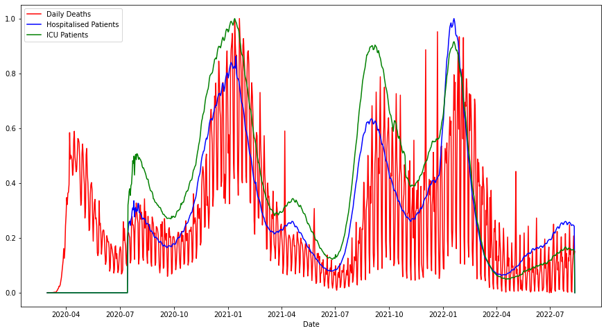
Figure 1. Rescaled Plot of Daily Deaths during the Active Pandemic (note the weekly reporting pattern), Hospitalization, and ICU Patients.

Due to the saw-tooth pattern in the daily deaths, some modeling studies find it better to work off of weekly data. In the later stages of COVID-19, daily reporting stopped, and only weekly remains. Unfortunately, this means that there is much less data available for training deep learning models.

Modeling techniques applied were statistical, machine learning or theory-based compartmental models that were extensions to Susceptible-Infected-Recovered (SIR) or Susceptible-Exposed-Infected-Recovered (SEIR) models. Transitions among these states are governed by differential equations with rate constants that can be estimated from data. Unfortunately, estimating the population of individuals that are in, for example, the exposed state can be very difficult.

The other two categories, statistical and machine learning (including deep learning and foundation models), one could argue are more adaptable to available data as they look for patterns that repeat, dependency on the past, and leading indicators. Both can be formulated as Multivariate Time Series (MTS) forecasting problems, although the related problems of MTS classification and anomaly detection are also very important. Still, having a connection to theory is desirable and could lead to better forecasting in the longer term, as well as a greater understanding of the phenomena. This has led to work in Theory-Guided Data Science (TGDS) (Karpatne et al., 2017; Miller et al., 2017) and Physics-Informed Neural Networks (PINN) (Karniadakis et al., 2021).

Statistical and machine learning techniques complement each other. For example, modeling studies should have reliable baseline models that, from our studies, should include Random Walk (RW), Auto-Regressive (AR), and Seasonal, Auto-Regressive, Integrated, Moving Average with eXogenous variables (SARIMAX). SARIMAX is typically competitive with Deep Learning models when training data are limited. If weekly data are used, the training data will be limited for much of the early stages of the pandemic, just when the need for accurate forecasts is the greatest. Baselines like SARIMAX can also be helpful for hyper-parameter tuning, in that with sufficient data, one would expect deep learning models to perform well; the SARIMAX results can help gauge this. Furthermore, SARIMAX has been used for data augmentation to help train deep learning models (Javeri et al., 2021).

Looking toward the future, this survey paper that extends (Miller et al., 2023) asks the question of how Artificial Intelligence (AI), particularly deep learning, can be used to improve pandemic preparedness and prediction, in terms of better deep learning models, more explainable models, access to scientific literature using Large Language Models (LLM), development and use of knowledge bases and knowledge graphs, as well as better and ongoing assessment of pandemic interventions and controls.

The rest of this paper is organized as follows: Section 2 provides an overview of two waves of improvement in MTS forecasting. Section 3 focuses on recent progress in MTS forecasting looking at Transformers and related modeling techniques. These modeling techniques increasingly strive to better capture temporal dynamics and tend to be the top performers for national-level COVID-19 forecasting. Section 4 focuses on recent progress in MTS forecasting in the spatial-temporal domain, where various types of Graph Neural Networks have a natural appeal. These modeling techniques tend to be applied to state-level COVID-19 data. Foundation models, large pre-trained deep learning models, for time series forecasting are discussed in Section 5. Knowledge in various forms such as Knowledge Graphs is a natural complement to forecasting models, as discussed in Section 6. The knowledge can be used to improve forecasting accuracy, check the reasonableness for forecasts (especially a problem for long-term forecasting), guide the modeling process, and help explain the modeling results. A meta-study comparing the effectiveness of several modeling techniques found in the current literature is given in section 7. Finally, a summary is given in Section 8 that includes looking into a crystal ball to see where MTS might be heading in the future.

2. Progress in MTS Forecasting

The history of time series forecasting dates way back as shown in Table 1. Note that some of the modeling techniques (or model types) have general use other than time series forecasting, but the date and paper reflect their use in forecasting for time series or sequence data. There were, however, periods of rapid progress, for example, the one in the 1950s through the ’70s, and captured in the seminal book by Box and Jenkins (Box and Jenkins, 1970). Another period of substantial progress coincides with the advancement of deep learning, in the 2010s.

Table 1. Types of Time-Series Forecasting Models with Key Initial Reference in Time-Series Context

Model Type	Short Description	Date	Reference
BaselineHA	Historical Average Baseline	.	.
BaselineRW	Random Walk Baseline - guess the previous value	.	.
Regression4TS	Time-Series Regression with Lagged Variables	1949	(Cochrane and Orcutt, 1949)
ARIMA	AutoRegressive, Integrated, Moving-Average	1951	(Whittle, 1951; Box and Jenkins, 1962)
SES	Simple Exponential Smoothing	1957	(Holt Charles, 1957)
VAR	Vector AutoRegressive	1957	(Quenouille and Quenouille, 1957)
VARMA	Vector AutoRegressive, Moving-Average	1957	(Quenouille and Quenouille, 1957)
VECM	Vector Error Correction Model	1957	(Quenouille and Quenouille, 1957)
ES	Exponential Smoothing (Holt-Winters)	1960	(Winters, 1960)
SARIMA	Seasonal ARIMA	1967	(Box et al., 1967)
SARIMAX	SARIMA, with eXogenous variables	1970	(Box and Jenkins, 1970)
NAR/NARX	Nonlinear AutoRegressive, Exogenous	1978	(Jones and Cox, 1978)
Neural Network	Neural Network	1988	(Smith et al., 1988)
RNN	Recurrent Neural Network	1989	(Williams and Zipser, 1989)
FDA/FTSA	Functional Data/Time-Series Analysis	1991	(Ramsay and Dalzell, 1991)
CNN	Convolutional Neural Network	1995	(LeCun et al., 1995)
SVR	Support Vector Regression	1997	(Müller et al., 1997)
LSTM	Long, Short-Term Memory	1997	(Hochreiter and Schmidhuber, 1997)
ELM	Extreme Learning Machine	2007	(Singh and Balasundaram, 2007)
GRU	Gated Recurrent Unit	2014	(Cho et al., 2014)
Encoder-Decoder	Encoder-Decoder with Attention	2014	(Chorowski et al., 2014)
MGU	Minimal Gated Unit	2016	(Zhou et al., 2016)
TCN	Temporal Convolutional Network	2016	(Lea et al., 2016)
GNN/GCN	Graph Neural/Convolutional Network	2016	(Kipf and Welling, 2016)
vTRF	(Vanilla) Transformer	2017	(Vaswani et al., 2017)

There are several open source projects that support time series analysis across programming languages:

• R: Time Series [https://cran.r-project.org/web/views/TimeSeries.html] consists of a large collection of time series models.

• Python: Statsmodels [https://www.statsmodels.org/stable/index.html] provides a basic collection of time series models. Sklearn [https://scikit-learn.org/stable] and a related package, Sktime [https://www.sktime.net/en/stable], provide most of the models offered by Statsmodels. PyTorch-Forecasting [https://github.com/jdb78/pytorch-forecasting?tab=readme-ov-file] includes several types of Recurrent Neural Networks. TSlib [https://github.com/thuml/Time-Series-Library] provides several types of Transformers used for time series analysis.

• Scala: Apache Spark [https://spark.apache.org/] has a limited collection of time series models. ScalaTion [https://cobweb.cs.uga.edu/~jam/scalation.html], [https://github.com/scalation] (Miller et al., 2010) supports most of the modeling techniques listed in Table 1. In addition, it supports several forms of Time-Series Regression, including recursive ARX, direct ARX_MV, quadratic, recursive ARX_Quad, and quadratic, direct ARX_Quad_MV.

Forecasting the future is a very difficult thing to do and until recently, machine learning models did not offer much beyond what statistical models provided, as born out in the M Competitions.

2.1. M Competitions

The Makridakis or M Competitions began in 1982 and have continued with M6 which took place 2022-2023. In the M4 competition ending in May 2018, the purely ML techniques performed poorly, although a hybrid neural network (LSTM) statistical (ES) technique (Smyl, 2020) was the winner (Makridakis et al., 2018). The rest of the top performers were combinations of statistical techniques. Not until the M5 competition ended in June 2020, did Machine Learning (ML) modeling techniques become better than classical statistical techniques. Several top performers included LightGBM in their combinations (Makridakis et al., 2022). LightGBM is a highly efficient implementation of Gradient Boosting Decision/Regression Trees (Ke et al., 2017). Multiple teams included neural networks in their combinations as well. In particular, deep learning techniques such as DeepAR consisting of multiple LSTM units (Salinas et al., 2020) and N-BEATS, consisting of multiple Fully Connected Neural Network blocks (Oreshkin et al., 2019) were applied. Many of them also combined recursive (e.g., uses $t+1$ prior forecast for $t+2$ forecast) and direct (non-recursive) forecasting. “In M4, only two sophisticated methods were found to be more accurate than simple statistical methods, where the latter occupied the top positions in the competition. By contrast, all 50 top-performing methods were based on ML in M5”. (Makridakis et al., 2022) The M6 competition involves both forecasting and investment strategies (Makridakis et al., 2023) with summaries of its results expected in 2024.

2.2. Statistical and Deep Learning Models for Time Series

As illustrated by the discussion of the M Competitions, machine learning techniques took some time to reach the top of the competition. Neural Network models demonstrated highly competitive results in many domains, but less so in the domain of time series forecasting, perhaps because the patterns are more elusive and often changing. Furthermore, until the big data revolution, the datasets were too small to train a neural network having a large number of parameters.

2.2.1. First Wave

From the first wave of progress, SARIMAX models have been shown to generally perform well, as they can use past and forecasted values of the endogenous time series, past errors/shocks for the endogenous time series, and past values of exogenous time series. In addition, differencing of the endogenous variable may be used to improve its stationarity, and furthermore, seasonal/periodic patterns can be utilized. As an aside, many machine learning papers have compared their models to ARIMA, yet SARIMAX is still efficient and is often superior to ARIMA. In addition, the M4 and M5 Competitions indicated that Exponential Smoothing can provide simple and accurate models.

The most straightforward time series model for MTS is a Vector Auto-Regressive (VAR) model with $p$ lags over $n$ variables ${\rm VAR}(p,n)$. For example, a 3-lag, bi-variate VAR(3, 2) model can be useful in pandemic forecasting as new hospitalizations and new deaths are related variables for which time series data are maintained, i.e., $y_{t0}$ is the number of new hospitalizations at time $t$ and $y_{t1}$ is the number of new deaths at time $t$. The model (vector) equation may be written as follows:

(1) $${\bf y}_{t}~{}=~{}{\boldsymbol{\delta}}\,+\,\Phi^{(0)}{\bf y}_{t-1}\,+\,\Phi^{(1)}{\bf y}_{t-2}\,+\,\Phi^{(2)}{\bf y}_{t-3}\,+\,\boldsymbol{\epsilon}_{t}$$

where ${\boldsymbol{\delta}}\in\mathbb{R}^{2}$ is a constant vector, $\Phi^{(0)}\in\mathbb{R}^{2\times 2}$ is the parameter matrix for the first lag, $\Phi^{(1)}\in\mathbb{R}^{2\times 2}$ is the parameter matrix for the second lag, $\Phi^{(2)}\in\mathbb{R}^{2\times 2}$ is the parameter matrix for the third lag, and ${\boldsymbol{\epsilon}_{t}}\in\mathbb{R}^{2}$ is the residual/error/shock vector. Some research has explored VARMA but has found them to be only slightly more accurate than VAR models, but more complex, as they can weigh in past errors/shocks (Athanasopoulos and Vahid, 2008). SARIMAX and VAR can both be considered models for multivariate time series, the difference is that SARIMAX focuses on one principal variable, with the other being used as indicators for those variables, for example, using new_cases and hospitalizations time series to help forecast new_deaths. SARIMAX tends to suffer less from the compounding of errors than VAR. A SARIMAX model can be trimmed down to an ARX model (Auto-Regressive, eXogenous) to see the essential structure of the model consisting of the first $p$ lags of the endogenous variable along with lags $[a,b]$ of the exogenous variable ${\rm ARX}(p,[a,b])$. For example, the model equation for an ARX(3, [2, 3]) may be written as follows:

(2) $$y_{t}~{}=~{}\delta\,+\,\phi_{0}y_{t-1}\,+\,\phi_{1}y_{t-2}\,+\,\phi_{2}y_{t-3}\,+\,\beta_{0}x_{t-2}\,+\,\beta_{1}x_{t-3}\,+\,\epsilon_{t}$$

where $\hat{y}_{t}$, the forecasted value, is the same formula without $\epsilon_{t}$. The MTS in this case consists of one endogenous time series $y_{t}$ and one exogenous time series $x_{t}$ for $t\in 0..m-1$. All the parameters $\delta,\phi_{0},\phi_{1},\phi_{2},\beta_{0}$ and $\beta_{1}$ are now scalars. ARX models may have more than one exogenous times series (see (Pearl, 2011) for a discussion of endogenous vs. exogenous variables). The specification of a SARIMAX model subsumes the ARX specification,

(3) $${\rm SARIMAX}(p,d,q)_{\times}(P,D,Q)_{s}\,[a,b]$$

where $p$ is the number of Auto-Regressive (AR) terms/lagged endogenous values, $d$ is the number of stride-1 differences (Integrations (I)) to take, $q$ is the number of moving average (MA) terms/lagged shocks, $P$ is the number of seasonal (stride-$s$) Auto-Regressive (AR) terms/lagged endogenous values, $D$ is the number of stride-$s$ differences to take, $Q$ is the number of seasonal (stride-$s$) moving average (MA) terms/lagged shocks, $s$ is the seasonal period (e.g., week, month, or whatever time period best captures the pattern) and $[a,b]$ is the range of exogenous (X) lags to include. Again, there may be multiple exogenous variables. Although the optimal values for parameters of ARX models may be found very efficiently by solving a system of linear equations, for example, using matrix factorization, inclusion of the MA terms makes the equation non-linear, so the loss function (e.g., Mean Squared Error (MSE) or Negative Log-Likelihood (NLL)) is usually minimized using a non-linear optimizer such as the Limited-memory Broyden-Fletcher-Goldfarb-Shanno (L-BFGS) algorithm (Liu and Nocedal, 1989).

2.2.2. Second Wave

The story is not complete for the second wave. The M5 Competition showed the value of LightGBM. Studies have shown that LSTM and GRU tend to perform similarly and usually outperform Feedforward Neural Networks (FNN).

The idea of a Recurrent Neural Network (RNN) is to take a weighted combination of an input vector ${\bf x}_{t}$ (recent history) and a hidden state vector (decaying long-term history) and activate it to compute the new state ${\bf h}_{t}$. A final layer converts this to a time series forecast(s) $\hat{y}_{t}$.

$${\bf x}_{t} ~{}=~{}[y_{t-p},\dots,y_{t-1}] {\rm input~{}vector}$$

$${\bf h}_{t} ~{}=~{}{\bf f}(U{\bf x}_{t}+W{\bf h}_{t-1}\,+\,{\boldsymbol{\beta}^{(h)}}) {\rm hidden~{}state~{}vector}$$

$$\hat{y}_{t} ~{}=~{}g(V{\bf h}_{t}\,+\,\beta^{(y)}) {\rm output~{}scalar}$$

where $U$, $W$, and $V$ are learnable weight matrices, the $\beta$s are biases, and the variables are

• ${\bf x}_{t}\in\mathbb{R}^{p}$ holds the collected inputs (time series values from the recent past)

• ${\bf h}_{t}\in\mathbb{R}^{n_{h}}$ holds the current hidden state

• $\hat{y}_{t}\in\mathbb{R}^{k}$ holds the 1-step to $k$-steps ahead forecasts (here $k=1$)

By adding sigmoid-activated gates, the flow of historical information (and thus the stability of gradients) can often be improved. A Gated Recurrent Unit (GRU) model adds two gates, while a Long Short-Term Memory (LSTM) model adds three gates to an RNN. Removing $W{\bf h}_{t-1}$ from the second equation turns an RNN into a FNN. Adding additional layers (up to a point) tends to improve forecasting accuracy.

Substantial gains seem to come from adopting an Encoder-Decoder architecture (used for Seq2Seq problems) where the encoder can concentrate on learning patterns from the past, while the decoder concentrates on making accurate forecasts. Originally, this architecture used for forecasting had LSTM/GRU units in both the encoder and decoder. Each step of the encoder produced a hidden state vector, with the last one being fed into the decoder. For a long time series, feeding all hidden state vectors would be unlikely to help. What was needed was to weigh these hidden states by their importance in making forecasts, a tall order to figure out a priori, but the weights could be learned during the training process. This led to the development of attention mechanisms that opened the door for more substantial improvement in time series forecasting.

Self-attention, multi-head attention, cross attention along with positional encoding has led to the replacement of LSTM/GRU units with encoder (and decoder) layers that use attention followed by feed-forward neural network layers. Using several such layers for the encoder and several for the decoder, forms a Transformer. In general, a Transformer consists of multiple encoder and decoder blocks. A simplified first encoder block is depicted in Figure 2, where input vectors $[{\bf x}_{t}]$ are passed into a self-attention layer, to which the input is added (via a skip connection) and then normalized to obtain $[{\bf z}_{t}]$, after which the result is passed to a FNN, followed by another round of add-back and normalization (see (Vaswani et al., 2017) for a more complete diagram). In addition, as self-attention does not consider order, one may use (combine with input) positional (based on the absolute or relative order of ${\bf x}_{t}$) and/or temporal (based on ${\bf x}_{t}$’s date-time) encodings to make up for this.

Figure 2. Transformer First Encoder Layer for a Single Head

For some time series datasets, transformers have been shown to be the top performers. In the related prediction problem, forecasting the next word in Natural Language Processing (NLP), the present day Large Language Models (LLM) based on the Transformer architecture, represent a major breakthrough. Will the same happen for time series forecasting or will the progress be more incremental (remember due to the stochastic nature of time series, e.g., pandemic data, there are limits to what can be known). Nevertheless, progress in NLP can be adapted for time series forecasting.

A less explored line of research involves Temporal Convolutional Networks (TCN) that utilize causal and dilated convolutions, to provide an expanded view of history, as well as skip connections/residual blocks to utilize information from prior layers/maintain gradients (Lea et al., 2016). Although, (Bai et al., 2018) shows advantages for TCN over LSTM for many sequence tasks, the evidence appears to be less clear for time series forecasting.

3. Recent Progress on Transformers for Time Series

3.1. Sparse Attention

Over the last few years, there have been several papers that have examined sparse attention for transformers. Rather than having each time point compared with every other time (quadratic attention), the focus is sharpened and the complexity of the attention is reduced (Wen et al., 2022; Lin et al., 2022; Zhu et al., 2023).

Given a query matrix $Q$, key matrix $K$ and value matrix $V$, attention is computed as follows:

(4) $${\rm attention}(Q,K,V)~{}=~{}{\rm softmax}\left[\dfrac{QK^{{}^{\intercal}}}{\sqrt{d_{k}}}\right]V$$

At a high level, sparse attention can be achieved by reducing the number of queries, or given a query, reduce the number of keys it is compared to (i.e., attention scores/weights computed). Query prototypes can stand in for several queries and thereby reduce the computation. Also, if two time points are distant from each other, setting their attention weight to zero, would be one way to narrow the focus. In detail, there are many ways to do this (Lin et al., 2022). Some of the more popular approaches are listed in Table 2. Note that narrowing the focus, besides reducing computation time, may result in improved forecasts (less distraction).

Table 2. Types of Time-Series Forecasting Transformer Models

Model Type	Short Description	Date	Reference
LogTrans	Local and LogSparse Attention	2019	(Li et al., 2019)
Reformer	Only Similar Queries and Keys Are Compared	2020	(Kitaev et al., 2020)
Informer	Uses Selected Query Prototypes	2021	(Zhou et al., 2021)
Autoformer	Replaces Self-Attention with Auto-Correlation	2021	(Wu et al., 2021)
Pyraformer	Hierarchical/Pyramidal Attention	2021	(Liu et al., 2021)
FEDformer	Series Decomposition and Use of Frequency Domain	2022	(Zhou et al., 2022b)
Non-stationary TRF	Series Stationarization and Use of De-stationary Attention	2022	(Liu et al., 2022)
Triformer	Triangular Structure for Layer Shrinking	2022	(Cirstea et al., 2022)
CrossFormer	Cross-channel Modeling	2023	(Zhang and Yan, 2022)
PatchTST	Replaces timestep inputs with patches	2023	(Nie et al., 2022)

Due to having multiple heads and multiple layers/blocks, transformer explainability/interpretability is challenging (Chefer et al., 2021). To a certain extent, attention weights can also be used for interpretability (Lim and Zohren, 2021; Mrini et al., 2019). Related research that can improve explainability/interpretability as well as reduce training time is on simplifying transformer blocks (He and Hofmann, 2023).

3.2. Masking and Pre-Training

There is an open question of how well pre-trained transformers will work for time series forecasting. The success of pre-training for NLP and Computer Vision (CV) problems is remarkable, but will it carry over for MTS forecasting?

There are ways this could be applied to pandemics. For example, transformers trained on past pandemics as well as influenza, could be useful in future pandemics and avoid the problem of only becoming proficient once the pandemic is past its worst peaks.

Using vectors created from words as input tokens to a transformer, is not the same as taking a single value from a time series, so patches may be used as they can capture a meaningful pattern from a sub-sequence of a time series. Given a univariate time series $[y_{t}:t\in 0,\dots m-1]$, it can be divided into (possibly overlapping) sub-sequences of length $p$ with a stride of $s$ (when $s=p$ there is no overlap).

(5) $${\rm patch}(p,s)~{}=~{}\{[y_{t}:t\in sk,\dots sk+p]:k\in 0,\dots m/s\}$$

PatchTST (Nie et al., 2022) takes multivariate time series data and splits it into multiple univariate time series, considering them as independent channels. For each univariate time series, it creates patches, e.g., of size $p=16$ with stride $s=8$. These patches are fed as tokens into a transformer. The patches carry local semantic information and the patching reduces computation and memory usage while attending a longer history. Channel-independence allows for different attention maps in different channels, promoting better handling of diverse temporal patterns. The results show that PatchTST outperforms state-of-the-art Transformer models in supervised and unsupervised learning tasks, including transfer learning. Notably, it excels in forecasting with longer look-back windows. AR-Transformer (Aldosari and Miller, 2023) also exhibits improved performance by combining the Vanilla Transformer architecture with segment-based attention, teacher-forcing, both temporal and positional encoding, and auto-regressive (recursive) multi-horizon forecasting.

The papers (Tang and Zhang, 2022) (MTSMAE), (Zha et al., 2022) (ExtraMAE), and (Li et al., 2023b) (Ti-MAE) discuss the use of Masked AutoEncoders (MAE) for multivariate time series forecasting. Some of the input patches are masked out from the encoder and the task is to train the model to essentially put them back. Clearly, this is harder than a regular AutoEncoder that maps an input signal to a latent representation (encoded) from which the signal is recovered (decoded). To succeed in recovering the patches, the MAE needs to more fully capture the temporal dependencies. With this enhanced capability, their forecasting ability, in principle, should be improved. (Tang and Zhang, 2022) highlights the challenges in applying MAE to time series data and proposes a modified approach called MTSMAE. The MTSMAE model incorporates the concept of Vision Transformer and leverages patching to improve feature extraction and reduce redundancy. In the pre-training phase, random patches from the input are masked, and the missing patches are recovered. In the fine-tuning phase, the encoder trained in the previous step is used, and the input of the decoder is redesigned. In contrast to the Bidirectional Encoder Representations from Transformer (BERT) decoder, which consists of a single fully connected layer, the MTSMAE employs distinct lightweight decoder levels based on different multivariate time series data types. When testing this approach on various typical multivariate time series datasets (Electricity Consuming Load, Electricity Transformer Temperature, Weather) from diverse domains and with varying characteristics, their experimental findings indicate significantly strong performance.

Two major challenges to the successful application of the pre-training, fine-tuning paradigm to time series forecasting are (1) the shortness of most time series, (2) the commonness of domain/distributional shifts. The authors of (Jin et al., 2022) propose to use domain adaptation techniques combined with self-attention to deal with these challenges. Other approaches include maintaining a collection of time series from which whole series or segments are compared for similarity, either at the raw-series level or at the representation level (see the next section).

3.3. Representation Learning

Rather than working with the raw multivariate time series $[{\bf y}_{t}]$, representation learning can be used to transform the series into $[{\bf z}_{t}]$ that exist in a latent space (possibly higher dimensional) such that $[{\bf z}_{t}]$ captures the essential information in the time series in a manner that facilitates a task like classification or forecasting. Representation learning can be viewed as a generalization of factor analysis (Xie et al., 2020), and “a good representation is one that disentangles the underlying factors of variation” (Bengio et al., 2013). For forecasting, the general idea is to divide the time series into the past (up to time $\tau$) and future (after time $\tau$) and use a function ${\bf f}$ (with parameters $W$) to encode $Y$ and $Y^{\prime}$ into $Z$ and $Z^{\prime}$, that serve as their richer latent representations.

(6) $$Y ~{}=~{}[{\bf y}_{1},{\bf y}_{2},\dots\bf y_{\tau}] {\rm past}$$

(7) $$Y^{\prime} ~{}=~{}[{\bf y}_{\tau+1},{\bf y}_{\tau+2},\dots\bf y_{m}] {\rm future}$$

(8) $$Z ~{}=~{}{\bf f}(Y,W) {\rm encoded~{}past}$$

(9) $$Z^{\prime} ~{}=~{}{\bf f}(Y^{\prime},W) {\rm encoded~{}future}$$

The goal is to minimize the difference (measured by a loss function) between $Y^{\prime}$ and ${\bf g}(Z^{\prime},U)$ where ${\bf g}$ is a prediction function/network (with parameters $U$). ${\bf f}$ plays the role of an encoder function, while ${\bf g}$ plays the role of the decoder function. Both may have multiple layers, although some research uses, for example, regularized regression for the prediction function (the thought being $[{\bf z}_{t}]$ is a rich representation that captures enough essential information from the time series to make prediction more straightforward).

There is also work to decompose time series to better capture this essential information, e.g., into trend, seasonal, and local variability components (in some papers, the latter two are combined). Due to the complex mixing of components, techniques for disentanglement have been developed. From the point of view of linear models, disentanglement may be seen as a generalization of multi-collinearity reduction (La Cava et al., 2018). One way to improve a representation of time series that is likely to reduce noise is to project it onto a smooth function using orthogonal polynomials (e.g., Legendre, Laguerre, Chebyshev Polynomials (Zhou et al., 2022a)). Training can be enhanced by augmentation or masking. Pretext training, for example, series reconstruction using an Auto-Encoder (AE) or Masked Auto-Encoder (MAE) may be used as well. More for time series classification, but also for forecasting, contrastive learning has been used. Contrastive learning pairs up similar segments for positive cases, and dissimilar segments for negative cases, with the thought being prediction should be positively influenced by positive cases and negatively by negative cases.

There are very recent studies and models developed that demonstrate the effectiveness of representation learning for MTS as reviewed in (Meng et al., 2023). Table 3 highlights some of the recent work in this area.

Table 3. Representation Learning for Time-Series

Model Type	Short Description	Date	Reference
TS2Vec	Local and LogSparse Attention	2022	(Yue et al., 2022)
CoST	Only Similar Queries and Keys Are Compared	2022	(Woo et al., 2022)
FEAT	Uses Selected Query Prototypes	2023	(Kim et al., 2023)
SimTS	Replaces Self-Attention with Auto-Correlation	2023	(Zheng et al., 2023)

The paper “TS2Vec: Towards Universal Representation of Time Series,” uses contrastive learning with a loss function that combines temporal and instance-based elements. In the paper, “CoST: Contrastive Learning of Disentangled Seasonal-Trend Representations for Time Series Forecasting,” the authors “argue that a more promising paradigm for time series forecasting, is to first learn disentangled feature representations, followed by a simple regression fine-tuning step,” (Woo et al., 2022). Contrastive learning with loss functions for the time (for trend) and frequency (for seasonal) domains are used. A unique aspect of the paper, “FEAT: A General Framework for Feature-Aware Multivariate Time-Series Representation Learning,” is that the framework utilizes an encoder per variable/feature of a multivariate time series, as the time sequence for each variable can have different characteristics that can be exploited usefully by the prediction function. The authors state that, “FEAT learns representation for the first time in terms of three diversified perspectives: feature-specific patterns, feature-agnostic temporal patterns, and dependency between multiple feature-specific and temporal information” (Kim et al., 2023). The authors of the paper, “SimTS: Rethinking Contrastive Representation Learning for Time Series Forecasting,” argue that while fine for time series classification, the contrastive learning approach described in many of the papers may not be ideal for time series prediction. In particular, their “model does not use negative pairs to avoid false repulsion” (Zheng et al., 2023).

Recent work wishes to make the encoding $[{\bf z}_{t}]$ more interpretable (Zhao et al., 2023) to increase user confidence in the model. Although post-hoc interpretation methods can used, having the main model be interpretable itself is the ideal (i.e., the model is highly accurate, it makes sense, and there is an understanding of how variables/features affect the results). For example, how effective were vaccinations in the COVID-19 Pandemic?

A few recent papers have shown good results with simpler architectures:

• DLinear (Zeng et al., 2023) combines series decomposition with a linear (regression) model. A univariate time series $y_{t}$ is first decomposed into a simple moving average $s_{t}$ and the remainder $r_{t}$.

  (10) $$s_{t} ~{}=~{}{\rm movingAverage}(y_{t})$$

  (11) $$r_{t} ~{}=~{}y_{t}-s_{t}$$

  Then a linear model is applied to each part ($s_{t}$ and $r_{t}$) to make forecasts that are combined together.

• TSMixer (Ekambaram et al., 2023) is motivated by MLP-Mixer from computer vision that relies on blocks of MLPs and does not use convolutions or self-attention, making the architecture simpler and more efficient (Tolstikhin et al., 2021). (A Multi-Layer Perceptron (MLP) is a fully connected FNN). TSMixer looks for temporal and cross-variable dependencies in an interleaved fashion. This is less complex than considering temporal and cross-variable dependencies simultaneously, although if there is a strong leading indicator, this useful information may be ignored.

4. Recent Progress on Graph Neural Networks for Time Series

Although Transformers are well-suited for temporal analysis, Graph Neural Networks are conceptually well-suited for spatial-temporal analysis. With an Encoder-Decoder or Transformer handling temporal dependencies, a Graph Neural Network (GNN) may be more adept at capturing inter-series or spatial dependencies.

4.1. National Level COVID-19 Data

At the national level, the dataset may be represented as a matrix $Y=[y_{tj}]$ where $t$ is time and $j$ is the variable. The strength of GNNs is that they can more closely model and examine the dependencies between the multiple time series. Following this approach, each variable’s time series ${\bf y}_{:j}$ can be made into a node in the graph. Then relationship information between the nodes could be maintained as edge properties, for example, based on cross-correlation, mutual information, etc. Note that the strength of the, for example, cross-correlation would depend on the lag (typically hospitalization leads death by several days). Furthermore, if the data are not stationary, the cross-correlation pattern may change over time.

4.2. State-by-State COVID-19 Data

The spread of COVID-19 in a state can affect the neighboring states over time. This is because people travel, trade, and socialize across states. To predict how COVID-19 will spread in a particular state, we need to consider how it is connected to other states. We can represent the connections between states as a graph. In this graph, each state is a node, and there is an edge between two nodes if there is a significant connection between the two states. Many existing graph neural network (GNN)-based models (Panagopoulos et al., 2021; Wang et al., 2020a) for predicting the spread of diseases use mobility data or social connections to connect different regions and capture the spatial relationships between them. For example, if there is a rapidly increasing curve/peak developing in the state of New York, surely the forecasting for New Jersey could benefit from having this information.

In addition, the study (Rana et al., 2023) shows that states can also be connected if they are linearly or non-linearly dependent on each other. They calculated the correlation and mutual information between the features of the states and found that this approach led to promising results. For example, the study found that the number of deaths and confirmed cases of COVID-19 in Ohio and Illinois are highly correlated. This means that there is a strong linear relationship between the two states. As the number of deaths and confirmed cases increases in one state, it also tends to increase in the other state.

One of the issues making this more complex is the fifty-fold expansion of the dataset. The dataset may now be represented as a 3D tensor ${\bf Y}=[y_{tjk}]$ where $t$ is time, $j$ is the variable, and $k$ is the state. For COVID-19 weekly data, the number of time points is approximately 200, the number of variables before any encoding is around 10, and the number of US states around 50 (depending on whether DC and US territories are included). The tensor would therefore have 100,000 elements, so the number of possible dependencies is very large.

4.3. Types of Graph Neural Networks

Early work was in the spectral domain that utilized Fourier transforms (Karagiannakos, 2021). ChebNets offered a more efficient computation involving the graph Laplacian. A Graph Convolution Network (GCN) simplifies the calculations even more, by directly applying the Laplacian (tends to capture graph properties well). A graph Laplacian is computed based on the graph’s adjacency matrix $A$ with $I$ for self-loops and degree matrix $D$ ($d_{i}$ is in-degree of node $i$). The hidden states of the nodes (e.g., ${\bf h}_{i}$ for node $i$) are updated by multiplying a normalized graph Laplacian by their previous values and a learnable weight matrix. A Message Passing Neural Network (MPNN) is more general in that edge features can be included in the node update calculation where a hidden state is updated based on a combinations of its previous value ${\bf h}_{i}$ and the messages ${\bf m}_{ji}$ from its neighbors (a function of both nodes and the features of the connecting edge with learnable weights). Utilizing an attention mechanism to compute attention weights $a_{ij}$, a Graph Attention Network (GAT) has the potential to better capture the dependencies between nodes. Table 4 lists six common types of GNNs with the first three being the simplest.

Table 4. Types of GNN Models (Sums are over Neighborhoods)

Model Type	Short Description	Update for ${\bf h}_{i}$	Date
GCN (Kipf and Welling, 2016)	Graph Convolution Network	${\bf f}(\sum_{j}(d_{i}d_{j})^{-\frac{1}{2}}W{\bf h}_{j})$	2016
MPNN (Gilmer et al., 2017)	Message Passing Neural Network	${\bf f}({\bf h}_{i},\sum_{j}{\bf m}_{ji})$	2017
GAT (Velickovic et al., 2017)	Graph Attention Network	${\bf f}(\sum_{j}(a_{ij}W{\bf h}_{j}))$	2017
GraphSage (Hamilton et al., 2017)	Neighborhood Sampling	algorithm 1 in (Hamilton et al., 2017)	2017
GIN (Xu et al., 2018)	Graph Isomorphism Network	equation 4.1 in (Xu et al., 2018)	2018
TGN (Rossi et al., 2020)	Temporal Graph Network (dynamic)	embedding equation in (Rossi et al., 2020)	2020

In utilizing GNNs for MTS forecasting, researchers have tried various ways to define the underlying graph structure for the GNN. A static graph $G$ is easier to deal with, but then the question is whether it is given a priori or needs to be learned from data (graph structure learning). If the graph is dynamic, its topological structure changes over time. For time series, the graph structure (nodes/edges) would typically change a discrete points in time, i.e., the graph at time $t$, $G_{t}$.

Section 4 in a survey of GNNs for time series forecasting (Jin et al., 2023a) mentions two types of dependencies that models need to handle: (1) modeling spatial or inter-variable dependencies and (2) modeling temporal dependencies. GNNs are ideally suited for (1), but for (2) are often combined with recurrent, convolutional, or attention-based models.

Several studies have leveraged Graph Neural Networks (GNNs) for COVID-19 forecasting. Kapoor et al. (Kapoor et al., 2020) used a spatial-temporal GNN to incorporate mobility data, capturing disease dynamics at the county level. Panagopoulos et al. (Panagopoulos et al., 2021) introduced MPNN-TL, a GNN for understanding COVID-19 dynamics across European countries, emphasizing the role of mobility patterns. Fritz et al. (Fritz et al., 2022) combined GNNs with epidemiological models, utilizing Facebook data for infection rate forecasting in German cities and districts. Cao et al. (Cao et al., 2020) developed StemGNN, employing the Graph Fourier Transform (GFT) and Discrete Fourier Transform (DFT) to capture temporal correlations in a graph structure representing different countries and forecasting confirmed cases across multiple horizons. temporal modeling within a single deep neural network (DNN) block, eliminating the need for separate treatment of neighboring areas and capturing both spatial and temporal dependencies. It also presents a flexible architectural design by concatenating multiple DNN blocks, allowing the model to capture spatial dynamics across varying distances and longer-term temporal dependencies.

Combining Transformers and Graph Neural Networks can provide the advantages of both. For example, SageFormer (Zhang et al., 2023a) uses a graph representation and GNNs to establish the connections between the multiple series and as such helps focus the attention mechanism.

5. Foundation Models

A foundation model serves as a basis for more general problem solving. The term foundation model appeared in (Bommasani et al., 2021) with the general notion predating this. For example, one could view transfer learning as a precursor to foundation models. This paper argues that even though foundation models are based on deep learning and transfer learning, their large scale supports broader applications and emergent capabilities, i.e., homogenization and emergence.

In forecasting, whether it be a traditional statistical model or a deep learning model, the main idea is to train the model for a particular dataset, so that it can pick up its specific patterns. Unfortunately, in many cases, there are not enough data available to train a complex model that has many trainable parameters. Data augmentation techniques (Javeri et al., 2021) can help on the margins. At the beginning of pandemics, the problem is severe. Just when the need the accurate forecasts is the greatest, the amount of data is inadequate. This is where foundation models can show their value.

Foundation models with billions of parameters have recently shown remarkable success in the areas of natural language and computer vision. Naturally, other domains are investigating how foundation models can work for other modes of data as well as for multi-modal data.

As time series is a type of sequential data, as is natural language, one might expect foundation models for time series to work as well as Large Language Models (LLMs) do for natural language. A foundation model, having been extensively trained, should more readily pick up the pattern in a new dataset. There are several reasons why the problem is more challenging in the times series domain:

• Variety. Time Series data are being collected for many domains, many of which will have their own unique characteristics. The patterns seen in stock market data will be much different from Electrocardiogram (EKG/ECG) signals.

• Many Small Datasets. Before the era of big data, time series data mainly consisted of short sequences of data and this makes it hard for deep learning models to gain traction. This characteristic of time series data will remain to a lesser degree over time.

• Lack of Lexicon, Grammar, and Semantics. Any sequence of numbers can form a time series. This is not the case with natural language as only certain sequences of lexical units are meaningful, i.e., there is more structure to the patterns. Although time series may be decomposed into trend, seasonal, and local patterns, the structural restrictions are not comparable.

5.1. Backbone Model/Architecture

A foundation model can be built by scaling up a (or a combination of) deep learning model(s). Exactly how this is done is the secret sauce of today’s highly successful Large Language Models (LLMs), such as GPT, BART, T5, LLaMA, PaLM, and Gemini (Wan et al., 2023). A comparison of two recent multimodal LLMs, OpenAi’s Chat-GPT4 and Google’s, is given in (McIntosh et al., 2023). The efficiency of LLMs is discussed in (Wan et al., 2023).

Multiple backbone models/architectures have been considered for foundation models in time series classification (Yeh et al., 2023). This paper compared LSTM, ResNet, GRU, and Transformers architectures with the Transformer architecture showing the most promise. For multivariate time series, models with focused or sparse attention have shown greater accuracy (smaller errors) than transformers using full attention. Furthermore, transformer-based backbone models may follow the encoder-decoder architecture or may replace either the encoder or decoder with simpler components. The debate now mainly centers around whether to use an encoder-decoder or decoder-only architecture (Fu et al., 2023). Both types of transformers are represented by current state-of-the-art LLMs: Generative Pre-trained Transformer (GPT) is decoder-only, while Bidirectional and Auto-Regressive Transformers (BART) and Test-to-Text Transfer Transformer (T5) are encoder-decoders.

There are additional architectures that may be considered for a backbone: (1) Transformer++ architecture extends self-attention to include convolution-based heads that allow tokens/words to be compared with context vectors representing multiple tokens (Thapak and Hore, 2020). Half the heads use scaled-dot product attention with the other half using convolutional attention. This allows additional temporal or semantic dependencies to be captured. (2) State-Space Models, for example, Mamba combines elements from MLPs (of Transformers), CNNs, and RNNs, as well as classical state space models (Gu and Dao, 2023) to provide a more efficient alternative to plain transformers.

Another issue relevant to time series is whether to use channel-independent or cross-channel modeling (Han et al., 2023). As discussed, PatchTST successfully utilized channel-independence. One form of cross-channel modeling would be to consider cross-correlations between different channels/variables (e.g., hospitalizations and new deaths). As shown in Figure 1, results are likely to be better if lagged cross-correlations are used. There is also an issue of which variables/channels to include as including many variables may be counter productive (analogs to the problem of feature selection in VAR and SARIMAX models).

For the spatial-temporal domain, the current research on Graph Foundation Models (GFMs) (Liu et al., 2023b) becomes more relevant. Foundation models are typically scaled-up transformers and work well for sequence data such as natural language and time series. Other types of deep learning models may be useful for data having a spatial component. Convolution Neural Networks and Graph Neural Networks intuitively match this type of data. Two types of architectures serve as the most popular backbones: Message-passing-based GNNs (Gilmer et al., 2017) and transformer-based (Ying et al., 2021). Several studies adopt GAT, GCN, GIN, and GraphSage as their backbone architectures with GIN being particularly favored due to its high expressive power. These GNNs are often integrated with RNNs to capture temporal dependencies within the data, and they can be scaled up to form a foundation model.

The success of transformers has given rise to the second type of backbone which is a hybrid of transformers and GNNs. This method improves upon traditional message-passing GNNs by having strong expressive power and the ability to model long-range dependencies effectively. GROVER (Rong et al., 2020) uses a GNN architecture to capture the structural information of a molecular graph, which produces the outputs in the form of queries, keys, and values for the Transformer encoder. For a heterogeneous graph, researchers commonly employ the Heterogeneous Graph Transformer (HGT) (Hu et al., 2020) as the encoder.

5.2. Building a Foundation Model for Time Series

There are at least four approaches for creating foundation models for time series:

1. Use the power of an existing Large Language Model. This would involve converting time series segments or patches to words, using these to generate the words that follow and then converting back to time series (i.e., the forecasts). The basis for this working would be the existence of universal patterns in the two sequences (words and time series segments). However, without care, the time series converted to a sequence of words are likely to produce meaningless sentences. The same might happen when the output words are converted to the time series forecast. Fine-tuning a Large Language Model using time series data may improve their forecasting capabilities.

2. Build a general-purpose Foundation Model for Time Series from scratch using a huge number of time series datasets. This would be a large undertaking to collect and pre-process the large volume of time series data. High performance computing would also be needed for extensive training. Although comprehensive training in the time series domain is generally considered to be less demanding than the language domain.

3. Build a special purpose Foundation Model for Time Series from scratch using datasets related to disease progression. This alternative is more manageable in terms of the volume of training data needed and the training resource requirements. Also, it is unknown whether there exists exploitable universality across time series domains. Would a foundation model trained on stock market data be useful for pandemic prediction?

4. Create a Multi-modal Foundational Model that contains textual and time series data. For example, the text could be from news articles or social media about the COVID-19 pandemic and the time series data (weekly/daily) could be from the CDC or OWID. The two would need to be synchronized based on timestamps and using techniques such as Dynamic Time Warping (DTW) for time series alignment (Müller, 2007).

Very recently, there have been several efforts to create foundation models for time series forecasting, as indicated in Table 5. The model type indicates which of the above four approaches are taken. The backbone indicates the base deep learning technique from the foundation model is built up.

Table 5. Foundation Models for Time Series

Model Type	Model	Short Description	Backbone	Date
2	TimeCLR (Yang et al., 2022; Yeh et al., 2023)	Contrastive Learning pre-training	Transformer	Jun 2022
2	TimesNet (Wu et al., 2022)	2D variation modeling	TimeBlock	Oct 2022
1	GPT4TS (Zhou et al., 2023)	LLM with patch token input	GPT-2	May 2023
1	LLM4TS (Chang et al., 2023)	Temporal Encoding with LLM	GPT-2	Aug 2023
4	UniTime (Liu et al., 2023a)	Input domain instructions + time series	GPT-2	Oct 2023
2	TimeGPT (Garza and Mergenthaler-Canseco, 2023)	Added linear layer for forecasting	Transformer	Oct 2023
4	Time-LLM (Jin et al., 2023b)	Input context via prompt prefix	LLaMA	Oct 2023
2	PreDct (Das et al., 2023)	Patch-based Decoder-only	Transformer	Oct 2023
2	Lag-Llama (Rasul et al., 2023)	Lag-based Decoder-only	LLaMA	Oct 2023
3	AutoMixer (Palaskar et al., 2023)	Adds AutoEncoder to TSMixer	TSMixer	Oct 2023
1	TEMPO (Cao et al., 2023)	Pre-trained transformer + statistical analysis	GPT-2	Oct 2023
1	PromptCast (Xue and Salim, 2023)	Text-like prompts for time series with LLM	GPT-3.5	Dec 2023

5.2.1. Type 1: Repurposed LLMs

This type utilizes large language foundation models and repurposes them for time series data. The LLM architecture designed for textual data is suited for time series due to its sequential nature. Due to being pre-trained on large datasets using billions of parameters, it has shown satisfactory results with fine-tuning for specific language processing tasks such as question answering, recommendation, and others. In addition, these can also be fine-tuned for time series forecasting tasks related to disease, weather, and energy consumption forecasting. However, the transfer of pre-trained LLM to time series data has several requirements. LLMs require tokens as inputs. While a single point can be used as input, it cannot cover semantic information. Therefore, most of these models divide the time series into patches of a certain length. These patches are considered as tokens which can be used as input to an LLM. To mitigate the distribution shift, GPT4TS (Zhou et al., 2023), LLM4TS (Chang et al., 2023) use reversible instance normalization (RevIN) (Kim et al., 2021). While GPT4TS (Zhou et al., 2023) uses patch tokens as input to GPT, other methods enhanced the tokens with further encodings. LLM4TS (Chang et al., 2023) encodes temporal information with each patch and considers the temporal details of the initial time step in each patch. Temporal encoding of input tokens is important for domain-specific models used for disease forecasting as data for certain viral infections like COVID-19 show rise in holiday seasons and cold weather. TEMPO (Cao et al., 2023) decomposes the time series into seasonal, trend and residual components. Additionally, it uses a shared pool of prompts representing time series characteristics. The decomposed seasonal, residual and trend components are individually normalized, patched, and embedded. The embedded patches are concatenated with the retrieved prompts before passing as input to a GPT block. Different from methods tokenizing time series data, PromptCast (Xue and Salim, 2023) frames the time series forecasting as a question answering task and represents the numerical values as sentences. It uses specific prompting templates to apply data-to-text transformations of time series to sentences.

The models GPT4TS (Zhou et al., 2023), LLM4TS (Chang et al., 2023), TEMPO (Cao et al., 2023) use GPT as their backbone network, which is decoder only. However, these models are non-autoregressive and use a flattened and linear head on the last raw hidden state from the decoder to estimate chances for likely outcomes in a horizon window. However, this does not allow forecasting with varying horizon lengths which could be important for making timely decisions related to pandemic and epidemic control.

5.2.2. Type 2: Broadly Pre-trained on Time Series Datasets

This type designs a model specifically targeted for time series data and utilizes pre-training from scratch. TimeGPT (Garza and Mergenthaler-Canseco, 2023) is among the initial foundation models that use an encoder-decoder architecture with multiple layers containing residual connections and layer normalization. The linear layer maps the output of the decoder to a horizon window to estimate the likely outcome.

As a foundation model, TimeCLR (Yeh et al., 2023) was pre-trained for time series classification. TimeCLR utilizes self-supervised learning for pre-training with a transformer backbone. The method adopts a contrastive learning pre-training method, building on the existing method, SimCLR. Several time series data augmentation techniques were utilized including jittering, smoothing, magnitude warping, time warping, circular shifting, adding slope, adding spikes, adding steps, masking, and cropping. These additional techniques enhance the pre-training process by allowing the model to learn more invariance properties. The overall architecture consists of a backbone and projector. The backbone has a transformer architecture and the projector consists of linear and ReLU layers. For fine-tuning, a classifier model was added on top of the projector, and the backbone, projector, and classifier model were updated using cross-entropy loss.

Another pre-trained foundation model, PreDct (Das et al., 2023) utilizes a decoder-only architecture in an autoregressive manner to allow estimation of likely outcomes for varying history lengths, horizon lengths and temporal granularities. The input is pre-processed into patches using residual layers. The processed patches are added to positional encoding before being passed as input to the network. The network consists of a stack of transformer layers where each transformer layer contains self-attention followed by a feed-forward network. It uses causal self-attention, that is each token can only attend to tokens that come before it and trains in decoder-only mode. Therefore, each output patch token only estimates for the time period following the last input patch corresponding to it. While these methods use a certain patch length, different patch lengths may be optimal for different time series data. For example, COVID-19 and other viral infections show periodicity over extended time periods, whereas, weather data demonstrate daily variations. To identify this periodicity, TimesNet (Wu et al., 2022) uses the Fast Fourier Transform to discover the optimal periods and stack these in a column-wise manner to represent the input in a 2D format. In the 2D format the inter-period and intra-period features may be estimated using 2D kernels/filters from existing developed models such as ConvNext, CNN, DenseNet, and others.

Another model, Lag-Llama (Rasul et al., 2023) is built using LLaMA that features accuracy with a reduced number of parameters, normalization with RMSNorm (Zhang and Sennrich, 2019) and RoPE (Su et al., 2024) as well as SwiGLU (Shazeer, 2020) activation and optimization using AdamW (Touvron et al., 2023a). (Root Mean Squared Norm (RMSNorm) divides by the RMS and serves as a faster alternative to LayerNorm that subtracts the mean and divides by the standard deviation. Rotary Positional Embedding (RoPE) is a form for relative position encoding (used for self-attention) that encodes the absolute position with a rotation matrix and incorporates the explicit relative position dependency in self-attention formulation. SwiGLU is a smoother replacement for the ReLU activation function that combines Swish ($x{\rm sigmoid}(x)$) with Gated Linear Units. AdamW improves upon the Adam optimization algorithm by utilizing decoupled weight decay regularization.) The inputs are based on selected lags that may include, for example, seasonal effects. This makes it different from using patches. It performs probabilistic forecasting to estimate a distribution for the next value(s). Alternatively, one could focus on point and/or interval forecasting. A current limitation is that it only works on univariate time series (further innovations will be needed for multivariate time series). Additionally, the longer context window reduces efficiency and increases memory usage due to increased evaluations in attention modules. However, the longer context window enables models to process more information, which is particularly useful for supporting longer histories in case of diseases like influenza. A follow-up version, Llama 2 (Touvron et al., 2023b), works towards improving efficiency. It is mostly like Llama 1 in terms of architecture and uses the standard transformer architecture and uses pre-normalization using RMSNorm, SwiGLU activation function, and rotary positional embeddings. Its two primary differences include doubling the context length and using grouped-query attention (GQA) (Ainslie et al., 2023) to improve inference scalability. The context window is expanded for Llama 2 from 2048 tokens to 4096 tokens which enables models to process more information. For speeding up attention computation, the standard practice for autoregressive decoding is to cache the key (K) and value (V) pairs for the previous tokens in the sequence. With doubled context length, the memory costs associated with the KV cache size in attention models grow significantly. As KV cache size becomes a bottleneck, key and value projections can be shared across attention heads without much degradation of performance. For this purpose, a grouped-query attention variant with 8 KV projections is used. Grouped-query attention (GQA), a generalization of multi-query attention, uses an intermediate (more than one, less than the number of query heads) number of key-value heads to reduce memory usage.

5.2.3. Type 3: Pre-trained on Domain-related Time Series Datasets

This type of model is pre-trained on domain-related data. Each domain has different characteristics related to seasonality and trend. For example, pandemic-related data show an increasing trend in the initial days of a disease outbreak, while energy consumption fluctuates greatly within a year. Therefore, pre-training on a specific domain may provide improved performance. Among special purpose foundation models, AutoMixer (Palaskar et al., 2023) was trained for business and IT observability. Different from other foundation models, it poses channel compression as a pre-training task. It proposes to project the raw channels to compressed channel space where unimportant channels are pruned away, and only important correlations are compactly retained. RNN-based AutoEncoder (AE) handling variable input and output sequence lengths is used for pre-training. For fine-tuning, the input is compressed using the encoder part of pre-trained AE. Afterwards, the compressed representation is passed to TSMixer which is trained from scratch. The output from TSMixer is passed as input to the decoder part of the AE to get the results for the horizon window.

5.2.4. Type 4: Multimodal with Text and Time Series

Previous work has shown how information from news or social media can improve forecasting (Pai and Liu, 2018). Most of this work required feature engineering, for example, using sentiment analysis scores to improve sales or stock market predictions. However, multi-modal foundation models provide greater potential and increased automation.

Type 4 models utilize both textual and time series data to improve forecasting accuracy and provide greater potential for explainability. In the case of pandemic estimates, a model trained on both disease outbreaks and additional textual information about vaccination development may enhance the results for future diseases. Time-LLM (Jin et al., 2023b) introduces a multimodal framework utilizing a pre-trained large language foundation model. The input time series was tokenized and embedded via patching and a customized embedding layer. These patch embeddings are then reprogrammed with condensed text prototypes to align two modalities. Additional prompt prefixes in textual format representing information about input statistics are concatenated with the time series patches. The output patches from the LLM are projected to generate the forecasts.

UniTime (Liu et al., 2023a) allows the use of domain instructions to offer explicit domain identification information to the model. This facilitates the model to utilize the source of each time series and adapt its forecasting strategy accordingly. Specifically, it takes the text information as input and tokenizes it as done in most language processing models. In addition, it masks the input time series to alleviate the over-fitting problem. A binary indicator series is formed representing the masked and unmasked locations. Both the masked time series and binary indicator series are tokenized through patching, embedded into a hidden space, and fused through gated fusion (for optimized mixing of signals). The fused patch tokens and the text tokens are concatenated before passing as input to the language model decoder. The output tokens from the language model decoder are padded to a fixed sequence length. The padded result is then passed through a lightweight transformer. To allow variable horizon lengths, a linear layer is afterward utilized with a maximum length parameter to generate predictions. The model always outputs that number of values, which may be truncated to get estimates for a certain horizon window.

5.3. Pre-Training Foundation Models

As pointed out in (Godahewa et al., 2021), there is a paradigm shift in time series forecasting from having a model trained for each dataset, to having a model that is useful for several datasets. This paradigm shift naturally leads to foundation models for time series forecasting that are trained over a large number of datasets. As discussed in the next subsection, the accuracy of such models can be improved by fine-tuning.

Pre-training of a foundation model for time series is challenging due to the diversity of data, but easier in the sense that the volume and dimensionality are less than for LLMs. Finding enough datasets is another problem to deal with. As a partial solution, the following repositories include time series datasets from multiple domains:

• The Monash Time Series Forecasting Repository (Godahewa et al., 2021) contains 30 dataset collections many of which contain a large number of time series (summing to a total of 414,502 time series). https://forecastingdata.org/

• The University of California, Riverside (UCR) Time Series Classification Archive (Dau et al., 2019) contains 128 datasets. Its focus is on univariate time series classification. https://www.cs.ucr.edu/~eamonn/time_-series_-data_-2018/

• University of East Anglia (UEA) Repository (Bagnall et al., 2018) contains 30 datasets. Its focus is on multivariate time series classification.

In the time series domain, Self-Supervised Learning (Zhang et al., 2023b) can be utilized for large scale training to deal with the lack of labeled data. As time series forecasting is not dependent on labels anyway, how would self-supervised learning differ from standard training? It can enhance it: For example, as a pretext subtask, a portion of a time series may be masked out and regenerated. The thought being is that doing so can help the model (especially a foundation model) make accurate forecasts. Careful use of data augmentation may be beneficial, so long as it does not interrupt complex temporal patterns. Furthermore, adding and removing noise from the time series may help the model to see the true patterns. Of course, self-supervised learning is essential for other time series subtasks such as time series classification and anomaly detection. Even if forecasting is the goal, training on related subtasks is thought to improve the overall capabilities for foundation models.

Neural Scaling Laws (Kaplan et al., 2020) for LLMs indicate that error rates drop following a power law that includes training set size and number of parameters in the model. As these get larger, the demand for computing resources and time naturally increase. To reduce these demands, (Sorscher et al., 2022) has shown that by using a good self-supervised pruning metric to reduce training samples, for example, one could obtain a drop “from 3% to 2% error by only adding a few carefully chosen training examples, rather than collecting 10× more random ones.” Exactly, how this translates to time series forecasting is still an open research problem.

5.4. Fine-Tuning Foundation Models

As foundation models have a large number of trainable parameters that are optimized using a huge amount of data requiring high performance computing over extended periods of time, how can they be generally useful for time series forecasting?

The idea of fine-tuning a foundation model is to make small adjustments to the parameters to improve its performance for a particular sub-domain. For example, a foundation model trained on infectious diseases could be fine-tuned using COVID-19 datasets.

A foundation model that follows a transformer architecture has trainable parameters for its self-attention mechanism and in its multiple fully connected layers. One option would be to re-train the final layers of the last few blocks of the transformer, freezing the rest of the parameters. One may also re-train the attention weights. The best combination to provide efficient fine tuning is an ongoing research problem. A lower cost solution is to only re-train the attention weights.

The goal of Parameter Efficient Fine-Tuning (PEFT) (Houlsby et al., 2019; Liao et al., 2023) techniques is to increase the accuracy of the pre-trained model as efficiently as possible. Three common approaches are listed below.

• Sparse Fine-Tuning provides a means for choosing which parameters to fine-tune based on, for example, changes in parameter values or values of gradients. The majority of parameters remaining frozen.

• Adapter Fine-Tuning adds new trainable weight matrices, for example, after each feed-forward neural network in a transformer, one ($W^{(dn)}$) to project down from the dimension of the transformer model $d$ to a lower dimension $r$, and the other ($W^{(up)}$ restoring back to dimension $d$. Given a hidden state vector ${\bf h}$, it will be updated to the following value.

  (12) $${\bf h}\,+\,f({\bf h}W^{(dn)})\,W^{(up)}$$

  Fine-tuning only changes $W^{(dn)}$ and $W^{(up)}$ with all the other parameters being frozen.

• Low Rank Adaptation (LoRA) (Hu et al., 2021) is similar to adapter fine-tuning, but is integrated into existing layers, e.g., given a linear layer with computation ${\bf h}W$, $W^{(dn)}$ and $W^{(up)}$ are added as follows:

  (13) $${\bf h}W\,+\,({\bf h}W^{(dn)})\,W^{(up)}$$

  The advantage of LoRA is through pre-computation, its inference speed is the same as with full fine-tuning. A limitation of this technique is that it cannot be applied to a unit having a nonlinear (activation) function.

Three common ways of improving the accuracy of foundational models for particular domains are Fine-Tuning (FT), Retrieval Augmented Generation (RAG), and Prompt Engineering (PE). Used in combination the effect can be substantial (Gao et al., 2023), e.g., hallucinations in LLM can be reduced and the timeliness of answers increased. Retrieval Augmented Generation is facilitated by maintaining rapid access to continually updated sources of information for example stored in relational databases or knowledge graphs. Prompt Engineering supplements a query with relevant information to make the foundation model aware of it. RAG can be used to support building the prompts. RAG can also help with and facilitate the fine-tuning of foundation models.

6. Use of Knowledge

Data-driven methods have made great strides of late, but may still benefit by using accumulated knowledge. Even the remarkably capable recent Large Language Models improve their responses using knowledge. For Pandemic Prediction, knowledge about the disease process and induced from previous studies can improve forecasting models. Knowledge about the future based on industrial or governmental policies can be very useful in forecasting, e.g., schools or stores will open in two weeks, a mask mandate will start next week, etc.

The use of knowledge has been a goal that has been pursued for a long time for time series forecasting. For example (Scott Armstrong and Collopy, 1993) used 99 rules based on causal forces to select and weigh forecasts. Then, the causal forces (growth, decay, supporting, opposing, regressing) were specified by the analyst (but could be learned today). Another direction for applying knowledge is situational awareness (Peng et al., 2019). Knowledge can be useful in feature selection either for improved forecasting or greater interpretability. It can be used in model checking, e.g., in a pandemic the calculated basic reproduction number $R_{0}$ based on the forecast is outside the feasible range.

To improve the forecasting of fashion trends, the authors of (Ma et al., 2020) have developed the Knowledge Enhanced Recurrent Network (KERN) model and shown that the incorporation of knowledge into the model has increased its forecasting accuracy. The base model follows an LSTM encoder-decoder architecture to which internal knowledge and external knowledge are added. For example, they develop close-far similarity relationships for trend patterns as internal knowledge (alternatively could be taken as a different view of the data) to create a regulation term to add to the loss function.

As external (or domain) knowledge, they utilize a fashion element ontology (taxonomy and part-of relationships). Then if sales of a dress part (e.g., peplum) go up, it would be likely that the sales of dresses would go up. This external knowledge is incorporated via the embedding of the inputs that are passed to the encoder. The authors note the improvements due to adding knowledge, particularly for longer-term forecasting.

6.1. COVID-19 Knowledge Graphs

There are many large Knowledge Graphs available that are built as either Resource Description Framework (RDF) Graphs or Labelled Property Graphs (LPG). The RDF graphs consist of triples of the form (subject, predicate, object) and LPG graphs can be mapped to triples. A Temporal Knowledge Graph (TKG) may be viewed as a collection of quads $(s,p,o,t)$ meaning that predicate $p$ applied to subject $s$ and object $o$ is true at time $t$. Intervals may be used as well $(s,p,o,[t_{1},t_{2}])$. Table 6 lists some available knowledge graphs that contain information about COVID-19.

Several utilize CORD-19. The Allen Institute for AI has made available a large collection of research papers on the COVID-19 Pandemic: COVID 2019 Open Research Dataset (CORD-19) dataset, or in RDF, CORD-19-on-FHIR: Linked Open Data version of CORD-19.

Table 6. COVID-19 Knowledge Graphs

KG	Type	Base	Date
COVID-19-Net (Rose, 2020)	LPG/Neo4j	many	2020
Covid-on-the-Web (Michel et al., 2020)	RDF/Virtuoso	CORD-19	2020
Cord19-NEKG (Michel et al., 2020)	RDF/Virtuoso	CORD-19	2020
COVID-KG (Steenwinckel et al., 2020)	RDF	CORD-19	2020
CovidGraph (Gütebier et al., 2022)	LPG/Neo4j	many	2022
CovidPubGraph (Pestryakova et al., 2022)	RDF/Virtuoso	CORD-19	2022
COVID-Forecast-Graph (Zhu et al., 2022)	RDF/OWL	COVID Forecast Hub	2022

So far, there is little work on building Temporal Knowledge Graphs (TKGs) for COVID-19, even though they match up well with forecasting. The approach taken by Temporal GNN with Attention Propagation (T-GAP) (Jung et al., 2021) could be used to build a TKG for COVID-19. T-GAP performs Temporal Knowledge Graph Completion that can fill in missing information as well as make forecasts. The GNN uses information from the TKG based on the current query, as well as Attention Flow (multi-hop propagation with edge base attention scores), to make TKG completion more accurate This approach also improves the interpretability of the model.

6.2. Temporal Knowledge Graph Embedding

Temporal Knowledge Graph Embedding (TKGE) can be used for link prediction and if time is in the future, it involves forecasting. TKGE represents graph elements in latent vector spaces with relationships (including temporal ones) determining the relative positions of the vectors. There is a growing list of TKG embedding techniques including, TAE, TTransE, Know-Evolve, TA-TransE, TA-DistMult, DE-SimplE, TEE, and ATiSE, with the last one including time series decomposition (Xu et al., 2019). It is an open question as to what degree these vectors (as knowledge of temporal relationships) could improve other deep learning forecasting models. The possible synergy between link prediction in TKGs and MTS forecasting needs further exploration.

6.3. Incorporation of Knowledge

There a several ways that knowledge can be incorporated into a deep learning model:

1. Composite Loss Function: e.g., $(1-\lambda)\|{\bf y}-{\bf\hat{y}}\|_{p}+\lambda\|{\bf z}-{\bf\hat{y}}\|_{p}$ where ${\bf y}$ is the actual time series, ${\bf\hat{y}}$ are the predicted values and ${\bf z}$ are predictions from a theory-based or simulation model.

2. Applying Constraints: e.g., $\|{\bf y}-{\bf\hat{y}}\|_{p}+\lambda f_{c}({\bf\hat{y}})$ where $f_{c}$ is a penalty function based on constraint violation. Depending on the form of the constraint, it could be viewed as regularization.

3. Factored into Self-Attention Mechanism: From previous studies, controlled experiments, or theory, the relevance (Bai et al., 2022) of $y_{tj}$ to $y_{t-l,k}$ could be maintained, for example, in a temporal knowledge graph (variable $j$ to $k$ with lag $l$) and used to focus or modify self-attention calculations.

4. Embedded and Combined with Input: A sub-graph of a COVID-19 (Temporal) Knowledge Graph would produce embedded vectors that would be combined (e.g., concatenated) with the input multivariate time series (e.g., raw or patch level).

5. Injected into a Downstream Layer: Determining the ideal place to combine knowledge with input data or latent representations thereof is challenging. For models based on representation learning that map ${\bf x}_{t}$ to ${\bf z}_{t}$, it could happen anywhere in the process before the final representation is created.

6. Knowledge Influencing Architecture: A sub-graph of a COVID-19 (Temporal) Knowledge Graph could also be used as a draft architecture for GNN.

6.4. Knowledge Enhanced Transformers

Use of future knowledge is exploited by Aliformer by modifying the transformer self-attention mechanism (Qi et al., 2021). In the e-commerce domain, they consider two types of future knowledge: produce related and platform-related.

There is ongoing research on the use of knowledge for the improvement of Large Language Models. Pre-trained Language Models (PLM) are typically large transformers that are extensively trained and then fine-tuned, and include BERT, Generative Pre-trained Transformer (GPT), Bidirectional and Auto-Regressive Transformers (BART), and Test-to-Text Transfer Transformer (T5) (Min et al., 2021). These models can be enhanced with knowledge: The survey in (Yang et al., 2021) discusses how symbolic knowledge in the form of entity descriptions, knowledge graphs, and rules can be used to improve PLMs. A key question is how to design an effective knowledge injection technique that is most suitable for a PLM’s architecture.

Multivariate Time-series forecasting is a critical aspect of pandemic forecasting. As of yet, an accurate forecasting model may not be built solely using an LLM. Fine-tuning using pandemic literature and prompt design can help LLM improve its forecasting capability. Still, it can be highly beneficial for another model that specializes in capturing temporal patterns in MTS COVID-19 datasets to be applied. The LLM can be used to improve the MTS model or be used in conjunction with it.

Just as knowledge graphs can be used to enhance PLM’s performance on language tasks, they can also be used to improve the accuracy and explainability of transformers used for MTS forecasting. Recent literature suggests that traditional attention may not be necessary for capturing temporal dependencies (Li et al., 2023a). Therefore, we envision a multi-model approach to pandemic forecasting in which specialized models on language, temporal pattern and knowledge understating and processing cooperate with each other to produce accurate MTS pandemic forecasting.

6.5. Knowledge Enhanced Graph Neural Networks

One way to add knowledge to a model is to incorporate forecasting results from science-based forecasting models. For example, (Wang et al., 2020b) improved its Particulate Matter (${\rm PM}_{2.5}$) GNN forecasting model by using weather forecasting results from the National Centers for Environmental Prediction (NCEP)’s Global Forecast System (GFS) and climate forecasts from the European Centre for Medium-Range Weather Forecasts (ECMWF)’s ERA5.

The Knowledge Enhanced Graph Neural Network (KeGNN) (Werner et al., 2023) illustrates another way to apply knowledge is by using a logic language. It supports unary predicates for properties and binary predicates for relations. The logic is mapped into real-valued vectors and functions. A knowledge enhancement layer takes predictions (classification problem) from a GNN and produces updated predictions based on how well the logic is satisfied.

There is substantial research on using GNNs for Knowledge Graph Completion, but little work in the opposite direction, creating GNNs from Knowledge Graphs (Lin et al., 2020). For example, our research group has a project to utilize knowledge graphs about COVID-19 to improve pandemic prediction. Large Language Models can extract information from the scientific literature on COVID-19, e.g., the COVID-19 Open Research Dataset Challenge (CORD-19). https://www.kaggle.com/datasets/allen-institute-for-ai/CORD-19-research-challenge. Knowledge Graph Embeddings (KGEs) can be used to transfer the knowledge into the Forecasting Transformer. Knowledge Embeddings may be concatenated with the input or at some later stage of the transformer (referred to as knowledge infusion) (Hu et al., 2023). The self-attention mechanism of transformers can help to select the most useful knowledge.

7. Meta Evaluation

Multi-horizon forecasting is an important and challenging task, fraught with uncertainty. Forecasts tend to degrade the longer the forecasting horizon. The feasible horizon (the distance in the future a model can see before it degrades to sheer speculation) varies with the domain and on what is being forecast. For example, forecasting the weather (e.g. high and low daily temperature) for a particular city, ten years from now is nonsense, while forecasting the monthly Global Mean Surface Temperature (GMST) or Pacific/Atlantic Sea Surface Temperature (SST) with a horizon of 120 months can be done with reasonable accuracy with climate models (Gordon et al., 2023). Many of the papers address the problem of Long Sequence Time series Forecasting (LSTF).

7.1. Forecast Quality Metrics

There are several metrics that can be used to evaluate the quality of a model’s forecasts as shown in Table 7. Given vectors ${\bf y}$, the actual observed values, and ${\bf\hat{y}}$, the forecasted values, the following preliminary definitions are needed: (1) A measure of variability of a time series, ${\rm var({\bf y})}$, (2) Random Walk (RW@h1) simply guesses the previous/latest value as the forecast and performs reasonably well for horizon one forecasting, and thus can be used as a standard to measure other models.

Table 7. Forecast Quality Metrics

Metric	Meaning	Formula
MSE	Mean Squared Error	${\rm mean}\,(({\bf y}-{\bf\hat{y}})^{2})$
$R^{2}$	Coefficient of Determination	$1-{\rm MSE}\,/\,{\rm var\,({\bf y})}$
RMSE	Root Mean Squared Error	$\sqrt{\rm MSE}$
NRMSE	Normalized RMSE	${\rm RMSE}/{\rm mean}\,({\bf y})$
MAE	Mean Absolute Error	${\rm mean}\,(|{\bf y}-{\bf\hat{y}}|)$
MAPE	Mean Absolute Percentage Error	$100\,{\rm mean}\left(\dfrac{|{\bf y}-{\bf\hat{y}}|}{|{\bf y}|}\right)$
sMAPE	symmetric MAPE	$200\,{\rm mean}\left(\dfrac{|{\bf y}-{\bf\hat{y}}|}{|{\bf y}|+|{\bf\hat{y}}|}\right)$
MASE	Mean Absolute Scaled Error	$\dfrac{{\rm MAE(model)}}{{\rm MAE(RW@h1)}}$

Notes: In the MAPE formula the mean/sum of ratios of the absolute values is the same as the mean/sum of absolute values of ratios. MSE, RMSE, and MAE require knowledge of the domains and their units to be interpretable. NRMSE will blow up to infinity when the mean is zero, in which case the alternative definition of dividing by the range could be used (but it is strongly affected by outliers). $R^{2}$ is thought to be less informative than it is for regression problems, due to temporal dependencies and changing values for variability over different time intervals. MAPE has a tendency to blow up to infinity due to an observed zero value. MAPE and sMAPE vary with units, for example, changing from Celsius to Kelvins will make the errors look smaller. MASE (Hyndman and Koehler, 2006) is a scale/unit invariant metric where a value of 1 means the model is par with RW@1, less than 1 means it is better, and greater than 1 means it is worse (but a MASE = 2 for horizon 10 may be quite good).

7.2. Testing the Quality of Models

Based on the paradigm of train and test, the ideal of $k$-fold cross-validation is not available for time series due to temporal dependencies. One should train on a beginning portion of the data and test points past the training portion. A naïve way to do this would be to divide the dataset/time series, say 60%-40%, and train on the first 60% time points (to obtain values for model parameters) and use these parameters along with training-only data to make very long horizon forecasts, all the way through the testing set. The forecasts will degrade because of staleness of (1) data and (2) parameter values. The first problem can be fixed, by having a forecast horizon $h$ less than the size of the testing set. Once forecasting through a window from 1 to $h$ is complete, move the window ahead one time unit and redo the forecasts, maintaining all the forecasts in a matrix where the row gives the time (e.g., the date) and the column gives the horizon (e.g., the number of units/days ahead). The redo will add one data point from the testing set to the values available for forecasting, so the available information is freshened. This leaves the staleness of the parameters which can be addressed by retraining, by establishing a retraining frequency, say for every $10^{th}$ window, to retrain the parameters. The training set would typically drop its first value and add the first value from the testing set. For simple models, the retraining frequency can be high (e.g., up to every time the window rolls), but to reduce high computational costs for complex models, the frequency could be set lower. Also, complex models may use incremental training to avoid training from scratch every time. Such techniques that reduce the staleness of data and/or parameters are referred to as rolling validation.

For Foundation Models, more options are available as they come to the problem already pre-trained. One option would be to maintain the same process for rolling validation and simply replace training with fine-tuning.

7.3. Summary of Quality Findings from the Literature

A meta-evaluation summarizes and establishes a consensus from the results from relevant published literature. This subsection summarizes results from recent papers that compare MTS deep learning and foundation models on the following datasets: Electricity Transformer Temperatures (ETT), Influenza-Like Illness (ILI), and Electricity Demand, Weather, and Traffic.

1. ETTh_1,2 contains reporting of six electrical power loads, such as High Useful Load (HUFL) and High Useless Load (HULL), and oil temperature of electricity transformers. The data are recorded hourly for two transformers (1 and 2) in two counties in China over two years.

2. ETTm_1,2 also contains reporting of power loads and oil temperature of electrical transformers recorded every 15 minutes. Similar to the ETTh_1,2, ETTm₁ includes the data for the first transformer, while ETTm₂ contains the data for the second transformer.

3. ILI contains weekly reporting of patients with symptoms related to influenza. Each data time point includes variables, such as the age group, the number of reporting providers, and weighted and unweighted ILI cases. The data are maintained by the Centers for Disease Control and Prevention (CDC) of the United States.

4. Electricity contains the hourly electricity consumption of 321 customers. The columns of the electricity dataset represent the customers. Unlike the other datasets with multiple variables recorded concurrently, the electricity dataset has only one variable: the hourly consumption recorded hourly for each customer. The data are sourced from Elergone Energia in Portugal.

5. Weather contains weather-related data, such as moisture level, CO₂ level, and amount of rain, among many other variables. The data are maintained by the Max Planck Institute and collected by a weather station installed on the top roof of the Institute for Biogeochemistry in Jena, Germany.

6. Traffic contains a collection of road occupancy rates of a highway in San Francisco, California. Similar to the electricity dataset, the columns of the traffic dataset represent the 862 sensors installed on the road; it does not include any other variables, such as weather conditions, which may be helpful. The occupancy rates are maintained by the Caltrans Performance Measurement System (PeMS) and are collected every hour.

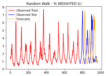
Figure 3. Percent of Weekly Patient Visits Exhibiting Influenza-Like Illness (ILI): Training (red), Testing (blue), RW (orange)

To help ensure a fair comparison, every new proposed model uses the codebase made public by the Informer model (Zhou et al., 2021) or one of the subsequent models based on it. This often involves using the same data-loading, transformation, and evaluation experimental setup. One, however, can observe some experimental or modeling differences, which can be summarized as follows:

• Look-back window: Early works on utilizing the Transformer model for forecasting used a relatively short look-back window, such as using a 96 look-back window to forecast 96, 192, 336, and 720 horizons for ETT datasets. The authors of (Zeng et al., 2023) explored increasing the look-back window for the Transformer-based models and found that the forecasting performance tends to degrade, falling short in utilizing the extended long temporal information. Alternatively, they showed that the PatchTST model benefits from the longer look-back window.

• Channel Mixing vs. Channel Independence: In channel mixing, the attention is applied to all the features projected into a shared embedding space. In channel-independence, the attention is applied separately to time points (or patches) in each channel, as in PatchTST, GPT4TS, and Time-LLM. One argument in favor of channel-independence is that each channel behaves differently, which can harm the overall performance when mixing all the channels. In addition, the authors of (Zhang and Yan, 2022) explored using two-stage attention: one for temporal attention and the other for cross-channel attention.

• Temporal Embeddings: For both cases (channel mixing and channel-independence), a modeling technique projects the features into an embedding space, and it can also use additional positional or temporal embeddings designed explicitly for each time frequency, such as weekly or hourly data. For instance, the Informer model utilizes three types of embeddings: feature, positional, and temporal embeddings. The PatchTST model uses two types: feature and positional. The GPT4TS model utilizes only one: the feature embeddings.

• Instance Normalization: Some modeling techniques also utilize the Reversible Instance Normalization (RevIN) (Kim et al., 2021), mitigating the distribution shift between the look-back window and the forecasting horizons. This technique simply normalizes the look-back window by subtracting the mean and dividing it by the standard deviation. Subsequently, a modeling technique is trained on those normalized look-back windows to generate the forecasting horizons. These forecasts then go through a denormalizing step to get the final forecasts for evaluation. This simpler technique has been proven effective and contributes to much of the gain of the PatchTST model and GPT4TS. For interested readers, please refer to Table 11 in the PatchTST paper for a detailed experiment on PatchTST with and without RevIN.

• Layer Normalization vs. Batch Normalization: Most Transformer-based modeling techniques, such as the Informer or Time-LLM models, use Layer Normalization for the attention heads. The PatchTST models, however, use batch normalization, which has been shown to improve the forecasting performance of the time series transformers (Zerveas et al., 2021).

• Residual Attention: In addition to the layer vs. batch normalization, the implementation of the attention block also varies across the Time Series Transformers. For example, the PatchTST model uses residual attention, which keeps attention scores and adds them to the attention scores in the next layer. The other models do not use any intermediate attention scores.

• Model Size: The modeling techniques under study vary substantially in the model size (model dimensions and layers) used for modeling. For example, the Informer uses two-layer attention blocks with the following parameters (d_model=512, n_heads=8, and d_ff=2048) for the ETTh1. PatchTST uses a three layers attention block with these parameters (d_model=16, n_heads=8, and d_ff=128). GPT4TS uses pre-trained GPT2 of the six layers with these parameters (d_model=768, n_heads=4, and d_ff=768) for the same dataset.

• On Baselines: To some extent, the modeling techniques are limited in their evaluation since they do not include simpler baselines that can sometimes be competitive, such as the Random Walk (RW), Mean Model (MM), or Simple Moving Average (SMA). These simple baselines serve as good starting points as they do not require any training, although SMA has a hyper-parameter (the window size or number of elements to average). For example, Figure 3 shows the Weighted (by age) Percentage of Patients with an ILI (for 966 time points) that has been divided into train (772) and test (194) sets. The forecasts (orange) are from the simple Random Walk (RW) baseline model and it tends to degrade with increasing forecasting horizons, unless it happened to match a cycle/period. In this case, the metrics for horizon = 24 weeks are [ N = 170, MSE = 10.046, MAE = 2.473, sMAPE = 89.490 ]. Note, these results are on the original scale as sMAPE values are distorted when data are standardized (or normalized). A note on reproducibility, since the baseline results are often collected in each new proposed model without actually rerunning the other models, it has been observed that some results are not reproducible by the research community in the GitHub repository of the models under study (although the results (e.g., MAE) tend to be close). In addition to the reproducibility, some researchers also observed a source of potential unfairness in the evaluations, as some test time steps are omitted during the data loading where some models use different batch sizes (e.g., skip the last incomplete batch). Although the effects are small, it would simply follow-on work if a standard could be followed. Furthermore, our testing has shown that small improvements in these models can be made by further tuning of the hyper-parameters (suggesting it might be useful to provide a standardized setting and improved setting).

Table 8 presents a comparative analysis of the modeling techniques under study on eight benchmark datasets. These models include LLM-based models (GPT4TS), Transformer-based models (PatchTST/42, FEDformer, Autoformer, Stationary, ETSformer, Informer, and Reformer), CNN-based model (TimesNet), and MLP-based models (NLinear, DLinear, and LightTS). The results are sourced from (Zeng et al., 2023; Zhou et al., 2023) and are generally consistent across different papers where each newly proposed model does not run the baselines but collects results from a previous paper. We included the models for which the code and hyper-parameters are made public, omitting PatchTST/64 for which the hyper-parameters for ILI are not available. The assessment employs MSE and MAE for the normalized observed and forecasted values, averaged over all features and forecasting horizons. The assessment shows that PatchTST consistently outperforms the other modeling techniques, such as GPT4TS which is based on a pre-trained LLM. PatchTST is also highly competitive with NLinear achieving comparable scores. Table 8 presents a rank of these models using the average MAE over all datasets and forecasting horizons.

One can observe that forecasting performance tends to be less variable on the Electricity and Traffic datasets for all the modeling techniques including the Informer and the Reformer models. However, the forecasting performance tends to be highly variable on the ETT and ILI datasets especially with Informer and Reformer being the least favorable models.

Table 8. Comparison of models using different look-back windows for forecasting {24, 36, 48, 60} horizons for ILI and {96, 192, 336, 720} for the other datasets. The evaluation metrics used are Mean Squared Error (MSE) and Mean Absolute Error (MAE) applied to the normalized observed and forecasted values. The lower the scores the better the forecast performance. The best scores are highlighted in bold.

Rank		3		2		5		1		4		8		9		6		7		10		11		12
Methods		GPT2(6)		NLinear		DLinear		PatchTST/42		TimesNet		FEDformer		Autoformer		Stationary		ETSformer		LightTS		Informer		Reformer
	Metrics	MSE	MAE	MSE	MAE	MSE	MAE	MSE	MAE	MSE	MAE	MSE	MAE	MSE	MAE	MSE	MAE	MSE	MAE	MSE	MAE	MSE	MAE	MSE	MAE
Weather	96	0.162	0.212	0.182	0.232	0.176	0.237	0.152	0.199	0.172	0.220	0.217	0.296	0.266	0.336	0.173	0.223	0.197	0.281	0.182	0.242	0.300	0.384	0.689	0.596
	192	0.204	0.248	0.225	0.269	0.220	0.282	0.197	0.243	0.219	0.261	0.276	0.336	0.307	0.367	0.245	0.285	0.237	0.312	0.227	0.287	0.598	0.544	0.752	0.638
	336	0.254	0.286	0.271	0.301	0.265	0.319	0.249	0.283	0.280	0.306	0.339	0.380	0.359	0.395	0.321	0.338	0.298	0.353	0.282	0.334	0.578	0.523	0.639	0.596
	720	0.326	0.337	0.338	0.348	0.333	0.362	0.320	0.335	0.365	0.359	0.403	0.428	0.419	0.428	0.414	0.410	0.352	0.288	0.352	0.386	1.059	0.741	1.130	0.792
	Avg	0.237	0.270	0.254	0.287	0.248	0.300	0.229	0.265	0.259	0.287	0.309	0.360	0.338	0.382	0.288	0.314	0.271	0.334	0.261	0.312	0.634	0.548	0.803	0.656
ETTh1	96	0.376	0.397	0.374	0.394	0.375	0.399	0.375	0.399	0.384	0.402	0.376	0.419	0.449	0.459	0.513	0.491	0.494	0.479	0.424	0.432	0.865	0.713	0.837	0.728
	192	0.416	0.418	0.408	0.415	0.405	0.416	0.414	0.421	0.436	0.429	0.420	0.448	0.500	0.482	0.534	0.504	0.538	0.504	0.475	0.462	1.008	0.792	0.923	0.766
	336	0.442	0.433	0.429	0.427	0.439	0.443	0.431	0.436	0.491	0.469	0.459	0.465	0.521	0.496	0.588	0.535	0.574	0.521	0.518	0.488	1.107	0.809	1.097	0.835
	720	0.477	0.456	0.440	0.453	0.472	0.490	0.449	0.466	0.521	0.500	0.506	0.507	0.514	0.512	0.643	0.616	0.562	0.535	0.547	0.533	1.181	0.865	1.257	0.889
	Avg	0.427	0.426	0.413	0.422	0.422	0.437	0.417	0.430	0.458	0.450	0.440	0.460	0.496	0.487	0.570	0.537	0.542	0.510	0.491	0.479	1.040	0.795	1.029	0.805
ETTh2	96	0.285	0.342	0.277	0.338	0.289	0.353	0.274	0.336	0.340	0.374	0.358	0.397	0.346	0.388	0.476	0.458	0.340	0.391	0.397	0.437	3.755	1.525	2.626	1.317
	192	0.354	0.389	0.344	0.381	0.383	0.418	0.339	0.379	0.402	0.414	0.429	0.439	0.456	0.452	0.512	0.493	0.430	0.439	0.520	0.504	5.602	1.931	11.12	2.979
	336	0.373	0.407	0.357	0.400	0.448	0.465	0.331	0.380	0.452	0.452	0.496	0.487	0.482	0.486	0.552	0.551	0.485	0.479	0.626	0.559	4.721	1.835	9.323	2.769
	720	0.406	0.441	0.394	0.436	0.605	0.551	0.379	0.422	0.462	0.468	0.463	0.474	0.515	0.511	0.562	0.560	0.500	0.497	0.863	0.672	3.647	1.625	3.874	1.697
	Avg	0.354	0.394	0.343	0.389	0.431	0.446	0.330	0.379	0.414	0.427	0.437	0.449	0.450	0.459	0.526	0.516	0.439	0.452	0.602	0.543	4.431	1.729	6.736	2.191
ETTm1	96	0.292	0.346	0.306	0.348	0.299	0.343	0.290	0.342	0.338	0.375	0.379	0.419	0.505	0.475	0.386	0.398	0.375	0.398	0.374	0.400	0.672	0.571	0.538	0.528
	192	0.332	0.372	0.349	0.375	0.335	0.365	0.332	0.369	0.374	0.387	0.426	0.441	0.553	0.496	0.459	0.444	0.408	0.410	0.400	0.407	0.795	0.669	0.658	0.592
	336	0.366	0.394	0.375	0.388	0.369	0.386	0.366	0.392	0.410	0.411	0.445	0.459	0.621	0.537	0.495	0.464	0.435	0.428	0.438	0.438	1.212	0.871	0.898	0.721
	720	0.417	0.421	0.433	0.422	0.425	0.421	0.420	0.424	0.478	0.450	0.543	0.490	0.671	0.561	0.585	0.516	0.499	0.462	0.527	0.502	1.166	0.823	1.102	0.841
	Avg	0.352	0.383	0.365	0.383	0.388	0.403	0.357	0.378	0.352	0.382	0.400	0.406	0.448	0.452	0.481	0.456	0.429	0.425	0.435	0.437	0.961	0.734	0.799	0.671
ETTm2	96	0.173	0.262	0.167	0.255	0.167	0.269	0.165	0.255	0.187	0.267	0.203	0.287	0.255	0.339	0.192	0.274	0.189	0.280	0.209	0.308	0.365	0.453	0.658	0.619
	192	0.229	0.301	0.221	0.293	0.224	0.303	0.220	0.292	0.249	0.309	0.269	0.328	0.281	0.340	0.280	0.339	0.253	0.319	0.311	0.382	0.533	0.563	1.078	0.827
	336	0.286	0.341	0.274	0.327	0.281	0.342	0.278	0.329	0.321	0.351	0.325	0.366	0.339	0.372	0.334	0.361	0.314	0.357	0.442	0.466	1.363	0.887	1.549	0.972
	720	0.378	0.401	0.368	0.384	0.397	0.421	0.367	0.385	0.408	0.403	0.421	0.415	0.433	0.432	0.417	0.413	0.414	0.413	0.675	0.587	3.379	1.338	2.631	1.242
	Avg	0.266	0.326	0.257	0.315	0.267	0.333	0.257	0.315	0.291	0.333	0.305	0.349	0.327	0.371	0.306	0.347	0.293	0.342	0.409	0.436	1.410	0.810	1.479	0.915
ILI	24	2.063	0.881	1.683	0.858	2.215	1.081	1.522	0.814	2.317	0.934	3.228	1.260	3.483	1.287	2.294	0.945	2.527	1.020	8.313	2.144	5.764	1.677	4.400	1.382
	36	1.868	0.892	1.703	0.859	1.963	0.963	1.430	0.834	1.972	0.920	2.679	1.080	3.103	1.148	1.825	0.848	2.615	1.007	6.631	1.902	4.755	1.467	4.783	1.448
	48	1.790	0.884	1.719	0.884	2.130	1.024	1.673	0.854	2.238	0.940	2.622	1.078	2.669	1.085	2.010	0.900	2.359	0.972	7.299	1.982	4.763	1.469	4.832	1.465
	60	1.979	0.957	1.819	0.917	2.368	1.096	1.529	0.862	2.027	0.928	2.857	1.157	2.770	1.125	2.178	0.963	2.487	1.016	7.283	1.985	5.264	1.564	4.882	1.483
	Avg	1.925	0.903	1.731	0.879	2.169	1.041	1.538	0.841	2.139	0.931	2.847	1.144	3.006	1.161	2.077	0.914	2.497	1.004	7.382	2.003	5.137	1.544	4.724	1.445
Electricity	96	0.139	0.238	0.141	0.237	0.140	0.237	0.130	0.222	0.168	0.272	0.193	0.308	0.201	0.317	0.169	0.273	0.187	0.304	0.207	0.307	0.274	0.368	0.312	0.402
	192	0.153	0.251	0.154	0.248	0.153	0.249	0.148	0.240	0.184	0.289	0.201	0.315	0.222	0.334	0.182	0.286	0.199	0.315	0.213	0.316	0.296	0.386	0.348	0.433
	336	0.169	0.266	0.171	0.265	0.169	0.267	0.167	0.261	0.198	0.300	0.214	0.329	0.231	0.338	0.200	0.304	0.212	0.329	0.230	0.333	0.300	0.394	0.350	0.433
	720	0.206	0.297	0.210	0.297	0.203	0.301	0.202	0.291	0.220	0.320	0.246	0.355	0.254	0.361	0.222	0.321	0.233	0.345	0.265	0.360	0.373	0.439	0.340	0.420
	Avg	0.167	0.263	0.169	0.268	0.166	0.263	0.162	0.253	0.192	0.295	0.214	0.327	0.227	0.338	0.193	0.296	0.208	0.323	0.229	0.329	0.311	0.397	0.338	0.422
Traffic	96	0.388	0.282	0.410	0.279	0.410	0.282	0.367	0.251	0.593	0.321	0.587	0.366	0.613	0.388	0.612	0.338	0.607	0.392	0.615	0.391	0.719	0.391	0.732	0.423
	192	0.407	0.290	0.423	0.284	0.423	0.287	0.385	0.259	0.617	0.336	0.604	0.373	0.616	0.382	0.613	0.340	0.621	0.399	0.601	0.382	0.696	0.379	0.733	0.420
	336	0.412	0.294	0.435	0.290	0.436	0.296	0.398	0.265	0.629	0.336	0.621	0.383	0.622	0.337	0.618	0.328	0.622	0.396	0.613	0.386	0.777	0.420	0.742	0.420
	720	0.450	0.312	0.464	0.307	0.466	0.315	0.434	0.287	0.640	0.350	0.626	0.382	0.660	0.408	0.653	0.355	0.632	0.396	0.658	0.407	0.864	0.472	0.755	0.423
	Avg	0.414	0.294	0.433	0.289	0.433	0.295	0.396	0.265	0.619	0.336	0.610	0.376	0.628	0.379	0.624	0.340	0.621	0.396	0.622	0.392	0.764	0.416	0.741	0.422
	Avg All	0.516	0.407	0.490	0.400	0.562	0.436	0.460	0.391	0.596	0.433	0.701	0.489	0.757	0.511	0.633	0.465	0.662	0.473	1.303	0.616	1.836	0.871	2.081	0.954

8. Summary

The second wave of progress on multivariate time series forecasting has been recent and appears to be heating up with the use of advanced deep learning architectures. Work has started to establish further improvements using Knowledge Graphs and Large Language Models. Efforts have started to train them with scientific literature, such as the CORD-19 dataset for COVID-19. A complete investigation of how this can help with time series forecasting or related problems of time series classification or anomaly detection will take some time. Analysis of the features/factors influencing the course/time evolution of a pandemic may be conducted with the help of LLMs. Findings from the analysis of a dataset (e.g., the effectiveness of mask policies) can be quickly checked against previous studies. New research can more quickly be suggested to fill gaps in existing knowledge. Established knowledge can be associated with knowledge graphs or temporal knowledge graphs. As discussed, there are multiple ways in which knowledge can be used to improve forecasting.

Foundation models are being created for several modalities of data and time series data are no exception. During the Fall of 2023, several foundation models for time series data were created and tested. They show promise for providing more accurate and robust forecasts as well as potential for greater explainability. As discussed, there are multiple options for backbone models as well as many choices for architectural elements. Although successful elements from LLMs are a good starting point, additional research is needed to optimize them for time series data.

Further potential is provided by multi-modal foundation models, where we emphasize the importance of modeling time series data with textual data. It is challenging to build time series foundation models that are comparable to existing large language models since: (1) unlike natural languages, existing time series data lacks the inherent semantic richness; (2) the semantics in time series data are often heavily domain-specific (e.g., the modeling of electrocardiogram signals would provide little help in predicting stock prices). There are several potential benefits of the multi-model modeling: (1) textual data can provide essential context that is not captured in the raw time series data; (2) textual semantics can provide domain-specific knowledge that enhances the model’s interpretability; (3) textual data can introduce additional features and dimensions of variability, which can help in training more robust and generalizable models. In this way, text-enhanced time series models can be more easily transferred across different tasks (e.g., classification, forecasting, anomaly detection) and domains. Recently, foundation models like Contrastive Language-Image Pre-Training (CLIP) (Radford et al., 2021) can effectively learn visual concepts from natural language supervision, which shows the success of data augmentation with textual semantics.

The scalation/data GitHub repository https://github.com/scalation/data contains links to datasets, knowledge graphs, models, code, and papers on time series forecasting. As the MSE and MAE values in this paper are based on normalized values and therefore hard to interpret (other than by looking at the relative scores), tables in scalation/data show MSE, MAE, and sMAPE quality metrics for the same forecasting models on the original scale. Results for COVID-19 pandemic prediction are also given in this repository.

References

- (1)
- Ainslie et al. (2023) Joshua Ainslie, James Lee-Thorp, Michiel de Jong, Yury Zemlyanskiy, Federico Lebrón, and Sumit Sanghai. 2023. GQA: Training Generalized Multi-Query Transformer Models from Multi-Head Checkpoints. arXiv preprint arXiv:2305.13245 (2023).
- Aldosari and Miller (2023) Mohammed Aldosari and John A Miller. 2023. On Transformer Autoregressive Decoding for Multivariate Time Series Forecasting. In European Symposium on Artificial Neural Networks, Computational Intelligence and Machine Learning (Bruges, Belgium).
- Athanasopoulos and Vahid (2008) George Athanasopoulos and Farshid Vahid. 2008. VARMA versus VAR for macroeconomic forecasting. Journal of Business & Economic Statistics 26, 2 (2008), 237–252.
- Bagnall et al. (2018) Anthony Bagnall, Hoang Anh Dau, Jason Lines, Michael Flynn, James Large, Aaron Bostrom, Paul Southam, and Eamonn Keogh. 2018. The UEA multivariate time series classification archive, 2018. arXiv preprint arXiv:1811.00075 (2018).
- Bai et al. (2022) Jiangang Bai, Yujing Wang, Hong Sun, Ruonan Wu, Tianmeng Yang, Pengfei Tang, Defu Cao, Mingliang Zhang, Yunhai Tong, Yaming Yang, et al. 2022. Enhancing self-attention with knowledge-assisted attention maps. In Proceedings of the 2022 Conference of the North American Chapter of the Association for Computational Linguistics: Human Language Technologies. 107–115.
- Bai et al. (2018) Shaojie Bai, J Zico Kolter, and Vladlen Koltun. 2018. An empirical evaluation of generic convolutional and recurrent networks for sequence modeling. arXiv preprint arXiv:1803.01271 (2018).
- Bengio et al. (2013) Yoshua Bengio, Aaron Courville, and Pascal Vincent. 2013. Representation learning: A review and new perspectives. IEEE transactions on pattern analysis and machine intelligence 35, 8 (2013), 1798–1828.
- Bommasani et al. (2021) Rishi Bommasani, Drew A Hudson, Ehsan Adeli, Russ Altman, Simran Arora, Sydney von Arx, Michael S Bernstein, Jeannette Bohg, Antoine Bosselut, Emma Brunskill, et al. 2021. On the opportunities and risks of foundation models. arXiv preprint arXiv:2108.07258 (2021).
- Box and Jenkins (1962) George EP Box and Gwilym M Jenkins. 1962. Some statistical aspects of adaptive optimization and control. Journal of the Royal Statistical Society: Series B (Methodological) 24, 2 (1962), 297–331.
- Box and Jenkins (1970) George EP Box and Gwilym M Jenkins. 1970. Time Series Analysis Forecasting and Control. Technical Report. DTIC Document.
- Box et al. (1967) George EP Box, Gwilym M Jenkins, and DW Bacon. 1967. Models for Forecasting Seasonal and Non-Seasonal Time Series. Technical Report. Wisconsin Univ Madison Dept of Statistics.
- Cao et al. (2023) Defu Cao, Furong Jia, Sercan O Arik, Tomas Pfister, Yixiang Zheng, Wen Ye, and Yan Liu. 2023. TEMPO: Prompt-based Generative Pre-trained Transformer for Time Series Forecasting. arXiv preprint arXiv:2310.04948 (2023).
- Cao et al. (2020) Defu Cao, Yujing Wang, Juanyong Duan, Ce Zhang, Xia Zhu, Congrui Huang, Yunhai Tong, Bixiong Xu, Jing Bai, Jie Tong, et al. 2020. Spectral temporal graph neural network for multivariate time-series forecasting. Advances in neural information processing systems 33 (2020), 17766–17778.
- Chang et al. (2023) Ching Chang, Wen-Chih Peng, and Tien-Fu Chen. 2023. Llm4ts: Two-stage fine-tuning for time-series forecasting with pre-trained llms. arXiv preprint arXiv:2308.08469 (2023).
- Chefer et al. (2021) Hila Chefer, Shir Gur, and Lior Wolf. 2021. Transformer interpretability beyond attention visualization. In Proceedings of the IEEE/CVF conference on computer vision and pattern recognition. 782–791.
- Cho et al. (2014) Kyunghyun Cho, Bart Van Merriënboer, Caglar Gulcehre, Dzmitry Bahdanau, Fethi Bougares, Holger Schwenk, and Yoshua Bengio. 2014. Learning phrase representations using RNN encoder-decoder for statistical machine translation. arXiv preprint arXiv:1406.1078 (2014).
- Chorowski et al. (2014) Jan Chorowski, Dzmitry Bahdanau, Kyunghyun Cho, and Yoshua Bengio. 2014. End-to-end continuous speech recognition using attention-based recurrent NN: First results. arXiv preprint arXiv:1412.1602 (2014).
- Cirstea et al. (2022) Razvan-Gabriel Cirstea, Chenjuan Guo, Bin Yang, Tung Kieu, Xuanyi Dong, and Shirui Pan. 2022. Triformer: Triangular, Variable-Specific Attentions for Long Sequence Multivariate Time Series Forecasting–Full Version. arXiv preprint arXiv:2204.13767 (2022).
- Cochrane and Orcutt (1949) Donald Cochrane and Guy H Orcutt. 1949. Application of least squares regression to relationships containing auto-correlated error terms. Journal of the American statistical association 44, 245 (1949), 32–61.
- Das et al. (2023) Abhimanyu Das, Weihao Kong, Rajat Sen, and Yichen Zhou. 2023. A decoder-only foundation model for time-series forecasting. arXiv preprint arXiv:2310.10688 (2023).
- Dau et al. (2019) Hoang Anh Dau, Anthony Bagnall, Kaveh Kamgar, Chin-Chia Michael Yeh, Yan Zhu, Shaghayegh Gharghabi, Chotirat Ann Ratanamahatana, and Eamonn Keogh. 2019. The UCR time series archive. IEEE/CAA Journal of Automatica Sinica 6, 6 (2019), 1293–1305.
- Ekambaram et al. (2023) Vijay Ekambaram, Arindam Jati, Nam Nguyen, Phanwadee Sinthong, and Jayant Kalagnanam. 2023. TSMixer: Lightweight MLP-Mixer Model for Multivariate Time Series Forecasting. arXiv preprint arXiv:2306.09364 (2023).
- Fritz et al. (2022) Cornelius Fritz, Emilio Dorigatti, and David Rügamer. 2022. Combining graph neural networks and spatio-temporal disease models to improve the prediction of weekly COVID-19 cases in Germany. Scientific Reports 12, 1 (2022), 3930.
- Fu et al. (2023) Zihao Fu, Wai Lam, Qian Yu, Anthony Man-Cho So, Shengding Hu, Zhiyuan Liu, and Nigel Collier. 2023. Decoder-Only or Encoder-Decoder? Interpreting Language Model as a Regularized Encoder-Decoder. arXiv preprint arXiv:2304.04052 (2023).
- Gao et al. (2023) Yunfan Gao, Yun Xiong, Xinyu Gao, Kangxiang Jia, Jinliu Pan, Yuxi Bi, Yi Dai, Jiawei Sun, and Haofen Wang. 2023. Retrieval-augmented generation for large language models: A survey. arXiv preprint arXiv:2312.10997 (2023).
- Garza and Mergenthaler-Canseco (2023) Azul Garza and Max Mergenthaler-Canseco. 2023. TimeGPT-1. arXiv preprint arXiv:2310.03589 (2023).
- Gilmer et al. (2017) Justin Gilmer, Samuel S Schoenholz, Patrick F Riley, Oriol Vinyals, and George E Dahl. 2017. Neural message passing for quantum chemistry. In International conference on machine learning. PMLR, 1263–1272.
- Godahewa et al. (2021) Rakshitha Godahewa, Christoph Bergmeir, Geoffrey I Webb, Rob J Hyndman, and Pablo Montero-Manso. 2021. Monash time series forecasting archive. arXiv preprint arXiv:2105.06643 (2021).
- Gordon et al. (2023) Emily M Gordon, Elizabeth A Barnes, James W Hurrell, Maria Rugenstein, Charles Anderson, et al. 2023. When is the Unpredictable (Slightly More) Predictable? An Assessment of Opportunities for Skillful Decadal Climate Prediction Using Explainable Neural Networks. (2023).
- Gu and Dao (2023) Albert Gu and Tri Dao. 2023. Mamba: Linear-time sequence modeling with selective state spaces. arXiv preprint arXiv:2312.00752 (2023).
- Gütebier et al. (2022) Lea Gütebier, Tim Bleimehl, Ron Henkel, Jamie Munro, Sebastian Müller, Axel Morgner, Jakob Laenge, Anke Pachauer, Alexander Erdl, Jens Weimar, et al. 2022. CovidGraph: a graph to fight COVID-19. Bioinformatics 38, 20 (2022), 4843–4845.
- Hamilton et al. (2017) Will Hamilton, Zhitao Ying, and Jure Leskovec. 2017. Inductive representation learning on large graphs. Advances in neural information processing systems 30 (2017).
- Han et al. (2023) Lu Han, Han-Jia Ye, and De-Chuan Zhan. 2023. The Capacity and Robustness Trade-off: Revisiting the Channel Independent Strategy for Multivariate Time Series Forecasting. arXiv preprint arXiv:2304.05206 (2023).
- He and Hofmann (2023) Bobby He and Thomas Hofmann. 2023. Simplifying Transformer Blocks. arXiv preprint arXiv:2311.01906 (2023).
- Hochreiter and Schmidhuber (1997) Sepp Hochreiter and Jürgen Schmidhuber. 1997. Long short-term memory. Neural computation 9, 8 (1997), 1735–1780.
- Holt Charles (1957) C Holt Charles. 1957. Forecasting trends and seasonal by exponentially weighted averages. International Journal of Forecasting 20, 1 (1957), 5–10.
- Houlsby et al. (2019) Neil Houlsby, Andrei Giurgiu, Stanislaw Jastrzebski, Bruna Morrone, Quentin De Laroussilhe, Andrea Gesmundo, Mona Attariyan, and Sylvain Gelly. 2019. Parameter-efficient transfer learning for NLP. In International Conference on Machine Learning. PMLR, 2790–2799.
- Hu et al. (2021) Edward J Hu, Yelong Shen, Phillip Wallis, Zeyuan Allen-Zhu, Yuanzhi Li, Shean Wang, Lu Wang, and Weizhu Chen. 2021. Lora: Low-rank adaptation of large language models. arXiv preprint arXiv:2106.09685 (2021).
- Hu et al. (2023) Linmei Hu, Zeyi Liu, Ziwang Zhao, Lei Hou, Liqiang Nie, and Juanzi Li. 2023. A Survey of Knowledge Enhanced Pre-Trained Language Models. IEEE Transactions on Knowledge and Data Engineering (2023).
- Hu et al. (2020) Ziniu Hu, Yuxiao Dong, Kuansan Wang, and Yizhou Sun. 2020. Heterogeneous graph transformer. In Proceedings of the web conference 2020. 2704–2710.
- Hyndman and Koehler (2006) Rob J Hyndman and Anne B Koehler. 2006. Another look at measures of forecast accuracy. International journal of forecasting 22, 4 (2006), 679–688.
- Javeri et al. (2021) Indrajeet Y Javeri, Mohammadhossein Toutiaee, Ismailcem B Arpinar, John A Miller, and Tom W Miller. 2021. Improving neural networks for time-series forecasting using data augmentation and AutoML. In 2021 IEEE Seventh International Conference on Big Data Computing Service and Applications (BigDataService). IEEE, 1–8.
- Jin et al. (2023a) Ming Jin, Huan Yee Koh, Qingsong Wen, Daniele Zambon, Cesare Alippi, Geoffrey I Webb, Irwin King, and Shirui Pan. 2023a. A survey on graph neural networks for time series: Forecasting, classification, imputation, and anomaly detection. arXiv preprint arXiv:2307.03759 (2023).
- Jin et al. (2023b) Ming Jin, Shiyu Wang, Lintao Ma, Zhixuan Chu, James Y Zhang, Xiaoming Shi, Pin-Yu Chen, Yuxuan Liang, Yuan-Fang Li, Shirui Pan, et al. 2023b. Time-llm: Time series forecasting by reprogramming large language models. arXiv preprint arXiv:2310.01728 (2023).
- Jin et al. (2022) Xiaoyong Jin, Youngsuk Park, Danielle Maddix, Hao Wang, and Yuyang Wang. 2022. Domain adaptation for time series forecasting via attention sharing. In International Conference on Machine Learning. PMLR, 10280–10297.
- Jones and Cox (1978) David Alan Jones and David Roxbee Cox. 1978. Nonlinear autoregressive processes. Proceedings of the Royal Society of London. A. Mathematical and Physical Sciences 360, 1700 (1978), 71–95.
- Jung et al. (2021) Jaehun Jung, Jinhong Jung, and U Kang. 2021. Learning to walk across time for interpretable temporal knowledge graph completion. In Proceedings of the 27th ACM SIGKDD Conference on Knowledge Discovery & Data Mining. 786–795.
- Kaplan et al. (2020) Jared Kaplan, Sam McCandlish, Tom Henighan, Tom B Brown, Benjamin Chess, Rewon Child, Scott Gray, Alec Radford, Jeffrey Wu, and Dario Amodei. 2020. Scaling laws for neural language models. arXiv preprint arXiv:2001.08361 (2020).
- Kapoor et al. (2020) Amol Kapoor, Xue Ben, Luyang Liu, Bryan Perozzi, Matt Barnes, Martin Blais, and Shawn O’Banion. 2020. Examining covid-19 forecasting using spatio-temporal graph neural networks. arXiv preprint arXiv:2007.03113 (2020).
- Karagiannakos (2021) Sergios Karagiannakos. 2021. Best Graph Neural Networks architectures: GCN, GAT, MPNN and more. https://theaisummer.com/gnn-architectures/. https://theaisummer.com/ (2021).
- Karniadakis et al. (2021) George Em Karniadakis, Ioannis G Kevrekidis, Lu Lu, Paris Perdikaris, Sifan Wang, and Liu Yang. 2021. Physics-informed machine learning. Nature Reviews Physics 3, 6 (2021), 422–440.
- Karpatne et al. (2017) Anuj Karpatne, Gowtham Atluri, James H Faghmous, Michael Steinbach, Arindam Banerjee, Auroop Ganguly, Shashi Shekhar, Nagiza Samatova, and Vipin Kumar. 2017. Theory-guided data science: A new paradigm for scientific discovery from data. IEEE Transactions on Knowledge and Data Engineering 29, 10 (2017), 2318–2331.
- Ke et al. (2017) Guolin Ke, Qi Meng, Thomas Finley, Taifeng Wang, Wei Chen, Weidong Ma, Qiwei Ye, and Tie-Yan Liu. 2017. Lightgbm: A highly efficient gradient boosting decision tree. Advances in neural information processing systems 30 (2017).
- Kim et al. (2023) Subin Kim, Euisuk Chung, and Pilsung Kang. 2023. FEAT: A general framework for feature-aware multivariate time-series representation learning. Knowledge-Based Systems 277 (2023), 110790.
- Kim et al. (2021) Taesung Kim, Jinhee Kim, Yunwon Tae, Cheonbok Park, Jang-Ho Choi, and Jaegul Choo. 2021. Reversible instance normalization for accurate time-series forecasting against distribution shift. In International Conference on Learning Representations.
- Kipf and Welling (2016) Thomas N Kipf and Max Welling. 2016. Semi-supervised classification with graph convolutional networks. arXiv preprint arXiv:1609.02907 (2016).
- Kitaev et al. (2020) Nikita Kitaev, Łukasz Kaiser, and Anselm Levskaya. 2020. Reformer: The efficient transformer. arXiv preprint arXiv:2001.04451 (2020).
- La Cava et al. (2018) William La Cava, Tilak Raj Singh, James Taggart, Srinivas Suri, and Jason H Moore. 2018. Learning concise representations for regression by evolving networks of trees. arXiv preprint arXiv:1807.00981 (2018).
- Lea et al. (2016) Colin Lea, Rene Vidal, Austin Reiter, and Gregory D Hager. 2016. Temporal convolutional networks: A unified approach to action segmentation. In European Conference on Computer Vision. Springer, 47–54.
- LeCun et al. (1995) Yann LeCun, Yoshua Bengio, et al. 1995. Convolutional networks for images, speech, and time series. The handbook of brain theory and neural networks 3361, 10 (1995), 1995.
- Li et al. (2019) Shiyang Li, Xiaoyong Jin, Yao Xuan, Xiyou Zhou, Wenhu Chen, Yu-Xiang Wang, and Xifeng Yan. 2019. Enhancing the locality and breaking the memory bottleneck of transformer on time series forecasting. Advances in neural information processing systems 32 (2019).
- Li et al. (2023b) Zhe Li, Zhongwen Rao, Lujia Pan, Pengyun Wang, and Zenglin Xu. 2023b. Ti-MAE: Self-Supervised Masked Time Series Autoencoders. arXiv preprint arXiv:2301.08871 (2023).
- Li et al. (2023a) Zhe Li, Zhongwen Rao, Lujia Pan, and Zenglin Xu. 2023a. Mts-mixers: Multivariate time series forecasting via factorized temporal and channel mixing. arXiv preprint arXiv:2302.04501 (2023).
- Liao et al. (2023) Baohao Liao, Yan Meng, and Christof Monz. 2023. Parameter-Efficient Fine-Tuning without Introducing New Latency. arXiv preprint arXiv:2305.16742 (2023).
- Lim and Zohren (2021) Bryan Lim and Stefan Zohren. 2021. Time-series forecasting with deep learning: a survey. Philosophical Transactions of the Royal Society A 379, 2194 (2021), 20200209.
- Lin et al. (2022) Tianyang Lin, Yuxin Wang, Xiangyang Liu, and Xipeng Qiu. 2022. A survey of transformers. AI Open (2022).
- Lin et al. (2020) Xuan Lin, Zhe Quan, Zhi-Jie Wang, Tengfei Ma, and Xiangxiang Zeng. 2020. KGNN: Knowledge Graph Neural Network for Drug-Drug Interaction Prediction.. In IJCAI, Vol. 380. 2739–2745.
- Liu and Nocedal (1989) Dong C Liu and Jorge Nocedal. 1989. On the limited memory BFGS method for large scale optimization. Mathematical programming 45, 1-3 (1989), 503–528.
- Liu et al. (2023b) Jiawei Liu, Cheng Yang, Zhiyuan Lu, Junze Chen, Yibo Li, Mengmei Zhang, Ting Bai, Yuan Fang, Lichao Sun, Philip S Yu, et al. 2023b. Towards graph foundation models: A survey and beyond. arXiv preprint arXiv:2310.11829 (2023).
- Liu et al. (2021) Shizhan Liu, Hang Yu, Cong Liao, Jianguo Li, Weiyao Lin, Alex X Liu, and Schahram Dustdar. 2021. Pyraformer: Low-complexity pyramidal attention for long-range time series modeling and forecasting. In International conference on learning representations.
- Liu et al. (2023a) Xu Liu, Junfeng Hu, Yuan Li, Shizhe Diao, Yuxuan Liang, Bryan Hooi, and Roger Zimmermann. 2023a. UniTime: A Language-Empowered Unified Model for Cross-Domain Time Series Forecasting. arXiv preprint arXiv:2310.09751 (2023).
- Liu et al. (2022) Yong Liu, Haixu Wu, Jianmin Wang, and Mingsheng Long. 2022. Non-stationary transformers: Exploring the stationarity in time series forecasting. Advances in Neural Information Processing Systems 35 (2022), 9881–9893.
- Ma et al. (2020) Yunshan Ma, Yujuan Ding, Xun Yang, Lizi Liao, Wai Keung Wong, and Tat-Seng Chua. 2020. Knowledge enhanced neural fashion trend forecasting. In Proceedings of the 2020 international conference on multimedia retrieval. 82–90.
- Makridakis et al. (2018) Spyros Makridakis, Evangelos Spiliotis, and Vassilios Assimakopoulos. 2018. The M4 Competition: Results, findings, conclusion and way forward. International Journal of Forecasting 34, 4 (2018), 802–808.
- Makridakis et al. (2022) Spyros Makridakis, Evangelos Spiliotis, and Vassilios Assimakopoulos. 2022. M5 accuracy competition: Results, findings, and conclusions. International Journal of Forecasting 38, 4 (2022), 1346–1364.
- Makridakis et al. (2023) Spyros Makridakis, Evangelos Spiliotis, Ross Hollyman, Fotios Petropoulos, Norman Swanson, and Anil Gaba. 2023. The M6 forecasting competition: Bridging the gap between forecasting and investment decisions. arXiv preprint arXiv:2310.13357 (2023).
- McIntosh et al. (2023) Timothy R McIntosh, Teo Susnjak, Tong Liu, Paul Watters, and Malka N Halgamuge. 2023. From Google Gemini to OpenAI Q*(Q-Star): A Survey of Reshaping the Generative Artificial Intelligence (AI) Research Landscape. arXiv preprint arXiv:2312.10868 (2023).
- Meng et al. (2023) Qianwen Meng, Hangwei Qian, Yong Liu, Yonghui Xu, Zhiqi Shen, and Lizhen Cui. 2023. Unsupervised Representation Learning for Time Series: A Review. arXiv preprint arXiv:2308.01578 (2023).
- Michel et al. (2020) Franck Michel, Fabien Gandon, Valentin Ah-Kane, Anna Bobasheva, Elena Cabrio, Olivier Corby, Raphaël Gazzotti, Alain Giboin, Santiago Marro, Tobias Mayer, et al. 2020. Covid-on-the-Web: Knowledge graph and services to advance COVID-19 research. In The Semantic Web–ISWC 2020: 19th International Semantic Web Conference, Athens, Greece, November 2–6, 2020, Proceedings, Part II 19. Springer, 294–310.
- Miller et al. (2023) John A. Miller, Nasid Habib Barna, Subas Rana, I. Budak Arpinar, and Ninghao Liu. 2023. Knowledge Enhanced Deep Learning: Application to Pandemic Prediction. In Proceedings of the 9th IEEE International Conference on Collaboration and Internet Computin. 1–10.
- Miller et al. (2010) John A Miller, Jun Han, and Maria Hybinette. 2010. Using domain specific language for modeling and simulation: Scalation as a case study. In The 2010 Winter Simulation Conference (WSC). ACM/IEEE, 741–752.
- Miller et al. (2017) John A Miller, Hao Peng, and Michael E Cotterell. 2017. Adding Support for Theory in Open Science Big Data. In the 6th IEEE International Congress on Big Data (BigData’17). IEEE, 251–255.
- Min et al. (2021) Bonan Min, Hayley Ross, Elior Sulem, Amir Pouran Ben Veyseh, Thien Huu Nguyen, Oscar Sainz, Eneko Agirre, Ilana Heintz, and Dan Roth. 2021. Recent advances in natural language processing via large pre-trained language models: A survey. Comput. Surveys (2021).
- Mrini et al. (2019) Khalil Mrini, Franck Dernoncourt, Quan Tran, Trung Bui, Walter Chang, and Ndapa Nakashole. 2019. Rethinking self-attention: Towards interpretability in neural parsing. arXiv preprint arXiv:1911.03875 (2019).
- Müller et al. (1997) K-R Müller, Alexander J Smola, Gunnar Rätsch, Bernhard Schölkopf, Jens Kohlmorgen, and Vladimir Vapnik. 1997. Predicting time series with support vector machines. In International Conference on Artificial Neural Networks. Springer, 999–1004.
- Müller (2007) Meinard Müller. 2007. Dynamic time warping. Information retrieval for music and motion (2007), 69–84.
- Nie et al. (2022) Yuqi Nie, Nam H Nguyen, Phanwadee Sinthong, and Jayant Kalagnanam. 2022. A time series is worth 64 words: Long-term forecasting with transformers. arXiv preprint arXiv:2211.14730 (2022).
- Oreshkin et al. (2019) Boris N Oreshkin, Dmitri Carpov, Nicolas Chapados, and Yoshua Bengio. 2019. N-BEATS: Neural basis expansion analysis for interpretable time series forecasting. arXiv preprint arXiv:1905.10437 (2019).
- Pai and Liu (2018) Ping-Feng Pai and Chia-Hsin Liu. 2018. Predicting vehicle sales by sentiment analysis of twitter data and stock market values. IEEE Access 6 (2018), 57655–57662.
- Palaskar et al. (2023) Santosh Palaskar, Vijay Ekambaram, Arindam Jati, Neelamadhav Gantayat, Avirup Saha, Seema Nagar, Nam H Nguyen, Pankaj Dayama, Renuka Sindhgatta, Prateeti Mohapatra, et al. 2023. AutoMixer for Improved Multivariate Time-Series Forecasting on BizITOps Data. arXiv preprint arXiv:2310.20280 (2023).
- Panagopoulos et al. (2021) George Panagopoulos, Giannis Nikolentzos, and Michalis Vazirgiannis. 2021. Transfer graph neural networks for pandemic forecasting. In Proceedings of the AAAI Conference on Artificial Intelligence, Vol. 35. 4838–4845.
- Pearl (2011) Judea Pearl. 2011. Exogeneity and superexogeneity: a no-tear perspective. (2011).
- Peng et al. (2019) Hao Peng, Nicholas Klepp, Mohammadhossein Toutiaee, I Budak Arpinar, and John A Miller. 2019. Knowledge and Situation-Aware Vehicle Traffic Forecasting. In 2019 IEEE International Conference on Big Data (Big Data). IEEE, 3803–3812.
- Pestryakova et al. (2022) Svetlana Pestryakova, Daniel Vollmers, Mohamed Ahmed Sherif, Stefan Heindorf, Muhammad Saleem, Diego Moussallem, and Axel-Cyrille Ngonga Ngomo. 2022. Covidpubgraph: A fair knowledge graph of covid-19 publications. Scientific Data 9, 1 (2022), 389.
- Qi et al. (2021) Xinyuan Qi, Kai Hou, Tong Liu, Zhongzhong Yu, Sihao Hu, and Wenwu Ou. 2021. From known to unknown: Knowledge-guided transformer for time-series sales forecasting in Alibaba. arXiv preprint arXiv:2109.08381 (2021).
- Quenouille and Quenouille (1957) Maurice Henry Quenouille and MH Quenouille. 1957. The analysis of multiple time-series. Technical Report. Griffin London.
- Radford et al. (2021) Alec Radford, Jong Wook Kim, Chris Hallacy, Aditya Ramesh, Gabriel Goh, Sandhini Agarwal, Girish Sastry, Amanda Askell, Pamela Mishkin, Jack Clark, et al. 2021. Learning transferable visual models from natural language supervision. In International conference on machine learning. PMLR, 8748–8763.
- Ramsay and Dalzell (1991) James O Ramsay and CJ Dalzell. 1991. Some tools for functional data analysis. Journal of the Royal Statistical Society: Series B (Methodological) 53, 3 (1991), 539–561.
- Rana et al. (2023) Subas Rana, Nasid Habib Barna, and John A Miller. 2023. Exploring the Predictive Power of Correlation and Mutual Information in Attention Temporal Graph Convolutional Network for COVID-19 Forecasting. In International Conference on Big Data. Springer, 18–33.
- Rasul et al. (2023) Kashif Rasul, Arjun Ashok, Andrew Robert Williams, Arian Khorasani, George Adamopoulos, Rishika Bhagwatkar, Marin Biloš, Hena Ghonia, Nadhir Vincent Hassen, Anderson Schneider, et al. 2023. Lag-llama: Towards foundation models for time series forecasting. arXiv preprint arXiv:2310.08278 (2023).
- Rong et al. (2020) Yu Rong, Yatao Bian, Tingyang Xu, Weiyang Xie, Ying Wei, Wenbing Huang, and Junzhou Huang. 2020. Self-supervised graph transformer on large-scale molecular data. Advances in Neural Information Processing Systems 33 (2020), 12559–12571.
- Rose (2020) Peter Rose. 2020. Peter Rose: COVID-19-Net: Integrating Health, Pathogen and Environmental Data into a Knowledge Graph for Case Tracking, Analysis, and Forecasting. (2020).
- Rossi et al. (2020) Emanuele Rossi, Ben Chamberlain, Fabrizio Frasca, Davide Eynard, Federico Monti, and Michael Bronstein. 2020. Temporal graph networks for deep learning on dynamic graphs. arXiv preprint arXiv:2006.10637 (2020).
- Salinas et al. (2020) David Salinas, Valentin Flunkert, Jan Gasthaus, and Tim Januschowski. 2020. DeepAR: Probabilistic forecasting with autoregressive recurrent networks. International Journal of Forecasting 36, 3 (2020), 1181–1191.
- Scott Armstrong and Collopy (1993) J Scott Armstrong and Fred Collopy. 1993. Causal forces: Structuring knowledge for time-series extrapolation. Journal of Forecasting 12, 2 (1993), 103–115.
- Shazeer (2020) Noam Shazeer. 2020. Glu variants improve transformer. arXiv preprint arXiv:2002.05202 (2020).
- Singh and Balasundaram (2007) Rampal Singh and S Balasundaram. 2007. Application of extreme learning machine method for time series analysis. International Journal of Intelligent Technology 2, 4 (2007), 256–262.
- Smith et al. (1988) Jack W Smith, James E Everhart, WC Dickson, William C Knowler, and Robert Scott Johannes. 1988. Using the ADAP learning algorithm to forecast the onset of diabetes mellitus. In Proceedings of the annual symposium on computer application in medical care. American Medical Informatics Association, 261.
- Smyl (2020) Slawek Smyl. 2020. A hybrid method of exponential smoothing and recurrent neural networks for time series forecasting. International Journal of Forecasting 36, 1 (2020), 75–85.
- Sorscher et al. (2022) Ben Sorscher, Robert Geirhos, Shashank Shekhar, Surya Ganguli, and Ari Morcos. 2022. Beyond neural scaling laws: beating power law scaling via data pruning. Advances in Neural Information Processing Systems 35 (2022), 19523–19536.
- Steenwinckel et al. (2020) Bram Steenwinckel, Gilles Vandewiele, Ilja Rausch, Pieter Heyvaert, Ruben Taelman, Pieter Colpaert, Pieter Simoens, Anastasia Dimou, Filip De Turck, and Femke Ongenae. 2020. Facilitating the analysis of COVID-19 literature through a knowledge graph. In International Semantic Web Conference. Springer, 344–357.
- Su et al. (2024) Jianlin Su, Murtadha Ahmed, Yu Lu, Shengfeng Pan, Wen Bo, and Yunfeng Liu. 2024. Roformer: Enhanced transformer with rotary position embedding. Neurocomputing 568 (2024), 127063.
- Tang and Zhang (2022) Peiwang Tang and Xianchao Zhang. 2022. MTSMAE: Masked Autoencoders for Multivariate Time-Series Forecasting. In 2022 IEEE 34th International Conference on Tools with Artificial Intelligence (ICTAI). IEEE, 982–989.
- Thapak and Hore (2020) Prakhar Thapak and Prodip Hore. 2020. Transformer++. arXiv preprint arXiv:2003.04974 (2020).
- Tolstikhin et al. (2021) Ilya O Tolstikhin, Neil Houlsby, Alexander Kolesnikov, Lucas Beyer, Xiaohua Zhai, Thomas Unterthiner, Jessica Yung, Andreas Steiner, Daniel Keysers, Jakob Uszkoreit, et al. 2021. Mlp-mixer: An all-mlp architecture for vision. Advances in neural information processing systems 34 (2021), 24261–24272.
- Touvron et al. (2023a) Hugo Touvron, Thibaut Lavril, Gautier Izacard, Xavier Martinet, Marie-Anne Lachaux, Timothée Lacroix, Baptiste Rozière, Naman Goyal, Eric Hambro, Faisal Azhar, et al. 2023a. Llama: Open and efficient foundation language models. arXiv preprint arXiv:2302.13971 (2023).
- Touvron et al. (2023b) Hugo Touvron, Louis Martin, Kevin Stone, Peter Albert, Amjad Almahairi, Yasmine Babaei, Nikolay Bashlykov, Soumya Batra, Prajjwal Bhargava, Shruti Bhosale, et al. 2023b. Llama 2: Open foundation and fine-tuned chat models. arXiv preprint arXiv:2307.09288 (2023).
- Vaswani et al. (2017) Ashish Vaswani, Noam Shazeer, Niki Parmar, Jakob Uszkoreit, Llion Jones, Aidan N Gomez, Łukasz Kaiser, and Illia Polosukhin. 2017. Attention is all you need. Advances in neural information processing systems 30 (2017).
- Velickovic et al. (2017) Petar Velickovic, Guillem Cucurull, Arantxa Casanova, Adriana Romero, Pietro Lio, Yoshua Bengio, et al. 2017. Graph attention networks. stat 1050, 20 (2017), 10–48550.
- Wan et al. (2023) Zhongwei Wan, Xin Wang, Che Liu, Samiul Alam, Yu Zheng, Zhongnan Qu, Shen Yan, Yi Zhu, Quanlu Zhang, Mosharaf Chowdhury, et al. 2023. Efficient Large Language Models: A Survey. arXiv preprint arXiv:2312.03863 (2023).
- Wang et al. (2020a) Lijing Wang, Xue Ben, Aniruddha Adiga, Adam Sadilek, Ashish Tendulkar, Srinivasan Venkatramanan, Anil Vullikanti, Gaurav Aggarwal, Alok Talekar, Jiangzhuo Chen, et al. 2020a. Using mobility data to understand and forecast covid19 dynamics. MedRxiv (2020).
- Wang et al. (2020b) Shuo Wang, Yanran Li, Jiang Zhang, Qingye Meng, Lingwei Meng, and Fei Gao. 2020b. PM2. 5-GNN: A domain knowledge enhanced graph neural network for PM2. 5 forecasting. In Proceedings of the 28th international conference on advances in geographic information systems. 163–166.
- Wen et al. (2022) Qingsong Wen, Tian Zhou, Chaoli Zhang, Weiqi Chen, Ziqing Ma, Junchi Yan, and Liang Sun. 2022. Transformers in time series: A survey. arXiv preprint arXiv:2202.07125 (2022).
- Werner et al. (2023) Luisa Werner, Nabil Layaïda, Pierre Genevès, and Sarah Chlyah. 2023. Knowledge Enhanced Graph Neural Networks. arXiv preprint arXiv:2303.15487 (2023).
- Whittle (1951) Peter Whittle. 1951. Hypothesis testing in time series analysis. Vol. 4. Almqvist & Wiksells boktr.
- Williams and Zipser (1989) Ronald J Williams and David Zipser. 1989. A learning algorithm for continually running fully recurrent neural networks. Neural computation 1, 2 (1989), 270–280.
- Winters (1960) Peter R Winters. 1960. Forecasting Sales by Exponentially Weighted Moving Averages. Management science 6, 3 (1960), 324–342.
- Woo et al. (2022) Gerald Woo, Chenghao Liu, Doyen Sahoo, Akshat Kumar, and Steven Hoi. 2022. CoST: Contrastive learning of disentangled seasonal-trend representations for time series forecasting. arXiv preprint arXiv:2202.01575 (2022).
- Wu et al. (2022) Haixu Wu, Tengge Hu, Yong Liu, Hang Zhou, Jianmin Wang, and Mingsheng Long. 2022. Timesnet: Temporal 2d-variation modeling for general time series analysis. arXiv preprint arXiv:2210.02186 (2022).
- Wu et al. (2021) Haixu Wu, Jiehui Xu, Jianmin Wang, and Mingsheng Long. 2021. Autoformer: Decomposition transformers with auto-correlation for long-term series forecasting. Advances in Neural Information Processing Systems 34 (2021), 22419–22430.
- Xie et al. (2020) Jianwen Xie, Ruiqi Gao, Erik Nijkamp, Song-Chun Zhu, and Ying Nian Wu. 2020. Representation learning: A statistical perspective. Annual Review of Statistics and Its Application 7 (2020), 303–335.
- Xu et al. (2019) Chengjin Xu, Mojtaba Nayyeri, Fouad Alkhoury, Hamed Shariat Yazdi, and Jens Lehmann. 2019. Temporal knowledge graph embedding model based on additive time series decomposition. arXiv preprint arXiv:1911.07893 (2019).
- Xu et al. (2018) Keyulu Xu, Weihua Hu, Jure Leskovec, and Stefanie Jegelka. 2018. How powerful are graph neural networks? arXiv preprint arXiv:1810.00826 (2018).
- Xue and Salim (2023) Hao Xue and Flora D Salim. 2023. Promptcast: A new prompt-based learning paradigm for time series forecasting. IEEE Transactions on Knowledge and Data Engineering (2023).
- Yang et al. (2021) Jian Yang, Gang Xiao, Yulong Shen, Wei Jiang, Xinyu Hu, Ying Zhang, and Jinghui Peng. 2021. A survey of knowledge enhanced pre-trained models. arXiv preprint arXiv:2110.00269 (2021).
- Yang et al. (2022) Xinyu Yang, Zhenguo Zhang, and Rongyi Cui. 2022. Timeclr: A self-supervised contrastive learning framework for univariate time series representation. Knowledge-Based Systems 245 (2022), 108606.
- Yeh et al. (2023) Chin-Chia Michael Yeh, Xin Dai, Huiyuan Chen, Yan Zheng, Yujie Fan, Audrey Der, Vivian Lai, Zhongfang Zhuang, Junpeng Wang, Liang Wang, et al. 2023. Toward a foundation model for time series data. In Proceedings of the 32nd ACM International Conference on Information and Knowledge Management. 4400–4404.
- Ying et al. (2021) Chengxuan Ying, Tianle Cai, Shengjie Luo, Shuxin Zheng, Guolin Ke, Di He, Yanming Shen, and Tie-Yan Liu. 2021. Do transformers really perform badly for graph representation? Advances in Neural Information Processing Systems 34 (2021), 28877–28888.
- Yue et al. (2022) Zhihan Yue, Yujing Wang, Juanyong Duan, Tianmeng Yang, Congrui Huang, Yunhai Tong, and Bixiong Xu. 2022. TS2Vec: Towards universal representation of time series. In Proceedings of the AAAI Conference on Artificial Intelligence, Vol. 36. 8980–8987.
- Zeng et al. (2023) Ailing Zeng, Muxi Chen, Lei Zhang, and Qiang Xu. 2023. Are transformers effective for time series forecasting?. In Proceedings of the AAAI conference on artificial intelligence, Vol. 37. 11121–11128.
- Zerveas et al. (2021) George Zerveas, Srideepika Jayaraman, Dhaval Patel, Anuradha Bhamidipaty, and Carsten Eickhoff. 2021. A transformer-based framework for multivariate time series representation learning. In Proceedings of the 27th ACM SIGKDD conference on knowledge discovery & data mining. 2114–2124.
- Zha et al. (2022) Mengyue Zha, SiuTim Wong, Mengqi Liu, Tong Zhang, and Kani Chen. 2022. Time series generation with masked autoencoder. arXiv preprint arXiv:2201.07006 (2022).
- Zhang and Sennrich (2019) Biao Zhang and Rico Sennrich. 2019. Root mean square layer normalization. Advances in Neural Information Processing Systems 32 (2019).
- Zhang et al. (2023b) Kexin Zhang, Qingsong Wen, Chaoli Zhang, Rongyao Cai, Ming Jin, Yong Liu, James Zhang, Yuxuan Liang, Guansong Pang, Dongjin Song, et al. 2023b. Self-Supervised Learning for Time Series Analysis: Taxonomy, Progress, and Prospects. arXiv preprint arXiv:2306.10125 (2023).
- Zhang and Yan (2022) Yunhao Zhang and Junchi Yan. 2022. Crossformer: Transformer utilizing cross-dimension dependency for multivariate time series forecasting. In The Eleventh International Conference on Learning Representations.
- Zhang et al. (2023a) Zhenwei Zhang, Xin Wang, and Yuantao Gu. 2023a. Sageformer: Series-aware graph-enhanced transformers for multivariate time series forecasting. arXiv preprint arXiv:2307.01616 (2023).
- Zhao et al. (2023) Ziqi Zhao, Yucheng Shi, Shushan Wu, Fan Yang, Wenzhan Song, and Ninghao Liu. 2023. Interpretation of Time-Series Deep Models: A Survey. arXiv preprint arXiv:2305.14582 (2023).
- Zheng et al. (2023) Xiaochen Zheng, Xingyu Chen, Manuel Schürch, Amina Mollaysa, Ahmed Allam, and Michael Krauthammer. 2023. SimTS: Rethinking Contrastive Representation Learning for Time Series Forecasting. arXiv preprint arXiv:2303.18205 (2023).
- Zhou et al. (2016) Guo-Bing Zhou, Jianxin Wu, Chen-Lin Zhang, and Zhi-Hua Zhou. 2016. Minimal gated unit for recurrent neural networks. International Journal of Automation and Computing 13, 3 (2016), 226–234.
- Zhou et al. (2021) Haoyi Zhou, Shanghang Zhang, Jieqi Peng, Shuai Zhang, Jianxin Li, Hui Xiong, and Wancai Zhang. 2021. Informer: Beyond efficient transformer for long sequence time-series forecasting. In Proceedings of the AAAI conference on artificial intelligence, Vol. 35. 11106–11115.
- Zhou et al. (2022a) Tian Zhou, Ziqing Ma, Qingsong Wen, Liang Sun, Tao Yao, Wotao Yin, Rong Jin, et al. 2022a. FiLM: Frequency improved legendre memory model for long-term time series forecasting. Advances in Neural Information Processing Systems 35 (2022), 12677–12690.
- Zhou et al. (2022b) Tian Zhou, Ziqing Ma, Qingsong Wen, Xue Wang, Liang Sun, and Rong Jin. 2022b. FEDformer: Frequency enhanced decomposed transformer for long-term series forecasting. In International Conference on Machine Learning. PMLR, 27268–27286.
- Zhou et al. (2023) Tian Zhou, Peisong Niu, Xue Wang, Liang Sun, and Rong Jin. 2023. One Fits All: Power General Time Series Analysis by Pretrained LM. arXiv preprint arXiv:2302.11939 (2023).
- Zhu et al. (2023) Qingbo Zhu, Jialin Han, Kai Chai, and Cunsheng Zhao. 2023. Time Series Analysis Based on Informer Algorithms: A Survey. Symmetry 15, 4 (2023), 951.
- Zhu et al. (2022) Rui Zhu, Krzysztof Janowicz, Gengchen Mai, Ling Cai, and Meilin Shi. 2022. COVID-Forecast-Graph: An open knowledge graph for consolidating COVID-19 forecasts and economic indicators via place and time. AGILE: GIScience Series 3 (2022), 21.