Dynamical Generation of the Baryon Asymmetry from a Scale Hierarchy

Abstract

We propose a novel baryogenesis scenario where the baryon asymmetry originates directly from a hierarchy between two fundamental mass scales: the electroweak scale and the Planck scale. Our model is based on the neutrino-portal Affleck-Dine (AD) mechanism, which generates the asymmetry of the AD sector during the radiation-dominated era and subsequently transfers it to the baryon number before the electroweak phase transition. The observed baryon asymmetry is then a natural outcome of this scenario. The model is testable as it predicts the existence of a Majoron with a keV mass and an electroweak scale decay constant. The impact of the relic Majoron on $\Delta N_{\rm eff}$ can be measured through near-future CMB observations.

Introduction.—

The observed baryon asymmetry Aghanim et al. (2020) is often parameterized with

$$Y_{B}\equiv\frac{\bar{n}_{B}}{s}=(0.82-0.92)\times 10^{-10}\,,$$ (1)

where $\bar{n}_{B}$ is the net baryon number density and $s$ is the entropy density. This value is significantly larger than the baryon asymmetry naturally anticipated in the Standard Model (SM), requiring new physics beyond the SM. However, if the baryon asymmetry arises from new physics, it is essential to realize the observed baryon asymmetry with the model parameters of the new physics. Previous works have typically relied on small couplings or large wash-out effects to yield the observed baryon asymmetry Bodeker and Buchmuller (2021); Elor et al. (2022); Barrow et al. (2022).

In this Letter, we propose a scenario of baryogenesis where the baryon asymmetry results directly from a scale hierarchy between the two important mass scales in phenomenology: the electroweak scale $v=246$ GeV and the reduced Planck mass $M_{P}=2.4\times 10^{18}\mathrm{\;GeV}$, in the form of

$$Y_{B}={\cal O}(0.01)\sqrt{\frac{v}{M_{P}}}\sim 10^{-10}\,.$$ (2)

We utilize the Affleck-Dine (AD) mechanism Affleck and Dine (1985); Dine et al. (1996), where the asymmetry is generated from the dynamics of a $B-L$ charged complex scalar field $\phi$. $\phi$ naturally has an electroweak scale mass, $m_{\phi}={\cal O}(100\mathrm{\;GeV})$, if the scalar potential of $\phi$ is governed by the same mechanism that ensures the stability of the Higgs boson mass against quantum corrections. In contrast to previous works on AD baryogenesis Allahverdi and Mazumdar (2012), we explore the generation of $B-L$ asymmetry during the radiation-dominated era and its subsequent transfer to the SM sector through neutrino-portal interactions. Therefore in our scenario, there is no dependence on the reheating temperature.

A simple model realizing our scenario is constructed by employing supersymmetry (SUSY) sus (2000); Ellis et al. (1984); Nilles et al. (1983). The relevant interactions of the model in terms of superpotential are given by

$$W=y_{\nu}\ell hN+\frac{1}{2}\lambda_{N}\phi N^{2}+\frac{\kappa}{4M_{P}}\phi^{4}+\cdots\,,$$ (3)

where $\ell$ is the SM lepton doublet, $h$ is the Higgs field, $N$ is a right-handed (RH) neutrino with $B-L=1$, and $\phi$ is a SM singlet scalar field with $B-L=-2$. $y_{\nu}$ is the neutrino Yukawa coupling that gives neutrino masses $m_{\nu}$ through the seesaw mechanism Minkowski (1977); Ramond (1979); Gell-Mann et al. (1979); Yanagida (1979); Mohapatra and Senjanovic (1981), while $\lambda_{N}$ and $\kappa$ are $\mathcal{O}(1)$ coefficients. A global $U(1)_{B-L}$ symmetry is preserved at the renormalizable level, allowing only the seesaw operators, but is explicitly broken by Planck-scale suppressed operators as generally expected due to quantum gravity effects Holman et al. (1992); Kamionkowski and March-Russell (1992); Barr and Seckel (1992). We highlight how supersymmetry breaking can provide a well-organized scalar potential in the presence of explicit $U(1)_{B-L}$ breaking terms and show how the two fundamental mass scales are combined to determine the baryon asymmetry. Moreover, we establish an interesting connection between the observable dark radiation and the baryon asymmetry with certain implications of the electroweak scale, emerging as a generic prediction.

Summary of cosmological history.—

Initially, the SM plasma dominates the energy density of the Universe, while the abundances of the novel particles $\phi$ and $N$ are negligible. When the temperature drops to $T_{\rm AD}\sim\sqrt{m_{\phi}M_{P}}$, the AD mechanism becomes active, generating the asymmetry of $\phi$. The temperature continues to decrease, leading to the thermalization of the AD sector ($\phi$ and $N$) with the SM plasma at the temperature $T_{N}$ via the neutrino Yukawa interactions. Once thermalized, the asymmetry is transmitted to the lepton sector through the neutrino portal, and the baryon asymmetry is induced via the weak sphaleron process and frozen after the electroweak phase transition. After the $B-L$ phase transition happens, all novel particles decay to the Majoron $J$, the pseudo-Nambu-Goldstone boson associated with the spontaneous $U(1)_{B-L}$ breaking. The Majoron, along with its decay products, contributes to $\Delta N_{\textrm{eff}}$, providing a phenomenological signal for the model.

Asymmetry generation.—

With the field decomposition of $\phi=\frac{1}{\sqrt{2}}r_{\phi}e^{i\theta_{\phi}}$, the net charge density of the scalar field $\phi$ becomes

$$\bar{n}_{\phi}=i(\dot{\phi}^{*}\phi-\phi^{*}\dot{\phi})=r^{2}_{\phi}\dot{\theta}_{\phi}\,,$$ (4)

which can be interpreted as a rotating scalar field carrying angular momentum in the field space. In the early Universe, a nonzero charge density can arise from the “kick” along the $\theta_{\phi}$ direction induced by the $B-L$ breaking potential term for a large value of $r_{\phi}$. In addition to the supersymmetric contribution given by $|\partial W/\partial\phi|^{2}$, the scalar potential incorporates soft supersymmetry breaking terms Witten (1981); Dimopoulos and Georgi (1981); Susskind (1984); Girardello and Grisaru (1982); Hall and Randall (1990),

$$\Delta V_{\rm soft}=m_{\phi}^{2}|\phi|^{2}-\left(\alpha m_{\phi}W(\phi)+h.c.\right),$$ (5)

where the model-dependent constant $\alpha$ naturally assumes a value of ${\cal O}(0.1-1)$. Coupled to the SM fermions $\psi_{a}$ through the higher dimensional operator arising from the Kähler potential,

$$\Delta{\cal L}=\kappa_{a}\frac{|\phi|^{2}}{M_{P}^{2}}\bar{\psi}_{a}i\gamma^{\mu}D_{\mu}\psi_{a},$$ (6)

the field $\phi$ acquires an additional mass. During the radiation-dominated era, the above interaction generates an effective mass squared of $\phi$ proportional to $H^{2}=\rho_{\rm tot}/(3M_{P}^{2})=\pi^{2}g_{*}T^{4}/(90M_{P}^{2})$. Here $H$ is the Hubble expansion rate, and $g_{*}={\cal O}(100)$ is relativistic degrees of freedom. The overall coefficient of this Hubble term $\kappa_{H}$ is typically the order of unity Kawasaki and Takesako (2012). Including all these contributions, the relevant potential of $\phi$ is given by

$$\hskip-14.22636ptV=(m_{\phi}^{2}-\hskip-1.42271pt\kappa_{H}\hskip-1.42271ptH^{2})|\phi|^{2}-\frac{\kappa\alpha m_{\phi}}{4M_{P}}\left(\phi^{4}+\phi^{*4}\right)+\frac{\kappa^{2}}{M_{P}^{2}}|\phi|^{6}$$

$$\hskip-3.41418pt=\frac{1}{2}(m_{\phi}^{2}-\hskip-1.42271pt\kappa_{H}\hskip-1.42271ptH^{2})r^{2}_{\phi}-\frac{\kappa\alpha m_{\phi}}{8M_{P}}r^{4}_{\phi}\cos 4\theta_{\phi}+\frac{\kappa^{2}}{8M_{P}^{2}}r^{6}_{\phi}\,,$$

in the field basis where $\alpha$ is real. Here we take $m_{\phi}^{2}>0$ and $\kappa_{H}>0$. It is worth noting that, owing to supersymmetry, the quadratic term remains shielded from large quantum corrections while the $B-L$ breaking quartic term is highly suppressed by a factor of $m_{\phi}/M_{P}$, which are critical aspects in our scenario.

At high temperatures where $H\gg m_{\phi}$, the minimum of the potential is predominantly determined by the Hubble-induced mass term. Having a mass similar to $H$, the radial field $r_{\phi}(x)$ resides at

$$\langle r_{\phi}\rangle=\left(\frac{4\kappa_{H}}{3\kappa^{2}}\right)^{\frac{1}{4}}\sqrt{HM_{P}}\,.$$ (8)

On the other hand, the angular field $a(x)=\langle r_{\phi}\rangle\theta_{\phi}(x)$ has an effective mass smaller than $H$, resulting in its position in the field space being nearly frozen at an arbitrary value. As the Universe expands and $H$ decreases, the sign of the quadratic term inverts, and the scalar potential is lifted subsequently. Due to the rapid lifting compared to the Hubble time, there is an increase solely in the potential energy, with a negligible change in the radial field value. As the quadratic term approaches zero, the quartic potential term imparts a mass of $\mathcal{O}(H)$ to the angular field. Then, for a typical value of $\theta_{\textrm{in}}$, an initial misalignment angle of $\theta_{\phi}$, the angular field starts to roll toward the minimum. However, with the diminishing radial field value due to rolling, the potential barrier height along the radial direction also decreases, allowing the traversal of the angular field across the barriers. The radial and angular motions can be described through rotation within the two-dimensional complex field space, characterized by a specific angular momentum.

The equation of motion for $Y_{\phi}\equiv\bar{n}_{\phi}/s$ is given by

$$\frac{dY_{\phi}}{dt}=-\frac{1}{s}\frac{\partial V}{\partial\theta_{\phi}}\,,$$ (9)

where the RHS of Eq. (9) serves as the origin of the net $\phi$ charge density. Its impact is maximized just after the lifting of the scalar potential at temperature $T_{\rm AD}\sim\sqrt{m_{\phi}M_{P}}$ and gives $\dot{\theta}_{\phi}\sim\alpha m_{\phi}$ at $r_{\phi}\sim\sqrt{m_{\phi}M_{P}}$. After the onset of scalar field rotation, the $B-L$ breaking effect gets suppressed, freezing $Y_{\phi}$. Incorporating the parametric dependence on $\alpha$, $\kappa_{H}$ and $\kappa$ more accurately, we get

$$Y_{\phi}\approx-0.1\,\alpha\frac{\kappa_{H}}{\kappa}\sin 4\theta_{\rm in}\left(\frac{200}{g_{*}(T_{\rm AD})}\right)^{1/4}\sqrt{\frac{m_{\phi}}{M_{P}}}\,.$$ (10)

See Supplemental Material for details. The quantity $Y_{\phi}$ remains conserved throughout the rotational evolution of the scalar field. Following the decay of $\phi$, the net $\phi$ number efficiently transfers to the actual baryon number in the visible sector. For an electroweak scale $m_{\phi}$, a typical value of $\theta_{\textrm{in}}$, and the naturally expected range of model parameters $\alpha,\kappa_{H},\kappa={\cal O}(0.1-1)$, $Y_{\phi}$ attains ${\cal O}(10^{-10})$, which agrees with the experimentally observed $Y_{B}$.

We have checked that Eq. (10) is consistent with the numerical calculations for interesting parameter ranges, and the summarized results are depicted in Fig. 1.

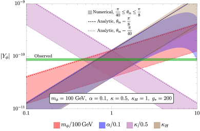
Figure 1: Analytic and numerical results for $|Y_{\phi}|$. The fiducial parameters are shown at the bottom of the plot, and the colored lines and bands show the case where one of the parameters is varied. We show analytic results in Eq. (10) for $\theta_{\textrm{in}}=\pi/8$ (dashed line) and $\theta_{\textrm{in}}=\pi/40$ (dotted line), and numerical results (bands) for $\theta_{\textrm{in}}$ values between them. $\theta_{\textrm{in}}=\pi/8$ corresponds to the maximum $Y_{\phi}$, while $\theta_{\textrm{in}}=\pi/40$ is the minimum within $10\%$ tuning. Note that the observed asymmetry value is shown in the green band and the labels of the horizontal axis for different colors are shown below the plot. See Supplemental Material for details.

Asymmetry transfer.—

The thermalization of $\phi$ with the SM thermal bath and the subsequent transfer of asymmetry to the SM sector take place via the neutrino portal. From Eq. (3), the relevant interactions are given by

$$\Delta{\cal L}=\bar{N}i\bar{\sigma}^{\mu}\partial_{\mu}N-\left(y_{\nu}\ell hN+\frac{1}{2}\lambda_{N}\phi NN+h.c.\right)\,.$$ (11)

Through the Yukawa coupling $y_{\nu}$, the RH neutrinos are produced from the SM thermal bath. The production of $N$ becomes cosmologically important when $\Gamma_{N}(T_{N})=H(T_{N})$, where

$$\Gamma_{N}\approx 4\times 10^{-3}y_{\nu}^{2}T\,$$ (12)

is the production rate of $N$ from the SM plasma Besak and Bodeker (2012); Garbrecht et al. (2013); Ghisoiu and Laine (2014). The neutrino Yukawa coupling can be written as $y_{\nu}=\sqrt{m_{N}m_{\nu}}/v$ for the RH neutrino mass $m_{N}$ in the vacuum. Thus, $T_{N}$ is given by Escudero and Witte (2020)

$$T_{N}\sim 5\,m_{N}\left(\frac{\sum m_{\nu}}{0.05\,{\rm eV}}\right).$$ (13)

If $T_{N}>T_{\rm AD}$, the population of $N$ leads to the thermal potential of $\phi$ as $\sim\lambda_{N}^{2}T^{2}|\phi|^{2}$ that spoils the Affleck-Dine mechanism. However, we can easily control the thermal effect by taking a relatively small neutrino Yukawa coupling. For $m_{N}\ll\sqrt{m_{\phi}M_{P}}\sim 10^{\rm 10}\,{\rm GeV}$, we can safely ignore the effect of $N$ for the scalar potential of $\phi$.

During the thermalization, we can neglect the slight change of the entropy density $s$ from new degrees of freedom in the thermal bath. Before the onset of asymmetry generation, the radial component of $\phi$ is positioned at the potential minimum given by Eq. (8). During this phase, the energy density of $\phi$ is dominated by the homogeneous kinetic energy and is given by $\rho_{\phi}\sim H^{3}M_{P}$. Thus, it is negligible in comparison to the radiation energy density, $\rho_{\textrm{rad}}\sim H^{2}M_{P}^{2}$. After the asymmetry generation, $\rho_{\phi}$ scales as $a^{-4}$ shortly during free-rolling and as $a^{-3}$ after it starts to oscillate near the origin. Although $\rho_{\phi}$ decreases slower than $\rho_{\textrm{rad}}\propto a^{-4}$, $\rho_{\phi}$ remains negligible compared to $\rho_{\textrm{rad}}$ until they get thermalized.

As the temperature becomes lower than $T_{N}$, $\phi$ and $N$ are all thermalized with the SM bath through the $\lambda_{N}\phi NN$ term, and asymmetry of $\phi$ is distributed to the SM lepton sector. The baryon asymmetry is also generated through the weak sphaleron process when the neutrino-portal interaction is in equilibrium before the electroweak phase transition ($T_{\rm EW}\approx 159\mathrm{\;GeV}$), more precisely before the freeze-out of the sphaleron process ($T_{\rm sp}\approx 132\mathrm{\;GeV}$) D’Onofrio et al. (2014). This translates to the lower bound on the RH neutrino mass as $m_{N}\gtrsim 26\mathrm{\;GeV}$. The bound on $m_{N}=\lambda_{N}\langle\phi\rangle_{T=0}$ in the simplest model of neutrino implies that the neutrino mass is Majorana type, i.e. the $B-L$ number should be spontaneously broken in the vacuum. The spontaneous breaking of $U(1)_{B-L}$ in the early Universe should not lead to a wash-out of the existing asymmetry.

After all AD sector particles decay, the asymmetry of the AD sector is evenly distributed to leptons and baryons due to the sphaleron process. Because $\phi$ carries $B-L$ charge $-2$, the final baryon asymmetry will have the same magnitude and opposite sign as the initial $\phi$ asymmetry Eq. (10), i.e. $Y_{B}=-Y_{\phi}$.

Majoron phenomenology—

The model has two SM singlet scalar fields: $\phi$ and $\tilde{N}$, where $\tilde{N}$ is the superpartner of $N$. The scalar dynamics at high temperatures is mostly dominated by $\phi$, while $\tilde{N}$ plays an important role at low temperatures. Our simple assumption is that $\tilde{N}$ has a tachyonic soft mass, which is set to be the electroweak scale for the same reason that $m_{\phi}$ is the electroweak scale. Then, the scalar potential from Eq. (3) for $\tilde{N}$ at low energy is

$$\Delta V= \,(\lambda_{N}^{2}|\phi|^{2}\hskip-1.42271pt-\hskip-1.42271ptm_{\tilde{N}}^{2})|\tilde{N}|^{2}+\left(\frac{\alpha\lambda_{N}m_{\phi}}{2}\phi\tilde{N}^{2}+h.c.\right)$$

$$+\frac{\lambda_{N}^{2}}{4}|\tilde{N}|^{4}+{\cal O}\left(\frac{\alpha m_{\phi}}{M_{P}}\tilde{N}^{4}\right),$$ (14)

where the last term is interactions suppressed by $M_{P}$ and is not relevant for scalar dynamics. At high temperatures $T>T_{\rm AD}$, $\tilde{N}$ is trapped at the origin because of a large positive mass contribution from $\lambda_{N}^{2}|\phi|^{2}\sim HM_{P}$. After the $Y_{\phi}$ generation, $\phi$ rolls to the origin with the behavior of $|\phi|^{2}\propto a^{-3}$. Because of the negative mass squared of $\tilde{N}$, $|\tilde{N}|$ gradually develops a nonzero expectation value as $\lambda_{N}^{2}|\phi|^{2}$ becomes smaller than $m_{\tilde{N}}^{2}$. Thereafter, the asymmetry of $\phi$ smoothly transfers to that of $\tilde{N}=\frac{1}{\sqrt{2}}r_{N}e^{i\theta_{N}}$. The dynamics of $\tilde{N}$ conserves the $B-L$ number, and the net density of the AD sector

$$\bar{n}_{B-L}|_{\rm AD}=-2\bar{n}_{\phi}+\bar{n}_{N}=-2r_{\phi}^{2}\dot{\theta}_{\phi}+r_{N}^{2}\dot{\theta}_{N}\equiv f_{J}^{2}\dot{\theta}_{J}$$ (15)

is decreasing as $a^{-3}$ until the explicit breaking effect becomes important. The $U(1)_{B-L}$ spontaneous breaking scale $f_{J}=\sqrt{4r_{\phi}^{2}+r_{N}^{2}}$ is gradually dominated by $r_{N}$. The associated Nambu-Goldstone boson, Majoron, corresponds to $J(x)=f_{J}\theta_{J}(x)$, and the $B-L$ asymmetry is carried by the kinetic energy of $J$ Chikashige et al. (1981); Gelmini and Roncadelli (1981).

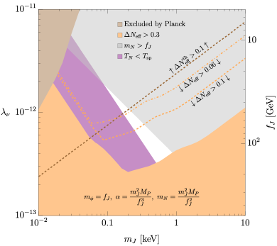
Figure 2: Constraints (shaded region) and future sensitivities (dashed and dot-dashed lines) in the $m_{J}-\lambda_{\nu}(f_{J})$ plane. The brown region is excluded by Planck Sandner et al. (2023), and the orange region is excluded from $\Delta N_{\textrm{eff}}>0.3$ Aghanim et al. (2020). The constraint $T_{N}>T_{\rm sp}$ (purple region) gives the upper bound on $f_{J}$, while the perturbativity condition for $\lambda_{N}$ (gray region) gives the lower bound. The allowed parameter space (white region) is near $f_{J}=\mathcal{O}(100\mathrm{\;GeV})$ and $m_{J}=\mathcal{O}(0.1-1\mathrm{\;keV})$, which are predicted values by the model. The dashed and dot-dashed lines are future sensitivities for $\Delta N_{\textrm{eff}}>0.1$ and $\Delta N_{\textrm{eff}}>0.06$, respectively. $\Delta N_{\textrm{eff}}^{\textrm{th}}$ indicates the contribution from the thermal production, while $\Delta N_{\textrm{eff}}$ denotes the contribution from the relic Majoron. Note all the allowed parameter space can be probed with the sensitivity $\Delta N_{\textrm{eff}}<0.06$.

The explicit breaking term of the scalar potential provides a damping effect. First of all, it gives a scalar potential for Majoron as $V_{J}\sim m_{J}^{2}f_{J}^{2}\cos(J/f_{J})$, where

$$m_{J}\sim f_{J}\sqrt{\frac{\alpha m_{\phi}}{M_{P}}}={\cal O}(0.1-1\mathrm{\;keV})\,.$$ (16)

We note that $\dot{\theta}_{J}$ remains much larger than $m_{J}$ when the AD sector is thermalized with the SM sector, which makes the damping effect negligible so the total $B-L$ number is nearly conserved. For $T_{\rm sp}\lesssim T\lesssim T_{N}$, the thermal potential for $r_{\phi}$ and $r_{N}$ could lead to the trap of the scalar fields at the origin $\langle f_{J}\rangle=0$ depending on the size of their thermal mass of ${\cal O}(\lambda_{N}T)$. After the sphaleoron process freezes out, $Y_{B}$ is entirely frozen.

Eventually, $U(1)_{B-L}$ is spontaneously broken with the vacuum expectation values

$$\langle|\phi|\rangle\sim\frac{\alpha m_{\phi}}{\lambda_{N}}~{}~{}\textrm{and}$$ (17)

$$\langle|\tilde{N}|\rangle\sim f_{J}\sim\frac{m_{\phi}}{\lambda_{N}}\,,$$ (18)

assuming $m_{\tilde{N}}\sim m_{\phi}$ and $\alpha\lesssim 1$. The Majorons are copiously produced around the $B-L$ phase transition and their density easily becomes an equilibrium value Li and Yu (2023). The Majoron decays after BBN and contributes to

$$\Delta N_{\textrm{eff}} = \frac{4}{7}\left(\frac{11}{4}\frac{g_{*S}(T_{0})}{g_{*S}(T_{d})}\right)^{4/3}\textrm{Max}\left[1,~{}\frac{30\zeta(3)}{\pi^{4}}\left(\frac{g_{*S}(T_{0})}{g_{*S}(T_{d})}\right)^{-1/3}\frac{m_{J}}{T_{\textrm{decay}}}\right]\,,$$ (19)

where $T_{0}$ is the temperature today, $T_{d}\sim 0.1m_{N}$ is the the temperature at Majoron decoupling Escudero and Witte (2021), and $T_{\textrm{decay}}$ is the temperature at Majoron decay. See Supplemental Material for details. If $f_{J}$ is excessively large, the Majoron decays much later than when it becomes non-relativistic. Since the energy density of non-relativistic particles redshifts slower than radiation, it contributes more to $N_{\rm eff}$ after decay, as shown in Eq. (19). The $N_{\rm eff}$ bound, $\Delta N_{\textrm{eff}}<0.3$ ($2\sigma$) from Aghanim et al. (2020), constrains $f_{J}$ not to significantly exceed the electroweak scale.

In Fig. 2, we show the constrained parameter space along with future $\Delta N_{\rm eff}$ sensitivities in the plane of $m_{J}$ and $\lambda_{\nu}(f_{J})$, where $\lambda_{\nu}\approx 0.05\mathrm{\;eV}/f_{J}$ is the Majoron-neutrino coupling. We have used $\mathcal{O}(1)$ model parameters to get $m_{J}$ and $f_{J}$ from the model parameters as shown in the plot, so note it can be modified by $\mathcal{O}(1)$ for different parameter choices. The orange region and lines come from the $\Delta N_{\textrm{eff}}$ contribution from the relic Majoron, while the brown region and line are from the late-time production from $J\leftrightarrow\nu\nu$. We require $T_{N}>T_{\rm sp}$, otherwise no baryon asymmetry is generated since thermalization of $N$ happens after the weak sphaleron process ceases. $m_{N}<f_{J}$ is imposed because the RH neutrino mass $m_{N}=\lambda_{N}\langle|\phi|\rangle$ needs to be smaller than the Majoron decay constant $f_{J}>\langle|\phi|\rangle$ with $\lambda_{N}<{\cal O}(1)$. The allowed parameter space nearly points $f_{J}={\cal O}(100\mathrm{\;GeV})$ and $m_{J}={\cal O}(0.1-1\mathrm{\;keV})$, which can be well predicted by our scenario. The future CMB observations for $\Delta N_{\rm eff}$ from Simons Observatory Ade et al. (2019) or CMB-S4 Abazajian et al. (2016) can probe all the allowed parameter space.

Discussion.—

The neutrino-portal Affleck-Dine mechanism yields the observed small baryon asymmetry in the Universe as a direct consequence of a hierarchy between two mass parameters inherent in the scenario, $m_{\phi}$ and $M_{P}$. Both parameters are linked to the symmetry-breaking scales and provide an organizing principle of the scalar potential. $M_{P}$ emerges as a cutoff scale in higher-dimensional operators that break global symmetries due to the quantum gravity effects. On the other hand, $m_{\phi}$ represents the soft supersymmetry breaking scale, which is the energy scale beyond which the potential of a scalar field remains shielded against UV-sensitive quantum corrections. This naturally prompts the exploration of the correlation between $m_{\phi}$ and the electroweak scale $v$.

An interesting relation between $m_{\phi}$ and $v$ arises in phenomenological observables as well. As shown in Fig. 2, the phenomenologically allowed values for the Majoron decay constant $f_{J}$, hence also for $m_{\phi}$, are close to the electroweak scale. This result is independent of the theoretical motivation for linking $m_{\phi}$ to $v$. Our scenario establishes a fundamental correlation between the electroweak scale and the origin of asymmetry in the Universe.

In contrast to conventional high-scale baryogenesis models, which typically do not predict any observable for new physics, our model has distinct low-energy observable implications in cosmology, yet asymmetry is still generated at a high scale, $T_{\rm AD}\sim 10^{10}\mathrm{\;GeV}$. The presence of a light Majoron with a keV mass is well predicted in the model, and the consequential effects on $N_{\rm eff}$ can be measured in the near future.

The reheating temperature needs to be higher than $T_{\rm AD}$ for the AD mechanism to work, but it cannot be significantly higher for two reasons. Firstly, a higher reheating temperature leads to a larger baryon isocurvature perturbation induced by a light field, the angular component of $\phi$ in this case, during inflation Akrami et al. (2020). Secondly, the scalar field $\phi$ undergoes negative damping at temperatures above $T_{\rm AD}$ if it is displaced from the fixed point Dine et al. (1996); Harigaya et al. (2015). The AD mechanism occurring shortly after reheating successfully exhibits all the previously discussed properties without these issues.

Our minimal scenario with SUSY has another phenomenological observable, which is that the lightest neutrino is almost massless, $m_{\rm light}\sim(m_{N}/M_{P})\sum m_{\nu}$. The future observations of the upper bound on neutrino masses from various experiments Amendola et al. (2018); Aghamousa et al. (2016) may provide a strong hint of the model. The more detailed connection to the spectrum of superpartners of the SM particles is also an important question, and it requires a more dedicated study of the SUSY-breaking mediation mechanism that will be revealed from the future observation of SUSY particles Workman et al. (2022); Allanach and Haber (2024). We leave this aspect to future works because all other aspects presented in this work yield consistent results as long as the same scalar potentials are employed. Here, SUSY only serves as a tool for organizing the scalar potentials.

Supplemental Material

I Scalar potential with softly broken supersymmetry

Supersymmetry (SUSY) is a generalization of the spacetime symmetries relating fermions and bosons. Because SUSY guarantees that quadratic divergences of all orders will cancel out in perturbation theory, the scalar potential can be well organized without worrying about various quantum corrections from UV physics. The supersymmetric Lagrangian can be systematically derived with the concept of superspace and superfield Salam and Strathdee (1974). Superspace is the coordinate space $(x,\theta,\bar{\theta})$ that contains anticommuting coordinates $\theta_{\alpha}$, $\bar{\theta}_{\dot{\alpha}}$ ($\alpha=1,2$) in addition to the usual spacetime coordinate $x$. Superfield is a field defined on superspace that is valued in a supermultiplet, an irreducible representation of the SUSY algebra. This contains both fermion and boson. The relevant superfield in our discussion is a chiral superfield, which can be written as

$$\Phi_{i}(y,\theta)=\phi_{i}(y)+\sqrt{2}\theta\psi_{i}(y)+\theta^{2}F_{i}(y)$$ (S1)

for $y=x+i\theta\sigma^{\mu}\bar{\theta}$. $\phi_{i}$ is a complex scalar, and $\psi_{i}$ is a chiral fermion, where $\phi_{i}$ and $\psi_{i}$ are superpartners of each other. $F_{i}$ is the auxiliary field whose nonzero expectation value contributes to the spontaneous breaking of SUSY.

The supersymmetric model of these fields $\phi_{i}$ and $\psi_{i}$ can be constructed as follows. For a given superpotential $W(\phi)$ (a holomorphic function of $\phi_{i}$),

$$W(\phi) =\mu_{ij}\phi_{i}\phi_{j}+\lambda_{ijk}\phi_{i}\phi_{j}\phi_{k}+\frac{\kappa_{ijkl}}{M_{P}}\phi_{i}\phi_{j}\phi_{k}\phi_{l}+\cdots$$ (S2)

and the Kähler potential $K(\phi,\phi^{\dagger})$ (a real-valued function of $\phi_{i}$ and $\phi_{i}^{*}$),

$$K(\phi,\phi^{\dagger}) =\phi_{i}^{\dagger}\phi_{i}+\frac{\kappa_{ij}}{M_{P}^{2}}\phi_{i}^{\dagger}\phi_{i}\phi_{j}^{\dagger}\phi_{j}+\cdots,$$ (S3)

the supersymmetric Lagrangian is given by

$${\cal L}_{\rm susy} =\int d^{2}\theta d^{2}\bar{\theta}\,K(\Phi,\Phi^{\dagger})+\int d^{2}\theta\,W(\Phi)+\int d^{2}\bar{\theta}\,\overline{W}(\Phi^{\dagger})$$

$$=K_{i\bar{j}}\left(\partial_{\mu}\phi_{i}\partial^{\mu}\phi^{*}_{j}+\frac{i}{2}D_{\mu}\psi_{i}\sigma^{\mu}\bar{\psi}_{j}-\frac{i}{2}\psi^{i}D_{\mu}\bar{\psi}_{j}\right)$$ (S4)

$$\quad-(K^{-1})_{\bar{i}j}\overline{W}_{i}W_{j}-\frac{1}{2}W_{ij}\psi_{i}\psi_{j}-\frac{1}{2}\overline{W}_{ij}\bar{\psi}_{i}\bar{\psi}_{j}+{\cal O}\left(\frac{\partial^{3}K}{\partial\phi_{i}\partial\phi_{j}\partial\phi^{*}_{k}}\right),$$ (S5)

where $\theta^{2}=\epsilon^{\alpha\beta}\theta_{\beta}\theta_{\alpha}$, $\bar{\theta}^{2}=\epsilon^{\dot{\alpha}\dot{\beta}}\bar{\theta}_{\dot{\alpha}}\bar{\theta}_{\dot{\beta}}$ and

$$W_{i} =\frac{\partial W(\phi)}{\partial\phi_{i}}=(\overline{W}_{i})^{*},\quad W_{ij}=\frac{\partial^{2}W(\phi)}{\partial\phi_{i}\partial\phi_{j}}=(\overline{W}_{ij})^{*},$$

$$K_{i\bar{j}} =\frac{\partial^{2}K(\phi,\phi^{\dagger})}{\partial\phi_{i}\partial\phi_{j}^{*}},\quad K_{i\bar{j}}(K^{-1})_{\bar{j}k}=(K^{-1})_{\bar{i}j}K_{j\bar{k}}=\delta_{ik}.$$ (S6)

The metric of the kinetic term is given by $K_{i\bar{j}}\simeq\delta_{ij}$, so the supersymmetric part of the scalar potential becomes

$$V_{\rm susy}\simeq\sum_{i}\left|\frac{\partial W}{\partial\phi_{i}}\right|^{2}.$$ (S7)

The higher order term in $K_{i\bar{j}}$ provides the interactions between the scalar fields and the kinetic terms as Eq. (6).

Besides the supersymmetric part, the scalar potential also contains the SUSY-breaking part as the result of the spontaneous breaking of SUSY. When SUSY is spontaneously broken, its effect must not lead to quadratic divergences in scalar masses. Such a class of supersymmetry breaking is called Soft SUSY breaking Dimopoulos and Georgi (1981). A phenomenological approach that takes these effects into account is to decompose the sectors into the visible sector which includes the AD sector ($\Phi$), the SUSY-breaking sector ($X$), and the messengers between them Martin (1998). For the discussion about the dynamics of the visible sector in the SUSY breaking background, we do not need to know the detailed mechanism of SUSY breaking. Its effect can be simply parameterized by the SUSY breaking spurion superfield

$$X=\theta^{2}F_{X},$$ (S8)

with a nonzero expectation value of $F_{X}$. The interaction between the SUSY breaking sector and the visible sector is mediated by some interactions suppressed by the messenger scale $M$ ($10\,{\rm TeV}\lesssim M\lesssim M_{P}$). For some reason, if the visible sector is completely decoupled from the SUSY breaking sector, it implies $M\to\infty$.

The interactions between $X$ and the visible sector fields at scales well below $M$ can be written as

$$\Delta W_{\rm soft} =\frac{1}{M}X\left(\alpha W(\Phi)+\alpha_{i}\Phi_{i}\frac{\partial W}{\partial\Phi_{i}}+\cdots\right),$$ (S9)

$$\Delta K_{\rm soft} =\frac{1}{M^{2}}X^{\dagger}X\left(\kappa_{i}\Phi_{i}^{\dagger}\Phi_{i}+\cdots\right).$$ (S10)

The overall soft SUSY breaking mass scale in the visible sector is parameterized by

$$m=\frac{F_{X}}{M}.$$ (S11)

The messenger scale $M$ and the size of dimensionless couplings are determined by the detailed mediation mechanism. However, it is natural that the overall mass scale $m$ is universal if the SUSY breaking terms originate from the same mediation mechanism. The corresponding soft SUSY breaking potential is

$$\Delta V_{\rm soft}=-\sum_{i}\kappa_{i}m^{2}|\phi_{i}|^{2}-\left(\alpha mW(\phi)+\sum_{i}\alpha_{i}m\,\phi_{i}\frac{\partial W}{\partial\phi_{i}}+h.c.\right)$$ (S12)

that provides contributions of Eqs. (5) and (Majoron phenomenology—).

II Calculations of $Y_{\phi}$

We provide more detailed explanations for the parameter dependence of $Y_{\phi}$ expressed in Eq. (10). The value of $Y_{\phi}(t)$ can be obtained by integrating the equation of motion of $n_{\phi}$ in Eq. (9) over $t$ with the potential Eq. (Asymmetry generation.—) and the initial condition $Y_{\phi}(t_{\rm in})=0$ in the radiation-dominated era:

$$Y_{\phi}(t) = -\int_{t_{\rm in}}^{t}\frac{1}{s}\frac{\partial V}{\partial\theta_{\phi}}dt^{\prime}$$ (S13)

$$= -\frac{1}{4}\left(\frac{90}{\pi^{2}g_{*}}\right)^{1/4}\left(\frac{\kappa\alpha m_{\phi}}{2M_{P}}\right)\int_{t_{\rm in}}^{t}\frac{r_{\phi}^{4}(t^{\prime})\sin{4\theta_{\phi}(t^{\prime})}}{(H(t^{\prime})M_{P})^{3/2}}\,dt^{\prime}\,.$$ (S14)

For the generation of asymmetry, the relevant dynamics arises when $H(t)=\frac{1}{2t}\sim m_{\phi}$, so we define $t_{*}$ with $H(t_{*})=m_{\phi}$ and rewrite Eq. (S14) with a dimensionless time variable $\tilde{t}=t/t_{*}$,

$$\tilde{Y}_{\phi}(\tilde{t})\equiv Y_{\phi}(t=\tilde{t}\,t_{*}) =-\frac{1}{6}\left(\frac{90}{\pi^{2}g_{*}}\right)^{1/4}\left(\alpha\frac{\kappa_{H}}{\kappa}\sin{4\theta_{\rm in}}\right)\sqrt{\frac{m_{\phi}}{M_{P}}}\int_{\tilde{t}_{\text{in}}}^{\tilde{t}}\frac{\tilde{t}^{\prime 3/2}}{2}\frac{\tilde{r}_{\phi}^{4}(\tilde{t}^{\prime})\sin{4\tilde{\theta}_{\phi}(\tilde{t}^{\prime})}}{r_{*}^{4}\sin{4\theta_{\rm in}}}\,d\tilde{t}^{\prime}\,.$$ (S15)

Here, $r_{*}=\langle r_{\phi}\rangle$ in Eq. (8) with $H=m_{\phi}$, $\tilde{t}_{\rm in}=t_{\rm in}/t_{*}$, and $\tilde{r}_{\phi}(\tilde{t})$ and $\tilde{\theta}_{\phi}(\tilde{t})$ are $r_{\phi}(\tilde{t}\,t_{*})$ and $\theta_{\phi}(\tilde{t}\,t_{*})$, respectively.

One can perform a numerical calculation for the integration part, but we can start with analytic calculations with several approximations. The radial and angular fields show different characteristics before and after the rolling of the fields. For $\tilde{t}\ll 1$, the angular field is frozen, and the radial field follows Eq. (8), which gives $r_{\phi}(t)\propto t^{-1/2}$, so we get $\tilde{r}_{\phi}^{4}(\tilde{t})\sin 4\tilde{\theta}_{\phi}(\tilde{t})/(r_{*}^{4}\sin 4\theta_{\rm in})\approx\tilde{t}^{-2}$. On the other hand, for $\tilde{t}\gg 1$, the real and imaginary parts of the complex scalar field $\phi$ are oscillating as the independent harmonic oscillators with the angular frequency $m_{\phi}$. At the same time, the average value of $r_{\phi}(t)$ decreases as $a^{-3/2}\propto t^{-3/4}$, therefore $r_{\phi}(t)\propto t^{-3/4}\cos{m_{\phi}t}$. The initial eccentricity is close to the unity so $\theta_{\phi}(t)$ remains $\theta_{\rm in}$ near the maximum of the oscillations. Thus we get $\tilde{r}_{\phi}^{4}(\tilde{t})\sin 4\tilde{\theta}_{\phi}(\tilde{t})/(r_{*}^{4}\sin 4\theta_{\rm in})\simeq\tilde{t}^{-3}(\cos\frac{1}{2}(\tilde{t}-1))^{4}$ for $\tilde{t}\gg 1$. Then the final $Y_{\phi}$ at $t\rightarrow\infty$ can be separated and analyzed as

$$Y_{\phi} \approx -\frac{1}{6}\left(\frac{90}{\pi^{2}g_{*}}\right)^{1/4}\left(\alpha\frac{\kappa_{H}}{\kappa}\sin{4\theta_{\textrm{in}}}\right)\sqrt{\frac{m_{\phi}}{M_{P}}}\left(\int_{0}^{1}\frac{1}{2\tilde{t}^{1/2}}\,d\tilde{t}+\int_{1}^{\infty}\frac{(\cos{\frac{1}{2}(\tilde{t}-1)})^{4}}{2\tilde{t}^{3/2}}\,d\tilde{t}\right)$$

$$\approx -\frac{1}{6}\left(\frac{90}{\pi^{2}g_{*}}\right)^{1/4}\left(\alpha\frac{\kappa_{H}}{\kappa}\sin{4\theta_{\rm in}}\right)\sqrt{\frac{m_{\phi}}{M_{P}}}\Big{(}1+0.48\Big{)}$$

$$\approx -0.1\,\alpha\frac{\kappa_{H}}{\kappa}\sin{4\theta_{\rm in}}\left(\frac{200}{g_{*}(T_{AD})}\right)^{1/4}\sqrt{\frac{m_{\phi}}{M_{P}}}\,,$$

where the integration range of is simplified to $(0,\infty)$ because the initial and final time values are far from $\tilde{t}=1$.

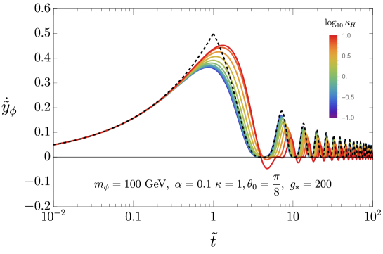
Figure S1: The $\kappa_{H}$-dependence of $\dot{\tilde{y}}_{\phi}(\tilde{t})$ defined by Eq. (S19) in radiation dominated era. The black dashed line is the analytic approximation given by Eq. (II) that shows a good agreement with the actual value from the solution of $\phi(t)$ to Eq. (S17) with a small deviation around $\tilde{t}=1$. This is true for other values of $\kappa_{H}$.

The numerical value of $Y_{\phi}$ is obtained from the following process. From the Eq. (Asymmetry generation.—), the equation of $\phi(t)$ is

$$\ddot{\phi}+3H\dot{\phi}+(m_{\phi}^{2}-\kappa_{H}H^{2})\phi-\frac{\kappa\alpha m_{\phi}}{M_{P}}\phi^{*3}+\frac{3\kappa^{2}}{M_{P}^{2}}\phi^{3}\phi^{*2}=0\,.$$ (S17)

Then, we can evaluate Eq. (S14) with

$$r_{\phi}^{4}\sin{4\theta_{\phi}}=-2i(\phi^{4}-\phi^{*4})$$ (S18)

for the numerical solution of $Y_{\phi}(t)$. Fig. S1 shows analytic and numerical evolutions of

$$\dot{\tilde{y}}_{\phi}(\tilde{t})\equiv\frac{\tilde{t}^{5/2}}{2}\frac{\tilde{r}_{\phi}^{4}(\tilde{t})\sin{4\tilde{\theta}_{\phi}(\tilde{t})}}{r_{*}^{4}\sin{4\theta_{\rm in}}}\approx\frac{d}{d\ln{\tilde{t}}}\left(\frac{\tilde{Y}_{\phi}(\tilde{t})}{\tilde{Y}_{\phi}(\tilde{t}=1)}\right)\,.$$ (S19)

The black dashed line represents the analytic approximation given by Eq. (II) and colored real lines are numerical values with the solution of $\phi(t)$. Here, we note that the quadratic potential of $r_{\phi}(t)$ changes its sign at $t=t_{\rm flip}$, where $\kappa_{H}H^{2}(t_{\rm flip})=m_{\phi}^{2}$. Depending on the size of $\kappa_{H}$, $t_{\rm flip}$ is different from $t_{*}$, but we confirm that $t_{*}$, rather than $t_{\rm flip}$, is the time when the behavior of $Y_{\phi}$ changes significantly, as shown in Fig. S1. We also display the final analytical and numerical results for $Y_{\phi}$ in Fig. 1, which shows how well the parameter-dependence of $Y_{\phi}$ in the analytical expression agrees with the numerical results.

III Late-time Evolution of Majorons

The Majoron emerges after the $B-L$ symmetry is spontaneously broken. Its mass in our scenario is ${\cal O}(0.1-1)$ keV, which is much smaller than all $B-L$ charged particles except the active neutrinos. The efficient way to write the relevant Lagrangian for Majoron cosmology is to take a field basis of heavy particles $\Phi_{i}$ (except the active neutrinos $\nu$) as

$$\Phi_{i}\to\Phi_{i}\exp(iq_{\Phi_{i}}\theta_{J})\,,$$ (S20)

where $q_{\Phi_{i}}$ is the $B-L$ charge of $\Phi_{i}$. Then, only the Majoron and active neutrinos are transformed as

$$U(1)_{B-L}:\quad\theta_{J}\to\theta_{J}+c,\quad\nu_{i}\to e^{-ic}\nu_{i}.$$ (S21)

After integrating out these massive fields, the relevant effective Lagrangian for the Majoron becomes

$${\cal L}_{\rm eff} =\frac{1}{2}f_{J}^{2}(\partial_{\mu}\theta_{J})^{2}-\left(\frac{1}{2}(m_{\nu})_{ij}e^{2i\theta_{J}}\nu_{i}\nu_{j}+h.c.\right)$$

$$\quad-\frac{\alpha m}{16M_{P}}\Big{(}\kappa\langle r_{\phi}^{4}\rangle e^{-8i\theta_{J}}+\kappa_{2}\langle r_{\phi}^{3}r_{N}\rangle e^{-5i\theta_{J}}+\kappa_{3}\langle r_{\phi}^{2}r_{N}^{2}\rangle e^{-2i\theta_{J}}+\kappa_{4}\langle r_{\phi}r_{N}^{3}\rangle e^{i\theta_{J}}+\kappa_{5}\langle r_{N}^{4}\rangle e^{4i\theta_{J}}+h.c.\Big{)}$$ (S22)

$$=\frac{1}{2}(\partial_{\mu}J)^{2}-\frac{1}{2}m_{J}^{2}J^{2}-J\left(\frac{i(m_{\nu})_{ij}}{f_{J}}\nu_{i}\nu_{j}+h.c.\right)+\cdots,$$

where $r_{\phi}=\sqrt{2}|\phi|$, $r_{N}=\sqrt{2}|\tilde{N}|$, the Majoron decay constant $f_{J}=\sqrt{\sum_{i}2q_{\Phi_{i}}^{2}\langle|\Phi_{i}|^{2}\rangle}=\sqrt{4\langle r_{\phi}^{2}\rangle+\langle r_{N}^{2}\rangle}$, and the canonically normalized Majoron $J(x)=f_{J}\theta_{J}(x)$. There are several contributions to the Majoron mass from the explicit $B-L$ breaking terms in the superpotential suppressed by $1/M_{P}$. Although the correct form of the Majoron mass is quite complicated and includes many parameters, we can easily identify its order of magnitude as $m_{J}^{2}\sim(\alpha m/M_{P})f_{J}^{2}$.

In our scenario, the Majoron $J$ is thermally produced after $B-L$ phase transition and its abundance is frozen at $T_{d}\sim 0.1m_{N}$, where $m_{N}$ is the right-handed neutrino mass and $T_{d}$ is the freeze-out temperature of the Majoron. Then relativistic Majoron contribution to $\Delta N_{\textrm{eff}}$ today is given by

$$\Delta N_{\textrm{eff}} = \frac{4}{7}\left(\frac{11}{4}\frac{g_{*S}(T_{0})}{g_{*S}(T_{d})}\right)^{4/3}\,.$$ (S23)

Since the Majoron mass is much smaller than $m_{N}$, the initial Majorons are relativistic. If the Majoron becomes non-relativistic before it decays away, an additional factor $F_{\rm NR}$ should be included as matter redshifts slower than radiation,

$$F_{\rm NR} = \int\frac{d^{3}p}{(2\pi)^{3}}\frac{m_{J}}{\exp{(p/T_{J,\textrm{decay}})}-1}\bigg{/}\int\frac{d^{3}p}{(2\pi)^{3}}\frac{p}{\exp{(p/T_{J,\textrm{decay}})-1}}$$ (S24)

$$= \frac{30\zeta(3)}{\pi^{4}}\left(\frac{g_{*S}(T_{0})}{g_{*S}(T_{d})}\right)^{-1/3}\frac{m_{J}}{T_{\textrm{decay}}}\,,$$ (S25)

where $T_{J,\textrm{decay}}$ and $T_{\textrm{decay}}$ are the temperatures of the Majoron and the photon, respectively, at which the Majoron decays. The rate of Majoron decay to neutrinos $\Gamma_{J}$ is Akita and Niibo (2023)

$$\Gamma_{J} = \frac{m_{J}}{16\pi f_{J}^{2}}\sum m_{\nu}^{2}$$ (S26)

$$\approx \frac{1}{3.3\times 10^{8}~{}\textrm{second}}\left(\frac{m_{J}}{1\mathrm{\;keV}}\right)\left(\frac{100\mathrm{\;GeV}}{f_{J}}\right)^{2}\left(\frac{\sum m_{\nu}^{2}}{10^{-3}\mathrm{\;eV}^{2}}\right)\,.$$ (S27)

By using $\Gamma_{J}=H$, we get

$$T_{\textrm{decay}}\approx 141\mathrm{\;eV}\left(\frac{m_{J}}{1\mathrm{\;keV}}\right)^{1/2}\left(\frac{100\mathrm{\;GeV}}{f_{J}}\right)\left(\frac{\sum m_{\nu}^{2}}{(0.05\mathrm{\;eV})^{2}}\right)^{1/2}\,,$$ (S28)

assuming the decay happens in the radiation-dominated era. The final contribution to $\Delta N_{\textrm{eff}}$ is given by

$$\Delta N_{\textrm{eff}} = \frac{4}{7}\left(\frac{11}{4}\frac{g_{*S}(T_{0})}{g_{*S}(T_{d})}\right)^{4/3}\textrm{Max}[1,F_{\rm NR}]$$ (S29)

$$\approx \begin{cases}0.029~{}\left(\frac{100}{g_{*S}(T_{d})}\right)^{4/3}&,~{}F_{\rm NR}\leq 1\\ 0.23~{}\left(\frac{m_{J}}{1\mathrm{\;keV}}\right)^{1/2}\left(\frac{f_{J}}{100\mathrm{\;GeV}}\right)\left(\frac{(0.05\mathrm{\;eV})^{2}}{\sum m_{i}^{2}}\right)^{1/2}\left(\frac{100}{g_{*S}(T_{d})}\right)&,~{}F_{\rm NR}>1\end{cases}$$ (S30)

References

- Aghanim et al. (2020) N. Aghanim et al. (Planck), Astron. Astrophys. 641, A6 (2020), [Erratum: Astron.Astrophys. 652, C4 (2021)], arXiv:1807.06209 [astro-ph.CO] .
- Bodeker and Buchmuller (2021) D. Bodeker and W. Buchmuller, Rev. Mod. Phys. 93, 035004 (2021), arXiv:2009.07294 [hep-ph] .
- Elor et al. (2022) G. Elor et al., in Snowmass 2021 (2022) arXiv:2203.05010 [hep-ph] .
- Barrow et al. (2022) J. L. Barrow et al., (2022), arXiv:2203.07059 [hep-ph] .
- Affleck and Dine (1985) I. Affleck and M. Dine, Nucl. Phys. B 249, 361 (1985).
- Dine et al. (1996) M. Dine, L. Randall, and S. D. Thomas, Nucl. Phys. B 458, 291 (1996), arXiv:hep-ph/9507453 .
- Allahverdi and Mazumdar (2012) R. Allahverdi and A. Mazumdar, New J. Phys. 14, 125013 (2012).
- sus (2000) The Supersymmetric World—The Beginnings of the Theory (World Scientific, Singapore, 2000) edited by G. Kane and M. Shifman, contains an early history of supersymmetry and a guide to the original literature.
- Ellis et al. (1984) J. R. Ellis, J. S. Hagelin, D. V. Nanopoulos, K. A. Olive, and M. Srednicki, Particle physics and cosmology: Dark matter, Nucl. Phys. B238, 453 (1984).
- Nilles et al. (1983) H. P. Nilles, M. Srednicki, and D. Wyler, Phys. Lett. 120B, 346 (1983).
- Minkowski (1977) P. Minkowski, Phys. Lett. B 67, 421 (1977).
- Ramond (1979) P. Ramond, in International Symposium on Fundamentals of Quantum Theory and Quantum Field Theory (1979) arXiv:hep-ph/9809459 .
- Gell-Mann et al. (1979) M. Gell-Mann, P. Ramond, and R. Slansky, Conf. Proc. C 790927, 315 (1979), arXiv:1306.4669 [hep-th] .
- Yanagida (1979) T. Yanagida, Conf. Proc. C 7902131, 95 (1979).
- Mohapatra and Senjanovic (1981) R. N. Mohapatra and G. Senjanovic, Phys. Rev. D 23, 165 (1981).
- Holman et al. (1992) R. Holman, S. D. H. Hsu, T. W. Kephart, E. W. Kolb, R. Watkins, and L. M. Widrow, Phys. Lett. B 282, 132 (1992), arXiv:hep-ph/9203206 .
- Kamionkowski and March-Russell (1992) M. Kamionkowski and J. March-Russell, Phys. Lett. B 282, 137 (1992), arXiv:hep-th/9202003 .
- Barr and Seckel (1992) S. M. Barr and D. Seckel, Phys. Rev. D 46, 539 (1992).
- Witten (1981) E. Witten, Nucl. Phys. B188, 513 (1981).
- Dimopoulos and Georgi (1981) S. Dimopoulos and H. Georgi, Nucl. Phys. B193, 150 (1981).
- Susskind (1984) L. Susskind, Phys. Rept. 104, 181 (1984).
- Girardello and Grisaru (1982) L. Girardello and M. T. Grisaru, Nucl. Phys. B194, 65 (1982).
- Hall and Randall (1990) L. J. Hall and L. Randall, Phys. Rev. Lett. 65, 2939 (1990).
- Kawasaki and Takesako (2012) M. Kawasaki and T. Takesako, Phys. Lett. B 711, 173 (2012), arXiv:1112.5823 [hep-ph] .
- Besak and Bodeker (2012) D. Besak and D. Bodeker, JCAP 03, 029 (2012), arXiv:1202.1288 [hep-ph] .
- Garbrecht et al. (2013) B. Garbrecht, F. Glowna, and P. Schwaller, Nucl. Phys. B 877, 1 (2013), arXiv:1303.5498 [hep-ph] .
- Ghisoiu and Laine (2014) I. Ghisoiu and M. Laine, JCAP 12, 032 (2014), arXiv:1411.1765 [hep-ph] .
- Escudero and Witte (2020) M. Escudero and S. J. Witte, Eur. Phys. J. C 80, 294 (2020), arXiv:1909.04044 [astro-ph.CO] .
- D’Onofrio et al. (2014) M. D’Onofrio, K. Rummukainen, and A. Tranberg, Phys. Rev. Lett. 113, 141602 (2014), arXiv:1404.3565 [hep-ph] .
- Chikashige et al. (1981) Y. Chikashige, R. N. Mohapatra, and R. D. Peccei, Phys. Lett. B 98, 265 (1981).
- Gelmini and Roncadelli (1981) G. B. Gelmini and M. Roncadelli, Phys. Lett. B 99, 411 (1981).
- Sandner et al. (2023) S. Sandner, M. Escudero, and S. J. Witte, Eur. Phys. J. C 83, 709 (2023), arXiv:2305.01692 [hep-ph] .
- Li and Yu (2023) S.-P. Li and B. Yu, (2023), arXiv:2310.13492 [hep-ph] .
- Escudero and Witte (2021) M. Escudero and S. J. Witte, Eur. Phys. J. C 81, 515 (2021), arXiv:2103.03249 [hep-ph] .
- Ade et al. (2019) P. Ade et al. (Simons Observatory), JCAP 02, 056 (2019), arXiv:1808.07445 [astro-ph.CO] .
- Abazajian et al. (2016) K. N. Abazajian et al. (CMB-S4), (2016), arXiv:1610.02743 [astro-ph.CO] .
- Akrami et al. (2020) Y. Akrami et al. (Planck), Astron. Astrophys. 641, A10 (2020), arXiv:1807.06211 [astro-ph.CO] .
- Harigaya et al. (2015) K. Harigaya, M. Ibe, M. Kawasaki, and T. T. Yanagida, JCAP 11, 003 (2015), arXiv:1507.00119 [hep-ph] .
- Amendola et al. (2018) L. Amendola et al., Living Rev. Rel. 21, 2 (2018), arXiv:1606.00180 [astro-ph.CO] .
- Aghamousa et al. (2016) A. Aghamousa et al. (DESI), (2016), arXiv:1611.00036 [astro-ph.IM] .
- Workman et al. (2022) R. L. Workman et al. (Particle Data Group), PTEP 2022, 083C01 (2022).
- Allanach and Haber (2024) B. Allanach and H. E. Haber, (2024), arXiv:2401.03827 [hep-ph] .
- Salam and Strathdee (1974) A. Salam and J. A. Strathdee, Nucl. Phys. B76, 477 (1974).
- Martin (1998) S. P. Martin, Adv. Ser. Direct. High Energy Phys. 18, 1 (1998), arXiv:hep-ph/9709356 .
- Akita and Niibo (2023) K. Akita and M. Niibo, JHEP 07, 132 (2023), arXiv:2304.04430 [hep-ph] .