Is GN-z11 powered by a super-Eddington massive black hole?

Abstract

Context. Observations of $z\sim 6$ quasars powered by super-massive black holes (SMBHs, $M_{\rm BH}\sim 10^{8-10}\,M_{\odot}$) challenge our current understanding of early black hole formation and evolution. The advent of the James Webb Space Telescope (JWST) has enabled the study of massive black holes (MBHs, $M_{\rm BH}\sim 10^{6-7}\ \mathrm{M}_{\odot}$) up to $z\sim 11$, thus bridging the properties of $z\sim 6$ quasars to their ancestors.

Aims. JWST spectroscopic observations of GN-z11, a well-known $z=10.6$ star forming galaxy, have been interpreted with the presence of a super-Eddington (Eddington ratio $\equiv\,\lambda_{\rm Edd}\sim 5.5$) accreting MBH. To test this hypothesis we use a zoom-in cosmological simulation of galaxy formation and BH co-evolution.

Methods. We first test the simulation results against the observed probability distribution function (PDF) of $\lambda_{\rm Edd}$ found in $z\sim 6$ quasars. Then, we select in the simulation those BHs that satisfy the following criteria: (a) $10<z<11$, (b) $M_{\rm BH}>10^{6}\ \mathrm{M}_{\odot}$. We then apply the Extreme Value Statistics to the PDF of $\lambda_{\rm Edd}$ resulting from the simulation.

Results. We find that the probability to observe a $z\sim 10-11$ MBH, accreting with $\lambda_{\rm Edd}\sim 5.5$, in the volume surveyed by JWST, is very low ($<0.5\%$). We compare our predictions with those in the literature and we further discuss the main limitations of our work.

Conclusions. Our simulation cannot explain the JWST observations of GN-z11. This might be due to (i) missing physics in simulations, or (ii) uncertainties in the data analysis.

1 Introduction

Observations show that the most distant quasars known so far (redshift $z=6-7.5$; see a recent review by Fan et al., 2023) are powered by SMBHs with masses $\sim 10^{8-10}\leavevmode\nobreak\ \rm M_{\odot}$ (e.g. Bañados et al., 2018; Yang et al., 2020; Wang et al., 2021; Farina et al., 2022; Mazzucchelli et al., 2023; Yang et al., 2023). The existence of these gigantic Black Holes (BHs) is a puzzle for current theoretical models of BH formation and evolution that is still lacking several pieces, e.g. knowledge about the SMBH seed nature and mass, and their ability to grow fast enough to assemble a SMBH in less than 1 Gyr, the age of the Universe at $z\sim 6$. Studying massive black holes (MBHs) of $\sim 10^{6-7}\mathrm{M}_{\odot}$ at redshift $z>9$ is essential to make a step forward in this field (Inayoshi et al., 2020; Volonteri & Bellovary, 2012). The recent claim of a vigorously accreting MBH in GN-z11, a well-known star forming galaxy at $z=10.6$ (Maiolino et al., 2023b), goes in such a direction.

GN-z11 was first identified by Bouwens et al. (2010) and Oesch et al. (2016), and recently followed up in the JWST Advanced Deep Extragalactic Survey (JADES, Eisenstein et al., 2023) by means of NIRSpec spectroscopy (Bunker et al., 2023) and NIRCam imaging (Tacchella et al., 2023). These observations suggest that GN-z11 is an Active Galactic Nuclei( AGN), with several evidences in favour of this interpretation (Maiolino et al., 2023b): (i) high ionization transitions (e.g. [NeIV]$\lambda 2422,2244$), which are commonly observed in AGNs (Terao et al., 2022; Le Fèvre et al., 2019) and are considered as tracers of AGN activity since they require high photon energies ($E_{\rm\nu}>63.5\ \mathrm{eV})$ that are not easily produced by stars; (ii) $\mathrm{NIII}]$ multiplet, indicating gas densities $(>10^{10}\ \rm cm^{-3})$ typically found in the Broad Line Regions (BLRs) of AGN; (iii) a very deep equivalent width $(\mathrm{EW_{rest}\sim 5\AA})$ and blueshifted absorption trough of CIV doublet, suggesting the presence of outflows with velocities ($\sim 800-1000\ \mathrm{km\ s^{-1}}$) commonly observed in mini-Broad Absorption Line (BAL) quasars (Rodríguez Hidalgo, 2009); (iv) clear detection of MgII doublet hinting at the presence of an accreting MBH with mass $\sim 1.2\times 10^{6}\ \mathrm{M}_{\odot}$ and a surprisingly large Eddington ratio ($\lambda_{\rm Edd}=L_{\rm bol}/L_{\rm Edd}\sim 5.5\pm 2$).

The high accretion rate of GN-z11 provides important constraints for theoretical models predicting the mass and the formation epoch of early SMBH seeds (Inayoshi et al., 2020; Volonteri et al., 2021; Latif & Ferrara, 2016). The various possibilities include: (1) light seeds ($\sim$10^1-2 $\rm M_{\odot}$) from Pop III stars (z$\sim$20-30, Madau & Rees, 2001); (2) intermediate seeds ($\sim$10^3-4 $\rm M_{\odot}$) from the collapse of supermassive stars or runaway collisions in dense, nuclear star clusters; (z$\sim$10-20, Devecchi et al., 2012; Greene et al., 2020) (3) heavy seeds ($\sim$10^5-6 $\rm M_{\odot}$) produced by the collapse of metal-free gas in atomic-cooling (virial temperature $T_{vir}>10^{4}$ K) halos exposed to a strong Lyman-Werner radiation (z$\sim$10-20), the so-called direct collapse black holes (DCBHs, Ferrara et al., 2014; Haehnelt & Rees, 1993; Mayer & Bonoli, 2019).

Which of the above scenarios is the most favourable to explain the existence of SMBHs at high-$z$ is still unclear. On the one hand, the DCBH scenario has the advantage that heavy seeds can grow at a mild pace, namely at sub-Eddington rates ($f_{\rm Edd}=\dot{M}/\dot{M}_{\rm Edd}<1$). However, the conditions for the formation of DCBH are not easily satisfied. On the other hand, light/intermediate seeds can form in less extreme circumstances, but require sustained ($f_{\rm Edd}>1$) accretion rates for prolonged ($\sim\rm Gyr$) intervals of time.

Semi-analytical works that support light seeds scenarios are based on radiatively-inefficient ”slim disk” models in which super/hyper Eddington accretion (Sadowski, 2009) can occur (e.g. Madau et al., 2014; Pezzulli et al., 2016, 2017). However, it is still not completely understood how much these results depend on the assumptions adopted. To start with, Madau et al. (2014) assume that, in super/hyper Eddington accretion regimes, gas can flow toward the center BH almost non-affected by feedback processes. However, radiative feedback in radiatively-efficient ”thin disk” models (e.g. Pacucci & Ferrara, 2015; Orofino et al., 2018) has been shown to modify the accretion flow onto the BH both decreasing the accretion to sub-Eddington rates or making $f_{\rm Edd}>1$ episodes intermittent. In particular, Pacucci et al. (2017) have shown that very efficient and prolonged large accretion rates only occur in $M_{\rm BH}>10^{4}\leavevmode\nobreak\ M_{\odot}$. For what concerns the Pezzulli et al. (2017) results, the adoption of $f_{\rm Edd}>500$ values, which goes beyond the applicability of the adopted ”slim disk” recipe, may overestimate the accretion rate of light seeds, and therefore the final mass of the SMBH formed.

Hydro-dynamical simulations developed so far have provided further important information about this issue. Lupi et al. (2016) have produced high-resolution ($<1$pc) simulations of an isolated disk in which the radiatively inefficient supercritical accretion of light seeds occurs in the high density environment of gaseous circumnuclear disks. These authors find that 10-100 M_⊙ BHs can increase their mass within a few million years by one up to three orders of magnitudes, depending on the resolution adopted (the higher is the resolution the lower is the final mass of the grown seed). Less efficient growth of light seeds has been found by Smith et al. (2018) that have followed the evolution of Bondi accreting BHs from Pop III stars in high resolution cosmological simulations finding a much smaller ($<$10% of their initial mass) average mass increase. Similar conclusions have been drawn by a comprehensive study performed by Zhu et al. (2022) that have considered various recipes for BH seeding, accretion models and feedback processes. Even in the most optimistic conditions (radiatively inefficient, super Eddington accretion), and although spending a substantial fraction of time ($\sim 100$ Myr) in super-critical accretion, light seeds ($M<10^{3}\mathrm{M}_{\odot}$) cannot reproduce $>10^{7}\mathrm{M}_{\odot}$ ($>10^{5}\mathrm{M}_{\odot}$) BHs at $z\sim 6$ ($z\sim 11$).

Current investigations have thus not yet definitively clarified whether light seeds can provide a valuable route for the formation of high-$z$ massive black holes. Furthermore, high-resolution (computationally expensive) hydro-dynamical simulations are required to proper follow the growth of light seeds. Several works (see Table 1 in Habouzit et al., 2021) have thus opted for assuming the DCBH scenario as a seeding prescription. Here, we adopt the cosmological zoom-in hydrodynamical simulations developed by Valentini et al. (2021, hereafter V21). These simulations can reproduce the main properties of the most luminous $z\sim 6$ quasars (see Table 2 and 3 in V21), namely both mass of their central SMBHs ($\sim 10^{9}\leavevmode\nobreak\ \rm M_{\odot}$), suggested by observations of the CIV and MgII lines (e.g. Farina et al., 2022; Mazzucchelli et al., 2023), and high star formation rates (SFR$\sim 100\rm\leavevmode\nobreak\ M_{\odot}\leavevmode\nobreak\ yr^{-1}$), and large masses ($\sim 10^{9}\leavevmode\nobreak\ \rm M_{\odot}$) of molecular gas, suggested by ALMA observations (e.g. Wang et al., 2016; Venemans et al., 2017, 2020; Gallerani et al., 2017; Decarli et al., 2018, 2022). In this work we investigate the predictions of V21 simulations in terms of the accretion properties that characterise $z\sim 10-11$ BHs as massive as the one hosted in GN-z11 ($M_{\rm BH}\gtrsim 10^{6}\leavevmode\nobreak\ \rm M_{\odot}$).

In particular, to test whether the V21 simulations can reproduce the $\lambda_{\rm Edd}\sim 5.5$ found in GN-z11, we adopt the Extreme Value Statistics (EVS Gumbel, 1958; Kotz & Nadarajah, 2000). The EVS has been applied to a wide range of topics in cosmology (Lovell et al., 2023; Harrison & Coles, 2011; Colombi et al., 2011; Chongchitnan & Silk, 2012; Davis et al., 2011; Waizmann et al., 2011; Mikelsons et al., 2009; Chongchitnan & Silk, 2021) and can be used to calculate the probability of randomly extracting the largest (or smallest) value from an underlying distribution.

The Letter is organized as follows: in Sec.  2, we describe the adopted numerical simulations; we then compare the simulated Eddington ratio PDF with observations in Sec.  3. In Sec.  4 we compute the exact EVS PDF of Eddington ratio for GNz11-like MBH from the simulations. Finally, we discuss our results and draw our conclusions in Sec.  5.

2 Simulations

We use the hydrodynamical cosmological zoom-in simulations developed by Valentini et al. (2021, hereafter V21), and summarise below the main features of this model. In particular, we consider the AGN fiducial run featuring thermal AGN feedback as our fiducial model, and we refer to V21 for more details. The V21 simulation adopted in this work is performed with a non-public version of the TreePM (particle mesh) and SPH (Smoothed Particles Hydrodynamics) code GADGET-3 (Valentini et al., 2017, 2019, 2020), an evolved version of the public GADGET-2 code (Springel, 2005).

2.1 Initial conditions and resolution

The software MUSIC Hahn & Abel (2011) is used to generate the initial conditions, assuming a $\Lambda$CDM cosmology. First, a dark matter (DM)-only simulation with mass resolution of DM particles of $9.4\times 10^{8}\leavevmode\nobreak\ \mathrm{M}_{\odot}$ in a comoving volume of $(148\leavevmode\nobreak\ {\rm Mpc})^{3}$ is run starting from $z=100$ down to $z=6$. Then, a halo as massive as $M_{\rm halo}=1.12\times 10^{12}\leavevmode\nobreak\ \mathrm{M}_{\odot}$ at $z=6$ is selected for a zoom-in procedure, to run the full hydrodynamical simulation. In the zoom-in region, the highest resolution particles have a mass of $m_{\rm DM}=1.55\times 10^{6}\ \mathrm{M}_{\odot}$ and $m_{\rm gas}=2.89\times 10^{5}\ \mathrm{M}_{\odot}$. The gravitational softening lengths are$\epsilon_{\rm DM}=0.72$ ckpc and $\epsilon_{\rm bar}=0.41$ ckpc for DM and baryon particles, respectively.

2.2 Sub-resolution physics

2.2.1 Black hole seeding

DM halos exceeding the threshold mass $M_{\mathrm{DM}}=1.48\times 10^{9}\leavevmode\nobreak\ \mathrm{M}_{\odot}$ are seeded with a BH of mass $M_{\mathrm{BH,seed}}=1.48\times 10^{5}\leavevmode\nobreak\ \mathrm{M}_{\odot}$ if no BH was already seeded. This value of seed mass mimics the DCBH scenario.

2.2.2 Black hole growth

BHs grow due to gas accretion and merger with other BHs. The gas accretion is modeled assuming a Bondi–Hoyle–Lyttleton accretion solution (Bondi, 1952; Hoyle & Lyttleton, 1939; Bondi & Hoyle, 1944):

$$\dot{M}_{\rm bondi}=\frac{4\pi G^{2}M_{\rm BH}^{2}\langle\rho_{\rm gas}\rangle}{(\langle c_{\rm s}\rangle^{2}+\langle v_{\rm BH}\rangle^{2})^{3/2}},$$ (1)

where $M_{\rm BH}$ is the mass of the BH, $\rho_{gas}$ is the gas density, $G$ is the gravitational constant, $c_{s}$ is the sound speed, $v_{\rm BH}$ is the velocity of the BH relative to the gas. All the quantities of the gas particles are calculated within the BH smoothing length using kernel-weighted contributions. The BH accretion rate is capped to the Eddington value. A small fraction, $\epsilon_{r}\ \dot{M}_{\rm accr}$, of the accreted mass is converted in radiation; thus, the actual growth rate of the BH mass can be written as

$$\dot{M}_{\rm BH}=(1-\epsilon_{\rm r})\ \dot{M}_{\rm accr},$$ (2)

where $\epsilon_{r}$ =0.03 is the radiation efficiency (Sadowski & Gaspari, 2017). BHs instantaneously merged if their distance becomes smaller than twice their gravitational smoothing length, and if their relative velocity is smaller than 0.5 $c_{\rm s}$ ($v_{\rm BH-BH}<0.5\ \langle c_{\rm s}\rangle$). The position of the resulting BH will be the position of the most massive one between the two progenitor BHs.

2.2.3 AGN feedback

For what concerns AGN feedback, a fraction $\epsilon_{\rm f}=10^{-4}$ (V21) of the bolometric luminosity $L_{\rm bol}=\epsilon_{\rm r}\dot{M}_{\rm BH}c^{2}$ is distributed to the gas particles thermally and isotropically within the BH smoothing volume (Valentini et al., 2020).

3 Eddington ratio predictions against $z\sim 6$ data

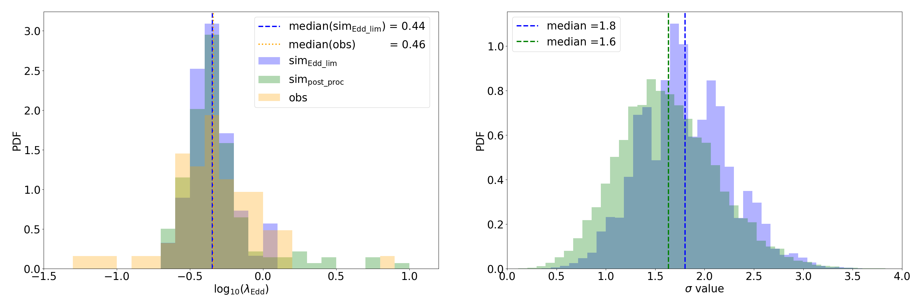
Figure 1: Left panel: Comparison between one realization of resampled (see Sec. 3) Eddington ratio values obtained from the Eddington-limited accretion model (V21; blue histogram), and in post-processing from V21 using Eq. 1 (green histogram). The distribution of Eddington ratio values measured from a literature sample of quasars at 6¡z¡7.5 is shown with an orange histogram. The orange (blue) vertical dotted (dashed) line shows the median of the observations (Eddington ratio values from the Eddington-limited accretion model by V21). Right panel: distribution of the $\sigma$ values obtained by applying the two sample K-S test on $N_{\rm re-samp}=10^{6}$ number of resamples. The blue (green) PDF refers to the $\sigma$ distribution corresponding to the original (post-processed) values of $\lambda_{\rm Edd}$ from the V21 simulation. The vertical blue and green dashed lines show the median of the blue and green distributions, respectively.

In this section, we compare the Eddington ratios $\lambda_{\rm Edd}$ measured for $z\sim 6-7.5$ quasars with the results from the V21 simulation. The Eddington ratio is defined as $\lambda_{\rm Edd}={L_{\rm bol}}/{L_{\rm Edd}}$, namely the ratio between the bolometric luminosity of a quasar and its Eddington luminosity that, under the assumption of hydrostatic equilibrium and pure ionized hydrogen, can be written as (Eddington, 1926):

$$L_{\rm Edd}=\frac{4\pi G\ M_{\rm BH}\ m_{\rm p}\ c}{\sigma_{\rm T}},$$ (3)

where $m_{\rm p}$ is the mass of a proton and $\sigma_{\rm T}$ is the Thomson scattering cross-section.

For what concerns the observed $\lambda_{\rm Edd}$ values, we consider both the sample of 38 quasars by Farina et al. (2022, hereafter F22) and 42 quasars by Mazzucchelli et al. (2023, hereafter M23), the latter including the XQR-30 sample of VLT-XSHOOTER observations (D’Odorico et al., 2023). Of the 80 quasars in the combined sample, 18 of them are present in both samples. In these cases, we consider the data which are characterised by the smallest error. After removing duplications, we end up with 62 bright quasars at 5.8 $<$ z $<$ 7.5. In the following we refer to these combined sample as the ”literature sample”.

F22 and M23 provide the $\lambda_{\rm Edd}$ values resulting from the analysis of the MgII and CIV emission lines, using different methods (MgII line: Vestergaard & Osmer 2009, Shen et al. 2011; CIV line: Vestergaard & Peterson 2006, Coatman et al. 2017). When the MgII line is available, we use the Shen et al. (2011) method, since it provides the smallest errors (see also Shen & Liu, 2012, for a comparison among different virial BH mass estimators); for those targets in which only the CIV line fit is provided, we adopt the Vestergaard & Peterson (2006) method. The resulting ”observed” PDF of the $\lambda_{\rm Edd}$ values is shown in the left panels of Fig. 1 through the orange shaded region.

To compute $\lambda_{\rm Edd}$ values from simulation, we consider the accretion rate of those SMBHs that have masses consistent with the literature sample (namely $M_{\rm BH}>10^{8}$ M_⊙) in the redshift range $6<z<7.5$. We end up with 2 SMBHs that satisfy these criteria. We finally select the SMBH with $L_{\rm bol}>2.7\times 10^{46}\ \mathrm{L}_{\odot}$. This choice enables a proper comparison between observations and simulation, since the observed sample consists of very luminous quasars (the least luminous source has $L_{\rm bol}=2.86^{+0.17}_{-0.15}\times 10^{46}\ \mathrm{L}_{\odot}$). We evaluate $\lambda_{\rm Edd}$ for the selected BH at each time-step of the simulation in the redshift range $6<z<7.5$. We consider each accretion episode as independent and compute the corresponding PDF. The resulting ”simulated” PDF is shown in the left panels of Fig. 1 with a blue shaded region.

From the comparison between the observed and simulated PDF it results that the median of these distributions (0.46 for the observed PDF and 0.44 for the simulated one) are perfectly consistent with each other (see the vertical orange and blue lines in the left panel of Fig. 1). We further apply the two-sample Kolmogorov–Smirnov (K-S) test (Kolmogorov, 1933; Smirnov, 1948) to the observed and simulated PDFs. We account for the uncertainties in the observed PDF by adopting the bootstrap re-sampling technique as in F22. To this aim, we first randomly re-sample the observed PDF $N_{\rm re-samp}$ times, taking into account the errors associated to the observational values. Then, we include the average error of the literature sample ($\sim 0.1\ \mathrm{dex}$, see Table 4 in F22 and Table 1 in M23) in the simulated PDF, and we randomly re-sample it as done for the observed one. Finally, for each $N_{\rm re-samp}$ couple, we perform the two sample K-S test and we associate the corresponding $\sigma$ values to the resulting p-values.

The right panel of Fig. 1 shows the PDF of the $\sigma$ values resulting from the bootstrap re-sampling technique considering $N_{\rm re-samp}=10^{6}$. The median of the $\sigma$ value PDF is 1.8. We find that the probability of having $\sigma$ values $>$3 is very small ($\sim$1%) implying that the probability of rejecting the null hypothesis that these two samples are drawn from the same underlying distribution is not significant. We can thus conclude that the simulated PDF provides a good representation of the observed one.

In the V21 simulation, however, the BH accretion is capped at the Eddington limit. To check whether and how much this assumption in the simulation is affecting the results, we use Eq. 1 to re-compute the accretion rate of the BHs for which $\lambda_{\rm Edd}=1$, and we repeat the K-S test analysis as detailed above. The results are shown in the right panel of Fig. 1 with a green shaded region. The new median of the $\sigma$ value PDF is 1.6 (instead of 1.8); the probability that we can reject the null hypothesis in this case is also $\sim$1%. This simple test suggests that our conclusions are not biased by the Eddington cap prescription on the accretion. We will further discuss this caveat in Sec. 5.

We finally compare the results of our simulation with the NIRSpec/PRISM sample by Greene et al. (2023) which contains 7 AGN with $L_{\rm bol}>10^{44.2}\rm erg/s$ within the redshift range $5.8<z<8.5$. For these sources, the estimated Eddington ratios range from 0.04 to 0.4. Such range is consistent with the mean $\lambda_{\rm Edd}$ value (0.14) found in our simulation, by applying the same luminosity cut in the redshift range $6<z<8.5$.

Table 1: Properties of host galaxy of the most massive BH in simulation at z=10 and GN-z11 (from Tacchella et al. (2023))

	SIM value	Observational value
log $M_{*}[\mathrm{M}_{\odot}]$	8.9	9.1${}^{+0.3}_{-0.4}$
SFR $[\mathrm{M}_{\odot}\leavevmode\nobreak\ \mathrm{yr}^{-1}]$	5.4	21${}^{+20}_{-10}$

4 Eddington ratio predictions against $z\sim 10$ data

Once that we have checked that the V21 model is able to reproduce the accretion properties of the well-studied population of $z\sim 6$ quasars, we search in the simulation for BHs with $M_{\rm BH}\sim 10^{6}\mathrm{M}_{\odot}$ in the redshift range $10<z<11$ to investigate whether the same model can reproduce the properties of GN-z11 at $z=10.6$. We find one BH-galaxy system in our simulated volume that can be representative of GN-z11. The BH, seeded at $z\sim 16.1$, has a mass of $=1.4\times 10^{6}\mathrm{M}_{\odot}$ at $z=10.6$, fairly consistent with the BH mass of GN-z11; however, it is accreting at $\lambda_{\rm Edd}=0.6$, that is smaller than what is suggested for GN-z11. We further report in Table 1 the properties of its host galaxy at $z=10$, namely at the closest snapshot in our simulation to the GN-z11 redshift. The galaxy properties are consistent (within 1.6-$\sigma$) with those of GN-z11, both in terms of stellar mass ($M_{*}$) and star formation rate (SFR), as computed by Tacchella et al. (2023).

Furthermore, we compute the $\lambda_{\rm Edd}$ distribution of our GN-z11-like AGN with the same procedure adopted in Sec. 3, and we report the results in Fig. 2 with a shaded blue region. It is still possible that GN-z11 has been detected while it was experiencing a rare episode of super-Eddington accretion. To compute the likelihood of this scenario we rely on the so-called Extreme Value Statistics (EVS), detailed in Appendix A.

4.1 EVS application to GN-z11

To apply the EVS to the case of GN-z11, we need to know both (i) the functional form describing the PDF and CDF ($f(x)$ and $F(x)$, respectively, in Eq. 6) of the simulated $\lambda_{\rm Edd}$ distribution, and (ii) the number of random extractions ($N$ in Eq. 6) that applies to the case of JWST observations.

For what concerns (i), we simply fit the blue shaded region in Fig. 2 with a Gaussian (solid blue line in Fig. 2) and we compute the corresponding CDF. When fitting the simulated PDF with a Gaussian (solid blue line), the tail extends beyond the Eddington cap. Thus, even if the V21 simulations are capped to the Eddington limit, the probability of having extreme events, such as super-Eddington accretion episodes, is non-vanishing.

The calculation of (ii) is instead less trivial. We associate the number $N$ of random extractions to the number of DM halos contained in the volume $V$ ($\sim 1.2\times 10^{6}\ \mathrm{Mpc}^{3}$) covered by the observations (Oesch et al., 2016) that discovered GN-z11 in the CANDELS field. We thus adopt the following relation:

$$N=V\int_{m1}^{m2}\ dM\ \left(\frac{dn(M)}{dM}\right)_{z=10.6},$$ (4)

where $m_{1}$ and $m_{2}$ represent the minimum and maximum mass of the DM halo that are expected to host GN-z11, and $\frac{dn(M)}{dM}$ is the halo mass function, for which we consider the Sheth & Tormen (1999) functional form. We assume $m_{2}=10^{13}\leavevmode\nobreak\ \rm M_{\odot}$ because we notice that larger values do not change our results, since the integral already converged with the assumed $m_{2}$ value. To estimate $m_{1}$, we adopt three different and independent approaches that rely on the SFR, $M_{*}$, and $M_{\rm BH}$ estimates of GN-z11 (see Appendix B). We derive that GN-z11 is hosted by a DM halo with a fiducial mass of $M_{\rm h}\sim 0.7-4\times 10^{11}\mathrm{M}_{\odot}$. However, values as small as $M_{\rm h}\sim 4\times 10^{9}\leavevmode\nobreak\ \rm M_{\odot}$ are not excluded by our analysis. We find $N=0.006$, for $m_{1}=4\times 10^{11}\mathrm{M}_{\odot}$ , namely no DM halos of this mass are expected to be in the survey volume. Hence, we consider $7\times 10^{10}\mathrm{M}_{\odot}$ as the largest value for $m_{1}$, and $4\times 10^{9}\mathrm{M}_{\odot}$ as the smallest one.

Fig. 2 shows the EVS for the above mentioned different values of $m_{1}$ (see also Table 2). For the smallest value of $m_{1}$, namely the one that is providing the largest number of DM haloes ($N=16416$), $P\left(\lambda_{\rm Edd}>1\right)=0.99$, and $P\left(\lambda_{\rm Edd}>3.5\right)=5\times 10^{-3}$. This means that our model allows for a non-vanishing probability of super-Eddington accretion episodes if $m_{1}=4\times 10^{9}\mathrm{M}_{\odot}$, but the probability of having $\lambda_{\rm Edd}$ values as large as the one observed in GN-z11 is very small in any case.

We have repeated the same calculation of the accretion rate for those few ($\sim 2\%$) $\lambda_{\rm Edd}=1$ episodes, by removing the Eddington cap. We find that the results reported in Table 2 do not change. The maximum value of the Eddington ratio obtained in this case is $\lambda_{\rm Edd}=2.24$. Such value is smaller than that reported in Maiolino et al. (2023b).

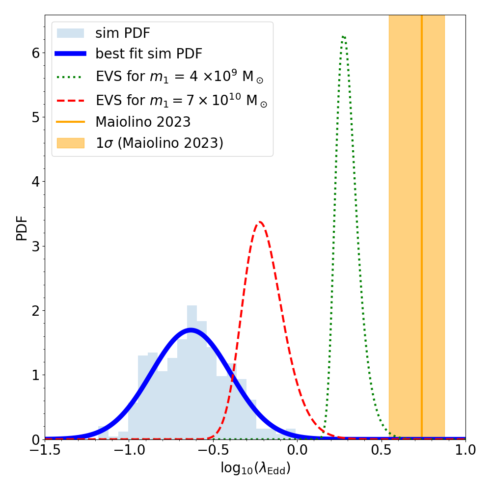
Figure 2: Extreme Value Statistics PDF as a function of the Eddington ratio for a GN-z11-like AGN. Blue solid line shows the best fit Gaussian to the Eddignton ratio distribution from the V21 simulation for BHs in the redshift range $10<z<11$ and $M_{\rm BH}>10^{6}M_{\odot}$. The dashed (dotted) red (green) line represents the EVS for the largest (smallest) considered value of $m_{1}$ (see text). The orange solid line (shaded region) shows the GN-z11 Eddington ratio (1$\sigma$ uncertainty) estimated by Maiolino et al. (2023b)

Table 2: EVS probability for $\lambda_{\rm Edd}>1$ and $>3.5$ (namely the 1$\sigma$ lower limit of the estimate by Maiolino et al. (2023b) for GN-z11), as resulting from different values of $m_{1}$ (see Eq. 4)

$m_{1}$[$\mathrm{M}_{\odot}$]	$N$	P($\lambda_{\rm Edd}$¿1)	P($\lambda_{\rm Edd}$¿3.5)
$4\times 10^{9}$	16416	0.99	$5\times 10^{-3}$
$7\times 10^{10}$	20	0.07	$6\times 10^{-6}$

5 SUMMARY & DISCUSSION

In this Letter, we have investigated the probability of having MBH ($\sim 10^{6}M_{\rm\odot}$) at $z\sim 10-11$ accreting at super-Eddington rate ($\lambda_{\rm Edd}\sim 5.5$), like the one recently detected by JWST in GN-z11 (Maiolino et al., 2023b).

We have first considered the accretion properties of simulated accreting SMBHs at $z\sim 6-7.5$ as provided by the zoom-in simulations developed by Valentini et al. (2021). By comparing the simulated $\lambda_{\rm Edd}$ probability distribution function (PDF) with the results from a state-of-the-art sample of $z\sim 6$ quasars (Farina et al., 2022; Mazzucchelli et al., 2023) we find that our accretion model successfully reproduces the data.

We have then analysed the $\lambda_{\rm Edd}$ PDF of MBHs at $z\sim 10-11$, and computed the extreme value statistics (EVS). By assuming that the observations that discovered GN-z11 are covering a $\sim 1.2\times 10^{6}\ \mathrm{Mpc}^{3}$ volume (Oesch et al., 2016), we find that the probability of finding a GN-z11-like object is very small ($\sim 10^{-3}$). However, our result does not exclude the presence of an MBH that is partly powering the GN-z11 luminosity.

A limitation of our work is that we are interpreting the super-Eddington accretion of GN-z11 with a model that caps the accretion to the Eddington limit. We justify this approximation with the fact that the V21 accretion model predicts that the probability of having maximal accretion ($\lambda_{Edd}=1$) is extremely small ($\sim 2\%$, see the blue distribution in Fig. 2). Thus, the assumption of the Eddington cap is affecting only a negligible number of accretion episodes. It is not straightforward to quantify the impact of the Eddington cap on the actual accretion rate. This is because feedback from super-Eddington episodes could highly affect the surrounding medium, possibly quenching subsequent accretion events. Such expectation is corroborated by the results in Massonneau et al. (2023, see Fig. 11 and 12). These authors have compared the accretion rate evolution of MBHs as predicted by simulations with and without super-Eddington accretion and feedback. They found that models that account for super-Eddington accretion result in a smaller fraction of Eddington accretion episodes compared to the Eddington-capped case. This means that if the Eddington cap would be removed in our simulation, the $\lambda_{Edd}$ PDF would shift towards smaller values, thus yielding an even smaller EVS probability for $\lambda_{Edd}>1$ .

If we consider the results of literature works allowing super-Eddington accretion rates onto BHs, the occurrence of $\lambda_{\rm Edd}\sim 5.5$ events is anyway unlikely. To start with, in Massonneau et al. (2023) super-Eddington accretion events reach peak values of only $2-3$ times the Eddington limit. Zhu et al. (2022) performed zoom-in hydrodynamical simulations of $z>6$ SMBHs exploring models with different seeding prescriptions, radiative efficiencies, accretion and feedback models. In these simulations, the most extreme accretion event for MBHs is characterised by $\lambda_{\rm Edd}=2.6$ and it only occurs at $z<10$. Furthermore, in the radiation-hydrodynamics study by Pacucci & Ferrara (2015), the average Eddington ratio of the considered MBH is $\lambda_{\rm Edd}\sim 1.35$. The accretion halts when the emitted luminosity reaches the value $\sim 3L_{\rm Edd}$. Finally, even state-of-the-art simulations (Lupi et al., 2023) cannot explain the observational results of GN-z11, since super-Eddington accretion events (up to $\lambda_{\rm Edd}\sim 10-100$, in this case) onto a $10^{6}\leavevmode\nobreak\ \rm M_{\odot}$ BH only occurs at $z<9.5$.

Another caveat is that we have used results from a single zoom-in simulation. This is clearly insufficient to perform an extensive statistical analysis of the problem. In fact, when comparing the observed $\lambda_{\rm Edd}$ distribution with simulation, we are considering a simulated massive black hole evolving from $10^{8}\mathrm{M}_{\odot}$ at $z=7.5$ to $10^{9}\mathrm{M}_{\odot}$ at $z=6$. In other words, we are making the strong assumption of associating different observed quasars to an accreting SMBH captured at different times during its accretion history.

Another assumption in our model that may affect the final results of our work concerns the seeding recipe. We have in fact considered only the possibility that SMBH can originate from heavy-seeds (seed mass $\sim 10^{5}\mathrm{M}_{\odot}$). It is not straightforward to foresee how this assumption might affect the simulated $\lambda_{\rm Edd}$ PDF, and corresponding EVS. We can however mention that models considering the light seed scenario and allowing for super-Eddington accretion are unlikely to explain the extreme $\lambda_{\rm Edd}$ value found in GNz-11. For example, Smith et al. (2018) post-processed the Renaissance simulation to follow the growth of BHs from individual remnants of Pop III stars finding that (i) for the majority of the $\sim 15000$ BHs the accretion rate was very small ($<10^{-4}\ \lambda_{\rm Edd}$); (ii) only a small fraction $(2-3\%)$ of BHs accreted with $\lambda_{\rm Edd}>10^{-4}$; (iii) only one BH accreted at maximum with $\lambda_{\rm Edd}\sim 3$, once.

The robustness of the main conclusion of our work, namely the low probability of having a $10^{6}\leavevmode\nobreak\ \rm M_{\odot}$ super-Eddington accreting BH at $z\sim 10$, is weakened by the assumptions discussed above and the limitations of our approach. Still, our model proposes a novel method to link JWST observations with theoretical models to interpret, in particular, the over-abundance of AGN found at high-$z$ (e.g. Maiolino et al., 2023a; Harikane et al., 2023).

The most promising way to overcome the limitations of our work is to apply the EVS method to multiple large scale simulations (e.g. Habouzit et al., 2021, 2022) which consider different seeding prescriptions that also include light and intermediate seeds (Zhu et al., 2022). Furthermore, for a fair comparison with observed super-Eddington accretion events it is important to properly model super-Eddington accretion in simulations adopting the radiatively inefficient ”slim disk” solution (Sadowski, 2009). In this case, in fact, there is not a linear relation between $\lambda_{\rm Edd}$ and $\dot{M}_{\rm BH}/\dot{M}_{\rm Edd}$; in particular, the measured value of $\lambda_{\rm Edd}$ is expected to plateau at $\sim 3$ for $\dot{M}_{\rm BH}/M_{\rm Edd}>10$ (Madau et al., 2014).

From the observational point of view, further detections and characterization of sources similar to GN-z11 in the early Universe will be fundamental to better constrain theoretical models and test their predictions against a larger data sample.

Appendix A The Extreme Value Statistics

Let us consider a cumulative distribution function (CDF), $F(x)$, and let us draw a sequence of N random variates $\left\{X_{i}\right\}$ from it. Let us call $X_{max}\equiv{\rm sup}\left\{X_{1}...X_{N}\right\}$ the largest value of this sequence. If all variables are identically distributed and mutually independent then the probability that all of the deviates are less than, or equal to, some $x$ is given by:

$$\centering\begin{array}[]{cl}\Phi\left(X_{\rm max}\leq x;N\right)&=F_{1}\left(X_{1}\leq x\right)..F_{N}\left(X_{N}\leq x\right)\\ &=F^{N}(X).\\ \end{array}\@add@centering$$ (5)

The PDF of $X_{\rm max}$ can then be obtained by differentiating Eq. 5 with respect to $x$:

$$\centering\begin{array}[]{cl}\Phi\left(X_{\rm max}=x;N\right)&=N\ F^{\prime}(x)\left[F(x)\right]^{N-1}\\ &=N\ f(x)\left[F(x)\right]^{N-1},\end{array}\@add@centering$$ (6)

where $f(x)=dF(x)/dx$ is the PDF of the considered distribution. Eq. 6 provides the probability of finding the extreme value $X_{\rm max}$ after randomly extracting $N$ variables from a given distribution $f_{x}$.

Appendix B Halo mass estimation for GN-z11

In this Appendix, we compute the range of the allowed masses for the DM haloes that host GN-z11, based on the SFR and $M_{*}$ estimates, and considering different $M_{\rm BH}-M_{*}$ relations. We find that the fiducial value corresponds to $M_{\rm h}=4\times 10^{11}\leavevmode\nobreak\ \rm M_{\odot}$ .

B.1 Halo mass estimation from the SFR

To estimate the halo mass $M_{h}$ from the star formation rate SFR we adopt the relation proposed by Ferrara et al. (2023),

$$\mathrm{SFR}=22.7\ \left(\frac{\epsilon_{\rm SF}}{0.01}\right)\ \left(\frac{1+z}{8}\right)^{3/2}\ \left(\frac{M_{\rm h}}{10^{12}\ \mathrm{M}_{\odot}}\right)\ \mathrm{M}_{\odot}\ \mathrm{yr}^{-1}$$ (7)

where $\epsilon_{\rm SF}$ is star formation efficiency that depends on the supernova (SN) feedback as in Dayal et al. (2014):

$$\epsilon_{\rm SF}=\epsilon_{0}\ \frac{v_{c}^{2}}{v_{c}^{2}+f_{w}\ v_{s}^{2}},$$ (8)

where $f_{w}=0.1$ is the coupling efficiency of SN energy with gas, $v_{c}(M)$ is the halo circular velocity (e.g. Barkana & Loeb, 2001), $\epsilon_{0}$ is fixed to 0.02 to be consistent with local galaxy measurements (Krumholz, 2017), $v_{s}=\sqrt{\nu\ E_{0}}$ is the characteristic velocity corresponding to the SN energy ($E_{0}$) released per unit stellar mass. Considering $E_{0}=10^{51}\ \mathrm{erg}$ and $\nu^{-1}=52.89\ \mathrm{M}_{\odot}$ same as in Ferrara et al. (2023), we get $v_{s}=975\ \mathrm{km\ s^{-1}}$.

The SFR of GN-z11 derived from the NIRCam photometry (assuming no contribution from the AGN) is ${\rm SFR}=21^{+22}_{-10}\ \mathrm{M}_{\odot}\ \mathrm{yr}^{-1}$ (Tacchella et al., 2023). This corresponds to $M_{\rm h}=4\times 10^{11}\leavevmode\nobreak\ \rm M_{\odot}$. By considering the 2 $\sigma$ deviation, we end up with the following possible range of halo mass: $5\times 10^{10}<(M_{\rm h}/\mathrm{M}_{\odot})<1\times 10^{12}$.

B.2 Halo mass estimation from the stellar mass

The stellar mass $M_{*}$ can be related to the halo mass $M_{\rm h}$ using the following relation:

$$M_{\rm h}=\frac{\Omega_{\rm dm}}{\Omega_{\rm b}}\ \left(\frac{M_{*}}{\epsilon_{\rm*}}\right),$$ (9)

where $\epsilon_{\rm*}=0.1$ is the conversion efficiency of baryons to stars. The stellar mass of GN-z11 derived from the NIRCam photometry is $\mathrm{log}_{10}(M_{*}/\mathrm{M}_{\odot})=9.1^{+0.3}_{-0.4}$ (Tacchella et al., 2023). This corresponds to $M_{\rm h}=7\times 10^{10}\leavevmode\nobreak\ \rm M_{\odot}$. By considering the 3 $\sigma$ deviation, we end up with the following possible range of halo mass: $4\times 10^{9}<(M_{\rm h}/\mathrm{M}_{\odot})<5\times 10^{11}$.

B.3 Halo mass estimation from the BH mass

In the local Universe, the BH mass scales with the stellar mass as $M_{\rm BH}\sim 10^{-4}\leavevmode\nobreak\ M_{*}$ (Reines & Volonteri, 2015). However, it has been found that high-$z$ SMBHs can be overmassive with respect to their low-z counterparts by a factor $>\times$10 (Pensabene et al., 2020; Pacucci et al., 2023). In particular, Pacucci et al. (2023), suggest for the high-$z$ the following relation: $M_{\rm BH}\sim 10^{-2}\leavevmode\nobreak\ M_{*}$. By combining the local and high-$z$ relations with Eq. 9, and assuming $M_{\rm BH}=1.6\times 10^{6}\ \rm M_{\odot}$ (Maiolino et al., 2023b), we estimate that GN-z11 should be host by a DM halo of mass $9\times 10^{9}<(M_{\rm h}/\mathrm{M}_{\odot})<9\times 10^{11}$.