Kibble-Zurek mechanism and errors of gapped quantum phases

Abstract

Kibble-Zurek mechanism relates the domain of non-equilibrium dynamics with the critical properties at equilibrium. It establishes a power law connection between non-equilibrium defects quenched through a continuous phase transition and the quench rate via the scaling exponent. We present a novel numerical scheme to estimate the scaling exponent wherein the notion of defects is mapped to errors, previously introduced to quantify a variety of gapped quantum phases. To demonstrate the versatility of our method we conduct numerical experiments across a broad spectrum of spin-half models hosting local and symmetry protected topological order. Furthermore, an implementation of the quench dynamics featuring a topological phase transition on a digital quantum computer is proposed to quantify the associated criticality.

I Introduction

The exploration of quantum phases at absolute zero and transitions among them is a cornerstone of condensed matter physics. The classification of quantum phases is an active area of research, specially as the investigation extends beyond the principles of Landau symmetry breaking. Essentially, there is a comprehensive understanding of quantum phases characterized by local order, yet comprehending phases that go beyond local order poses significant challenges. The study of associated Quantum Phase Transitions (QPT) provides critical insight into the universal behavior linked to the divergence in the correlation length. This makes it possible to categorize phases in different universality classes being identified by a set of critical exponents.

Kibble-Zurek Mechanism (KZM) provides critical insight into the dynamics of a system driven through a continuous phase transition Kibble (1976, 1980); Zurek (1985, 1993). Introduced in the context of cosmological phase transitions, the importance of the KZM lies in its ability to elucidate the emergence of defects during rapid phase transitions Kibble (1976, 1980); Zurek (1985, 1993); del Campo and Zurek (2014) while establishing a relationship between non-equilibrium dynamics and the critical exponents associated with phase transitions. Lately, this mechanism has been extended to encompass quantum many-body systems Ebadi et al. (2021); Zurek et al. (2005); Dziarmaga (2005a); Cincio et al. (2007); Dziarmaga (2009); Damski et al. (2011); Puebla et al. (2019); Kolodrubetz et al. (2012); Gong et al. (2015); Chandran et al. (2012); Rams et al. (2019); Francuz et al. (2016); Schmitt et al. (2021); Dupont and Moore (2022), and referred to as Quantum Kibble-Zurek Mechansim (QKZM). QKZM describes the quantitative behaviour of the defects in situations where the rate of change of the Hamiltonian is faster than the inverse of the spectral gap of the underlying system. The quantity of defects evolving through a QPT can be measured by employing the critical properties linked to it. Specifically, the defect density follows a power-law relationship with the quench rate, introducing a parameter known as the scaling exponent $\mu$.

Recent advancements in the development of several quantum architectures has propelled significant interest in exploring various quantum many-body phenomena Smith et al. (2019); de Léséleuc et al. (2019); Brydges et al. (2019); Bhattacharyya et al. (2022); Wei et al. (2023). In particular, QKZM has been validated on different quantum hardware platforms by estimating the critical properties, especially in Ising-like models Keesling et al. (2019); Dupont and Moore (2022). Motivated by the recent progress, in this work, we introduce a novel numerical scheme to obtain the scaling exponent in QPTs that are in principle accessible on a quantum device. We emphasize that the introduced method is not limited to the scope of the Landau symmetry breaking principle, and can be applied to a broader range of QPTs involving phases characterized by non-local order. To this extent, we further present strategies that enable numerical and experimental observation of QKZM involving symmetry protected topological phases. This in turn can be used as a scheme to profile and benchmark the performance of quantum computing devices.

We structure the rest of paper as follows: in Sec. II, we briefly review a quench protocol that realizes the QKZM, followed by introducing expectation value based strategies to determine the defect densities. In addition, we describe various components involved in estimating the scaling exponent in the thermodynamic limit. In Sec. III, we start our numerical investigations by studying the transverse field Ising model that exhibits local order. In Sec. IV, we extend the analysis to study phase transitions involving symmetry protected topological phases by considering various model Hamiltonians. Further, in Sec. V, we present an experimental prototype that allows the estimation of the scaling exponent associated with a topological phase transition on a digital quantum computer. Towards the end, in Sec. VI, we summarize the main results while outlining some future directions that can be explored using the computational strategies and protocols introduced.

II Quench protocol, defect density and critical exponent

We start by presenting the quench protocol as in the context of QKZM while introducing methods to compute defect densities and to estimate the corresponding scaling exponent.

II.1 Revisiting the QKZM

The QKZM process relies on a quench dynamics that can be generated by a time-dependent Hamiltonian, $H(t)$, connecting point $I$ to $F$,

$$H(t)=H_{F}+g(t)H_{I},$$ (1)

with $g(t)=-t/\tau_{Q}$ where $t\in(-\infty,0]$, $\tau_{Q}$ being the rate of the quench del Campo and Zurek (2014). Having the system prepared in the groundstate of the Hamiltonian, $H_{I}$, we evolve the system under the total Hamiltonian mentioned in Eq. 1. Assuming that there exists a second-order QPT at some critical strength $g(t_{c})$, QKZM establishes a power law relation between the defect density, $\eta$, at the final time and the quench rate, $\tau_{Q}$. The resulting relation is expressed as $\eta\propto\tau_{Q}^{-\mu}$, where $\mu$ is the scaling exponent characterizing the universality of the underlying QPT  Zurek et al. (2005); Dziarmaga (2005b); Polkovnikov (2005).

To quantify the defects we propose numerical methods that are applicable over a wide range of quantum phases characterized by various local and non-local orders. To this extent, we introduce the notion of errors with respect to a reference state that have been used as a numerical probe to characterize topological orders Jamadagni and Weimer (2022a, b). In addition, these concepts have been employed in conjugation with machine learning techniques that further enhance the detection of various quantum phases  Jamadagni et al. (2023). In the current scenario, we note that the aforementioned errors can be interpreted as defects as in the context of QKZM. For the purpose of demonstrating the notion of errors with respect to a reference state, we assume the Hamiltonian, $H_{F}$ in Eq. 1 is gapped and refer to the groundstate of the Hamiltonian as the reference state. In a more general context, the reference state is given by the eigenstate of the operator corresponding to the order parameter that maximizes the same. The errors are defined by the action of local operators (local perturbation) on the reference state. In the following sections, we will explicitly introduce the errors associated with the choice of the corresponding Hamiltonian. We also note that in the rest of our description, we interchangeably use the terms defect (density) and error (density).

II.2 Methods to compute defect density

In the following, we introduce two different computational strategies that estimate the density of errors. Given a gapped Hamiltonian, we compute the above based on expectation values of certain projectors in an exact and an approximate fashion Han et al. (2018); Jamadagni and Weimer (2022b); Jamadagni et al. (2023).

Method 1: Expectation value of the projectors

Let us assume that the Hamiltonian, $H_{F}$, can be expressed as a sum of $k$-local Hamiltonians, $h_{i}$, as in Eq. 2,

$$H_{0}=\sum\limits_{i}h_{i}.$$ (2)

We denote the energy spectrum of the $k$-local Hamiltonian $h_{i}$ by $\lambda^{i}_{j}$ and the corresponding eigenstates by $\ket{\lambda^{i}_{j}}$ with the groundstate denoted by setting $j=0$. For any given state $\ket{\psi}$, the total number of local errors with respect to the reference state $\ket{\lambda^{i}_{0}}$ for the $k$-sites is given by $\eta_{i}$, as in the Eq. 3,

$$\eta_{i}=1-\braket{\mathcal{P}^{i}_{0}},$$ (3)

where $\mathcal{P}^{i}_{0}=\ket{\lambda_{0}^{i}}\bra{\lambda_{0}^{i}}$ (or in the case of degeneracy $\mathcal{P}^{i}_{0}=\sum\limits_{d}\ket{\lambda_{0d}^{i}}\bra{\lambda_{0d}^{i}}$ with $d$-degenerate groundstates). For $k$ sites, since $\sum\ket{\lambda^{i}_{0}}\bra{\lambda^{i}_{0}}=\mathds{1}$, and $\mathcal{P_{0}^{i}}$ projecting into the groundstate of the $k$-local Hamiltonian, results in the total number of local errors, $\eta_{i}$, as in Eq. 3. Finally, we arrive at the total defect density as the total number of defects averaged over the system size, i.e., $\eta=\sum_{i}\eta_{i}/N$.

Method 2: Monte-Carlo based sampling

The defect densities can be obtained by measuring the wavefunction in the error basis. Numerically, we simulate the above by employing the Monte-Carlo sampling. First, we compute the expectation values of the $k$-local projectors $\mathcal{P}_{0}^{i}$. Next, we generate a random number, $r$ and if $r<\braket{\mathcal{P}_{0}^{i}}$ we identify the $k$-sites with a no-error configuration and otherwise as an error. In the case of the erroneous configuration, we apply the projector $P_{0}^{i}$, else we apply $\mathds{1}-P_{0}^{i}$ and renormalize the wavefunction. We repeat the above strategy over all the remaining $k$-local Hamiltonians and capture the corresponding errors for a single trajectory. We obtain the defect densities by normalizing over the system size and averaging it over considerable number of trajectories.

We note that the above process is akin to simulating the measurement of a wavefunction in an experimental setup. However, in a real experiment it might not always be possible to engineer the $k$-local projector and further perform a mutli-site measurement. In order to circumvent the above complexity, in the later sections, we propose a model dependent $m$-local measurement operator with $m<k$ that captures (partial) information about errors at the same time being experimentally more accessible.

(a)

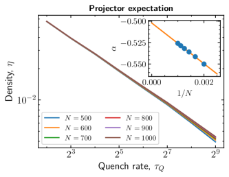
(b)

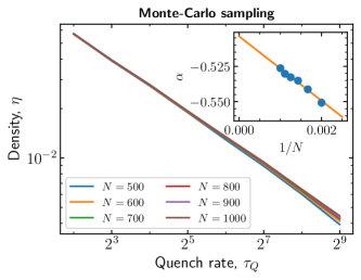
Figure 1: QKZM with the quench protocol driven across a paramagnetic-ferromagnetic QPT as in the tranverse field Ising model. Defect density, $\eta$, as a function of the quench rate, $\tau_{Q}$, with $\eta$ computed using the strategy based on (a) expectation value of the projector, (b) Monte-Carlo sampling. The linear scaling remains indistinguishable for progressively increasing values of $N$ indicating convergence to the behavior in the thermodynamic limit. We note that in the rest of the figures, we consider the y-axis on a decimal logarithm scale for better representation but the actual fit is made with respect to $\log_{2}$ on both axes. (Inset) By performing finite-size scaling analysis we estimate the critical exponent $\mu$ to be (a) 0.502(1), (b) 0.504(2) in the thermodynamic limit.

II.3 Extraction of the scaling exponent

Having defined two different strategies to compute the defect density, in the following, we outline a numerical procedure to determine scaling exponent, $\mu$ arising in the QKZM.

1. We set the initial time of the quench dynamics to be $t_{i}=\beta\tau_{Q}$, where $\beta$ is some constant such that $g(t_{i})\gg g(t_{c})$ with the final time of the dynamics as $t_{f}=0$, leading to $H_{I}$ being turned off. Next, we evolve the initial state through a QPT by employing the Hamiltonian in Eq. 1;

2. For different quench rates, we evolve the corresponding initial states. Following the above, we compute the error densities of the final evolved state;

3. For a given system size, we further extract $\mu$ by linearly fitting the defect density, $\eta$ with respect to the quench rate, $\tau_{Q}$, (on a $\log-\log$ scale i.e., $\log_{2}\eta\propto-\mu\log_{2}\tau_{Q}$). We then perform a finite-size scaling analysis to estimate the scaling exponent $\mu$ in the thermodynamic limit.

III Quantum phases with local order

To demonstrate the protocol, in this section, we consider a setting wherein a quantum phase characterized by local order is driven across criticality by a time-dependent perturbation. We begin by studying the paradigmatic model, the Transverse Field Ising Model (TFIM) that exhibits local order. The model consists of linear chain of $N$ spin-1/2’s with open boundary condition defined by the following Hamiltonian

$$H_{\text{TFIM}}(t)=-\sum\limits_{i=1}^{N-1}\sigma_{z}^{i}\sigma_{z}^{i+1}-g(t)\sum\limits_{j=1}^{N}\sigma_{x}^{j},$$ (4)

where the nearest neighbor interaction is ferromagnetic in nature with the strength of transverse field being time-dependent, $g(t)$, as defined previously in Eq. 1.

The above Hamiltonian exhibits a QPT with the groundstate being a paramagnet in the low perturbed regime while being a ferromagnet in the high perturbed regimes with a criticality at $g(-\tau_{Q})$=1. To estimate the critical exponent, we first choose the initial state to be the groundstate of Eq. 4 at some high field strength, thereby belonging to the paramagnetic phase. Then we evolve the system across the QPT guided by the quench protocol. In the current context, the reference state that leads to the construction of errors is the ferromagnetic groundstate i.e., $\ket{0000...00}$ and $\ket{1111...11}$. The presence of the transverse field gives rise to errors that are recognized by neighboring spins with opposite parity when measured in the $\sigma_{z}$ basis. Having introduced the quench dynamics and the errors associated with the ferromagnetic groundstate, we quantify the scaling exponent by employing the strategies as outlined in Sec. II.2.

III.0.1 Quantifying criticality using expectation value

As noted in Sec. II.2, the local defect density is captured by Eq. 3, which in the current scenario reduces to, $\mathcal{P}_{0}^{i}=\ket{00}\bra{00}_{(i,i+1)}+\ket{11}\bra{11}_{(i,i+1)}$. Equivalently, this can be represented as the expectation of the projector $\frac{\mathds{1}-\sigma_{z}^{i}\sigma_{z}^{i+1}}{2}$, that detects the presence of domain walls. The total error density is therefore given by

$$\eta=\frac{1}{N}\sum\limits_{i=1}^{N-1}\left(1-\braket{\ket{00}\bra{00}}_{(i,i+1)}-\braket{\ket{11}\bra{11}}_{(i,i+1)}\right).$$ (5)

To extract the exponent, $\mu$, for a given system size $N$, we deploy the procedure as outlined in Sec. II.3. In order to gain access to significantly higher system sizes we consider the Matrix Product State (MPS) representation of the quantum states in the rest of the analysis. The initial state i.e., the ground state is computed using the Density Matrix Renormalization Group (DMRG) algorithm and the time evolution is performed using the Time Evolution Block Decimation (TEBD) algorithm Vidal (2004) by choosing the Trotter scheme wherein the total error scales quadratically in the time step. We note that both the above implementations are realized by employing the ITensor library Fishman et al. (2022). From the numerical simulations, see Fig. 1, we obtain the critical exponent to be $\mu=0.502(1)$ that agrees well with the results obtained in Refs. Sachdev, 1999; Keesling et al., 2019. We note that the error can be further suppressed by choosing higher order Trotterization schemes.

III.0.2 Quantifying criticality using Monte-Carlo sampling

In the following, we employ the Monte-Carlo based sampling to obtain the errors using single-site measurements as in Ref. Jamadagni et al., 2023. That is, we sample the final evolved wavefunction in the $\sigma_{z}$ basis and identify the errors by the presence of different parity bits on the neighboring sites. In other words, the simulation of Monte-Carlo sampling generates the so called shot data as in the context of quantum computing. The tensor network based simulation in conjugation with the Monte-Carlo sampling leads to the critical exponent to be $\mu=0.504(2)$ which is in good agreement with the value obtained earlier. The projector, $\mathcal{P}_{0}^{i}$, in the TFIM is a diagonal operator and therefore is easier to access in an experimental setting. However, in the next sections, we explore systems that involve non-diagonal projection operators. Thereby, Monte-Carlo sampling techniques introduced here provide a means to estimate the defect density experimentally in a feasible manner.

IV Quantum phases with symmetry protected topological order

In this section, we extend the analysis to the context of topological phases, phases that are beyond the Landau symmetry breaking principle thereby being characterized by non-local order parameters. We restrict our analysis to topological phases hosting short-range entangled states with a given symmetry, also know as Symmetry Protected Topological (SPT) states. The short-range entanglement implies that they can smoothly deformed into a product state unless the deformation preserves the symmetry. In other words, SPT states cannot be mapped to a product state using finite-depth symmetry preserving local unitaries Chen et al. (2010). In the following, we consider three different time-dependent Hamiltonians that host SPT phases along with a quench protocol that drives these phases across a QPT. We further employ the computational methods introduced earlier to estimate the scaling exponent associated with the topological phase transition.

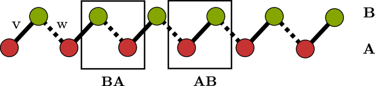
Figure 2: The SSH model describes the hopping of a particle between distinct neighboring sites A and B with alternating bond strengths $v$ and $w$ identified by the unit cells AB and BA. In the hardcore boson variant, we consider a half-filled lattice of $N$ sites with each unit cell hosting a single particle in the limits of $v=0$ and $w=0$. We note that when $v=0$ we observe $N/2$ dimerized unit cells while in the other limit $w=0$ we notice $N/2-1$ dimers in addition to unpaired edge sites giving rise to the so called edge modes.

(a)

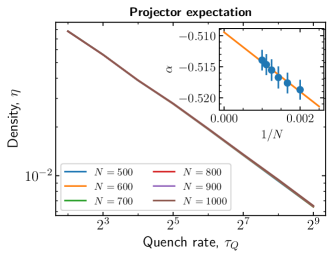
(b)

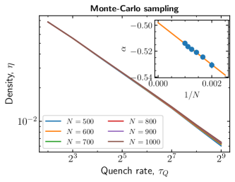
Figure 3: Quench dynamics crossing a QPT involving symmetry protected topological phases as in the SSH model. Numerically obtained defect density scales linearly with the quench rate with the former computed using (a) expectation value of the projector, (b) Monte-Carlo sampling. (Inset) Finite-size scaling analysis to obtain the scaling exponent, $\mu$=(a) 0.509(1) and (b) 0.498(2).

IV.1 Su–Schrieffer–Heeger (SSH) model

The SSH model was introduced in the context of a particle hopping on 1D-lattice Su et al. (1980) and is known to host phases that exhibit SPT order. We consider a time-dependent hardcore bosonic version of the above model, whose Hamiltonian is described by the following,

$$H_{\text{SSH}}(t)=v(t)\sum\limits_{i=1}^{N/2}\sigma_{-}^{2i-1}\sigma_{+}^{2i}+w\sum\limits_{i=1}^{N/2-1}\sigma_{-}^{2i}\sigma_{+}^{2i+1}+\text{h.c.,}$$ (6)

with $v(t)=-t/\tau_{Q}$, $t\in(-\infty,0]$ with $\tau_{Q}$ being the quench rate. The time independent version of Eq. 6 with $v(t)=v$ is exactly solvable in the case of periodic boundary conditions. It hosts gapped phases in the extremal limits of $v\ll w$ and $v\gg w$ with the gap closing at $v=w$. In the case of open boundaries, in the limit of $v\ll w$ it is known that the topological phase is identified by the presence of edge modes, characterized as non-trivial SPT phase. While in the other limit the phase remains topological with no edge modes, characterized as trivial SPT phase with the phase transition occurring at $v=w$ Elben et al. (2020); Jamadagni and Weimer (2022b). For the rest of the analysis we consider the SSH Hamiltonian on a 1D-chain i.e., with open boundaries.

The quench protocol to validate QKZM involves driving an initial state belonging to the trivial SPT phase i.e., the groundstate of Hamiltonian in Eq. 6 at some $v\gg w$. With the final state belonging to the non-trivial SPT phase, we set the reference state as groundstate of the above Hamiltonian at $v=0$, given by the singlet configuration in each of the BA unit cells i.e.,

$$\ket{\phi}_{\text{BA}}=\frac{1}{\sqrt{2}}\prod_{i\in B}\left(\ket{0}_{i}\ket{1}_{i+1}-\ket{1}_{i}\ket{0}_{i+1}\right),$$ (7)

where BA unit cells are as in Fig. 2. Therefore, deviations from the singlet configuration in Eq. 7 give rise to local errors in the corresponding unit cell, that are characterized as density fluctuations, $\ket{\bf{0}}=\ket{00}$, $\ket{\bf{1}}=\ket{11}$ and phase fluctuations, $\ket{\boldsymbol{\plus}}=\frac{1}{\sqrt{2}}(\ket{01}+\ket{10})$.

In the following, we compute the error density and determine the critical exponent by employing techniques as outlined in earlier sections. We assume the state mentioned in Eq. 7 as the reference state and first estimate the local error density by setting $\mathcal{P}_{0}^{i}=\ket{\boldsymbol{\minus}}\bra{\boldsymbol{\minus}}$ in Eq. 3. This further results in the total defect density given by

$$\eta=\frac{1}{N}\sum_{i\in B}\left(1-\braket{\ket{\boldsymbol{\minus}}\bra{\boldsymbol{\minus}}}_{(i,i+1)}\right),$$ (8)

which is due to the fact that each unit cell satisfies the following relation: $\sum\limits_{\lambda}\ket{\lambda}\bra{\lambda}=\mathds{I}$ for $\lambda\in\{\bf{0},\bf{1},\boldsymbol{\plus},\boldsymbol{\minus}\}$. Further, by computing the defect density using the above equation, we estimate the scaling exponent as $\mu=0.509(1)$, see Fig. 3.

Furthermore, it is also possible to determine the critical exponent by employing Monte-Carlo sampling. To this extent, we sample the final evolved state in the excitation basis given by {$\ket{\bf{0}}$, $\ket{\bf{1}}$, $\ket{\boldsymbol{\plus}}$, $\ket{\boldsymbol{\minus}}$} with respect to the earlier defined reference state, see Eq. 7. With the total number of errors given by the sum of density fluctuations, $\{\bf{0},\bf{1}\}$ and phase fluctuations, $\{\boldsymbol{\plus}\}$ results in the critical exponent $\mu=0.498(2)$ shown in Fig. 3. This exemplifies that our method is capable of estimating the expected critical exponent (1/2 for this case) across a topological phase transition Sun et al. (2022).

IV.2 Extended SSH model

In this section, we extend the analysis to the case of the extended SSH model whose Hamiltonian is given by

$$\begin{split}H_{\text{eSSH}}&=\frac{v}{2}\sum\limits_{i=1}^{N/2}\sigma_{x}^{2i-1}\sigma_{x}^{2i}+\sigma_{y}^{2i-1}\sigma_{y}^{2i}+\delta\sigma_{z}^{2i-1}\sigma_{z}^{2i}\\ &+\frac{w}{2}\sum\limits_{i=1}^{N/2-1}\sigma_{x}^{2i}\sigma_{x}^{2i+1}+\sigma_{y}^{2i}\sigma_{y}^{2i+1}+\delta\sigma_{z}^{2i}\sigma_{z}^{2i+1}.\\ \end{split}$$ (9)

We note that setting $\delta=0$ recovers the SSH model discussed in the previous section. The phase diagram of the extended SSH model has been discussed in Refs. Elben et al., 2020; Jamadagni and Weimer, 2022b; Jamadagni et al., 2023 and is known to host trivial and non-trivial SPT phases along with an antiferromagnetic (AFM) phase (as $\delta\rightarrow\infty$), see Fig. 4, for a qualitative sketch of the same. Given the rich phase diagram, we obtain the associated critical exponents by driving across various QPTs. To this extent, we consider two time-dependent variants of the Hamiltonian in Eq. 9 where: (i) $v$ is replaced by a time-dependent function, with $\delta$ and $w$ being a constant, (ii) $v$ and $w$ remain a constant, with $\delta$ being replaced by a time-dependent function. We proceed by presenting a quantitative analysis of the critical behavior using the expectation value of the groundstate projector, while the Monte-Carlo sampling approach has been analyzed in App. A.

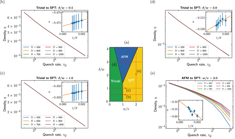
Figure 4: (a) Qualitative groundstate phase diagram of the extended SSH model with arrows indicating the quench dynamics through different QPTs (b, c, d) from trivial to SPT phase by fixing $\delta/w$ to be (b) 0.5, (c) 1.0, (d) 3.0, and (e) from antiferromagnetic (AFM) to SPT phase by fixing $w/v=2$. In the former, the linear scaling of defects (on a $\log-\log$ scale) is in accordance with the QKZM (inset) resulting in the critical exponent, $\mu$ to be (b) 0.4767(1), (c) 0.4328(1), (d)0.521(1). (e) The finite size effects in the AFM-SPT quench are more predominant and are reflected in the deviations from the linear scaling included in the error-estimation of (inset) critical exponent, $\mu$=0.50(2).

IV.2.1 Trivial to SPT transition

We dynamically traverse across the trivial to non-trivial SPT topological transition by employing a quench protocol i.e., by setting $v$ to be $v(t)=-t/\tau_{Q}$, $t\in(-\infty,0]$ and $\delta$ to be a constant belonging to the set $\{0.5,1,3\}$ in Eq. 9. The initial state is chosen as the groundstate of the Hamiltonian in the regime of $v\gg w$ with the final evolved state belonging to the non-trivial SPT phase. The reference state is as introduced in the earlier section via Eq. 7. The above setting leads us to a final evolved state with total defect density given by $\eta$, as in Eq. 8. In Fig. 4, we estimate the critical exponents corresponding to $\delta$ in $\{0.5,1,3\}$. Our numerical experiments show that with interactions turned on, the value of the scaling exponent deviates significantly from 0.5 as in the non-interacting case. We also notice that the value decrease along the transition line $w/v$=1 upto the point where the three phases co-exist and then recovers to 0.5 beyond that.

IV.2.2 AFM to SPT transition

The phase diagram allows for the exploration of critical exponent associated with the AFM-SPT phase transition. To this end, the quench protocol is defined by $\delta(t)=-t/\tau_{Q}$ with $t\in(-\infty,0]$ while fixing $w/v=2$ in Eq. 9. The initial state for evolution is chosen to be the groundstate of $H_{\text{eSSH}}$ in the limits of $\delta\gg w/v$, thereby being smoothly connected to an antiferromagnet. As the system is driven into a non-trivial SPT phase, the reference state remains the same. It might be intuitive to conclude that the total error density is given by Eq. 8. However, on the contrary this is not the case as there are additional corrections involved. It is important to note that the final evolved state encapsulates the errors of the groundstate at finite $w/v$ that need to be subtracted from Eq. 8 to obtain the accurate defect densities. In Fig. 4, we note that by incorporating the additional correction terms we substantiate the predictions as in the QKZM and further obtain the scaling exponent.

IV.3 Cluster state model

One other paradigmatic model that hosts SPT phase is the 1D cluster state model, whose Hamiltonian in the presence of time-dependent perturbation is given by

$$H_{\text{CS}}=-\sum\limits_{i=1}^{N-2}\sigma_{z}^{i}\sigma_{x}^{i+1}\sigma_{z}^{i+2}-g(t)\sum\limits_{j=1}^{N}\sigma_{x}^{j},$$ (10)

where $g(t)$ is as defined in Eq. 1. For the rest of the analysis, we consider the Hamiltonian on a 1D spin chain i.e., with open boundary conditions. In the case of time-independent perturbation, the Hamiltonian hosts a SPT phase at low perturbation strength and a paramagnetic phase at high perturbation strength with a QPT at some perturbation strength Cong et al. (2019). In the absence of perturbation, the groundstate of the Hamiltonian is short-range entangled and protected by a $\mathbb{Z}_{2}\times\mathbb{Z}_{2}$ symmetry Son et al. (2011). The groundstate is also referred to as 1D cluster state with applications in measurement-based quantum computing Nielsen (2006); Deng et al. (2017).

The quench dynamics is performed by choosing the initial state to be the groundstate of the Hamiltonian belonging to the trivial phase. Further, we evolve the above state to a final time wherein the perturbation is completely turned off resulting in a final state belonging to the SPT phase. We further compute the local error density of the final evolved state by setting $\mathcal{P}_{0}^{i}=\frac{\mathds{1}+\sigma_{z}^{i}\sigma_{x}^{i+1}\sigma_{z}^{i+2}}{2}$ in Eq. 3. $\mathcal{P}_{0}^{i}$ projects a given quantum state into the groundstate of the cluster state Hamiltonian, thereby resulting in the total defect density given by

$$\eta=\frac{1}{N}\sum\limits_{i=1}^{N-2}\left(1-\braket{\frac{\mathds{1}+\sigma_{z}^{i}\sigma_{x}^{i+1}\sigma_{z}^{i+2}}{2}}\right).$$

Our numerical analysis shows the critical exponent to be $\mu=0.493(2)$, see Fig. 5. This establishes that the numerical methods introduced here work for wider class of gapped phases that demand multi-site interactions.

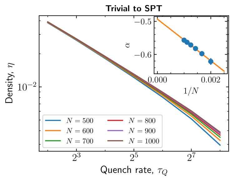
Figure 5: Steering across a trivial-SPT phase transition with the latter characterized by the cluster state Hamiltonian. The predictions of the QKZM remain valid as the logarithm of the defect densities scale linearly with the quench rate in $\log$ scale. We attribute minor deviations from linearity to the finite-size of the system resulting in the (inset) critical exponent, $\mu$=0.493(2).

V Quantifying criticality using digital quantum computers

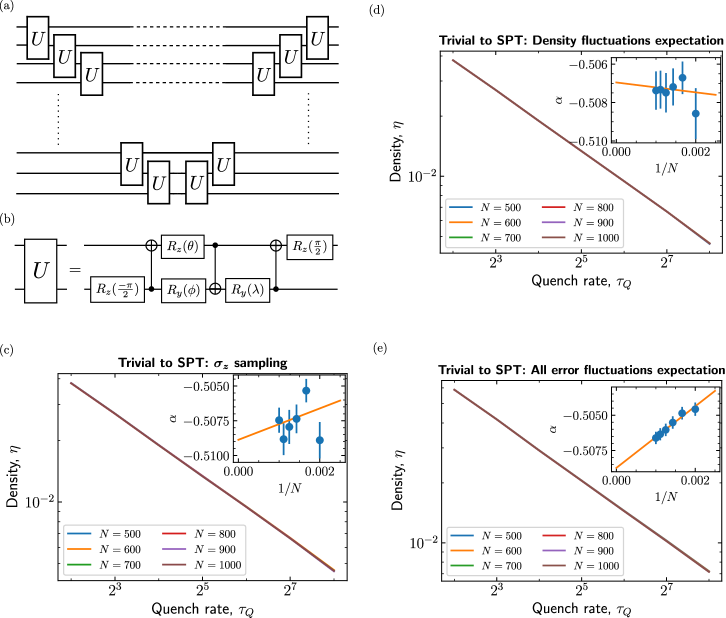
Figure 6: Simulating the quench dynamics involving a topological phase transition as in the extended SSH model on a digital quantum computer. (a) The TEBD protocol comprising of the two-qubit unitary, $U$, see Eq. 12. (b) The decomposition of $U(\alpha,\beta,\gamma)$ in terms of single qubit rotations where $\theta=\frac{\pi}{2}-2\gamma$, $\phi=2\alpha-\frac{\pi}{2}$, $\lambda=\frac{\pi}{2}-2\beta$ and CNOTs. The predicted power law scaling in the QKZM is recovered by considering (c) partial defect density i.e., density fluctuations estimated by sampling in $\sigma_{z}$ basis similar to shot data in experiments, (d) partial defect density by computing the expectation value of the density fluctuations, (e) total defect density determined using the projector expectation value. (Inset) The scaling exponent, $\mu$ obtained by performing finite size scaling resulting in (c) 0.509(3), (d) 0.507(1), (e) 0.508(1) that are in good agreement among themselves while also to the quench protocol employed in Sec. IV.

The recent advancement in quantum hardware has enabled the exploration of several quantum many-body phenomena Smith et al. (2019); de Léséleuc et al. (2019); Semeghini et al. (2021); Satzinger et al. (2021); Iqbal et al. (2023); Li et al. (2023) using Noisy Intermediate Scale Quantum (NISQ) devices Preskill (2018). QKZM has been validated on both analog Keesling et al. (2019) and digital architectures Dupont and Moore (2022). The former provides efficient implementation of quench dynamics while the latter is applicable in a more general setting. For instance, a digital based experiment as well as intensive numerical investigation of the QKZM in TFIM was explored in recent work, see Ref. Dupont and Moore, 2022. Motivated by the above work, we slightly alter our quench protocol that maps two Hamiltonians, $H_{I}$ and $H_{F}$, as follows

$$H(t)=(1-t/\tau_{Q})H_{I}+(1+t/\tau_{Q})H_{F}.$$

We emphasize our method is capable of estimating the critical exponent in models with quantum phases that are beyond the Landau symmetry breaking principle. To exemplify, in this section, we supplement the analysis to the case of the extended SSH Hamiltonian. To this extent, we map the hopping terms in Eq. 9 with strengths $v$ and $w$ to $H_{I}$ and $H_{F}$ respectively resulting in

$$\begin{split}H_{\text{eSSH}}(t,\delta)&=\frac{v^{\prime}(t)}{2}\sum\limits_{i=1}^{N/2}\sigma_{x}^{2i-1}\sigma_{x}^{2i}+\sigma_{y}^{2i-1}\sigma_{y}^{2i}+\delta\sigma_{z}^{2i-1}\sigma_{z}^{2i}\\ &+\frac{w^{\prime}(t)}{2}\sum\limits_{i=1}^{N/2-1}\sigma_{x}^{2i}\sigma_{x}^{2i+1}+\sigma_{y}^{2i}\sigma_{y}^{2i+1}+\delta\sigma_{z}^{2i}\sigma_{z}^{2i+1},\\ \end{split}$$ (11)

with $v^{\prime}(t)=1-t/\tau_{Q}$, $w^{\prime}(t)=1+t/\tau_{Q}$, $t\in[-\tau_{Q},\tau_{Q}]$ and set $\delta=3$ to be a constant, see Fig. 4(a). The initial state that is evolved is identified by the singlet configuration in the AB unit cells i.e., a state belonging to the trivial SPT phase (groundstate of $H_{\text{eSSH}}(-\tau,3)$). The key advantage of using such a protocol is that initial state can be expressed analytically. That is, the groundstate can be expressed as a tensor product of the 2-qubit Bell state ($\frac{1}{\sqrt{2}}(\ket{01}-\ket{10})$) that can be further prepared by using a sequence of single and two qubit gates. With the dynamics driving the above state into a non-trivial SPT phase, the reference state is set to the singlet configuration in the BA unit cells. To simulate the dynamics, as earlier we employ the TEBD protocol, see Fig. 6(a) that involves a two-qubit unitary, $U$, of the form

$$U=\text{exp}[i(\alpha\sigma_{x}\otimes\sigma_{x}+\beta\sigma_{y}\otimes\sigma_{y}+\gamma\sigma_{z}\otimes\sigma_{z})].$$ (12)

The above can be realized on a digital quantum architecture by decomposing it further into single-qubit Pauli rotations and two-qubit Controlled-NOT (CNOT) gates Vatan and Williams (2004); Smith et al. (2019), see Fig. 6(b). We note that the procedure outlined in this section and the simulations thereof, assume an ideal quantum computing architecture. Relaxing the above constraints involves employing additional techniques for instance, fine-tuned finite-size scaling analysis, employing circuit depth reduction techniques to achieve the required evolution in shorter time, and integrating error mitigation strategies, to mention a few. We leave this exploration in the context of topological phases to the future.

In the following, by employing different methods we estimate the defect density. Further, we establish that the scaling exponent determined using partial defect density is in good congruence with that obtained using the total defect density. Importantly among the above methods, the former remains more accessible in an experimental setup.

V.1 Simulating local measurements

In the earlier sections, we have introduced strategies to compute the defect densities based on the expectation value of certain projectors. These projectors in the case of the (extended) SSH model involve two-sites thereby requiring two-qubit measurements that are relatively difficult to realize on digital computing architectures. We relax the above requirement by measuring the final evolved wavefunction belonging to the non-trivial SPT phase in $\sigma_{z}$ basis alone. As noted earlier, this refers to the shot data in a real experiment setting and can be numerically simulated by employing the Monte-Carlo sampling in the $\sigma_{z}$ basis. However, we note that from the above measurement data it is possible to partially capture the error density in terms of the density fluctuations with no access to phase fluctuations due to the single-qubit measurement. Crucially, the partial error density still scales linearly with the quench rate (on the $\log-\log$ scale) further validating the prediction of the QKZM. The critical exponent in the current scenario is given by $\mu=0.509(3)$ as shown in Fig. 6 which is in good agreement with the one obtained earlier in Fig. 4(d). From our numerical experiments, we conclude that single qubit measurements suffice to estimate the critical exponent in the case of topological phase transitions as in the extended SSH model.

V.2 Computing partial and total defect densities

To cross-validate the above results, we compute the expectation value of the final evolved state with respect to different error projectors that are given by $\{\ket{\boldsymbol{0}}\bra{\boldsymbol{0}},\ket{\boldsymbol{1}}\bra{\boldsymbol{1}},\ket{\boldsymbol{\plus}}\bra{\boldsymbol{\plus}}\}$. The total defect density is the sum of the expectation values of the above projectors resulting in Eq. 8. One other quantity that provides an approximation is the partial defect density given by considering only the projectors of density fluctuations similar to the simulated local measurements.

By considering the total defect density, our numerical simulation shows the scaling exponent to be $\mu=0.508(1)$, while scaling analysis of partial defect density results in $\mu=0.507(1)$, see Fig. 6. We highlight the fact that the partial defect density has substantially higher errors as in Fig. 6(c, d) while performing the finite-size scaling analysis in comparison to that of the total defect density as in Fig. 6(e). However, the values of the scaling exponent obtained in three cases agree upto three decimals.

(a)

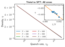
(b)

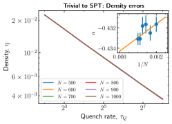
(c)

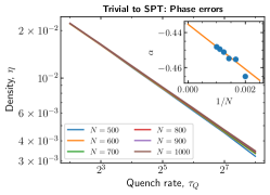
Figure 7: Monte-Carlo sampling to obtain defect densities estimated by considering (a) all errors, (b) density errors, (c) phase errors for the extended SSH model driven into the non-trivial SPT phase. (Inset) Estimating the corresponding critical exponents by performing finite-size analysis leading to $\mu=$ (a) 0.433(1), (b) 0.434(1), (c) 0.435(2) that exhibit agreement with each other and also with the critical exponent obtained based on projector expectation values as in Sec. IV.

VI Summary and Discussion

In summary, we have briefly reviewed the QKZM that establishes a relationship between defect density and quench rates via a critical exponent when a quantum system is driven across a QPT. In the current scenario, in the context of gapped quantum phases, we recast the notion of errors with respect to a given reference state as defects. Further, we computed the defect density based on the expectation value of the projection operators with respect to a predefined reference state. The values from the exact computation provide a means to estimate the critical exponent numerically. In addition, we showed that Monte-Carlo based sampling, akin to measurement in real experiments, provides an alternative to determine the critical exponent.

We adopted the introduced computational strategies to different spin models with QPTs involving local and topological orders. To this extent, we reproduced the scaling critical exponent in the TFIM and SSH models while effectively estimating the same in the extended SSH model and the cluster state model. Towards the end, we proposed a strategy to determine the scaling critical exponent on a digital quantum computer. As an illustration, we have considered the extended SSH model across a QPT involving topological phases.

It is important to note that the methods investigated in this work, can be extended to a wide range of gapped quantum phases. Possible future applications of the computational strategies developed in the current context could include the exploration of (a) QPTs involving intrinsic topological order driven by external fields Jamadagni et al. (2018); Jamadagni and Bhattacharyya (2021), (b) landscape of QKZM in the context of open quantum systems and the phase transitions thereof Jamadagni and Bhattacharyya (2021), and (c) possible relations between QKZM and measurement induced entanglement phase transitions Lavasani et al. (2021a, b). It would also be interesting to quantify criticalities associated with QPTs involving other gapped quantum phases that are easily realizable on upcoming quantum hardware platforms, further allowing us to benchmark their performance.

Appendix A Monte-Carlo sampling of errors in the extended SSH model

We consider the time-dependent extended SSH Hamiltonian, as in Eq. 9 and set $v(t)=-t/\tau_{Q}$, $t\in(-\infty,0]$ i.e., we drive an initial state belonging to the trivial topological phase to a final state in the non-trivial topological phase across the topological phase transition. In Sec. IV.2.1, we determine the criticality by considering the defect density obtained using the strategy based on expectation values of projectors, while in this section, we estimate the criticality by employing the Monte-Carlo method, for the case of $\delta=1$. The main motivation is to benchmark and compare the scaling exponent obtained using only the density errors and only the phase error with that of the full error profile.

As earlier, we drive the system into a non-trivial SPT phase and further sample the final evolved wavefunction in the excitation basis. We compute the total defect density to be the sum of density and phase fluctuations. Further, we determine the critical exponent as shown in Fig. 7. The total defect densities can be approximated by considering either the defect densities or the phase densities. It is crucial to note that predictions of the QKZM still hold in the approximate limit of the total defect densities. In other words, it is possible to estimate the scaling exponent upto good accuracy based on partial defect density as illustrated in Fig. 7.

References

- Kibble (1976) T. W. B. Kibble, Topology of Cosmic Domains and Strings, J. Phys. A 9, 1387 (1976).
- Kibble (1980) T. W. B. Kibble, Some Implications of a Cosmological Phase Transition, Phys. Rept. 67, 183 (1980).
- Zurek (1985) W. H. Zurek, Cosmological Experiments in Superfluid Helium?, Nature 317, 505 (1985).
- Zurek (1993) W. H. Zurek, Cosmic strings in laboratory superfluids and the topological remnants of other phase transitions, Acta Phys. Polon. B 24, 1301 (1993).
- del Campo and Zurek (2014) A. del Campo and W. H. Zurek, Universality of phase transition dynamics: Topological defects from symmetry breaking, International Journal of Modern Physics A 29, 1430018 (2014).
- Ebadi et al. (2021) S. Ebadi et al., Quantum phases of matter on a 256-atom programmable quantum simulator, Nature 595, 227 (2021).
- Zurek et al. (2005) W. H. Zurek, U. Dorner, and P. Zoller, Dynamics of a Quantum Phase Transition, Phys. Rev. Lett. 95, 105701 (2005).
- Dziarmaga (2005a) J. Dziarmaga, Dynamics of a quantum phase transition: exact solution of the quantum Ising model., Physical review letters 95 24, 245701 (2005a).
- Cincio et al. (2007) L. Cincio, J. Dziarmaga, M. M. Rams, and W. H. Zurek, Entropy of entanglement and correlations induced by a quench: Dynamics of a quantum phase transition in the quantum Ising model, Phys. Rev. A 75, 052321 (2007).
- Dziarmaga (2009) J. Dziarmaga, Dynamics of a quantum phase transition and relaxation to a steady state, Advances in Physics 59, 1063 (2009).
- Damski et al. (2011) B. Damski, H. T. Quan, and W. H. Zurek, Critical dynamics of decoherence, Phys. Rev. A 83, 062104 (2011).
- Puebla et al. (2019) R. Puebla, O. Marty, and M. B. Plenio, Quantum Kibble-Zurek physics in long-range transverse-field Ising models, Phys. Rev. A 100, 032115 (2019).
- Kolodrubetz et al. (2012) M. Kolodrubetz, B. K. Clark, and D. A. Huse, Nonequilibrium Dynamic Critical Scaling of the Quantum Ising Chain, Phys. Rev. Lett. 109, 015701 (2012).
- Gong et al. (2015) M. Gong, X. Wen, G. Sun, D.-W. Zhang, D. Lan, Y. Zhou, Y. Fan, Y. Liu, X. Tan, H. Yu, Y. Yu, S.-L. Zhu, S. Han, and P. Wu, Simulating the Kibble-Zurek mechanism of the Ising model with a superconducting qubit system, Scientific Reports 6 (2015).
- Chandran et al. (2012) A. Chandran, A. Erez, S. S. Gubser, and S. L. Sondhi, Kibble-Zurek problem: Universality and the scaling limit, Phys. Rev. B 86, 064304 (2012).
- Rams et al. (2019) M. M. Rams, J. Dziarmaga, and W. H. Zurek, Symmetry Breaking Bias and the Dynamics of a Quantum Phase Transition, Phys. Rev. Lett. 123, 130603 (2019).
- Francuz et al. (2016) A. Francuz, J. Dziarmaga, B. Gardas, and W. H. Zurek, Space and time renormalization in phase transition dynamics, Phys. Rev. B 93, 075134 (2016).
- Schmitt et al. (2021) M. Schmitt, M. M. Rams, J. Dziarmaga, M. Heyl, and W. H. Zurek, Quantum phase transition dynamics in the two-dimensional transverse-field Ising model, Science Advances 8 (2021).
- Dupont and Moore (2022) M. Dupont and J. E. Moore, Quantum criticality using a superconducting quantum processor, Physical Review B 106 (2022).
- Smith et al. (2019) A. Smith, M. S. Kim, F. Pollmann, and J. Knolle, Simulating quantum many-body dynamics on a current digital quantum computer, npj Quantum Information 5 (2019).
- de Léséleuc et al. (2019) S. de Léséleuc, V. Lienhard, P. Scholl, D. Barredo, S. Weber, N. Lang, H. P. Büchler, T. Lahaye, and A. Browaeys, Observation of a symmetry-protected topological phase of interacting bosons with Rydberg atoms, Science 365, 775 (2019).
- Brydges et al. (2019) T. Brydges, A. Elben, P. Jurcevic, B. Vermersch, C. Maier, B. P. Lanyon, P. Zoller, R. Blatt, and C. F. Roos, Probing Rényi entanglement entropy via randomized measurements, Science 364, 260–263 (2019).
- Bhattacharyya et al. (2022) A. Bhattacharyya, L. K. Joshi, and B. Sundar, Quantum information scrambling: from holography to quantum simulators, Eur. Phys. J. C 82, 458 (2022).
- Wei et al. (2023) D. Wei, D. Adler, K. Srakaew, S. Agrawal, P. Weckesser, I. Bloch, and J. Zeiher, Observation of Brane Parity Order in Programmable Optical Lattices, Physical Review X 13, 021042 (2023).
- Keesling et al. (2019) A. Keesling, A. Omran, H. Levine, H. Bernien, H. Pichler, S. Choi, R. Samajdar, S. Schwartz, P. Silvi, S. Sachdev, P. Zoller, M. Endres, M. Greiner, V. Vuletić, and M. D. Lukin, Quantum Kibble–Zurek mechanism and critical dynamics on a programmable Rydberg simulator, Nature 568, 207–211 (2019).
- Dziarmaga (2005b) J. Dziarmaga, Dynamics of a Quantum Phase Transition: Exact Solution of the Quantum Ising Model, Phys. Rev. Lett. 95, 245701 (2005b).
- Polkovnikov (2005) A. Polkovnikov, Universal adiabatic dynamics in the vicinity of a quantum critical point, Phys. Rev. B 72, 161201 (2005).
- Jamadagni and Weimer (2022a) A. Jamadagni and H. Weimer, Operational definition of topological order, Phys. Rev. B 106, 085143 (2022a).
- Jamadagni and Weimer (2022b) A. Jamadagni and H. Weimer, Error-correction properties of an interacting topological insulator, Phys. Rev. B 106, 115133 (2022b).
- Jamadagni et al. (2023) A. Jamadagni, J. Kazemi, and H. Weimer, Learning of error statistics for the detection of quantum phases, Phys. Rev. B 107, 075146 (2023).
- Han et al. (2018) Z.-Y. Han, J. Wang, H. Fan, L. Wang, and P. Zhang, Unsupervised Generative Modeling Using Matrix Product States, Phys. Rev. X 8, 031012 (2018).
- Vidal (2004) G. Vidal, Efficient Simulation of One-Dimensional Quantum Many-Body Systems, Physical Review Letters 93 (2004).
- Fishman et al. (2022) M. Fishman, S. R. White, and E. M. Stoudenmire, The ITensor Software Library for Tensor Network Calculations, SciPost Phys. Codebases , 4 (2022).
- Sachdev (1999) S. Sachdev, Quantum Phase Transitions (Cambridge University Press, 1999).
- Chen et al. (2010) X. Chen, Z.-C. Gu, and X.-G. Wen, Local unitary transformation, long-range quantum entanglement, wave function renormalization, and topological order, Phys. Rev. B 82, 155138 (2010).
- Su et al. (1980) W. Su, J. Schrieffer, and A. Heeger, Soliton excitations in polyacetylene, Phys. Rev. B 22, 2099 (1980).
- Elben et al. (2020) A. Elben, J. Yu, G. Zhu, M. Hafezi, F. Pollmann, P. Zoller, and B. Vermersch, Many-body topological invariants from randomized measurements in synthetic quantum matter, Science Adv. 6, eaaz3666 (2020).
- Sun et al. (2022) Z. Sun, M. Deng, and F. Li, Kibble-Zurek behavior in one-dimensional disordered topological insulators, Phys. Rev. B 106, 134203 (2022).
- Cong et al. (2019) I. Cong, S. Choi, and M. D. Lukin, Quantum convolutional neural networks, Nature Physics 15, 1273–1278 (2019).
- Son et al. (2011) W. Son, L. Amico, and V. Vedral, Topological order in 1D Cluster state protected by symmetry, Quantum Information Processing 11, 1961–1968 (2011).
- Nielsen (2006) M. A. Nielsen, Cluster-state quantum computation, Reports on Mathematical Physics 57, 147–161 (2006).
- Deng et al. (2017) D.-L. Deng, X. Li, and S. Das Sarma, Machine learning topological states, Physical Review B 96 (2017).
- Semeghini et al. (2021) G. Semeghini, H. Levine, A. Keesling, S. Ebadi, T. T. Wang, D. Bluvstein, R. Verresen, H. Pichler, M. Kalinowski, R. Samajdar, A. Omran, S. Sachdev, A. Vishwanath, M. Greiner, V. Vuletić, and M. D. Lukin, Probing topological spin liquids on a programmable quantum simulator, Science 374, 1242 (2021).
- Satzinger et al. (2021) K. J. Satzinger et al., Realizing topologically ordered states on a quantum processor, Science 374, 1237 (2021).
- Iqbal et al. (2023) M. Iqbal, N. Tantivasadakarn, R. Verresen, S. L. Campbell, J. M. Dreiling, C. Figgatt, J. P. Gaebler, J. Johansen, M. Mills, S. A. Moses, J. M. Pino, A. Ransford, M. Rowe, P. Siegfried, R. P. Stutz, M. Foss-Feig, A. Vishwanath, and H. Dreyer, Creation of Non-Abelian Topological Order and Anyons on a Trapped-Ion Processor (2023), arXiv:2305.03766 [quant-ph] .
- Li et al. (2023) A. C. Y. Li, M. S. Alam, T. Iadecola, A. Jahin, J. Job, D. M. Kurkcuoglu, R. Li, P. P. Orth, A. B. Özgüler, G. N. Perdue, and N. M. Tubman, Benchmarking variational quantum eigensolvers for the square-octagon-lattice Kitaev model, Physical Review Research 5 (2023).
- Preskill (2018) J. Preskill, Quantum Computing in the NISQ era and beyond, Quantum 2, 79 (2018).
- Vatan and Williams (2004) F. Vatan and C. Williams, Optimal quantum circuits for general two-qubit gates, Phys. Rev. A 69, 032315 (2004).
- Jamadagni et al. (2018) A. Jamadagni, H. Weimer, and A. Bhattacharyya, Robustness of topological order in the toric code with open boundaries, Phys. Rev. B 98, 235147 (2018).
- Jamadagni and Bhattacharyya (2021) A. Jamadagni and A. Bhattacharyya, Topological phase transitions induced by varying topology and boundaries in the toric code, New Journal of Physics 23, 103001 (2021).
- Lavasani et al. (2021a) A. Lavasani, Y. Alavirad, and M. Barkeshli, Measurement-induced topological entanglement transitions in symmetric random quantum circuits, Nature Physics 17, 342–347 (2021a).
- Lavasani et al. (2021b) A. Lavasani, Y. Alavirad, and M. Barkeshli, Topological Order and Criticality in Monitored Random Quantum Circuits, Phys. Rev. Lett. 127, 235701 (2021b).