Can overfitted deep neural networks in adversarial training generalize? - An approximation viewpoint

Abstract

Adversarial training is a widely used method to improve the robustness of deep neural networks (DNNs) over adversarial perturbations. However, it is empirically observed that adversarial training on over-parameterized networks often suffers from the robust overfitting: it can achieve almost zero adversarial training error while the robust generalization performance is not promising. In this paper, we provide a theoretical understanding of the question of whether overfitted DNNs in adversarial training can generalize from an approximation viewpoint. Specifically, our main results are summarized into three folds: i) For classification, we prove by construction the existence of infinitely many adversarial training classifiers on over-parameterized DNNs that obtain arbitrarily small adversarial training error (overfitting), whereas achieving good robust generalization error under certain conditions concerning the data quality, well separated, and perturbation level. ii) Linear over-parameterization (meaning that the number of parameters is only slightly larger than the sample size) is enough to ensure such existence if the target function is smooth enough. iii) For regression, our results demonstrate that there also exist infinitely many overfitted DNNs with linear over-parameterization in adversarial training that can achieve almost optimal rates of convergence for the standard generalization error. Overall, our analysis points out that robust overfitting can be avoided but the required model capacity will depend on the smoothness of the target function, while a robust generalization gap is inevitable. We hope our analysis will give a better understanding of the mathematical foundations of robustness in DNNs from an approximation view.

Keywords: Deep learning theory, adversarial training, robust overfitting, robust generalization, learning rates

1 Introduction

Deep neural networks (DNNs) have achieved great empirical success but are demonstrated to be susceptible to small perturbations [20]. To be specific, under adversarially chosen, albeit imperceptible, perturbations to their inputs, a.k.a., adversarial examples, a well-performed DNN achieves quite low accuracy on these adversarial examples [42, 21]. This results in a high risk of building robust, secure, trustworthy machine learning systems. To improve the robustness of DNNs, a series of methods are proposed to defend against artificially designed adversarial attacks aiming at fooling the models [22, 8, 33, 51, 15, 1]. Among them, adversarial training [33] is one of the most empirically successful methods to defend against adversarial examples via a min-max optimization.

Mathematically, let $\mathcal{X}\subset\mathbb{R}^{d}$ be the input space, $Y\subset\mathbb{R}$ be the output space, and $\mathcal{F}$ be the hypothesis space, e.g., the class of DNNs. Suppose that the data set $\{(\bm{x}_{i},y_{i})\}_{i=1}^{n}$ are i.i.d. sampled from the true unknown Borel probability distribution $\rho$ on $\mathcal{Z}=\mathcal{X}\times Y$. Then adversarial training aims to solve the following empirical (adversarial) risk minimization under a certain $\ell_{\infty}$ white-box adversarial attack

$$\min_{f\in\mathcal{F}}\frac{1}{n}\sum_{i=1}^{n}\max_{\bm{x}^{\prime}_{i}\in B_{\delta,\infty}(\bm{x}_{i})}\ell\left(f(\bm{x}^{\prime}_{i}),y_{i}\right),$$ (1.1)

where $\ell:\mathbb{R}\times\mathbb{R}\rightarrow\mathbb{R}$ is the loss function which evaluates the cost between the model output and the corresponding label, $B_{\delta,\infty}(\bm{z})=\{\bm{x}:\|\bm{x}-\bm{z}\|_{\infty}\leq\delta\}\cap\mathcal{X}$ is the $\delta$-ball (i.e., the perturbation radius $\delta$) centered at $\bm{z}$ w.r.t. $\ell_{\infty}$ norm.

Taking $\delta=0$ in Equation 1.1, adversarial training degenerates to standard training. Empirical and theoretical studies [50, 3, 6, 43, 53] indicate that DNNs in the over-parameterized regime (i.e., the number of parameters is much larger than the training data size) can achieve zero training error under noisy data, but still generalize well. This is called the benign overfitting phenomenon. When it comes to adversarial training (1.1) with $\delta>0$, empirical observations [41, 35, 36] demonstrate the robust overfitting phenomenon in the over-parameterized regime of adversarial training instead, i.e., overfitting to the training set (achieving small adversarial training error or called train robust error) does harm the robust generalization to a large extent for multiple datasets. Moreover, there exists a large robust generalization gap between the robust generalization and the standard generalization performance [33, 36]. For example, as shown in Figure 1 from [36], the adversarial training can achieve almost zero train robust error, but the test robust error is only nearly 50%, and is much higher than the test standard error (slightly smaller than 20%).

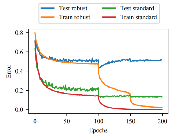
Figure 1: The learning curves of adversarial training on CIFAR-10 with $\delta=8/255$ [36], while CIFAR-10 is 0.212-separated [47].

Recent work [47] finds that real datasets have a natural separation property which is called $\epsilon$-separated: input data points from different classes have at least 2$\epsilon$ distance in the pixel space. For example, on the CIFAR-10 dataset, $\epsilon=0.212$ [47], which is much larger than the commonly used attack level $\delta=8/255$. Due to this well-separated property, ideally, there exist DNNs that can achieve both good robustness and accuracy simultaneously. Nevertheless, this target makes the parameter size of DNNs suffer from the curse of dimensionality as suggested by [29], i.e., an $\exp(\Omega(d))$ lower bound on the network size is inevitable. At first glance, this result is counter-intuitive due to the following two reasons:

• Due to the nice separation property, if the target function is sufficiently smooth or possesses some special structure, the required parameter size of DNNs is not needed in the exponential order of the input dimension $d$ from the perspective of approximation.

• Adversarial training degenerates to the standard training when taking the perturbation radius $\delta=0$, as shown in Equation 1.1. If $\delta$ is sufficiently small, under well-behaved data distribution, robust overfitting can be avoided and benign overfitting can naturally arise without curse of dimensionality, as empirically suggested by [17, 19, 18].

The above two reasons motivate us to carefully rethink the following question:

Can overfitted DNNs in adversarial training generalize with reasonable model complexity?

We give an affirmative answer to this question from an approximation viewpoint by providing a comprehensive analysis to close the gap between theory and practice as much as possible. In our analysis, we consider the data quality, the regularity condition of the target function, and the existence of label noise, and check the existence of the adversarial training global minima with good robust generalization performance. We make the following contributions and findings in this paper:

• We prove by construction that there exist infinitely many over-parameterized DNNs that can achieve zero adversarial training error as well as good robust generalization error of the same order as the lower bound. Such construction is based on the condition on data and perturbation, i.e., the data distribution is of relatively high quality and is well-separated; the perturbation radius of adversarial training is small enough. Furthermore, if the target function is smooth enough, DNNs with $\Omega(n)$ parameters (i.e., linear over-parameterization) are sufficient to achieve both robustness and accuracy simultaneously.

• Our construction of the adversarial training global minima is almost optimal since its robust generalization upper bound matches the order of the lower bound. We also theoretically demonstrate the existence of the robust generalization gap by showing that even for these adversarial training classifiers with good robust performance, their robust generalization error is still worse than their standard generalization error.

Accordingly, our theoretical analysis provides an in-depth understanding of overfitting in adversarial training on over-parameterized DNNs from the perspective of approximation, and provides a relaxed model complexity requirement as well as the best possible robust generalization under this circumstance. Note that our construction is data (distribution)-dependent, which allows us to study the limit performance of DNNs under adversarial training, and hence our analysis points out that robust generalization gap is inevitable. We expect that our results will be beneficial to the dynamics analysis of DNNs under adversarial training algorithms.

The rest of the paper is organized as follows. In Section 2, we give an overview of related works close to our paper. The problem setting and common assumptions for classification and regression is introduced in Section 3. Then in Section 4, we present our main results about robust and standard generalization performance of good adversarial training global minima for the classification tasks. In Section 5, we extend our results in Section 4 to the regression tasks. Section 6 draws a conclusion of this paper. The proofs of our theoretical results can be found in the Appendix.

2 Related Work

It is empirically observed in previous works that adversarial training in over-parameterized regime sometimes might overfit, i.e., the robust overfitting phenomenon [41, 35, 36]. However, the mechanism for this is still unclear. Many works try to figure out the important elements in adversarial training that might lead to robust generalization. [37, 5, 14] manifest that to achieve robust generalization in adversarial training, it requires a larger sample complexity compared with standard training. These results also demonstrate that data distribution is a vital factor in adversarial training. [27] indicates that non-robust features in the data can hurt robust generalization, thus making the data quality significant in adversarial training. [39, 16] also show that robust generalization obtained by adversarial training essentially hinges on the property of the data distribution. [17, 18] further demonstrate that adversarial training can achieve better robust generalization by utilizing data samples with higher quality.

Some works have studied the robust generalization of adversarial training in the under-parameterized regime [28, 49, 46, 34]. For example, [49] presents the adversarial generalization error bounds by adversarial Rademacher complexity, and [46] estimates the bounds of adversarial Rademacher complexity of deep neural networks. However, such adversarial generalization error bounds only work for adversarial training in the under-parameterized regime and are not suitable for the over-parameterized regime. It is still unknown whether benign overfitting exists in adversarial training on over-parameterized DNNs, although there are some attempts in some simple settings. For instance, [10] demonstrates the occurrence of benign overfitting in the adversarially robust linear classification with sub-Gaussian mixture data for both standard and robust generalization. While [30] shows that standard generalization and robust overfitting both happen in adversarial training for the patch data distribution.

Besides, there exist some works close to the scope of this paper that tries to understand the robust generalization from an approximation theory viewpoint [32, 29]. In [32], they study the difference between the robust generalization and standard generalization for the true regression function. In [29], they demonstrate that the network requires $\mathcal{O}(\epsilon^{-d})$ parameters to achieve zero robust generalization for all the $2\epsilon$-separated data distribution when there is no noise. However, the networks they constructed to achieve such robust generalization are irrelevant to the networks learned from adversarial training with the usage of data samples, making their analysis not suitable for the study of the robust generalization for overfitting networks under adversarial training.

3 Problem settings and common assumptions

Here we introduce the common problem settings for classification and regression under adversarial training, e.g., the learning framework, the hypothesis space, and the model formulation. The specific problem settings and assumptions for classification and regression can be found in Section 4.1 and Section 5.1, respectively.

Learning framework: We follow the classical statistical learning framework [13]. Suppose that the data sample $D=\{(\bm{x}_{i},y_{i})\}^{n}_{i=1}\subset\mathcal{Z}^{n}$ are i.i.d. sampled from a Borel probability measure $\rho$ on $\mathcal{Z}=\mathcal{X}\times Y$ with $\mathcal{X}\subset[0,1]^{d}$, $Y=\{-1,1\}$ for binary classification and $Y\subseteq[-M,M]$ with some $M>0$ for regression. For notational simplicity, denoting $X:=\{\bm{x}_{i}\}_{i=1}^{n}$, the separation distance of the input data sample $X$ satisfies [45]

$$q_{X}:=\frac{1}{2}\min_{i\neq j}\|\bm{x}_{i}-\bm{x}_{j}\|_{\infty}\leq n^{-\frac{1}{d}}\,,$$ (3.1)

which is half of the minimal distance between two distinct input data samples admitting an upper bound w.r.t. $n$ and $d$.

Denote $\rho(y|\bm{x})$ as the conditional distribution at $\bm{x}\in\mathcal{X}$ induced by $\rho$, $\rho_{X}$ as the marginal distribution of $\rho$ on $\mathcal{X}$, and $(L^{2}_{\rho_{X}},\parallel\cdot\parallel_{\rho})$ as the Hilbert space of square-integrable functions with respect to $\rho_{X}$. The objective of learning for classification or regression is to find a learning model that is a good approximation of the “target function”, which is defined as the conditional mean $f_{\rho}(\bm{x})=\int_{Y}yd\rho(y|\bm{x})$. Here the used learning model is a fully-connected deep neural network as described below.

Model formulation of DNNs: Regarding the learning model, we consider standard fully-connected deep neural networks (FNNs) with the ReLU activation function in this paper. Denote the affine operator $\mathcal{A}_{\ell}:\mathbb{R}^{d_{\ell-1}}\to\mathbb{R}^{d_{\ell}}$ as $\mathcal{A}_{\ell}(\bm{x})=\bm{W}_{\ell}\bm{x}+\bm{b}_{\ell}$, where $\bm{W}_{\ell}\in\mathbb{R}^{d_{\ell}\times d_{\ell-1}}$ is the weight matrix and $\bm{b}_{\ell}\in\mathbb{R}^{d_{\ell}}$ is the bias vector. A deep ReLU FNN with depth $L$ and width $\{d_{\ell}\}_{\ell=1}^{L}$ is defined as

$$f(\bm{x})=c\cdot\sigma\circ\mathcal{A}_{L}\circ\sigma\circ\mathcal{A}_{L-1}\circ\cdots\circ\sigma\circ\mathcal{A}_{1}(\bm{x})\,,$$ (3.2)

where $d_{0}=d$, $\bm{c}\in\mathbb{R}^{d_{L}}$ is the coefficient vector, $\{\bm{W}_{\ell}\}_{\ell=1}^{L}$ are the weight matrices and $\{\bm{b}_{\ell}\}_{\ell=1}^{L}$ are the bias vectors. The number of parameters in this network is

$$\mathcal{N}=d_{L}+\sum_{\ell=1}^{L}(d_{\ell-1}d_{\ell}+d_{\ell})\,.$$ (3.3)

We denote the hypothesis space $\mathcal{F}_{\vec{d},L}$ as the collection of all deep ReLU FNNs with the form (3.2).

Common assumptions: In the next, we make two assumptions: one is about the distortion of $L_{\rho_{X}}$ with respect to the Lebesgue measure [12] and the other one is the regularity assumption of the “target function”.

Assumption 1.

[40, 12, non-irregularity of $\rho_{X}$] Let $J_{\rho}$ be the identity mapping $J_{\rho}:L^{1}(\mathcal{X})\to L_{\rho_{X}}^{1}(\mathcal{X})$ and $\|J_{\rho}\|$ be the operator norm. Similarly, we denote $\bar{J}_{\rho}$ as the identity mapping $\bar{J}_{\rho}:L_{\rho_{X}}^{1}(\mathcal{X})\to L^{1}(\mathcal{X})$, and $\|\bar{J}_{\rho}\|$ as the corresponding operator norm. We assume that

$$\|J_{\rho}\|<\infty,\quad\|\bar{J}_{\rho}\|<\infty.$$ (3.4)

Moreover, we denote $\Phi_{\rho}$ as the set of $\rho_{X}$ that satisfies 1.

Remark 1.

This assumption on the marginal distribution $\rho_{X}$ is similar as [40, 12] to ensure that $\rho_{X}$ is not that irregular. Admittedly, it is a little stronger than the standard assumption that $\rho_{X}$ is absolutely continuous with respect to the Lebesgue measure. However, this assumption can be satisfied when $\rho_{X}$ is some common distribution with bounded support, e.g., uniform distribution.

Hölder continuity: We assume the “target function” satisfies some smoothness level which is of interest for ease of analysis. We describe it in Hölder spaces, i.e., the $\alpha$-Hölder continuous functions $W_{\infty}^{\alpha}(\mathcal{X})$ with $\alpha>0$ [48, 38]. To be specific, for $\alpha\in(0,1]$, $W_{\infty}^{\alpha}(\mathcal{X})$ consists of $\alpha$-Lipschitz functions with the norm

$$\lVert f\rVert_{W_{\infty}^{\alpha}}=\lVert f\rVert_{\infty}+\lvert f\rvert_{W_{\infty}^{\alpha}}\quad\mbox{with}~{}\lVert f\rVert_{\infty}=\sup_{\bm{x}\in\mathcal{X}}\lvert f(\bm{x})\rvert,\quad\lvert f\rvert_{W_{\infty}^{\alpha}}=\sup_{\bm{x}\neq\bm{y}}\frac{\left|f(\bm{x})-f(\bm{y})\right|}{\left\|\bm{x}-\bm{y}\right\|_{2}^{\alpha}}\,.$$

Note that $\lvert f\rvert_{W_{\infty}^{\alpha}}$ is the semi-norm. For $\alpha=s+t$ with $s\in\mathbb{N}$ and $t\in(0,1]$, $W_{\infty}^{\alpha}(\mathcal{X})$ consists of $s$-times differentiable functions whose partial derivatives of order $s$ are $t$-Lipschitz functions, with an equivalent norm $\lVert f\rVert_{W_{\infty}^{\alpha}}=\sum_{\|\bm{k}\|_{2}<s}\lVert D^{\bm{k}}f\rVert_{\infty}+\sum_{\|\bm{k}\|_{2}=s}\lVert D^{\bm{k}}f\rVert_{W_{\infty}^{t}}$. For certain regularity assumptions for the “target function”, we will detail them in the respective sections.

4 Main Results for Classification

In this section, we demonstrate the main results of adversarial training for classification: there exist infinitely many classifiers obtained by adversarial training with commonly used loss functions, such as hinge loss and logistic loss, that can achieve arbitrarily small adversarial training error and good robust generalization error with the same order of the lower bound when the data distribution is well-separated and of relatively high quality.

4.1 Problem settings and notations

For binary classification, the objective of learning is to find the best classifier (Bayes rule) $f_{c}$ on $\mathcal{X}$ defined by

$$f_{c}(\bm{x})=\begin{cases}1,&\hbox{if}\ \rho(y=1|\bm{x})\geq\rho(y=-1|\bm{x})\,,\\ -1,&\hbox{if}\ \rho(y=1|\bm{x})<\rho(y=-1|\bm{x})\,,\end{cases}$$ (4.1)

which is the minimizer of the standard misclassification error with the 0-1 loss

$$\mathcal{R}(f):=\int_{\mathcal{Z}}\mathbbm{1}_{\{yf(x)=-1\}}d\rho\,.$$ (4.2)

Based on the observed data sample, a learning algorithm aims at finding a function $f$ in a hypothesis space $\mathcal{F}$ such that the classifier $\text{sgn}(f)$ is a good approximation of the Bayes rule $f_{c}$. In the next, we introduce the empirical/expected risk for analysis.

Empirical and expected risks for standard and robust learning: Since the 0-1 loss is non-convex and discontinuous, it is difficult to optimize. Instead, one can utilize some surrogate loss functions $\phi$ to learn an estimator from the data sample $D$, such as hinge loss, least squares loss, and logistic loss. To be specific, we define the $\phi$-risk and its minimum $f_{\rho}^{\phi}$ as

$$\quad f_{\rho}^{\phi}:=\operatorname*{arg\,min}_{f}\mathcal{E}^{\phi}(f)\,,\quad\mbox{with}~{}\mathcal{E}^{\phi}(f):=\int_{\mathcal{Z}}\phi\left(yf(\bm{x})\right)\mathrm{d}\rho\,.$$ (4.3)

Actually, $f_{\rho}^{\phi}$ has the closed form for many commonly used surrogate loss functions [52]. For example, denoting $\eta(\bm{x}):=\rho(y=1|\bm{x})$, we have $f_{\rho}^{\phi}=2\eta-1=f_{\rho}$ for the least squares loss; we have $f_{\rho}^{\phi}=\text{sgn}(2\eta-1)=f_{c}$ for the hinge loss. The standard empirical risk minimization (ERM) algorithm aims to minimize the empirical $\phi$-risk over the hypothesis space being the deep ReLU FNNs $\mathcal{F}_{\vec{d},L}$

$$\widehat{f}_{D,\phi}=\operatorname*{arg\,min}_{f\in\mathcal{F}_{\vec{d},L}}\widehat{\mathcal{E}}_{D}^{\phi}(f),\quad\mbox{with}~{}\widehat{\mathcal{E}}_{D}^{\phi}(f):=\frac{1}{n}\sum_{i=1}^{n}\phi\left(y_{i}f(\bm{x}_{i})\right)\,.$$ (4.4)

We desire that the classifier $\text{sgn}(\widehat{f}_{D,\phi})$ can approach the Bayes rule when the number of samples is large enough, in the sense that the standard excess misclassification error $\mathcal{R}(\text{sgn}(\widehat{f}_{D,\phi}))-\mathcal{R}(f_{c})$ is small.

The above definitions can be extended to the adversarial training setting where we apply the robust loss instead of the standard loss. In this paper, we consider the $\ell_{\infty}$ white-box adversarial attack, where the adversary can use small perturbations of the inputs within some $\ell_{\infty}$ ball to maximize the standard loss. In order to defend against such adversarial attack, our goal is to minimize the adversarial misclassification error (robust generalization)

$$\mathcal{R}^{\delta}(f):=\int_{\mathcal{Z}}\max_{\bm{x}^{\prime}\in B_{\delta,\infty}(\bm{x})}\mathbbm{1}_{\{yf(\bm{x}^{\prime})=-1\}}d\rho\,,$$ (4.5)

which measures the robust generalization performance, and we denote the best robust classifier as $f_{c}^{\delta}=\operatorname*{arg\,min}_{f}\mathcal{R}^{\delta}(f)$. Similarly, the adversarial training implements the ERM algorithm by minimizing the empirical adversarial $\phi$-risk

$$\widehat{\mathcal{E}_{D}^{\phi,\delta}}(f):=\frac{1}{n}\sum_{i=1}^{n}\max_{\bm{x}^{\prime}_{i}\in B_{\delta,\infty}(\bm{x}_{i})}\phi\left(y_{i}f(\bm{x}^{\prime}_{i})\right)\,,$$ (4.6)

over the hypothesis space $\mathcal{F}_{\vec{d},L}$. Moreover, we denote $\widetilde{\Delta}_{\delta,\vec{d},L}$ as the set of the global minima of the optimization problem Equation 4.6 for adversarial training, i.e.,

$$\widetilde{\Delta}_{\delta,\vec{d},L}:=\left\{\widehat{f}_{D}^{\delta}:\widehat{f}_{D}^{\delta}=\operatorname*{arg\,min}_{f\in\mathcal{F}_{\vec{d},L}}\widehat{\mathcal{E}_{D}^{\phi,\delta}}(f)\right\}\,.$$ (4.7)

4.2 Assumptions

In this subsection, apart from assumptions discussed in Section 3, we additionally require some assumptions with regard to the data separation and quality. All of them are related to how to set the Borel measure $\rho$ to control the data generation process.

First, we make the following assumption related to well-separated data in $\mathcal{X}$.

Assumption 2 (well separated data).

Denote $A=\{\bm{x}\in\mathcal{X}:f_{c}(\bm{x})=1\}$ and $B=\{\bm{x}\in\mathcal{X}:f_{c}(\bm{x})=-1\}$, clearly we have $\mathcal{X}=A\cup B$. The two classes are $2\delta$-separated if

$$\|\bm{x}_{A}-\bm{x}_{B}\|_{\infty}\geq 2\delta,\quad\forall\bm{x}_{A}\in A,\ \bm{x}_{B}\in B\,.$$ (4.8)

Remark 2.

This assumption is needed to guarantee the existence of a robust classifier, which is also considered in previous theoretical work [29]. This assumption has been discussed in the introduction and is demonstrated to be attainable. For real data sets, different classes tend to be well-separated, and the perturbation radius is typically much smaller than the separation distance of different classes [47]. For example, on CIFAR-10, the minimum separation distance is 0.21, which is much larger than the perturbation radius $\delta=8/255$.

However, merely with 2, [29] show that a worst-case requirement on the model complexity suffers from the curse of dimensionality. This is because no regularity assumption is added to the target function. To obtain a relaxed model complexity requirement, apart from the $\alpha$-Hölder continuous assumption as mentioned in Section 3, we additionally require that the Bayes rule is confident in its prediction.

Assumption 3 (regularity assumption and high confidence of the Bayes rule).

We assume that $\eta\in W^{\alpha}_{\infty}(\mathcal{X})$ with $\alpha\in\mathbb{N}$. Besides, there exists some arbitrary small constant $\zeta>0$ such that

$$\left|\eta(\bm{x})-0.5\right|>\zeta,\quad\forall\bm{x}\in\mathcal{X}\,.$$ (4.9)

Remark 3.

This assumption is also reasonable since it assures that for the true data distribution $\rho$, if the Bayes rule $f_{c}$ indicates that the label of the input $\bm{x}$ belongs to one class, then the probability that it belongs to this class should not be that close to $0.5$. That means the true classifier should have some confidence in its classification for every input data. In other words, this assumption ensures that the data distribution is of relatively high quality. Similar notations to measure the quality of data samples and features are utilized in [27, 18].

4.3 Generalization analysis of adversarial training global minima on over-parameterized FNNs

In this subsection, we indicate that overfitted DNNs in adversarial training can generalize under the circumstances that the data distribution is of relatively high quality and is well-separated, the perturbation radius is small enough, and the number of free parameters in DNNs is large enough. To begin with, we utilize the following error decomposition method for the excess adversarial misclassification error.

Proposition 1.

Let $f_{c}^{\delta}:=\operatorname*{arg\,min}_{f}\mathcal{R}^{\delta}(f)$. For any classifier $f$, we have

$$\mathcal{R}^{\delta}(f)-\mathcal{R}^{\delta}(f_{c}^{\delta})\leq\mathcal{R}^{\delta}(f)-\mathcal{R}(f)+\mathcal{R}(f)-\mathcal{R}(f_{c})\,.$$ (4.10)

Moreover, we always have $\mathcal{R}(f)\leq\mathcal{R}^{\delta}(f)$.

Proof of Proposition 1.

We use the following error decomposition and the fact that $\mathcal{R}(f_{c})\leq\mathcal{R}(f_{c}^{\delta})$ to get

$$\mathcal{R}^{\delta}(f)-\mathcal{R}^{\delta}(f_{c}^{\delta}) =\mathcal{R}^{\delta}(f)-\mathcal{R}(f)+\mathcal{R}(f)-\mathcal{R}(f_{c})$$

$$+\mathcal{R}(f_{c})-\mathcal{R}(f_{c}^{\delta})+\mathcal{R}(f_{c}^{\delta})-\mathcal{R}^{\delta}(f_{c}^{\delta})$$

$$\leq\mathcal{R}^{\delta}(f)-\mathcal{R}(f)+\mathcal{R}(f)-\mathcal{R}(f_{c})+\mathcal{R}(f_{c}^{\delta})-\mathcal{R}^{\delta}(f_{c}^{\delta})\,.$$

Moreover, for any $\bm{x}\in\mathcal{X},y\in\{-1,1\}$, $\phi(yf(\bm{x}))\leq\max_{\bm{x}^{\prime}\in B_{\delta,\infty}(\bm{x})}\phi(yf(\bm{x}^{\prime}))$ holds for any $f$, then we get $\mathcal{R}(f)\leq\mathcal{R}^{\delta}(f)$. Therefore, we also have $\mathcal{R}(f_{c}^{\delta})\leq\mathcal{R}^{\delta}(f_{c}^{\delta})$. Thus we complete the proof. ∎

Remark 4.

Since $\mathcal{R}(f)\leq\mathcal{R}^{\delta}(f)$ for any $f$, the robust generalization of any function is always larger than its standard generalization. This lower bound of robust generalization error together with the upper bound of it in Proposition 1 partially illustrates the robust generalization gap phenomenon. Moreover, Proposition 1 shows that the robust generalization of a classifier $f$ is bounded by the sum of its standard generalization $\mathcal{R}(f)-\mathcal{R}(f_{c})$ and its robustness $\mathcal{R}^{\delta}(f)-\mathcal{R}(f)$. Roughly speaking, the existence of such an additional robustness term of the classifier might result in lower robust generalization performance compared with the standard generalization performance in adversarial training. We explicitly demonstrate the existence of the robust generalization gap hereinafter.

Based on the above error decomposition, we are now ready to bound the adversarial misclassification error of good adversarial training classifiers on over-parameterized deep ReLU FNNs. The following theorem is one main result of our paper with the surrogate loss being the hinge loss.

Theorem 1 (upper bound under the hinge loss).

Let the surrogate loss function $\phi(t)=\max\{1-t,0\}$ be the hinge loss. Suppose that the Borel measure $\rho$ satisfies 1, 2, 3 with $\eta\in W^{\alpha}_{\infty}(\mathcal{X})$ and $\alpha\in\mathbb{N}$, taking the perturbation radius $\delta<\frac{q_{X}}{3}\leq\frac{1}{3}n^{-\frac{1}{d}}$, then for any $C_{0}\in(0,1]$, there exist infinity many adversarial training global minima $\widehat{f}_{D}^{over}\in\tilde{\Delta}_{\delta,\vec{d},L}$ with depth $L=\mathcal{O}\left(\log\frac{1}{\zeta}\right)$, width $d_{1}=\mathcal{O}\left(\zeta^{-\frac{d}{\alpha}}\log\frac{1}{\zeta}+n\right)$, $d_{2},\dots,d_{L}=\mathcal{O}\left(\zeta^{-\frac{d}{\alpha}}\log\frac{1}{\zeta}\right)$, and non-zero free parameters $\mathcal{O}\left(\zeta^{-\frac{d}{\alpha}}\log\frac{1}{\zeta}+n\right)$, such that

$$\mathbb{E}\left[\mathcal{R}\left(\text{sgn}\left(\widehat{f}_{D}^{over}\right)\right)-\mathcal{R}(f_{c})\right]\leq 2\|J_{\rho}\|\left((2+2C_{0})\delta\right)^{d}n\,,$$ (4.11)

and

$$\mathbb{E}\left[\mathcal{R}^{\delta}\left(\text{sgn}\left(\widehat{f}_{D}^{over}\right)\right)-\mathcal{R}^{\delta}(f_{c}^{\delta})\right]\leq 3\|J_{\rho}\|\left((4+2C_{0})\delta\right)^{d}n\,.$$ (4.12)

Remark 5.

We make the following remarks on the derived results:
1) This theorem shows that for the $2\delta$-separated data distribution with relatively high quality (with the quality measured by $\zeta$), when the perturbation radius $\delta$ is small enough, and the complexity of the neural network is large enough depending on the data distribution’s quality and regularity, there exist infinitely many adversarial training global minima with clean and robust generalization performance.
2) This result partially indicates the importance of the data distribution’s quality in adversarial training, which is consistent with the empirical findings that adversarial training with high-quality data has better robust performance compared with using low-quality data, and it can largely alleviate the robust overfitting problem [17].
3) Moreover, when the data distribution’s quality is higher ($\zeta$ is larger) or its regularity is larger ($\alpha$ is larger), the requirement of the model complexity is smaller, to ensure the existence of adversarial training global minima with good robust generalization performance. Such requirement of model complexity is better than $\mathcal{O}(\delta^{-d})$ stated in [29] when the regularity is large. They only consider the worst case of model complexity to obtain good robust generalization for all $2\delta$-separated data, without consideration of the regularity of the target function.

Remark 6.

We make the following remarks on the derived bounds w.r.t. the perturbation radius:
1) The perturbation radius plays a significant role in the adversarial training. The well-separated training set is a standard assumption in the over-parameterized literature. Here we require that the perturbation radius is smaller than a third of the training set’s separation distance. Such assumption can be satisfied when the input dimension $d$ is large, e.g., for CIFAR-10 dataset $d=3072$, then $n^{-\frac{1}{d}}$ can be nearly 1, while $\delta$ is typically at most 0.05 in practice [24]. It is also exhibited in [39] that for the same MNIST task, adversarial training on the MNIST dataset with higher resolution can achieve higher adversarial robustness.
2) Our robust generalization error upper bound suggests that the robust generalization error of adversarial training can be smaller when the perturbation radius is relatively smaller. This is partially derived from the expansion of the memorization of the label noise at one point to the $\delta$ ball while overfitting occurs in adversarial training. Empirical results also suggest that such label noise would be larger with usage of larger perturbation radius in adversarial training, thus resulting in larger variance and the robust overfitting phenomenon [19, 18].

Next, we also provide a lower bound of the adversarial misclassification error for all the adversarial training global minima on over-parameterized deep ReLU nets with the hinge loss.

Theorem 2 (lower bound under the hinge loss).

Under the same setting of Theorem 1, then for any adversarial training global minimum $\widehat{f}_{D}^{over}\in\tilde{\Delta}_{\delta,\vec{d},L}$ with non-zero free parameters $\mathcal{O}\left(\zeta^{-\frac{d}{\alpha}}\log\frac{1}{\zeta}+n\right)$, we have

$$\mathbb{E}\left[\mathcal{R}^{\delta}\left(\text{sgn}\left(\widehat{f}_{D}^{over}\right)\right)-\mathcal{R}^{\delta}(f_{c}^{\delta})\right]\geq 2\zeta\|\bar{J}_{\rho}\|\mathcal{R}(f_{c})(4\delta)^{d}n\,.$$ (4.13)

Remark 7.

Comparing Equation 4.11 with Equation 4.13, since $C_{0}\in(0,1]$ can be arbitrarily small, we have that the excess standard misclassification error of good adversarial training global minima can be smaller than $\mathcal{O}((2\delta)^{d}n)$, while their excess adversarial misclassification error are larger than $\mathcal{O}((4\delta)^{d}n)$. Such difference is because, for the adversarial training global minima, their standard generalization performance would only be influenced by the memorization of noise in the $\delta$-ball around the input training data points, while their robust generalization performance would be influenced by the $2\delta$-ball around the input training data points. This explicitly demonstrates the existence of the robust generalization gap.

Since $\mathcal{R}(f_{c})$ is the misclassification error of the Bayes rule which also measures the quality of the data distribution, this lower bound again demonstrates the importance of the perturbation radius and the data distribution’s quality on the adversarial training as is exhibited in [17, 19, 18]. Furthermore, comparing Equation 4.12 with Equation 4.13, since $C_{0}\in(0,1]$ can be arbitrarily small, the excess adversarial misclassification error upper bounds of adversarial training global minima we derived above matches the order of the lower bound, showing that our construction is almost optimal.

Moreover, the above adversarial misclassification error bound results under the hinge loss can be extended to the other commonly used loss functions for the classification tasks, e.g., the logistic loss. We can also demonstrate that there still exist infinitely many adversarial training global minima that can achieve arbitrarily small adversarial training error and good robust generalization error. The details are specified in Section A.3.

5 Main Results on Regression Tasks

In this section, we extend our results in Section 4 to the regression tasks. Specifically, under the over-parameterized regime, we first demonstrate the existence of infinitely many adversarial training global minima that can achieve near-optimal rates of convergence for the standard generalization, when the perturbation radius is small enough. Then, we also show that there are infinitely many adversarial training global minima that can obtain good robust generalization errors of the same order as the lower bound when the perturbation radius satisfies some conditions.

5.1 Notations and assumptions

For regression under the least squares loss, the objective of learning is to find the target function $f_{\rho}$, which minimizes the standard generalization error

$$\mathcal{E}(f):=\int_{\mathcal{Z}}(f(\bm{x})-y)^{2}d\rho\,.$$ (5.1)

We can write it in the style of the data generation process, i.e., $y=f_{\rho}(\bm{x})+\epsilon$ for any data point $(\bm{x},y)\sim\rho$, where the noise $\epsilon$ is assumed to have zero mean with $\mathbb{E}[\epsilon]=0$ and bounded variance with $\mathbb{V}[\epsilon]=\sigma^{2}$.

The ERM algorithm under the least squares loss aims to minimize the empirical generalization error

$$\widehat{\mathcal{E}}_{D}(f):=\frac{1}{n}\sum_{i=1}^{n}(f(\bm{x}_{i})-y_{i})^{2},$$ (5.2)

over the hypothesis space $\mathcal{F}_{\vec{d},L}$.

The above definitions can also be extended to the adversarial training setting in the regression task as what is done in Section 4 for the classification task. To defend against the $\ell_{\infty}$ white-box adversarial attack, our goal is to minimize the adversarial generalization error $\mathcal{E}^{\delta}(f)$ with

$$f_{\rho}^{\delta}(\bm{x}):=\operatorname*{arg\,min}_{f}\mathcal{E}^{\delta}(f)\quad\mbox{with}~{}\mathcal{E}^{\delta}(f):=\int_{\mathcal{Z}}\max_{\bm{x}^{\prime}\in B_{\delta,\infty}(\bm{x})}\left(f(\bm{x}^{\prime})-y\right)^{2}d\rho\,,$$ (5.3)

where $f_{\rho}^{\delta}(\bm{x})$ is denoted as the robust target function. Correspondingly, the adversarial training implements the ERM algorithm that minimizes the empirical adversarial generalization error

$$\widehat{\mathcal{E}_{D}^{\delta}}(f):=\frac{1}{n}\sum_{i=1}^{n}\max_{\bm{x}^{\prime}_{i}\in B_{\delta,\infty}(\bm{x}_{i})}\left(f(\bm{x}^{\prime}_{i})-y_{i}\right)^{2},$$ (5.4)

over the hypothesis space $\mathcal{F}_{\vec{d},L}$. Moreover, we denote $\Delta_{\delta,\vec{d},L}$ as the set of the global minima of the optimization problem Equation 5.4 for adversarial training, i.e.,

$$\Delta_{\delta,\vec{d},L}:=\left\{\widehat{f}_{D}^{\delta}:\widehat{f}_{D}^{\delta}=\operatorname*{arg\,min}_{f\in\mathcal{F}_{\vec{d},L}}\widehat{\mathcal{E}_{D}^{\delta}}(f)\right\}.$$ (5.5)

For regression, the required assumptions are weaker than that of classification in Section 4.1. The reason is that in the regression task, we measure the squares loss within the $\delta$-ball, which can remain small if $f$ is smooth. Whereas in the classification task, even if $f$ changes a little in the $\delta$-ball, its sign can vary from $-1$ to $+1$ if its value is close to 0. Here we only need the distortion assumption in 1 and the the regularity assumption for $f_{\rho}$ stated in Section 3.

5.2 Standard generalization analysis of adversarial training estimators on over-parameterized FNNs

In this subsection, we study the standard generalization error analysis of the estimators obtained by adversarial training on over-parameterized deep ReLU FNNs, and answer the question of whether they can achieve good learning rates as the standard ERM estimators on under-parameterized deep ReLU FNNs do.

Suppose that the target function $f_{\rho}\in W_{\infty}^{\alpha}(\mathcal{X})$ with $\alpha>0$. Denote $\Psi_{D}$ as the set of regression function estimators that are derived according to the data sample $D$ with size $n$. The classical statistical results [25] demonstrated that the optimal rates of convergence that can be achieved by a learning algorithm is

$$\inf_{f_{D}\in\Psi_{D}}\sup_{f_{\rho}\in W_{\infty}^{\alpha}(\mathcal{X}),\rho_{X}\in\Phi_{\rho}}\mathbb{E}\left[\mathcal{E}(f_{D})-\mathcal{E}(f_{\rho})\right]=\Theta\left(n^{-\frac{2\alpha}{2\alpha+d}}\right).$$ (5.6)

With a truncated operator introduced for the estimator

$$\pi_{M}f(\bm{x}):=\left\{\begin{array}[]{ll}f(\bm{x}),&\hbox{if}\ |f(\bm{x})|\leq M,\\ M,&\hbox{if}\ f(\bm{x})>M,\\ -M,&\hbox{if}\ f(\bm{x})<-M\,,\end{array}\right.$$

recent works indicate that all the truncated estimators (with the truncated operator applied on the estimators) obtained by the standard ERM algorithm on under-parameterized deep ReLU FNNs can achieve near-optimal learning rates [38, 26].

Lemma 1 ([38, 26]).

Suppose that the target function $f_{\rho}\in W_{\infty}^{\alpha}(\mathcal{X})$ with $\alpha>0$, there exists some under-parameterized FNN structure $\mathcal{F}_{\vec{d},L}$ with $L\sim\log n$, $d_{1}=\mathcal{O}(n^{\frac{d}{2\alpha+d}})$ , and $d_{2},d_{3},\dots d_{L}=\mathcal{O}\left(\log n\right)$, such that for $f_{D}^{under}=\pi_{M}\operatorname*{arg\,min}_{f\in\mathcal{F}_{\vec{d},L}}\widehat{\mathcal{E}}_{D}(f)$, i.e., any truncated estimators of the standard ERM algorithm, we have

$$\sup_{f_{\rho}\in W_{\infty}^{\alpha}(\mathcal{X}),\rho_{X}\in\Phi_{\rho}}\mathbb{E}\left[\mathcal{E}\left(f_{D}^{under}\right)-\mathcal{E}\left(f_{\rho}\right)\right]\leq C_{1}\left(\frac{n}{\log n}\right)^{-\frac{2\alpha}{2\alpha+d}},$$ (5.7)

where $C_{1}$ is a constant independent of $n$.

However, the generalization performance of the global minima of standard ERM algorithms on over-parameterized deep ReLU FNNs is still theoretically unclear. The empirical results exhibit that some ERM global minima on over-parameterized deep ReLU FNNs can not only interpolate the training data but also achieve good generalization performance [4, 50], the occurrence of such benign overfitting phenomenons are further theoretically studied by many other works [3, 7, 31].

In this section, we try to further understand the standard generalization performance of adversarial training on over-parameterized FNNs, extending previous work [31] from the standard ERM algorithm to the adversarial training. Our result indicates that under the over-parameterized regime, there do exist infinitely many adversarial training estimators that can achieve zero adversarial training error as well as the near-optimal rates of convergence for the standard generalization error, i.e., clean accuracy is promising, when the perturbation radius is small enough.

Theorem 3.

Suppose that the target function $f_{\rho}\in W_{\infty}^{\alpha}(\mathcal{X})$ with $\alpha>0$, and the marginal distribution $\rho_{X}$ satisfies 1. If perturbation radius $\delta<\min\left\{\frac{q_{X}}{3},n^{-\frac{2\alpha}{(2\alpha+d)d}-\frac{1}{d}}\right\}$, then there exist infinity many adversarial training estimators $\widehat{f}_{D}^{over}\in\Delta_{\delta,\vec{d},L}$ with depth $L=\mathcal{O}\left(\log n\right)$, and width $d_{1}=\mathcal{O}\left(n\right)$, $d_{2},\dots,d_{L}=\mathcal{O}\left(\log n\right)$, such that

$$\sup_{f_{\rho}\in W_{\infty}^{\alpha}(\mathcal{X}),\rho_{X}\in\Phi_{\rho}}\mathbb{E}\left[\mathcal{E}\left(\widehat{f}_{D}^{over}\right)-\mathcal{E}\left(f_{\rho}\right)\right]\leq C_{2}\left(\frac{n}{\log n}\right)^{-\frac{2\alpha}{2\alpha+d}},$$ (5.8)

where $C_{2}$ is a constant independent of $n$.

Remark 8.

Under the over-parameterized regime, Theorem 3 states that there are infinitely many adversarial training estimators of which the construction only depends on the data sample $D$, such that no matter $D$ is drawn from any distribution $\rho$ satisfying the described regularity condition, they can achieve the near-optimal rates of convergence for the standard generalization error. However, this is different from Theorem 1, which describes that for any distribution $\rho$ satisfying the described regularity condition, there exist infinitely many adversarial training global minima, of which the construction depends on both the data sample $D$ and the data distribution $\rho$, such that its standard generalization error bound is Equation 4.12. This illustrates why the order of the two error bounds is different.

Remark 9.

Recent works indicate that adversarial training might result in the robustness-accuracy trade-off, i.e., adversarial training to get a robust network can lead to a drop in the standard test accuracy [51, 44]. However, it is demonstrated in [47, 29] that for the classification task, when the data distribution is separable, and the perturbation radius is smaller than the separation distance, the robustness and accuracy are both achievable but the required network size suffers from the curse of dimensionality. Our result confirms this claim for the regression task as well, by indicating that adversarial training is not only a training algorithm that can help to achieve good robustness, but it can also achieve almost optimal standard generalization performance at the same time. More importantly, our results demonstrate that linear over-parameterization with $\mathcal{O}(n\log n)$ is sufficient to achieve this statistically. Nevertheless, we only prove the existence of such good adversarial training estimators, and it remains to answer the question of how these adversarial training global minima with good standard generalization performance can be obtained by some optimization algorithms.

5.3 Robust generalization analysis of adversarial training on
over-parameterized FNNs

In this subsection, we further study the robust generalization performance of the adversarial training global minima. The key idea of the proof is to utilize the following error decomposition method.

Proposition 2.

Let $f_{\rho}^{\delta}:=\operatorname*{arg\,min}_{f}\mathcal{E}^{\delta}(f)$. For any $f$, we have

$$\mathcal{E}^{\delta}(f)-\mathcal{E}^{\delta}(f_{\rho}^{\delta})\leq\mathcal{E}^{\delta}(f)-\mathcal{E}(f)+\mathcal{E}(f)-\mathcal{E}(f_{\rho})\,.$$ (5.9)

Moreover, we always have $\mathcal{E}(f)\leq\mathcal{E}^{\delta}(f)$.

Proof of Proposition 2.

We use the following error decomposition and the fact that $\mathcal{E}(f_{\rho})\leq\mathcal{E}(f_{\rho}^{\delta})$ to get

$$\mathcal{E}^{\delta}(f)-\mathcal{E}^{\delta}(f_{\rho}^{\delta}) =\mathcal{E}^{\delta}(f)-\mathcal{E}(f)+\mathcal{E}(f)-\mathcal{E}(f_{\rho})+\mathcal{E}(f_{\rho})-\mathcal{E}(f_{\rho}^{\delta})+\mathcal{E}(f_{\rho}^{\delta})-\mathcal{E}^{\delta}(f_{\rho}^{\delta})$$

$$\leq\mathcal{E}^{\delta}(f)-\mathcal{E}(f)+\mathcal{E}(f)-\mathcal{E}(f_{\rho})+\mathcal{E}(f_{\rho}^{\delta})-\mathcal{E}^{\delta}(f_{\rho}^{\delta}).$$

Moreover, since $\forall\bm{x}\in\mathbb{R}^{d},y\in\mathbb{R}$, $\left(f(\bm{x})-y\right)^{2}\leq\max_{\bm{x}^{\prime}\in B_{\delta,\infty}(\bm{x})}\left(f(\bm{x}^{\prime})-y\right)^{2}$ holds for any $f$, we get $\mathcal{E}(f)\leq\mathcal{E}^{\delta}(f)$. Therefore, we further have $\mathcal{E}(f_{\rho}^{\delta})\leq\mathcal{E}^{\delta}(f_{\rho}^{\delta})$. Thus we complete the proof. ∎

Based on the above error decomposition, we are now ready to bound the excess adversarial generalization error of the good adversarial training global minima on over-parameterized deep ReLU FNNs.

Theorem 4.

Suppose that the target function admits $f_{\rho}\in W_{\infty}^{\alpha}([0,1]^{d})$ with $\|f\|_{W^{\alpha}_{\infty}([0,1]^{d}}\leq B$ and $\alpha\geq 2$ being an integer, and the marginal distribution of the data satisfies $\rho_{X}\in\Phi_{\rho}$ in 1. If the radius of adversarial training satisfies $\delta<\frac{q_{X}}{3}\leq\frac{1}{3}n^{-\frac{1}{d}}$, then $\forall C_{0}\in(0,1]$, there exist infinity many adversarial training global minima $\widehat{f}_{D}^{over}\in\Delta_{\delta,\vec{d},L}$, with depth $L=\mathcal{O}\left(\log\frac{1}{\delta}\right)$, width $d_{1}=\mathcal{O}\left(\delta^{-\frac{d}{2\alpha-2}}\log\frac{1}{\delta}+n\right)$, $d_{2},\dots,d_{L}=\mathcal{O}\left(\delta^{-\frac{d}{2\alpha-2}}\log\frac{1}{\delta}\right)$, and non-zero free parameters $\mathcal{O}\left(\delta^{-\frac{d}{2\alpha-2}}\log\frac{1}{\delta}+n\right)$, such that

$$\mathbb{E}\left[\mathcal{E}^{\delta}(f_{D,\theta,\delta,\tau,\epsilon}^{student})-\mathcal{E}^{\delta}(f_{\rho}^{\delta})\right]\leq C_{3}\sqrt{d}\max\left\{\delta,\left((4+2C_{0})\delta\right)^{d}n\right\}.$$ (5.10)

Moreover, when $n^{-{\frac{1}{d-1}}}\leq\delta<\frac{q_{X}}{3}\leq\frac{1}{3}n^{-\frac{1}{d}}$, we have

$$\mathbb{E}\left[\mathcal{E}^{\delta}(f_{D,\theta,\delta,\tau,\epsilon}^{student})-\mathcal{E}^{\delta}(f_{\rho}^{\delta})\right]\leq C_{3}\sqrt{d}\left((4+2C_{0})\delta\right)^{d}n\,.$$ (5.11)

where $C_{3}$ is a constant independent of $d$, $n$ and $\delta$.

This result suggests that for the over-parameterized deep ReLU FNNs, when the perturbation radius is small enough, there exist infinitely many global minima obtained by adversarial training on these FNNs that can achieve good adversarial generalization error. Moreover, the number of parameters to achieve such adversarial generalization error depends on the smoothness of the target function, when $\alpha=\mathcal{O}(d)$ is very large, the required model complexity would be independent of $d$.

The two orders stated in Equation 5.10 come from two parts, one is from the memorization of the noisy labels in the perturbation balls around the input data sample, and another is from the robustness of the target function in the unseen parts of the data, which only depends on the perturbation radius $\delta$ and the smoothness of the target function. Moreover, when the perturbation radius satisfies some constraints, the order of the excess adversarial generalization error upper bound of these good adversarial training global minima in Theorem 4 matches the order of the lower bound, which is stated in the following theorem.

Theorem 5.

Suppose that the target function admits $f_{\rho}\in W_{\infty}^{\alpha}([0,1]^{d})$ with $\alpha\geq 2$ being an integer, and the marginal distribution of the data satisfies $\rho_{X}\in\Phi_{\rho}$ in 1. If the radius of adversarial training $\delta<\frac{q_{X}}{3}\leq\frac{1}{3}n^{-\frac{1}{d}}$, then for any adversarial training global minimum $\widehat{f}_{D}^{over}\in\Delta_{\delta,\vec{d},L}$ with non-zero free parameters $\mathcal{O}\left(\delta^{-\frac{d}{2\alpha-2}}\log\frac{1}{\delta}+n\right)$, we have

$$\mathbb{E}\left[\mathcal{E}^{\delta}(\widehat{f}_{D}^{over})-\mathcal{E}^{\delta}(f_{\rho}^{\delta})\right] \geq\|\bar{J}_{\rho}\|\sigma^{2}(4\delta)^{d}n-\left[\mathcal{E}^{\delta}(f_{\rho}^{\delta})-\mathcal{E}\left(f_{\rho}\right)\right]$$ (5.12)

$$\geq\|\bar{J}_{\rho}\|\sigma^{2}(4\delta)^{d}n-\bar{C}_{1}\|J_{\rho}\|\sqrt{d}\delta$$

where $\bar{C}_{1}$ is a constant independent of $d$, $n$ and $\delta$.

The minus term in the first line of the lower bound is an unchanged term, which only depends on the intrinsic property of the data distribution. Moreover, since $C_{0}$ can be arbitrarily small in Theorem 4, the robust generalization error bound of the good adversarial training global minima shown in Equation 5.10 matches this lower bound when $n^{-{\frac{1}{d-1}}}\leq\delta<\frac{q_{X}}{3}\leq\frac{1}{3}n^{-\frac{1}{d}}$. Such lower bound also demonstrates the impact of the data quality on the adversarial training, since the variance of the noise $\sigma^{2}$ is included in the bound.

6 Conclusion

In this paper, we try to answer the question of whether overfitted DNNs in adversarial training can generalize in the over-parameterized setting, i.e., whether there exist adversarial training global minima that can achieve both arbitrarily small training error as well as good robust generalization performance. We study this question for both the classification tasks and the regression tasks.

For the classification tasks, when the data distribution is well-separated, of relatively high quality, the perturbation radius is small enough, and the model complexity is large enough, we prove the existence of infinitely many adversarial training global minima that can achieve arbitrarily small training error as well as good robust generalization performance. The requirement of the model complexity can be relaxed when the regularity of the target function is larger or the data quality is higher. Our construction of such adversarial training global minima is almost optimal since its robust generalization error bound matches the order of the lower bound. We also demonstrate the existence of the robust generalization gap since the robust generalization has a larger order than the standard generalization even for these almost optimally constructed adversarial training global minima.

For the regression tasks, we first study the question of whether the robustness-accuracy trade-off can be avoided, i.e., whether adversarial training harms the standard generalization performance. Our results indicate that there are infinitely many adversarial training estimators that can achieve zero adversarial training error as well as near-optimal rates of convergence for the standard generalization error if the perturbation radius is small enough, with only linear over-parameterization. Furthermore, we also study the robust performance, where we also demonstrate infinitely many adversarial training global minima with good robust generalization, which matches the lower bound when the perturbation radius is not that small.

Appendix

Appendix A Proof of Main Results in Section 4

A.1 Proof of Theorem 1

The proof of Theorem 1 follows the teacher-student network scheme to construct the adversarial training global minima that both interpolates the training samples within the adversarial perturbations and achieves good standard generalization performance. The main proof techniques are the localized approximation [11, 12] and the product-gate property of deep ReLU FNNs [48].

We first introduce the localized approximation approach. Let $\theta,a,b\in\mathbb{R}$ with $a<b$, denote the trapezoid-shaped function $T_{\theta,a,b}$ on $\mathbb{R}$ with a parameter $0<\theta\leq 1$ as

$$T_{a,b,\theta}(t):=\frac{1}{\theta}\left\{\sigma(t-a+\theta)-\sigma(t-a)-\sigma(t-b)+\sigma(t-b-\theta)\right\},\quad t\in\mathbb{R}\,.$$ (A.1)

For $\bm{x}=\left(x_{1},\dots,x_{d}\right)\in\mathbb{R}^{d}$, denote

$$\Gamma_{a,b,\theta}(\bm{x}):=\sigma\left(\sum_{k=1}^{d}T_{a,b,\theta}\left(x_{k}\right)-(d-1)\right)\,,$$ (A.2)

it is in fact a two-layer ReLU net with the hidden width $4d$. It can be easily shown that $0\leq\Gamma_{a,b,\theta}(\bm{x})\leq 1$ for all $\bm{x}\in\mathbb{I}^{d}$ and

$$\Gamma_{a,b,\theta}(\bm{x})=\left\{\begin{aligned} 0,\quad&\hbox{if}\ \bm{x}\notin[a-\theta,b+\theta]^{d},\\ 1,\quad&\hbox{if}\ \bm{x}\in[a,b]^{d}.\end{aligned}\right.$$ (A.3)

Moreover, in the following of the paper, for any $\bm{x}\in\mathbb{R}^{d}$ and $a\in\mathbb{R}$, we denote

$$[\bm{x}-a,\bm{x}+a]^{d}:=\bm{x}+[-a,a]^{d}.$$ (A.4)

The following lemma indicates the product-gate property of the deep ReLU FNNs which can be found in [48].

Lemma 2.

For any $\epsilon\in(0,1)$, there exists a deep ReLU FNN $\tilde{\times}_{\epsilon}:\mathbb{R}^{2}\to\mathbb{R}$ with depth and free parameters $\mathcal{O}\left(\log\frac{1}{\epsilon}\right)$ such that

$$\left|\tilde{\times}_{\epsilon}(x_{1},x_{2})-x_{1}x_{2}\right|\leq\epsilon,\quad\forall x_{1},x_{2}\in[-1,1].$$ (A.5)

Moreover, $\tilde{\times}_{\epsilon}(x_{1},x_{2})=0$ if $x_{1}=0$ or $x_{2}=0$.

The following lemma from [48, Theorem 1] describes approximation rates of deep ReLU FNNs for Sobolev functions with respect to $L_{\infty}$ norms.

Lemma 3.

[48, Theorem 1] Let $\alpha\in\mathbb{N}$. Suppose that $f\in W^{\alpha}_{\infty}([0,1]^{d})$ with $\|f\|_{W^{\alpha}_{\infty}([0,1]^{d})}\leq 1$. Then there exists a deep ReLU FNN $\widehat{f}$ with depth $L=\mathcal{O}\left(\log\frac{1}{\epsilon}\right)$, width $d_{1},\dots,d_{L}=\mathcal{O}\left(\epsilon^{-\frac{d}{\alpha}}\log\frac{1}{\epsilon}\right)$, and non-zero free parameters $\mathcal{O}\left(\epsilon^{-\frac{d}{\alpha}}\log\frac{1}{\epsilon}\right)$, such that

$$\left\|\widehat{f}-f\right\|_{L_{\infty}([0,1]^{d})}\leq\epsilon\,.$$ (A.6)

We also need the following comparison theorem for the hinge loss studied in [2, 9], which describes the relationship between the excess misclassification error and the excess $\phi$-risk.

Lemma 4.

If $\phi$ is the hinge loss $\phi(t)=\max\{1-t,0\}$, then for any measurable function $f:X\to\mathbb{R}$, there holds

$$\mathcal{R}\left(\text{sgn}(f)\right)-\mathcal{R}(f_{c})\leq\mathcal{E}^{\phi}\left(\text{sgn}(f)\right)-\mathcal{E}^{\phi}(f_{c})\,.$$ (A.7)

We are now ready to prove Theorem 1 based on Proposition 1, Lemma 2, Lemma 3, and Lemma 4.

Proof of Theorem 1.

Note that the target function $f_{\rho}=2\eta-1\in W^{\alpha}_{\infty}(\mathcal{X})$, and $f_{c}=\text{sgn}(f_{\rho})$. Moreover, by Lemma 3, there exists a deep ReLU FNN $\hat{f}_{\theta}$ with depth $L=\mathcal{O}\left(\log\frac{1}{\theta}\right)$, width $d_{1},\dots,d_{L}=\mathcal{O}\left(\theta^{-\frac{d}{\alpha}}\log\frac{1}{\theta}\right)$, and non-zero free parameters $\mathcal{O}\left(\theta^{-\frac{d}{\alpha}}\log\frac{1}{\theta}\right)$, such that

$$\left\|\hat{f}_{\theta}-f_{\rho}\right\|_{L_{\infty}(\mathcal{X})}\leq\theta\,.$$ (A.8)

Denote $c_{5}=\left\|\hat{f}_{\theta}\right\|_{L^{\infty}(\mathcal{X})}\leq\left\|\hat{f}_{\theta}-f_{\rho}\right\|_{L_{\infty}(\mathcal{X})}+\left\|\hat{f}_{\rho}\right\|_{L_{\infty}(\mathcal{X})}$, we have $c_{5}\leq 2$ since $|f_{\rho}|\leq 1$. We use $\hat{f}_{\theta}$ as the teacher network, and construct the student network $f_{D,\theta,\delta,\tau,\epsilon}^{\phi}$ which is the adversarial training global minimum

$$f_{D,\theta,\delta,\tau,\epsilon}^{\phi}(\bm{x}):=\sum_{i=1}^{n}y_{i}\Gamma_{\bm{x}_{i}-\delta,\bm{x}_{i}+\delta,\tau}(\bm{x})+c_{5}\tilde{\times}_{\epsilon}\left(\frac{\hat{f}_{\theta}(\bm{x})}{c_{5}},1-\sum_{i=1}^{n}\Gamma_{\bm{x}_{i}-\delta,\bm{x}_{i}+\delta,\tau}(\bm{x})\right).$$ (A.9)

When $\bm{x}\in[\bm{x}_{i}-\delta,\bm{x}_{i}+\delta]^{d}$, i.e., $\|\bm{x}-\bm{x}_{i}\|_{\infty}\leq\delta$, we have $\Gamma_{\bm{x}_{i}-\delta,\bm{x}_{i}+\delta,\tau}(\bm{x})=1$. Moreover, choosing $\tau\leq C_{0}\delta<\frac{C_{0}q_{X}}{3}$, we further have $\Gamma_{\bm{x}_{j}-\delta,\bm{x}_{j}+\delta,\tau}(\bm{x})=0$ for all $j\neq i$. Thereby, $1-\sum_{i=1}^{n}\Gamma_{\bm{x}_{i}-\delta,\bm{x}_{i}+\delta,\tau}(\bm{x})=0$, we get $\tilde{\times}_{\epsilon}\left(\frac{\hat{f}_{\theta}(\bm{x})}{c_{5}},1-\sum_{i=1}^{n}\Gamma_{\bm{x}_{i}-\delta,\bm{x}_{i}+\delta,\tau}(\bm{x})\right)=0$ by Lemma 2. Therefore,

$$f_{D,\theta,\delta,\tau,\epsilon}^{\phi}(\bm{x})=y_{i},\quad\hbox{when}\ \bm{x}\in[\bm{x}_{i}-\delta,\bm{x}_{i}+\delta]^{d}\,.$$ (A.10)

This suggests that $\widehat{\mathcal{E}_{D}^{\phi,\delta}}\left(f_{D,\theta,\delta,\tau,\epsilon}^{\phi}\right)=\frac{1}{n}\sum_{i=1}^{n}\max_{\bm{x}^{\prime}_{i}\in B_{\delta,\infty}(\bm{x}_{i})}\phi\left(y_{i}f_{D,\theta,\delta,\tau,\epsilon}^{\phi}(\bm{x}^{\prime}_{i})\right)=0$, thus $f_{D,\theta,\delta,\tau,\epsilon}^{\phi}$ is indeed the global minimum of adversarial training with the surrogate loss $\phi$. Moreover, $f_{D,\theta,\delta,\tau,\epsilon}^{\phi}$ is a deep ReLU FNN with depth $L=\mathcal{O}\left(\log\frac{1}{\theta}+\log\frac{1}{\epsilon}\right)$, width $d_{1}=\mathcal{O}\left(\theta^{-\frac{d}{\alpha}}\log\frac{1}{\theta}+n+\log\frac{1}{\epsilon}\right)$, $d_{2},\dots,d_{L}=\mathcal{O}\left(\theta^{-\frac{d}{\alpha}}\log\frac{1}{\theta}+\log\frac{1}{\epsilon}\right)$, and non-zero free parameters $\mathcal{O}\left(\theta^{-\frac{d}{\alpha}}\log\frac{1}{\theta}+n+\log\frac{1}{\epsilon}\right)$.

We then bound the excess adversarial misclassification error of this adversarial training classifier. By Proposition 1, we only need to bound two error terms: $\mathcal{R}^{\delta}\left(\text{sgn}\left(f_{D,\theta,\delta,\tau,\epsilon}^{\phi}\right)\right)-\mathcal{R}\left(\text{sgn}\left(f_{D,\theta,\delta,\tau,\epsilon}^{\phi}\right)\right)$ and $\mathcal{R}\left(\text{sgn}\left(f_{D,\theta,\delta,\tau,\epsilon}^{\phi}\right)\right)-\mathcal{R}(f_{c})$.

We first consider the second error term. By Lemma 4, we have

$$\mathcal{R}\left(\text{sgn}\left(f_{D,\theta,\delta,\tau,\epsilon}^{\phi}\right)\right)-\mathcal{R}(f_{c})\leq\mathcal{E}^{\phi}\left(\text{sgn}\left(f_{D,\theta,\delta,\tau,\epsilon}^{\phi}\right)\right)-\mathcal{E}^{\phi}\left(f_{c}\right)\,.$$

To bound $\mathcal{E}^{\phi}\left(\text{sgn}\left(f_{D,\theta,\delta,\tau,\epsilon}^{\phi}\right)\right)-\mathcal{E}^{\phi}\left(f_{c}\right)$, because of $\text{sgn}\left(f_{D,\theta,\delta,\tau,\epsilon}^{\phi}\right)\in[-1,1]$, we have

$$\phi\left(y\cdot\text{sgn}\left(f_{D,\theta,\delta,\tau,\epsilon}^{\phi}\right)(\bm{x})\right)-\phi\left(yf_{c}(\bm{x})\right)=y\left(f_{c}(\bm{x})-\text{sgn}\left(f_{D,\theta,\delta,\tau,\epsilon}^{\phi}\right)(\bm{x})\right).$$

It follows that

$$\mathcal{E}^{\phi}\left(\text{sgn}\left(f_{D,\theta,\delta,\tau,\epsilon}^{\phi}\right)\right)-\mathcal{E}^{\phi}\left(f_{c}\right)=\int_{\mathcal{X}}\left(f_{c}(\bm{x})-\text{sgn}\left(f_{D,\theta,\delta,\tau,\epsilon}^{\phi}\right)(\bm{x})\right)f_{\rho}(\bm{x})\mathrm{d}\rho_{X}.$$

Denote

$$f_{D,\theta,\delta,\tau}^{\phi}(\bm{x}):=\sum_{i=1}^{n}y_{i}\Gamma_{\bm{x}_{i}-\delta,\bm{x}_{i}+\delta,\tau}(\bm{x})+\hat{f}_{\theta}(\bm{x})\left(1-\sum_{i=1}^{n}\Gamma_{\bm{x}_{i}-\delta,\bm{x}_{i}+\delta,\tau}(\bm{x})\right).$$

Since $\delta<\frac{q_{X}}{3}$, we have $1-\sum_{i=1}^{n}\Gamma_{\bm{x}_{i}-\delta,\bm{x}_{i}+\delta,\tau}(\bm{x})\in[0,1]$, then by Lemma 2, we have

$$\left\|f_{D,\theta,\delta,\tau,\epsilon}^{\phi}-f_{D,\theta,\delta,\tau}^{\phi}\right\|_{L^{\infty}(\mathcal{X})}\leq c_{5}\epsilon\,.$$

Notice that when $\bm{x}\in\mathcal{X}\backslash\left(\cup_{i\in\{1,\dots,n\}}[\bm{x}_{i}-\delta-\tau,\bm{x}_{i}+\delta+\tau]^{d}\right)$, $\Gamma_{\bm{x}_{i}-\delta,\bm{x}_{i}+\delta,\tau}(\bm{x})=0$ for all $i$, we have $f_{D,\theta,\delta,\tau}^{\phi}(\bm{x})=\hat{f}_{\theta}(\bm{x})$. It follows from (A.8) that

$$\left|f_{D,\theta,\delta,\tau,\epsilon}^{\phi}(\bm{x})-f_{\rho}(\bm{x})\right|\leq\left|f_{D,\theta,\delta,\tau,\epsilon}^{\phi}(\bm{x})-f_{D,\theta,\delta,\tau}^{\phi}(\bm{x})\right|+\left|\hat{f}_{\theta}(\bm{x})-f_{\rho}(\bm{x})\right|\leq c_{5}\epsilon+\theta\,.$$ (A.11)

By choosing $\epsilon=\theta=\frac{2}{3}\zeta$, we have $\left|f_{D,\theta,\delta,\tau,\epsilon}^{\phi}(\bm{x})-f_{\rho}(\bm{x})\right|\leq 2\zeta$. Moreover, by (4.9) in 3, we have $|f_{\rho}|=|2\eta-1|>2\zeta$. Therefore, $f_{D,\theta,\delta,\tau,\epsilon}^{\phi}(\bm{x})$ has the same sign with $f_{\rho}(\bm{x})$, i.e., $\text{sgn}\left(f_{D,\theta,\delta,\tau,\epsilon}^{\phi}\right)(\bm{x})=f_{c}(\bm{x})$, it follows that

$$\int_{\mathcal{X}\backslash\left(\cup_{i\in\{1,\dots,n\}}[\bm{x}_{i}-\delta-\tau,\bm{x}_{i}+\delta+\tau]^{d}\right)}\left(f_{c}(\bm{x})-\text{sgn}\left(f_{D,\theta,\delta,\tau,\epsilon}^{\phi}\right)(\bm{x})\right)f_{\rho}(\bm{x})\mathrm{d}\rho_{X}=0\,.$$

Furthermore, due to $\tau\leq C_{0}\delta$ and $|f_{\rho}|\leq 1$, we have

$$\sum_{i=1}^{n}\int_{[\bm{x}_{i}-\delta-\tau,\bm{x}_{i}+\delta+\tau]^{d}}\left(f_{c}(\bm{x})-\text{sgn}\left(f_{D,\theta,\delta,\tau,\epsilon}^{\phi}\right)(\bm{x})\right)f_{\rho}(\bm{x})\mathrm{d}\rho_{X}$$

$$\leq \sum_{i=1}^{n}\|J_{\rho}\|\int_{[\bm{x}_{i}-\delta-\tau,\bm{x}_{i}+\delta+\tau]^{d}}\left(f_{c}(\bm{x})-\text{sgn}\left(f_{D,\theta,\delta,\tau,\epsilon}^{\phi}\right)(\bm{x})\right)f_{\rho}(\bm{x})\mathrm{d}\bm{x}$$

$$\leq 2\|J_{\rho}\|\left((2+2C_{0})\delta\right)^{d}n\,.$$

Combining these two terms, we get

$$\mathcal{E}^{\phi}\left(\text{sgn}\left(f_{D,\theta,\delta,\tau,\epsilon}^{\phi}\right)\right)-\mathcal{E}^{\phi}\left(f_{c}\right)\leq 2\|J_{\rho}\|\left((2+2C_{0})\delta\right)^{d}n\,.$$

Therefore, we finally have

$$\mathcal{R}\left(\text{sgn}\left(f_{D,\theta,\delta,\tau,\epsilon}^{\phi}\right)\right)-\mathcal{R}(f_{c})\leq 2\|J_{\rho}\|\left((2+2C_{0})\delta\right)^{d}n\,.$$ (A.12)

Next, we consider the first error term. Notice that

$$\mathcal{R}^{\delta}\left(\text{sgn}\left(f_{D,\theta,\delta,\tau,\epsilon}^{\phi}\right)\right)-\mathcal{R}\left(\text{sgn}\left(f_{D,\theta,\delta,\tau,\epsilon}^{\phi}\right)\right)$$

$$= \int_{\mathcal{Z}}\max_{\bm{x}^{\prime}\in B_{\delta,\infty}(\bm{x})}\mathbbm{1}_{\left\{y\cdot\text{sgn}\left(f_{D,\theta,\delta,\tau,\epsilon}^{\phi}\right)(\bm{x}^{\prime})=-1\right\}}-\mathbbm{1}_{\left\{y\cdot\text{sgn}\left(f_{D,\theta,\delta,\tau,\epsilon}^{\phi}\right)(\bm{x})=-1\right\}}\mathrm{d}\rho$$

$$\leq \|J_{\rho}\|\int_{\mathcal{X}}\int_{Y}\max_{\bm{x}^{\prime}\in B_{\delta,\infty}(\bm{x})}\mathbbm{1}_{\left\{y\cdot\text{sgn}\left(f_{D,\theta,\delta,\tau,\epsilon}^{\phi}\right)(\bm{x}^{\prime})=-1\right\}}$$

$$-\mathbbm{1}_{\left\{y\cdot\text{sgn}\left(f_{D,\theta,\delta,\tau,\epsilon}^{\phi}\right)(\bm{x})=-1\right\}}\mathrm{d}\rho(y|\bm{x})\mathrm{d}\bm{x}\,.$$

To bound this term, we divide $\mathcal{X}$ to two disjoint parts: $\cup_{i\in\{1,\dots,n\}}[\bm{x}_{i}-2\delta-\tau,\bm{x}_{i}+2\delta+\tau]^{d}$ and $\mathcal{X}\backslash\cup_{i\in\{1,\dots,n\}}[\bm{x}_{i}-2\delta-\tau,\bm{x}_{i}+2\delta+\tau]^{d}$. We first consider the second part, as shown before, for any $\bm{x}\in\mathcal{X}\backslash\cup_{i\in\{1,\dots,n\}}[\bm{x}_{i}-\delta-\tau,\bm{x}_{i}+\delta+\tau]^{d}$ $f_{D,\theta,\delta,\tau,\epsilon}^{\phi}(\bm{x})$ has the same sign with $f_{\rho}(\bm{x})$, i.e., $\text{sgn}\left(f_{D,\theta,\delta,\tau,\epsilon}^{\phi}\right)(\bm{x})=f_{c}(\bm{x})$. Therefore, for any $\bm{x}\in\mathcal{X}\backslash\cup_{i\in\{1,\dots,n\}}[\bm{x}_{i}-2\delta-\tau,\bm{x}_{i}+2\delta+\tau]^{d}$, and any $\bm{x}^{\prime}\in B_{\delta,\infty}(\bm{x})$, we get $\text{sgn}\left(f_{D,\theta,\delta,\tau,\epsilon}^{\phi}\right)(\bm{x}^{\prime})=f_{c}(\bm{x}^{\prime})$. Furthermore, according to the separated data assumption (4.8) in 2, $f_{c}$ will not change the sign in each $L_{\infty}$ ball with radius $\delta$, i.e., for any $\bm{x}^{\prime}\in B_{\delta,\infty}(\bm{x})$, $f_{c}(\bm{x}^{\prime})=f_{c}(\bm{x})$. Thus for any $\bm{x}^{\prime}\in B_{\delta,\infty}(\bm{x})$, $\text{sgn}\left(f_{D,\theta,\delta,\tau,\epsilon}^{\phi}\right)(\bm{x}^{\prime})=\text{sgn}\left(f_{D,\theta,\delta,\tau,\epsilon}^{\phi}\right)(\bm{x})$. This indicates that

$$\int_{\mathcal{X}\backslash\cup_{i\in\{1,\dots,n\}}[\bm{x}_{i}-2\delta-\tau,\bm{x}_{i}+2\delta+\tau]^{d}}\int_{Y}\max_{\bm{x}^{\prime}\in B_{\delta,\infty}(\bm{x})}\mathbbm{1}_{\left\{y\cdot\text{sgn}\left(f_{D,\theta,\delta,\tau,\epsilon}^{\phi}\right)(\bm{x}^{\prime})=-1\right\}}-$$

$$\mathbbm{1}_{\left\{y\cdot\text{sgn}\left(f_{D,\theta,\delta,\tau,\epsilon}^{\phi}\right)(\bm{x})=-1\right\}}\mathrm{d}\rho(y|\bm{x})\mathrm{d}\bm{x}=0.$$

As for the first part, we have

$$\sum_{i=1}^{n}\int_{[\bm{x}_{i}-2\delta-\tau,\bm{x}_{i}+2\delta+\tau]^{d}}\int_{Y}\max_{\bm{x}^{\prime}\in B_{\delta,\infty}(\bm{x})}\mathbbm{1}_{\left\{y\cdot\text{sgn}\left(f_{D,\theta,\delta,\tau,\epsilon}^{\phi}\right)(\bm{x}^{\prime})=-1\right\}}-$$

$$\mathbbm{1}_{\left\{y\cdot\text{sgn}\left(f_{D,\theta,\delta,\tau,\epsilon}^{\phi}\right)(\bm{x})=-1\right\}}\mathrm{d}\rho(y|\bm{x})\mathrm{d}\bm{x}\leq\left((4+2C_{0})\delta\right)^{d}n\,.$$

Combining these two terms, we get

$$\mathcal{R}^{\delta}\left(\text{sgn}\left(f_{D,\theta,\delta,\tau,\epsilon}^{\phi}\right)\right)-\mathcal{R}\left(\text{sgn}\left(f_{D,\theta,\delta,\tau,\epsilon}^{\phi}\right)\right)\leq\|J_{\rho}\|\left((4+2C_{0})\delta\right)^{d}n\,.$$ (A.13)

Finally, by Proposition 1, we get

$$\mathcal{R}^{\delta}\left(\text{sgn}\left(f_{D,\theta,\delta,\tau,\epsilon}^{\phi}\right)\right)-\mathcal{R}^{\delta}(f_{c}^{\delta})$$

$$\leq \mathcal{R}^{\delta}\left(\text{sgn}\left(f_{D,\theta,\delta,\tau,\epsilon}^{\phi}\right)\right)-\mathcal{R}\left(\text{sgn}\left(f_{D,\theta,\delta,\tau,\epsilon}^{\phi}\right)\right)+\mathcal{R}\left(\text{sgn}\left(f_{D,\theta,\delta,\tau,\epsilon}^{\phi}\right)\right)-\mathcal{R}(f_{c})$$

$$\leq 2\|J_{\rho}\|\left((2+2C_{0})\delta\right)^{d}n+\|J_{\rho}\|\left((4+2C_{0})\delta\right)^{d}n\,.$$

Furthermore, since we choose $\epsilon=\theta=\frac{2}{3}\zeta$, $f_{D,\theta,\delta,\tau,\epsilon}^{student}$ is a deep ReLU FNN with depth $L=\mathcal{O}\left(\log\frac{1}{\zeta}\right)$, width $d_{1}=\mathcal{O}\left(\zeta^{-\frac{d}{\alpha}}\log\frac{1}{\zeta}+n\right)$, $d_{2},\dots,d_{L}=\mathcal{O}\left(\zeta^{-\frac{d}{\alpha}}\log\frac{1}{\zeta}\right)$, and non-zero free parameters $\mathcal{O}\left(\zeta^{-\frac{d}{\alpha}}\log\frac{1}{\zeta}+n\right)$. Furthermore, we have the adversarial misclassification error bound

$$\mathbb{E}\left[\mathcal{R}^{\delta}\left(\text{sgn}\left(f_{D,\theta,\delta,\tau,\epsilon}^{\phi}\right)\right)-\mathcal{R}^{\delta}(f_{c}^{\delta})\right]\leq 3\|J_{\rho}\|\left((4+2C_{0})\delta\right)^{d}n\,.$$ (A.14)

Moreover, since $\tau\leq C_{0}\delta$ can be arbitrarily chosen, we conclude that there are infinitely many global minima $f_{D,\theta,\delta,\tau,\epsilon}^{\phi}\in\tilde{\Delta}_{\delta,\vec{d},L}$ that can achieve such adversarial misclassification error bound. Thus we complete the proof. ∎

A.2 Proof of Theorem 2

Proof of Theorem 2.

Notice that according to the separated data assumption (4.8) in 2, we in fact have $\mathcal{R}^{\delta}(f_{c})=\mathcal{R}(f_{c})$, this further indicates that $f_{c}^{\delta}=f_{c}$. Moreover, by (4.9) in 3 that $|\eta(\bm{x})-0.5|>\zeta$, we have $\max\{\eta(\bm{x}),1-\eta(\bm{x})\}\geq\min\{\eta(\bm{x}),1-\eta(\bm{x})\}+2\zeta$. Therefore, for any adversarial training global minimum $\widehat{f}_{D}^{over}\in\tilde{\Delta}_{\delta,\vec{d},L}$ with non-zero free parameters $\mathcal{O}\left(\zeta^{-\frac{d}{\alpha}}\log\frac{1}{\zeta}+n\right)$, since it can achieve zero adversarial training error as is constructed in Section A.1, we have $\widehat{f}_{D}^{over}(\bm{x})=y_{i}$, when $\bm{x}\in B_{\delta,\infty}(\bm{x}_{i})$. Therefore,

$$\mathbb{E}\left[\int_{\bm{x}\in[\bm{x}_{i}-2\delta,\bm{x}_{i}+2\delta]^{d}}\int_{Y}\max_{\bm{x}^{\prime}\in B_{\delta,\infty}(\bm{x})}\mathbbm{1}_{\left\{y\cdot\text{sgn}\left(\widehat{f}_{D}^{over}\right)(\bm{x}^{\prime})=-1\right\}}\mathrm{d}\rho\right]$$

$$\geq \mathbb{E}\left[\int_{\bm{x}\in[\bm{x}_{i}-2\delta,\bm{x}_{i}+2\delta]^{d}}\int_{Y}\mathbbm{1}_{\left\{yy_{i}=-1\right\}}\mathrm{d}\rho\right]$$

$$= \int_{\bm{x}_{i}}\int_{\bm{x}\in[\bm{x}_{i}-2\delta,\bm{x}_{i}+2\delta]^{d}}\eta(\bm{x})(1-\eta(\bm{x}_{i}))+(1-\eta(\bm{x}))\eta(\bm{x}_{i})\mathrm{d}\rho_{X}\mathrm{d}\rho_{X}$$

$$= \int_{\bm{x}_{i}}\int_{\bm{x}\in[\bm{x}_{i}-2\delta,\bm{x}_{i}+2\delta]^{d}}\min\{\eta(\bm{x}),1-\eta(\bm{x})\}(1-\eta(\bm{x}_{i}))+\min\{\eta(\bm{x}),1-\eta(\bm{x})\}\eta(\bm{x}_{i})$$

$$+\left(\max\{\eta(\bm{x}),1-\eta(\bm{x})\}-\min\{\eta(\bm{x}),1-\eta(\bm{x})\}\right)\min\{\eta(\bm{x}_{i}),1-\eta(\bm{x}_{i})\}\mathrm{d}\rho_{X}\mathrm{d}\rho_{X}$$

$$\geq \mathbb{E}\left[\int_{\bm{x}\in[\bm{x}_{i}-2\delta,\bm{x}_{i}+2\delta]^{d}}\min\{\eta(\bm{x}),1-\eta(\bm{x})\}\mathrm{d}\rho_{X}\right]$$

$$+ 2\zeta\int_{\bm{x}_{i}}\int_{\bm{x}\in[\bm{x}_{i}-2\delta,\bm{x}_{i}+2\delta]^{d}}\min\{\eta(\bm{x}_{i}),1-\eta(\bm{x}_{i})\}\mathrm{d}\rho_{X}\mathrm{d}\rho_{X}$$

$$= \mathbb{E}\left[\int_{\bm{x}\in[\bm{x}_{i}-2\delta,\bm{x}_{i}+2\delta]^{d}}\int_{Y}\mathbbm{1}_{\left\{y\cdot f_{c}(\bm{x})=-1\right\}}\mathrm{d}\rho\right]$$

$$+ 2\zeta\mathbb{E}\left[\int_{\bm{x}\in[\bm{x}_{i}-2\delta,\bm{x}_{i}+2\delta]^{d}}\min\{\eta(\bm{x}_{i}),1-\eta(\bm{x}_{i})\}\mathrm{d}\rho_{X}\right]\,,$$

where the second equality is because $\eta(\bm{x})-0.5$ has the same sign with $\eta(\bm{x}_{i})-0.5$ due to the separated data assumption (4.8) in 2, thus the larger one in $\{\eta(\bm{x}),1-\eta(\bm{x})\}$ multiplies with the smaller one in $\{\eta(\bm{x}_{i}),1-\eta(\bm{x}_{i})\}$. It follows that

$$\mathbb{E}\left[\mathcal{R}^{\delta}\left(\text{sgn}\left(\widehat{f}_{D}^{over}\right)\right)-\mathcal{R}^{\delta}(f_{c}^{\delta})\right]=\mathbb{E}\left[\mathcal{R}^{\delta}\left(\text{sgn}\left(\widehat{f}_{D}^{over}\right)\right)-\mathcal{R}(f_{c})\right]$$

$$\geq \sum_{i=1}^{n}\mathbb{E}\left[\int_{\bm{x}\in[\bm{x}_{i}-2\delta,\bm{x}_{i}+2\delta]^{d}}\int_{Y}\max_{\bm{x}^{\prime}\in B_{\delta,\infty}(\bm{x})}\mathbbm{1}_{\left\{y\cdot\text{sgn}\left(\widehat{f}_{D}^{over}\right)(\bm{x}^{\prime})=-1\right\}}-\mathbbm{1}_{\left\{y\cdot f_{c}(\bm{x})=-1\right\}}\mathrm{d}\rho\right]$$

$$\geq \sum_{i=1}^{n}2\zeta\mathbb{E}\left[\int_{\bm{x}\in[\bm{x}_{i}-2\delta,\bm{x}_{i}+2\delta]^{d}}\min\{\eta(\bm{x}_{i}),1-\eta(\bm{x}_{i})\}\mathrm{d}\rho_{X}\right]$$

$$\geq \sum_{i=1}^{n}2\zeta\|\bar{J}_{\rho}\|(4\delta)^{d}\mathbb{E}\left[\min\{\eta(\bm{x}_{i}),1-\eta(\bm{x}_{i})\}\right]$$

$$= 2\zeta\|\bar{J}_{\rho}\|\mathcal{R}(f_{c})(4\delta)^{d}n.$$

Thus we complete the proof. ∎

A.3 Robust generalization for adversarial training with logistic loss

Theorem 6 (upper bound under the logistic loss).

Let $\alpha\in\mathbb{N}$, the surrogate loss function $\phi(t)=\log(1+e^{-t})$ be the logistic loss. Under the same setting of Theorem 1, suppose that $\eta\in W^{\alpha}_{\infty}(\mathcal{X})$, and the radius of adversarial training $\delta<\frac{q_{X}}{3}\leq\frac{1}{3}n^{-\frac{1}{d}}$. Then $\forall C_{0}\in(0,1]$, there exist infinity many adversarial training global minima $\widehat{f}_{D}^{over}$ with depth $L=\mathcal{O}\left(\log\frac{1}{\zeta}\right)$, width $d_{1}=\mathcal{O}\left(\zeta^{-\frac{d}{\alpha}}\log\frac{1}{\zeta}+n\right)$, $d_{2},\dots,d_{L}=\mathcal{O}\left(\zeta^{-\frac{d}{\alpha}}\log\frac{1}{\zeta}\right)$, and non-zero free parameters $\mathcal{O}\left(\zeta^{-\frac{d}{\alpha}}\log\frac{1}{\zeta}+n\right)$, such that the adversarial training error $\widehat{\mathcal{E}_{D}^{\phi,\delta}}\left(\widehat{f}_{D}^{over}\right)$ can be arbitrarily small, and

$$\mathbb{E}\left[\mathcal{R}\left(\text{sgn}\left(\widehat{f}_{D}^{over}\right)\right)-\mathcal{R}(f_{c})\right]\leq 2\|J_{\rho}\|\left((2+2C_{0})\delta\right)^{d}n,$$ (A.15)

$$\mathbb{E}\left[\mathcal{R}^{\delta}\left(\text{sgn}\left(\widehat{f}_{D}^{over}\right)\right)-\mathcal{R}^{\delta}(f_{c}^{\delta})\right]\leq 3\|J_{\rho}\|\left((4+2C_{0})\delta\right)^{d}n,$$ (A.16)

Proof of Theorem 6.

The idea is to construct the adversarial training global minima obtained by the logistic loss $\phi_{LR}$ based on the construction of those obtained by the hinge loss $\phi$ in the proof of Theorem 1, i.e., $f_{D,\theta,\delta,\tau,\epsilon}^{\phi}(\bm{x})$ in (A.9). For $\beta\in(0,1)$ that can be arbitrarily small, denote

$$f_{D,\theta,\delta,\tau,\epsilon}^{\phi_{LR}}(\bm{x})=\log\frac{1}{\beta}f_{D,\theta,\delta,\tau,\epsilon}^{\phi}(\bm{x}).$$ (A.17)

Since $f_{D,\theta,\delta,\tau,\epsilon}^{\phi}(\bm{x})=y_{i}$, when $\bm{x}\in B_{\delta,\infty}(\bm{x}_{i})$ as shown in (A.10), we have

$$\widehat{\mathcal{E}_{D}^{\phi_{LR},\delta}}\left(f_{D,\theta,\delta,\tau,\epsilon}^{\phi_{LR}}\right) =\frac{1}{n}\sum_{i=1}^{n}\max_{\bm{x}^{\prime}_{i}\in B_{\delta,\infty}(\bm{x}_{i})}\log\left(1+e^{-y_{i}\log\frac{1}{\beta}f_{D,\theta,\delta,\tau,\epsilon}^{\phi}(\bm{x}^{\prime}_{i})}\right)$$ (A.18)

$$=\log(1+\beta)\leq\beta.$$

Moreover, since $\log\frac{1}{\beta}>0$, $f_{D,\theta,\delta,\tau,\epsilon}^{\phi_{LR}}(\bm{x})$ has the same sign with $f_{D,\theta,\delta,\tau,\epsilon}^{\phi}(\bm{x})$ for all $\bm{x}\in\mathcal{X}$. This indicates that $\mathcal{R}^{\delta}\left(\text{sgn}\left(f_{D,\theta,\delta,\tau,\epsilon}^{\phi_{LR}}\right)\right)=\mathcal{R}^{\delta}\left(\text{sgn}\left(f_{D,\theta,\delta,\tau,\epsilon}^{\phi}\right)\right)$, and the adversarial misclassification error bound will be the same as in Theorem 1. Thus we complete the proof. ∎

Appendix B Proof of Main Results in Section 5

B.1 Proof of Theorem 3

The proof of Theorem 3 also follows the teacher-student network scheme. The ERM estimators on under-parameterized deep ReLU FNNs that possess good generalization performance are considered to be the teacher network, and we construct the student network by deepening the teacher network to ensure that it achieves zero adversarial training error while still maintaining good generalization performance. We prove Theorem 3 based on Lemma 1 and Lemma 2.

Proof of Theorem 3.

Let $f_{D}^{under}=\pi_{M}\operatorname*{arg\,min}_{f\in\mathcal{F}_{\vec{d},L}}\widehat{\mathcal{E}}_{D}(f)$ be the truncated ERM estimator on the under-parameterized deep ReLU FNNs in Lemma 1 with $L\sim\log n$, $d_{1}\sim n^{\frac{d}{2\alpha+d}}$, and $d_{2},d_{3},\dots d_{L}\sim\log n$. By Lemma 1, we have

$$\sup_{f_{\rho}\in W_{\infty}^{\alpha}(\mathcal{X}),\rho_{X}\in\Phi_{\rho}}\mathbb{E}\left[\left\|f_{D}^{under}-f_{\rho}\right\|_{\rho}^{2}\right]\leq C_{1}\left(\frac{n}{\log n}\right)^{-\frac{2\alpha}{2\alpha+d}}.$$ (B.1)

Taking $f_{D}^{under}$ as the teacher network, we then construct the student network based on $f_{D}^{under}$. Denote $c_{1}=\left\|f_{D}^{under}\right\|_{L^{\infty}(\mathcal{X})}\leq M$, define the student network

$$f_{D,\delta,\tau,\epsilon}^{student}(\bm{x}):=\sum_{i=1}^{n}y_{i}\Gamma_{\bm{x}_{i}-\delta,\bm{x}_{i}+\delta,\tau}(\bm{x})+c_{1}\tilde{\times}_{\epsilon}\left(\frac{f_{D}^{under}(\bm{x})}{c_{1}},1-\sum_{i=1}^{n}\Gamma_{\bm{x}_{i}-\delta,\bm{x}_{i}+\delta,\tau}(\bm{x})\right).$$ (B.2)

By writing $f_{D,\delta,\tau,\epsilon}^{student}$ as

$$f_{D,\delta,\tau,\epsilon}^{student}(\bm{x}) =\sigma\left(\sum_{i=1}^{n}y_{i}\Gamma_{\bm{x}_{i}-\delta,\bm{x}_{i}+\delta,\tau}(\bm{x})\right)-\sigma\left(-\sum_{i=1}^{n}y_{i}\Gamma_{\bm{x}_{i}-\delta,\bm{x}_{i}+\delta,\tau}(\bm{x})\right)$$

$$+c_{1}\tilde{\times}_{\epsilon}\left(\frac{f_{D}^{under}(\bm{x})}{c_{1}},1-\sum_{i=1}^{n}\Gamma_{\bm{x}_{i}-\delta,\bm{x}_{i}+\delta,\tau}(\bm{x})\right).$$

This is in fact a deep ReLU FNN with depth $L=\mathcal{O}\left(\log n+\log\frac{1}{\epsilon}\right)$, and width $d_{1}=\mathcal{O}\left(n^{\frac{d}{2\alpha+d}}+n+\log\frac{1}{\epsilon}\right)$, and $d_{2},\dots,d_{L}=\mathcal{O}\left(\log n+\log\frac{1}{\epsilon}\right)$. Notice from (A.3) that

$$\Gamma_{\bm{x}_{i}-\delta,\bm{x}_{i}+\delta,\tau}(\bm{x})=\left\{\begin{aligned} 0,\quad&\hbox{if}\ \bm{x}\notin[\bm{x}_{i}-\delta-\tau,\bm{x}_{i}+\delta+\tau]^{d},\\ 1,\quad&\hbox{if}\ \bm{x}\in[\bm{x}_{i}-\delta,\bm{x}_{i}+\delta]^{d}.\end{aligned}\right.$$

When $\bm{x}\in[\bm{x}_{i}-\delta,\bm{x}_{i}+\delta]^{d}$, we have $\Gamma_{\bm{x}_{i}-\delta,\bm{x}_{i}+\delta,\tau}(\bm{x})=1$. Moreover, choose $\tau\leq\delta<\frac{q_{X}}{3}$, since $2\delta+\tau<q_{X}$, we further have $\Gamma_{\bm{x}_{j}-\delta,\bm{x}_{j}+\delta,\tau}(\bm{x})=0$ for all $j\neq i$. Thus $1-\sum_{i=1}^{n}\Gamma_{\bm{x}_{i}-\delta,\bm{x}_{i}+\delta,\tau}(\bm{x})=0$, then we get $\tilde{\times}_{\epsilon}\left(\frac{f_{D}^{under}(\bm{x})}{c_{1}},1-\sum_{i=1}^{n}\Gamma_{\bm{x}_{i}-\delta,\bm{x}_{i}+\delta,\tau}(\bm{x})\right)=0$ by Lemma 2. Therefore,

$$f_{D,\delta,\tau,\epsilon}^{student}(\bm{x})=y_{i},\quad\hbox{when}\ \bm{x}\in[\bm{x}_{i}-\delta,\bm{x}_{i}+\delta]^{d}.$$ (B.3)

This suggests that $\widehat{\mathcal{E}}_{D}\left(f_{D,\delta,\tau,\epsilon}^{student}\right)=0$, and $f_{D,\delta,\tau,\epsilon}^{student}$ is indeed the global minimum of the adversarial training. What remains to show is that $f_{D,\delta,\tau,\epsilon}^{student}$ achieves good standard generalization performance as $f_{D}^{under}$, i.e., the distance between the student network $f_{D,\delta,\tau,\epsilon}^{student}$ and the teacher network $f_{D}^{under}$ is small. Denote the intermediate term for error decomposition

$$f_{D,\delta,\tau}(\bm{x}):=\sum_{i=1}^{n}y_{i}\Gamma_{\bm{x}_{i}-\delta,\bm{x}_{i}+\delta,\tau}(\bm{x})+f_{D}^{under}(\bm{x})\left(1-\sum_{i=1}^{n}\Gamma_{\bm{x}_{i}-\delta,\bm{x}_{i}+\delta,\tau}(\bm{x})\right).$$ (B.4)

Since $\delta<\frac{q_{X}}{3}$, we have $1-\sum_{i=1}^{n}\Gamma_{\bm{x}_{i}-\delta,\bm{x}_{i}+\delta,\tau}(\bm{x})\in[0,1]$, then by Lemma 2, we get

$$\left\|\left(f_{D,\delta,\tau,\epsilon}^{student}-f_{D,\delta,\tau}\right)^{2}\right\|_{L^{1}(\mathcal{X})}\leq\left\|\left(f_{D,\delta,\tau,\epsilon}^{student}-f_{D,\delta,\tau}\right)^{2}\right\|_{L^{\infty}(\mathcal{X})}\leq c_{1}^{2}\epsilon^{2}.$$ (B.5)

Notice that when $\bm{x}\in\mathcal{X}\backslash\left(\cup_{i\in\{1,\dots,n\}}[\bm{x}_{i}-\delta-\tau,\bm{x}_{i}+\delta+\tau]^{d}\right)$, $\Gamma_{\bm{x}_{i}-\delta,\bm{x}_{i}+\delta,\tau}(\bm{x})=0$ for all $i$, we have $f_{D,\delta,\tau}(\bm{x})=f_{D}^{under}(\bm{x})$. It follows from $\tau\leq\delta$ that

$$\left\|\left(f_{D,\delta,\tau}-f_{D}^{under}\right)^{2}\right\|_{L^{1}(\mathcal{X})} =\sum_{i=1}^{n}\int_{[\bm{x}_{i}-\delta-\tau,\bm{x}_{i}+\delta+\tau]^{d}}\left(f_{D,\delta,\tau}(\bm{x})-f_{D}^{under}(\bm{x})\right)^{2}d\bm{x}$$ (B.6)

$$\leq\left(c_{1}+M\right)^{2}4^{d}\delta^{d}n.$$

By the assumption that $\|J_{\rho}\|<\infty$, we get

$$\left\|f_{D,\delta,\tau,\epsilon}^{student}-f_{D}^{under}\right\|_{\rho}^{2}=\int_{\mathcal{X}}\left(f_{D,\delta,\tau,\epsilon}^{student}-f_{D}^{under}\right)^{2}d\rho_{X}$$ (B.7)

$$\leq 2\left\|\left(f_{D,\delta,\tau,\epsilon}^{student}-f_{D,\delta,\tau}\right)^{2}\right\|_{L_{\rho_{X}}^{1}(\mathcal{X})}+2\left\|\left(f_{D,\delta,\tau}-f_{D}^{under}\right)^{2}\right\|_{L_{\rho_{X}}^{1}(\mathcal{X})}$$

$$\leq 2\|J_{\rho}\|\left\|\left(f_{D,\delta,\tau,\epsilon}^{student}-f_{D,\delta,\tau}\right)^{2}\right\|_{L^{1}(\mathcal{X})}+2\|J_{\rho}\|\left\|\left(f_{D,\delta,\tau}-f_{D}^{under}\right)^{2}\right\|_{L^{1}(\mathcal{X})}$$

$$\leq 2\|J_{\rho}\|\left(c_{1}^{2}\epsilon^{2}+\left(c_{1}+M\right)^{2}4^{d}\delta^{d}n\right).$$

By choosing $\epsilon=n^{-\frac{\alpha}{2\alpha+d}}$, and since $\delta<\min\left\{\frac{q_{X}}{3},n^{-\frac{2\alpha}{(2\alpha+d)d}-\frac{1}{d}}\right\}$, we have

$$\left\|f_{D,\delta,\tau,\epsilon}^{student}-f_{D}^{under}\right\|_{\rho}^{2}\leq\|J_{\rho}\|c_{2}n^{-\frac{2\alpha}{2\alpha+d}},$$ (B.8)

where $c_{2}=2c_{1}^{2}+2(c_{1}+M)^{2}4^{d}$. Combining with (B.1), finally we obtain

$$\sup_{f_{\rho}\in W_{\infty}^{\alpha}(\mathcal{X}),\rho_{X}\in\Phi_{\rho}}\mathbb{E}\left[\mathcal{E}\left(f_{D,\delta,\tau,\epsilon}^{student}\right)-\mathcal{E}\left(f_{\rho}\right)\right]$$ (B.9)

$$= \sup_{f_{\rho}\in W_{\infty}^{\alpha}(\mathcal{X}),\rho_{X}\in\Phi_{\rho}}\mathbb{E}\left[\left\|f_{D,\delta,\tau,\epsilon}^{student}-f_{\rho}\right\|_{\rho}^{2}\right]$$

$$\leq \sup_{f_{\rho}\in W_{\infty}^{\alpha}(\mathcal{X}),\rho_{X}\in\Phi_{\rho}}2\mathbb{E}\left[\left\|f_{D,\delta,\tau,\epsilon}^{student}-f_{D}^{under}\right\|_{\rho}^{2}\right]$$

$$+ \sup_{f_{\rho}\in W_{\infty}^{\alpha}(\mathcal{X}),\rho_{X}\in\Phi_{\rho}}2\mathbb{E}\left[\left\|f_{D}^{under}-f_{\rho}\right\|_{\rho}^{2}\right]$$

$$\leq C_{2}\left(\frac{n}{\log n}\right)^{-\frac{2\alpha}{2\alpha+d}},$$

where $C_{2}=2c_{2}\|J_{\rho}\|+2C_{1}^{2}$. Moreover, since $\tau\leq\delta$ can be arbitrarily chosen, we conclude that there are infinitely many $f_{D,\delta,\tau,\epsilon}^{student}\in\Delta_{\delta,\vec{d},L}$ that can achieve near-optimal rates of convergence for standard generalization error, where the depth $L=\mathcal{O}\left(\log n\right)$, and width $d_{1}=\mathcal{O}\left(n\right)$, $d_{2},\dots,d_{L}=\mathcal{O}\left(\log n\right)$. This completes the proof. ∎

B.2 Proof of Theorem 4

To prove Theorem 4, we need the following lemma from [23, Theorem 4.1] which describes approximation rates of deep ReLU FNNs for Sobolev functions with respect to weaker Sobolev norms.

Lemma 5.

Let $\alpha\geq 2$ be an integer, $B>0$, and $0\leq s\leq 1$. Suppose that $f\in W^{\alpha}_{\infty}([0,1]^{d})$ with $\|f\|_{W^{\alpha}_{\infty}([0,1]^{d}}\leq B$. Then there exists a deep ReLU FNN $\widehat{f}$ with depth $L=\mathcal{O}\left(\log\frac{1}{\epsilon}\right)$, width $d_{1},\dots,d_{L}=\mathcal{O}\left(\epsilon^{-\frac{d}{\alpha-s}}\log\frac{1}{\epsilon}\right)$, and non-zero free parameters $\mathcal{O}\left(\epsilon^{-\frac{d}{\alpha-s}}\log\frac{1}{\epsilon}\right)$, such that

$$\left\|\widehat{f}-f\right\|_{W^{s}_{\infty}([0,1]^{d})}\leq\epsilon.$$ (B.10)

We are now ready to prove Theorem 4 based on Proposition 2, Lemma 5, and the proof of Theorem 3.

Proof of Theorem 4.

By Lemma 5, choose $s=1$. There exists a deep ReLU FNN $f_{\theta}$ with depth $L=\mathcal{O}\left(\log\frac{1}{\theta}\right)$, width $d_{1},\dots,d_{L}=\mathcal{O}\left(\theta^{-\frac{d}{\alpha-1}}\log\frac{1}{\theta}\right)$, and non-zero free parameters $\mathcal{O}\left(\theta^{-\frac{d}{\alpha-1}}\log\frac{1}{\theta}\right)$, such that

$$\left\|f_{\theta}-f_{\rho}\right\|_{W^{1}_{\infty}(\mathcal{X})}\leq\theta.$$ (B.11)

Denote $c_{3}=\left\|f_{\theta}\right\|_{L^{\infty}(\mathcal{X})}\leq B+1$. Similar as the proof in Theorem 3, we use $f_{\theta}$ as the teacher network, and construct the student network $f_{D,\theta,\delta,\tau,\epsilon}^{student}$ which is the adversarial training global minimum

$$f_{D,\theta,\delta,\tau,\epsilon}^{student}(\bm{x}):=\sum_{i=1}^{n}y_{i}\Gamma_{\bm{x}_{i}-\delta,\bm{x}_{i}+\delta,\tau}(\bm{x})+c_{3}\tilde{\times}_{\epsilon}\left(\frac{f_{\theta}(\bm{x})}{c_{3}},1-\sum_{i=1}^{n}\Gamma_{\bm{x}_{i}-\delta,\bm{x}_{i}+\delta,\tau}(\bm{x})\right).$$ (B.12)

Choose $\tau\leq C_{0}\delta<\frac{C_{0}q_{X}}{3}$. Same as the proof of Theorem 3, we have the property that

$$f_{D,\theta,\delta,\tau,\epsilon}^{student}(\bm{x})=y_{i},\quad\hbox{when}\ \bm{x}\in[\bm{x}_{i}-\delta,\bm{x}_{i}+\delta]^{d}.$$ (B.13)

Therefore, $\widehat{\mathcal{E}}_{D}\left(f_{D,\theta,\delta,\tau,\epsilon}^{student}\right)=0$, and $f_{D,\theta,\delta,\tau,\epsilon}^{student}$ is indeed the global minimum of the adversarial training. Moreover, $f_{D,\theta,\delta,\tau,\epsilon}^{student}$ is a deep ReLU FNN with depth $L=\mathcal{O}\left(\log\frac{1}{\theta}+\log\frac{1}{\epsilon}\right)$, width $d_{1}=\mathcal{O}\left(\theta^{-\frac{d}{\alpha-1}}\log\frac{1}{\theta}+n+\log\frac{1}{\epsilon}\right)$, $d_{2},\dots,d_{L}=\mathcal{O}\left(\theta^{-\frac{d}{\alpha-1}}\log\frac{1}{\theta}+\log\frac{1}{\epsilon}\right)$, and non-zero free parameters $\mathcal{O}\left(\theta^{-\frac{d}{\alpha-1}}\log\frac{1}{\theta}+n+\log\frac{1}{\epsilon}\right)$.

We then bound the adversarial generalization error of this adversarial training global minimum. By Proposition 2, we only need to bound two error terms: $\mathcal{E}^{\delta}\left(f_{D,\theta,\delta,\tau,\epsilon}^{student}\right)-\mathcal{E}\left(f_{D,\theta,\delta,\tau,\epsilon}^{student}\right)$ and $\mathcal{E}\left(f_{D,\theta,\delta,\tau,\epsilon}^{student}\right)-\mathcal{E}(f_{\rho})$. We first consider the second error term, since the construction of the student network $f_{D,\theta,\delta,\tau,\epsilon}^{student}$ from the teacher network $f_{\theta}$ is the same as in the proof of Theorem 3, from (B.7) we have

$$\left\|f_{D,\theta,\delta,\tau,\epsilon}^{student}-f_{\theta}\right\|_{\rho}^{2}\leq 2\|J_{\rho}\|\left(c_{3}^{2}\epsilon^{2}+\left(c_{3}+M\right)^{2}(4\delta)^{d}n\right).$$

Moreover, from (B.11), we have

$$\left\|f_{\theta}-f_{\rho}\right\|_{\rho}^{2}\leq\|J_{\rho}\|\left\|\left(f_{\theta}-f_{\rho}\right)^{2}\right\|_{L^{1}(\mathcal{X})}\leq\|J_{\rho}\|\left\|\left(f_{\theta}-f_{\rho}\right)^{2}\right\|_{L^{\infty}(\mathcal{X})}\leq\|J_{\rho}\|\theta^{2}.$$

It follows that

$$\mathcal{E}\left(f_{D,\theta,\delta,\tau,\epsilon}^{student}\right)-\mathcal{E}\left(f_{\rho}\right) =\left\|f_{D,\theta,\delta,\tau,\epsilon}^{student}-f_{\rho}\right\|_{\rho}^{2}$$ (B.14)

$$\leq 2\left\|f_{D,\theta,\delta,\tau,\epsilon}^{student}-f_{\theta}\right\|_{\rho}^{2}+2\left\|f_{\theta}-f_{\rho}\right\|_{\rho}^{2}$$

$$\leq 2\|J_{\rho}\|\left(2c_{3}^{2}\epsilon^{2}+2\left(c_{3}+M\right)^{2}(4\delta)^{d}n+\theta^{2}\right),$$

We then bound the first error term, denote $c_{4}=\left\|f_{D,\theta,\delta,\tau,\epsilon}^{student}\right\|_{L^{\infty}(\mathcal{X})}\leq 2c_{3}+M$,

$$\mathcal{E}^{\delta}\left(f_{D,\theta,\delta,\tau,\epsilon}^{student}\right)-\mathcal{E}\left(f_{D,\theta,\delta,\tau,\epsilon}^{student}\right)$$

$$= \int_{\mathcal{Z}}\max_{\bm{x}^{\prime}\in B_{\delta,\infty}(\bm{x})}\left(f_{D,\theta,\delta,\tau,\epsilon}^{student}(\bm{x}^{\prime})-y\right)^{2}-\left(f_{D,\theta,\delta,\tau,\epsilon}^{student}(\bm{x})-y\right)^{2}d\rho$$

$$\leq (2c_{4}+2M)\int_{\mathcal{X}}\max_{\bm{x}^{\prime}\in B_{\delta,\infty}(\bm{x})}\left|f_{D,\theta,\delta,\tau,\epsilon}^{student}(\bm{x}^{\prime})-f_{D,\theta,\delta,\tau,\epsilon}^{student}(\bm{x})\right|d\rho_{X}$$

$$\leq (2c_{4}+2M)\|J_{\rho}\|\int_{\mathcal{X}}\max_{\bm{x}^{\prime}\in B_{\delta,\infty}(\bm{x})}\left|f_{D,\theta,\delta,\tau,\epsilon}^{student}(\bm{x}^{\prime})-f_{D,\theta,\delta,\tau,\epsilon}^{student}(\bm{x})\right|d\bm{x}.$$

To bound this term, we divide $\mathcal{X}$ to two disjoint parts: $\cup_{i\in\{1,\dots,n\}}[\bm{x}_{i}-2\delta-\tau,\bm{x}_{i}+2\delta+\tau]^{d}$ and $\mathcal{X}\backslash\cup_{i\in\{1,\dots,n\}}[\bm{x}_{i}-2\delta-\tau,\bm{x}_{i}+2\delta+\tau]^{d}$. We first consider the second part, for any $\bm{x}$ belongs to the second part, we have $f_{D,\theta,\delta,\tau,\epsilon}^{student}(\bm{x}^{\prime})=f_{\theta}(\bm{x}^{\prime})$ for any $\bm{x}^{\prime}\in B_{\delta,\infty}(\bm{x})$. Moreover, by (B.11), the derivative of $f_{\theta}-f_{\rho}$ is bounded by $\theta$, thus

$$\|f_{\theta}\|_{Lip}\leq\|f_{\rho}\|_{Lip}+\|f_{\theta}-f_{\rho}\|_{Lip}\leq B+\theta.$$

Therefore, we have

$$\int_{\mathcal{X}\backslash\cup_{i\in\{1,\dots,n\}}[\bm{x}_{i}-2\delta-\tau,\bm{x}_{i}+2\delta+\tau]^{d}}\max_{\bm{x}^{\prime}\in B_{\delta,\infty}(\bm{x})}\left|f_{D,\theta,\delta,\tau,\epsilon}^{student}(\bm{x}^{\prime})-f_{D,\theta,\delta,\tau,\epsilon}^{student}(\bm{x})\right|d\bm{x}$$

$$= \int_{\mathcal{X}\backslash\cup_{i\in\{1,\dots,n\}}[\bm{x}_{i}-2\delta-\tau,\bm{x}_{i}+2\delta+\tau]^{d}}\max_{\bm{x}^{\prime}\in B_{\delta,\infty}(\bm{x})}\left|f_{\theta}(\bm{x}^{\prime})-f_{\theta}(\bm{x})\right|d\bm{x}$$

$$\leq \int_{\mathcal{X}\backslash\cup_{i\in\{1,\dots,n\}}[\bm{x}_{i}-2\delta-\tau,\bm{x}_{i}+2\delta+\tau]^{d}}\max_{\bm{x}^{\prime}\in B_{\delta,\infty}(\bm{x})}\|f_{\theta}\|_{Lip}\|\bm{x}-\bm{x}^{\prime}\|_{2}d\bm{x}$$

$$\leq (B+\theta)\sqrt{d}\delta.$$

For the first part, we have

$$\sum_{i=1}^{n}\int_{[\bm{x}_{i}-2\delta-\tau,\bm{x}_{i}+2\delta+\tau]^{d}}\max_{\bm{x}^{\prime}\in B_{\delta,\infty}(\bm{x})}\left|f_{D,\theta,\delta,\tau,\epsilon}^{student}(\bm{x}^{\prime})-f_{D,\theta,\delta,\tau,\epsilon}^{student}(\bm{x})\right|d\bm{x}$$

$$\leq 2c_{4}\left((4+2C_{0})\delta\right)^{d}n.$$

Combining these two terms, the second error term can be bounded by

$$\mathcal{E}^{\delta}\left(f_{D,\theta,\delta,\tau,\epsilon}^{student}\right)-\mathcal{E}\left(f_{D,\theta,\delta,\tau,\epsilon}^{student}\right)\leq(2c_{4}+2M)\|J_{\rho}\|\left((B+\theta)\sqrt{d}\delta+2c_{4}\left((4+2C_{0})\delta\right)^{d}n\right).$$

Finally, by Proposition 2, we get

$$\mathcal{E}^{\delta}(f_{D,\theta,\delta,\tau,\epsilon}^{student})-\mathcal{E}^{\delta}(f_{\rho}^{\delta}) \leq\mathcal{E}^{\delta}\left(f_{D,\theta,\delta,\tau,\epsilon}^{student}\right)-\mathcal{E}\left(f_{D,\theta,\delta,\tau,\epsilon}^{student}\right)+\mathcal{E}\left(f_{D,\theta,\delta,\tau,\epsilon}^{student}\right)-\mathcal{E}(f_{\rho})$$

$$\leq 2\|J_{\rho}\|\left(2c_{3}^{2}\epsilon^{2}+2\left(c_{3}+M\right)^{2}4^{d}\delta^{d}n+\theta^{2}\right)$$

$$+(2c_{4}+2M)\|J_{\rho}\|\left((B+\theta)\sqrt{d}\delta+2c_{4}\left((4+2C_{0})\delta\right)^{d}n\right).$$

By choosing $\epsilon=\theta=\sqrt{\delta}$, $f_{D,\theta,\delta,\tau,\epsilon}^{student}$ is a deep ReLU FNN with depth $L=\mathcal{O}\left(\log\frac{1}{\delta}\right)$, width $d_{1}=\mathcal{O}\left(\delta^{-\frac{d}{2\alpha-2}}\log\frac{1}{\delta}+n\right)$, $d_{2},\dots,d_{L}=\mathcal{O}\left(\delta^{-\frac{d}{2\alpha-2}}\log\frac{1}{\delta}\right)$, and non-zero free parameters $\mathcal{O}\left(\delta^{-\frac{d}{2\alpha-2}}\log\frac{1}{\delta}+n\right)$. Furthermore, the adversarial generalization error bound is

$$\mathbb{E}\left[\mathcal{E}^{\delta}(f_{D,\theta,\delta,\tau,\epsilon}^{student})-\mathcal{E}^{\delta}(f_{\rho}^{\delta})\right]\leq C_{3}\sqrt{d}\max\left\{\delta,\left((4+2C_{0})\delta\right)^{d}n\right\},$$ (B.15)

where $C_{3}=2\|J_{\rho}\|\left(2c_{3}^{2}+2\left(c_{3}+M\right)^{2}+1\right)+(2c_{4}+2M)\|J_{\rho}\|\left(B+1+2c_{4}\right)$. Moreover, when $n^{-{\frac{1}{d-1}}}\leq\delta<\frac{q_{X}}{3}\leq\frac{1}{3}n^{-\frac{1}{d}}$, we have

$$\mathbb{E}\left[\mathcal{E}^{\delta}(f_{D,\theta,\delta,\tau,\epsilon}^{student})-\mathcal{E}^{\delta}(f_{\rho}^{\delta})\right]\leq C_{3}\sqrt{d}\left((4+2C_{0})\delta\right)^{d}n.$$ (B.16)

Moreover, since $\tau\leq\delta$ can be arbitrarily chosen, we conclude that there are infinitely many $f_{D,\theta,\delta,\tau,\epsilon}^{student}\in\Delta_{\delta,\vec{d},L}$ that can achieve such adversarial generalization error bound. Thus we complete the proof. ∎

B.3 Proof of Theorem 5

Proof of Theorem 5.

For any $\bm{x}\in[\bm{x}_{i}-2\delta,\bm{x}_{i}+2\delta]^{d}$, notice that $B_{\delta,\infty}(\bm{x})\cap[\bm{x}_{i}-\delta,\bm{x}_{i}+\delta]^{d}\neq\O$. Moreover, for any global minimum of adversarial training $\widehat{f}_{D}^{over}\in\Delta_{\delta,\vec{d},L}$ with non-zero free parameters $\mathcal{O}\left(\delta^{-\frac{d}{2\alpha-2}}\log\frac{1}{\delta}+n\right)$, since it can achieve zero adversarial training error as is constructed in Section B.2, when $\bm{x}\in[\bm{x}_{i}-\delta,\bm{x}_{i}+\delta]^{d}$, we always have $\widehat{f}_{D}^{over}(\bm{x})=y_{i}$. Therefore,

$$\int_{\bm{x}\in[\bm{x}_{i}-2\delta,\bm{x}_{i}+2\delta]^{d}}\int_{Y}\max_{\bm{x}^{\prime}\in B_{\delta,\infty}(\bm{x})}\left(\widehat{f}_{D}^{over}(\bm{x}^{\prime})-y\right)^{2}d\rho$$

$$\geq \int_{\bm{x}\in[\bm{x}_{i}-2\delta,\bm{x}_{i}+2\delta]^{d}}\int_{Y}\left(y_{i}-y\right)^{2}d\rho,$$

it follows that

$$\mathcal{E}^{\delta}(\widehat{f}_{D}^{over})-\mathcal{E}\left(f_{\rho}\right) \geq\int_{\bm{x}\in\cup_{i\in\{1,\dots,n\}}[\bm{x}_{i}-2\delta,\bm{x}_{i}+2\delta]^{d}}\int_{Y}\left(y_{i}-y\right)^{2}-\left(f_{\rho}(\bm{x})-y\right)^{2}d\rho$$

$$=\int_{\bm{x}\in\cup_{i\in\{1,\dots,n\}}[\bm{x}_{i}-2\delta,\bm{x}_{i}+2\delta]^{d}}\left(f_{\rho}(\bm{x})-y_{i}\right)^{2}d\rho_{X},$$

thus

$$\mathbb{E}\left[\mathcal{E}^{\delta}(\widehat{f}_{D}^{over})-\mathcal{E}\left(f_{\rho}\right)\right]$$

$$\geq \mathbb{E}\left[\sum_{i=1}^{n}\int_{\bm{x}\in[\bm{x}_{i}-2\delta,\bm{x}_{i}+2\delta]^{d}}\left(f_{\rho}(\bm{x})-y_{i}\right)^{2}d\rho_{X}\right]$$

$$= \sum_{i=1}^{n}\int_{\bm{x}_{i}}\int_{\bm{x}\in[\bm{x}_{i}-2\delta,\bm{x}_{i}+2\delta]^{d}}\int_{y_{i}}\left(f_{\rho}(\bm{x})-f_{\rho}(\bm{x}_{i})\right)^{2}+\left(f_{\rho}(\bm{x}_{i})-y_{i}\right)^{2}d\rho(y_{i}|\bm{x}_{i})d\rho_{X}d\rho_{X}$$

$$\geq \sum_{i=1}^{n}\int_{\bm{x}_{i}}\int_{\bm{x}\in[\bm{x}_{i}-2\delta,\bm{x}_{i}+2\delta]^{d}}\sigma^{2}d\rho_{X}d\rho_{X}$$

$$\geq \|\bar{J}_{\rho}\|\sigma^{2}(4\delta)^{d}n.$$

Moreover, notice that

$$\mathcal{E}^{\delta}\left(f_{\rho}\right)-\mathcal{E}\left(f_{\rho}\right)$$

$$= \int_{\mathcal{Z}}\max_{\bm{x}^{\prime}\in B_{\delta,\infty}(\bm{x})}\left(f_{\rho}(\bm{x}^{\prime})-y\right)^{2}-\left(f_{\rho}(\bm{x})-y\right)^{2}d\rho$$

$$\leq (2B+2M)\int_{\mathcal{X}}\max_{\bm{x}^{\prime}\in B_{\delta,\infty}(\bm{x})}\left|f_{\rho}(\bm{x}^{\prime})-f_{\rho}(\bm{x})\right|d\rho_{X}$$

$$\leq (2B+2M)\|J_{\rho}\|\int_{\mathcal{X}}\max_{\bm{x}^{\prime}\in B_{\delta,\infty}(\bm{x})}\left|f_{\rho}(\bm{x}^{\prime})-f_{\rho}(\bm{x})\right|d\bm{x}$$

$$\leq (2B+2M)\|J_{\rho}\|B\sqrt{d}\delta.$$

Therefore, take $\bar{C}_{1}=(2B+2M)B$, and use the fact that $\mathcal{E}^{\delta}(f_{\rho}^{\delta})\leq\mathcal{E}^{\delta}(f_{\rho})$, we have

$$\mathbb{E}\left[\mathcal{E}^{\delta}(\widehat{f}_{D}^{over})-\mathcal{E}^{\delta}(f_{\rho}^{\delta})\right] =\mathbb{E}\left[\mathcal{E}^{\delta}(\widehat{f}_{D}^{over})-\mathcal{E}\left(f_{\rho}\right)\right]-\mathbb{E}\left[\mathcal{E}^{\delta}(f_{\rho}^{\delta})-\mathcal{E}\left(f_{\rho}\right)\right]$$

$$\geq\bar{C}_{1}\sigma^{2}\delta^{d}n-\left[\mathcal{E}^{\delta}(f_{\rho})-\mathcal{E}\left(f_{\rho}\right)\right]$$

$$\geq\|\bar{J}_{\rho}\|\sigma^{2}(4\delta)^{d}n-\bar{C}_{1}\|J_{\rho}\|\sqrt{d}\delta.$$

Thus we complete the proof. ∎

References

- [1] Yatong Bai, Tanmay Gautam, and Somayeh Sojoudi. Efficient global optimization of two-layer relu networks: Quadratic-time algorithms and adversarial training. SIAM Journal on Mathematics of Data Science, 5(2):446–474, 2023.
- [2] Peter L Bartlett, Michael I Jordan, and Jon D McAuliffe. Convexity, classification, and risk bounds. Journal of the American Statistical Association, 101(473):138–156, 2006.
- [3] Peter L Bartlett, Philip M Long, Gábor Lugosi, and Alexander Tsigler. Benign overfitting in linear regression. Proceedings of the National Academy of Sciences, 117(48):30063–30070, 2020.
- [4] Mikhail Belkin, Daniel Hsu, Siyuan Ma, and Soumik Mandal. Reconciling modern machine-learning practice and the classical bias–variance trade-off. Proceedings of the National Academy of Sciences, 116(32):15849–15854, 2019.
- [5] Arjun Nitin Bhagoji, Daniel Cullina, and Prateek Mittal. Lower bounds on adversarial robustness from optimal transport. Advances in Neural Information Processing Systems, 32, 2019.
- [6] Yuan Cao, Zixiang Chen, Misha Belkin, and Quanquan Gu. Benign overfitting in two-layer convolutional neural networks. Advances in Neural Information Processing Systems, 35:25237–25250, 2022.
- [7] Yuan Cao, Quanquan Gu, and Mikhail Belkin. Risk bounds for over-parameterized maximum margin classification on sub-gaussian mixtures. Advances in Neural Information Processing Systems, 34:8407–8418, 2021.
- [8] Nicholas Carlini and David Wagner. Adversarial examples are not easily detected: Bypassing ten detection methods. In Proceedings of the 10th ACM Workshop on Artificial Intelligence and Security, pages 3–14, 2017.
- [9] Di-Rong Chen, Qiang Wu, Yiming Ying, and Ding-Xuan Zhou. Support vector machine soft margin classifiers: error analysis. Journal of Machine Learning Research, 5:1143–1175, 2004.
- [10] Jinghui Chen, Yuan Cao, and Quanquan Gu. Benign overfitting in adversarially robust linear classification. arXiv preprint arXiv:2112.15250, 2021.
- [11] Charles K Chui, Xin Li, and Hrushikesh N Mhaskar. Neural networks for localized approximation. Mathematics of Computation, 63(208):607–623, 1994.
- [12] Charles K Chui, Shao-Bo Lin, Bo Zhang, and Ding-Xuan Zhou. Realization of spatial sparseness by deep ReLU nets with massive data. IEEE Transactions on Neural Networks and Learning Systems, 33(1):229–243, 2022.
- [13] Felipe Cucker and Ding-Xuan Zhou. Learning Theory: An Approximation Theory Viewpoint, volume 24. Cambridge University Press, 2007.
- [14] Chen Dan, Yuting Wei, and Pradeep Ravikumar. Sharp statistical guaratees for adversarially robust gaussian classification. In International Conference on Machine Learning, pages 2345–2355. PMLR, 2020.
- [15] Payam Delgosha, Hamed Hassani, and Ramtin Pedarsani. Robust classification under attack for the gaussian mixture model. SIAM Journal on Mathematics of Data Science, 4(1):362–385, 2022.
- [16] Gavin Weiguang Ding, Kry Yik Chau Lui, Xiaomeng Jin, Luyu Wang, and Ruitong Huang. On the sensitivity of adversarial robustness to input data distributions. International Conference on Learning Representations, 4, 2019.
- [17] Chengyu Dong, Liyuan Liu, and Jingbo Shang. Data quality matters for adversarial training: An empirical study. arXiv preprint arXiv:2102.07437, 2021.
- [18] Chengyu Dong, Liyuan Liu, and Jingbo Shang. Label noise in adversarial training: A novel perspective to study robust overfitting. Advances in Neural Information Processing Systems, 35:17556–17567, 2022.
- [19] Yinpeng Dong, Ke Xu, Xiao Yang, Tianyu Pang, Zhijie Deng, Hang Su, and Jun Zhu. Exploring memorization in adversarial training. In International Conference on Learning Representations, 2022.
- [20] Ian Goodfellow, Yoshua Bengio, and Aaron Courville. Deep Learning. MIT press, 2016.
- [21] Ian J Goodfellow, Jonathon Shlens, and Christian Szegedy. Explaining and harnessing adversarial examples. In International Conference on Learning Representations, 2014.
- [22] Shixiang Gu and Luca Rigazio. Towards deep neural network architectures robust to adversarial examples. arXiv preprint arXiv:1412.5068, 2014.
- [23] Ingo Gühring, Gitta Kutyniok, and Philipp Petersen. Error bounds for approximations with deep relu neural networks in norms. Analysis and Applications, 18(05):803–859, 2020.
- [24] Chuan Guo, Mayank Rana, Moustapha Cisse, and Laurens Van Der Maaten. Countering adversarial images using input transformations. arXiv preprint arXiv:1711.00117, 2017.
- [25] László Györfi, Michael Köhler, Adam Krzyżak, and Harro Walk. A Distribution-Free Theory of Nonparametric Regression, volume 1. Springer, 2002.
- [26] Zhi Han, Siquan Yu, Shao-Bo Lin, and Ding-Xuan Zhou. Depth selection for deep ReLU nets in feature extraction and generalization. IEEE Transactions on Pattern Analysis and Machine Intelligence, 44(4):1853–1868, 2022.
- [27] Andrew Ilyas, Shibani Santurkar, Dimitris Tsipras, Logan Engstrom, Brandon Tran, and Aleksander Madry. Adversarial examples are not bugs, they are features. In Advances in neural information processing systems, 2019.
- [28] Justin Khim and Po-Ling Loh. Adversarial risk bounds via function transformation. arXiv preprint arXiv:1810.09519, 2018.
- [29] Binghui Li, Jikai Jin, Han Zhong, John Hopcroft, and Liwei Wang. Why robust generalization in deep learning is difficult: Perspective of expressive power. Advances in Neural Information Processing Systems, 35:4370–4384, 2022.
- [30] Binghui Li and Yuanzhi Li. Why clean generalization and robust overfitting both happen in adversarial training. arXiv preprint arXiv:2306.01271, 2023.
- [31] Shao-Bo Lin, Yao Wang, and Ding-Xuan Zhou. Generalization performance of empirical risk minimization on over-parameterized deep relu nets. arXiv preprint arXiv:2111.14039, 2021.
- [32] Hao Liu, Minshuo Chen, Siawpeng Er, Wenjing Liao, Tong Zhang, and Tuo Zhao. Benefits of overparameterized convolutional residual networks: Function approximation under smoothness constraint. In International Conference on Machine Learning, pages 13669–13703. PMLR, 2022.
- [33] Aleksander Madry, Aleksandar Makelov, Ludwig Schmidt, Dimitris Tsipras, and Adrian Vladu. Towards deep learning models resistant to adversarial attacks. In International Conference on Machine Learning, 2018.
- [34] Ramchandran Muthukumar and Jeremias Sulam. Adversarial robustness of sparse local lipschitz predictors. SIAM Journal on Mathematics of Data Science, 5(4):920–948, 2023.
- [35] Aditi Raghunathan, Sang Michael Xie, Fanny Yang, John C Duchi, and Percy Liang. Adversarial training can hurt generalization. arXiv preprint arXiv:1906.06032, 2019.
- [36] Leslie Rice, Eric Wong, and Zico Kolter. Overfitting in adversarially robust deep learning. In International Conference on Machine Learning, pages 8093–8104. PMLR, 2020.
- [37] Ludwig Schmidt, Shibani Santurkar, Dimitris Tsipras, Kunal Talwar, and Aleksander Madry. Adversarially robust generalization requires more data. Advances in Neural Information Processing Systems, 31, 2018.
- [38] Johannes Schmidt-Hieber. Nonparametric regression using deep neural networks with ReLU activation function. The Annals of Statistics, 48(4):1875–1897, 2020.
- [39] Ali Shafahi, W. Ronny Huang, Christoph Studer, Soheil Feizi, and Tom Goldstein. Are adversarial examples inevitable? In International Conference on Learning Representations, 2019.
- [40] Lei Shi. Learning theory estimates for coefficient-based regularized regression. Applied and Computational Harmonic Analysis, 34(2):252–265, 2013.
- [41] Dong Su, Huan Zhang, Hongge Chen, Jinfeng Yi, Pin-Yu Chen, and Yupeng Gao. Is robustness the cost of accuracy?–a comprehensive study on the robustness of 18 deep image classification models. In Proceedings of the European conference on computer vision (ECCV), pages 631–648, 2018.
- [42] Christian Szegedy, Wojciech Zaremba, Ilya Sutskever, Joan Bruna, Dumitru Erhan, Ian Goodfellow, and Rob Fergus. Intriguing properties of neural networks. arXiv preprint arXiv:1312.6199, 2013.
- [43] Alexander Tsigler and Peter L Bartlett. Benign overfitting in ridge regression. Journal of Machine Learning Research, 24(123):1–76, 2023.
- [44] Dimitris Tsipras, Shibani Santurkar, Logan Engstrom, Alexander Turner, and Aleksander Madry. Robustness may be at odds with accuracy. In International Conference on Learning Representations, 2019.
- [45] Holger Wendland. Scattered Data Approximation, volume 17. Cambridge university press, 2004.
- [46] Jiancong Xiao, Yanbo Fan, Ruoyu Sun, and Zhi-Quan Luo. Adversarial rademacher complexity of deep neural networks. arXiv preprint arXiv:2211.14966, 2022.
- [47] Yao-Yuan Yang, Cyrus Rashtchian, Hongyang Zhang, Russ R Salakhutdinov, and Kamalika Chaudhuri. A closer look at accuracy vs. robustness. Advances in neural information processing systems, 33:8588–8601, 2020.
- [48] Dmitry Yarotsky. Error bounds for approximations with deep ReLU networks. Neural Networks, 94:103–114, 2017.
- [49] Dong Yin, Ramchandran Kannan, and Peter Bartlett. Rademacher complexity for adversarially robust generalization. In International Conference on Machine Learning, pages 7085–7094. PMLR, 2019.
- [50] Chiyuan Zhang, Samy Bengio, Moritz Hardt, Benjamin Recht, and Oriol Vinyals. Understanding deep learning (still) requires rethinking generalization. Communications of the ACM, 64(3):107–115, 2021.
- [51] Hongyang Zhang, Yaodong Yu, Jiantao Jiao, Eric Xing, Laurent El Ghaoui, and Michael Jordan. Theoretically principled trade-off between robustness and accuracy. In International Conference on Machine Learning, pages 7472–7482. PMLR, 2019.
- [52] Tong Zhang. Statistical behavior and consistency of classification methods based on convex risk minimization. The Annals of Statistics, 32(1):56–85, 2004.
- [53] Zhenyu Zhu, Fanghui Liu, Grigorios Chrysos, Francesco Locatello, and Volkan Cevher. Benign overfitting in deep neural networks under lazy training. In International Conference on Machine Learning, pages 43105–43128. PMLR, 2023.