Periodic Fractional Discrete Nonlinear Schrödinger Equation and Modulational Instability

Abstract

The fractional discrete nonlinear Schrödinger equation (fDNLS) is studied on a periodic lattice from the analytic and dynamic perspective by varying the mesh size $h>0$ and the nonlocal Lévy index $\alpha\in(0,2]$. We show that the discrete system converges to the fractional NLS as $h\rightarrow 0$ below the energy space by directly estimating the difference between the discrete and continuum solutions in $L^{2}(\mathbb{T})$ using the periodic Strichartz estimates. The sharp convergence rate via the finite-difference method is shown to be $O(h^{\frac{\alpha}{2+\alpha}})$ in the energy space. On the other hand for a fixed $h>0$, the linear stability analysis on a family of continuous wave (CW) solutions reveals a rich dynamical structure of CW waves due to the interplay between nonlinearity, nonlocal dispersion, and discreteness. The gain spectrum is derived to understand the role of $h$ and $\alpha$ in triggering higher mode excitations. The transition from the quadratic dependence of maximum gain on the amplitude of CW solutions to the linear dependence, due to the lattice structure, is shown analytically and numerically.

1 Introduction.

In this paper, the fractional discrete nonlinear Schrödinger equation (fDNLS)

$$\begin{split}i\dot{u}_{h}&=(-\Delta_{h})^{\frac{\alpha}{2}}u_{h}+\mu|u_{h}|^{2}u_{h},\ (x,t)\in\mathbb{T}_{h}\times\mathbb{R},\\ u_{h}(x,0)&=u_{h,0}(x)\end{split}$$ (1.1)

on a periodic lattice is studied featuring the continuum limit at low regularity and the modulational instability of continuous wave (CW) solutions governed by nonlocal long-range interactions described by the Lévy index $\alpha\in(1,2)$. The formal continuum limit of (1.1) as $h\rightarrow 0$ yields the fractional nonlinear Schrödinger equation (fNLS) (A.1) where the model is defocusing/focusing for $\mu=\pm 1$, respectively. It is immediately observed that (1.1) is a finite-difference model of (A.1) where the time variable is not discretized. For notations, see Section 2.

For $\alpha=2$, (A.1) recovers the well-studied NLS whose well-posedness theory with the periodic boundary condition goes back to [3]. The method used in this reference based on the Bourgain space motivated the rigorous study of nonlocal (A.1) by [7, 11] where the local well-posedness in $H^{s}(\mathbb{T})$ for $s\geq\frac{2-\alpha}{4}$ was shown. On the non-compact Euclidean space, the well-posedness theory using the Strichartz estimates was shown in [18, 12]. Motivated from nonlinear optics, the mixed-fractional variant of fNLS on $\mathbb{R}^{2}$ was studied in [8] where the coupling strengths of nonlocal interaction was assumed to be non-homogeneous in the two transverse directions with respect to the axis of propagation.

The NLS is a ubiquitous model in nonlinear wave phenomena that arises as the homogenized equation in various physical applications including the pulse propagation of intense laser beam in nonlinear media and the Bose-Einstein condensates, or the collective behavior of bosons in an ultra-cold temperature, via the Gross-Pitaevskii hierarchy. A recent generalization of NLS, the fractional NLS, introduces nonlocality as a parameter that measures strong correlations between distant lattice sites. One of the motivations to study fNLS comes from fractional quantum mechanics [30] where the Feynman path integral formalism based on the Brownian-like paths was extended to the $\alpha$-stable Lévy-like paths. Meanwhile our interest extends to the relationship between fNLS and its discrete analog. The long-range variant of DNLS is not only relevant in numerical analysis but also in physical phenomena that are inherently discrete. On a fixed anharmonic lattice, soliton dynamics with the coupling strengths decaying algebraically, as opposed to the nearest-neighbor interaction, was studied in [32, 24, 15]. When $\alpha=2$, DNLS, among many others, describes pulse propagation in discrete waveguide arrays whose experimental validity was verified in [14]. DNLS is a well-established model where various results, both theoretical and numerical, can be found in [26]. Another important feature of discreteness is the Peierls-Nabarro barrier, studied in [28] applied to DNLS, where the lattice structure yields an effective energy barrier that eventually pins the transport of a pulse. For an extension of this work to a nonlocal setting, see [10]. As of now, a concrete experimental realization of fDNLS based on photonics array is lacking; however see [31] that proposed an experiment under an optical framework.

A further motivation to introduce nonlocal operators stems from the convergent behavior of lattice dynamics under long-range interactions to a homogenized nonlocal partial differential equation on a smooth domain. While the analysis on continuum limit for fDNLS on $\mathbb{R}$ has been studied in [19], an analogous study on $\mathbb{T}$ is absent in the literature, and it is our intention to fill in this gap.

Theorem 1.1.

Let $\alpha\in(1,2]$, and define $s_{0}(\alpha)=\frac{3-\alpha}{4}$ if $\alpha\in(1,\frac{5}{3}]$ and $s_{0}(\alpha)=\frac{1}{3}$ if $\alpha\in(\frac{5}{3},2]$. For any $s\in(s_{0}(\alpha),\frac{\alpha}{2}]$ and $u_{0}\in H^{s}(\mathbb{T})$, let $S(t)u_{0}$ and $S_{h}(t)d_{h}u_{0}$ denote the well-posed solutions constructed in Proposition A.1 and Proposition 4.2, respectively. Then there exists $C(\|u_{0}\|_{H^{s}},\alpha)>0$ such that the error estimate

$$\|p_{h}S_{h}(t)d_{h}u_{0}-S(t)u_{0}\|_{L^{2}(\mathbb{T})}\leq Ch^{\frac{s}{1+s}},$$ (1.2)

holds for all $t\in[0,T]$ where $T=T(\|u_{0}\|_{H^{s}},\alpha)>0$. If $s=\frac{\alpha}{2}$, then $T>0$ can be taken arbitrarily large and the order of convergence $\frac{\alpha}{2+\alpha}$ is sharp.

One of the first rigorous (weak) convergence results of fDNLS to fNLS on $h\mathbb{Z}$ as $h\rightarrow 0$ under a general interaction kernel was shown in [27], to be strengthened to strong convergence [19] in $L^{2}(\mathbb{R})$ under certain hypotheses when $\alpha\in(0,2)\setminus\{1\}$. The strong convergence in $L^{2}(\mathbb{R}^{2})$ was shown in [9] for energy-subcritical data corresponding to $\alpha\in(1,2)$. Our current work contrasts with those of Ignat and Zuazua [21, 22, 23], which are based on preconditioning the numerical scheme, via the Fourier filtering or the two-grid algorithm, that avoids the effect of weak dispersion whose weaker dispersive decay properties were studied in [33]. Instead our approach does not modify the finite-difference scheme, and therefore, the weak dispersive effects rising from the degenerate phase of the discrete Laplacian needs to be addressed. Note that this degeneracy is a purely discrete phenomenon, which leads to a derivative-loss in the Strichartz estimates (see Corollary 4.1).

The main result shows that the method of [17, 35] based on Lemma 4.1 is sufficient to derive the continuum limit below the energy space. However the method does not apply when $s\in[\frac{2-\alpha}{4},s_{0}(\alpha)]$ where $\frac{2-\alpha}{4}$ is the Sobolev regularity threshold proved by [7]. Moreover while previous references do not comment on the sharpness of convergence rate, we show that the order $\frac{s}{1+s}$ is sharp in the energy space.

The limitation of applying Lemma 4.1 to our periodic nonlocal problem is manifested in the periodic discrete dispersive estimate (4.2) far from being sharp, caused by the non-sharp $O(1)$ difference in the integral-approximation of the oscillatory sum in the lemma. Therefore our convergence result could be improved, potentially by modifying the number-theoretic argument in [3] that counts the cardinality of resonances of frequency-mixing due to nonlinearity. However this is an interesting challenge since the Fourier symbol of the discrete Laplacian is trigonometric instead of that of the Laplacian on the Euclidean domain being a power-type monomial.

On the other hand, fractional modulational instability (MI) is treated analytically and numerically with nonlocality and discreteness as parameters. Localization of nonlinear waves where a breather-like excitation rises due to a small perturbation in its spectrum has been an active area of research. MI was studied in the context of Stokes wave [36], soliton dynamics [16], and mixed-fractional NLS and fNLS [38, 1, 37, 13] just to name a few. Regions of linear stability and instability are given analytically. The MI gain spectrum, maximum gain, and the corresponding fastest-growth frequencies are explicitly computed. Numerical simulations that support our theoretical results are given. These results on $\mathbb{T}_{h}$ show convergent behavior under the continuum limit.

In Section 2, mathematical background and notation are introduced. In Section 3, theoretical and numerical studies on fractional MI are presented that emphasize the role of discreteness and the Lévy index. In Section 4, the dispersive estimates for (1.1) are developed. The proof of Theorem 1.1 is given in Section 5. The uniform well-posedness theory is given in Appendix A.

2 Mathematical Background.

Let $h=\frac{\pi}{M}$ where $M\geq 1$ is an integer. The periodic lattice of uniform mesh is defined as

$$\mathbb{T}_{h}=\{x=hj:j=-M,\dots,M-1\}\cong\mathbb{Z}/(2M\mathbb{Z}),$$

which is a finite abelian group. Hence there exists a unique Haar measure $d\mu_{h}$, up to a multiplicative constant, defined by

$$L^{1}_{h}:=L^{1}((\mathbb{T}_{h},d\mu_{h});\mathbb{C})\ni f\mapsto\int_{\mathbb{T}_{h}}fd\mu_{h}:=h\sum_{x\in\mathbb{T}_{h}}f(x),$$

where the family of discrete Lebesgue spaces $L^{p}_{h}$ is defined similarly for $p\in[1,\infty]$. The dual space $\mathbb{T}_{h}^{*}$ is defined as the homomorphism into the circle group $S^{1}\subseteq\mathbb{C}$ given by $Hom(\mathbb{T}_{h},S^{1})\cong\{-M,\dots,M-1\}\cong\mathbb{Z}/(2M\mathbb{Z})$ where each $k\in\mathbb{T}_{h}^{*}$ acts on $x\in\mathbb{T}_{h}$ by $(k,x)\mapsto e^{ikx}$. The Plancherel’s Thoerem gives that the spaces of $L^{2}$ functions on the lattice and its dual are isomorphic under the discrete (inverse) Fourier transform defined by

$$\mathcal{F}_{h}[f](k)=h\sum_{x\in\mathbb{T}_{h}}f(x)e^{-ikx},\ \mathcal{F}_{h}^{-1}[g](x)=(2\pi)^{-1}\sum_{k\in\mathbb{T}_{h}^{*}}g(k)e^{ikx}.$$

Note the formal convergence as $h\rightarrow 0$ where $\mathbb{T}_{h}$ tends to $\mathbb{T}=[-\pi,\pi)$ and $\mathcal{F}_{h}$ tends to $\mathcal{F}$, the Fourier transform on $\mathbb{T}$.

The linear time evolution is governed by the integro-differential operator $(-\Delta_{h})^{\frac{\alpha}{2}}:=\mathcal{F}_{h}^{-1}\sigma_{h}(k)\mathcal{F}_{h}$ where $\sigma_{h}(\xi)=\left|\frac{2}{h}\sin\left(\frac{h\xi}{2}\right)\right|^{\alpha}$ for $\xi\in[-\frac{\pi}{h},\frac{\pi}{h})$. When $\alpha$ is an even integer, note that $(-\Delta_{h})^{\frac{\alpha}{2}}$ is a local operator, exemplified in the simplest case of $\alpha=2$ where $\Delta_{h}f(x)=\frac{f(x+h)+f(x-h)-2f(x)}{h^{2}}$ is the center-difference discrete Laplacian. Globally, the linear propagator is given by the unitary operator $U_{h}(t):=e^{-it(-\Delta_{h})^{\frac{\alpha}{2}}}$ defined by the multiplier $e^{-it\sigma_{h}(k)}$. By convention when $h=0$, denote $U_{0}(t)=U(t):=e^{-it(-\Delta)^{\frac{\alpha}{2}}}$ where $(-\Delta)^{\frac{\alpha}{2}}$ is defined by the symbol $\sigma_{0}(k)=|k|^{\alpha}$ on the Fourier side. Recall that $U(t)$ is unitary on the Sobolev space $H^{s}(\mathbb{R})$ for any $s\in\mathbb{R}$. On the other hand, the discrete Sobolev space is defined with the norm

$$\|f\|_{H^{s}_{h}}^{2}=\|\langle\nabla_{h}\rangle^{s}f\|_{L^{2}(\mathbb{T})}^{2}:=\frac{1}{2\pi}\sum_{k\in\mathbb{T}_{h}^{*}}\langle k\rangle^{2s}|\mathcal{F}_{h}[f](k)|^{2},$$

where $\langle\xi\rangle:=(1+|\xi|^{2})^{\frac{1}{2}}$, and similarly for $\|f\|_{H^{s}(\mathbb{T})}$.

To study dispersive smoothing, it is often useful to analyze the linear evolution of dyadic frequency components and sum each contribution utilizing the orthogonality properties of the Littlewood-Paley operators. Throughout this paper, let $N\in 2^{\mathbb{Z}}$ satisfy $N_{*}\leq N\leq 1$ where $N_{*}=2^{\lceil\log_{2}(\frac{h}{\pi})\rceil}-1$. Define

$$P_{N}=\begin{cases}\mathcal{F}_{h}^{-1}\chi_{\{|k|\in(\frac{\pi N}{2h},\frac{\pi N}{h}]\}}\mathcal{F}_{h},\ &\text{if\ }2N_{*}\leq N\leq 1,\\ Id-\sum\limits_{2N_{*}\leq N\leq 1}P_{N},&\text{if\ }N=N_{*},\end{cases}$$

where $Id$ is the identity operator and $\chi_{E}$ is the characteristic function on $E\subseteq[-\frac{\pi}{h},\frac{\pi}{h})$. As a shorthand, let $P_{\leq N}:=\sum\limits_{N_{*}\leq M\leq N}P_{M}$.

To relate continuum and discrete data, the operators $d_{h}$ (discretization) and $p_{h}$ (linear interpolation) are used in our approach where, given $f:\mathbb{T}\rightarrow\mathbb{C}$ and $g:\mathbb{T}_{h}\rightarrow\mathbb{C}$,

$$\begin{split}d_{h}f(x)&=\frac{1}{h}\int_{x}^{x+h}f(x^{\prime})dx^{\prime},\ x\in\mathbb{T}_{h},\\ p_{h}g(x)&=g(x_{0})+\frac{g(x_{0}+h)-g(x_{0})}{h}(x-x_{0}),\ x_{0}\in\mathbb{T}_{h},\ x\in[x_{0},x_{0}+h).\end{split}$$ (2.1)

See [19, 17] for more details on the properties of $d_{h},p_{h}$ on Sobolev spaces.

We use the notation $f\lesssim g$ (or similarly $f\gtrsim g$) if $f\leq Cg$ for some universal constant $C>0$ and denote $f\simeq g$ by $f\lesssim g$ and $f\gtrsim g$. For more details on the harmonic analysis and numerical analysis on discrete spaces, see [20, 17, 34].

3 Modulational Instability of CW Solutions.

An analysis on MI of CW solution under (1.1) is given. An explicit derivation of the gain spectrum is presented, followed by a discussion of possible corollaries and numerical simulations. Figures 2, 3 and 4 are generated using the method in [4, Chapter 2] based on FFT while Figure 1 is due to Mathematica.

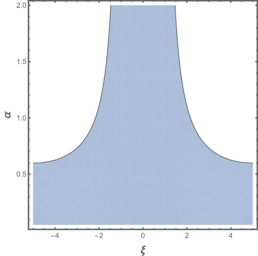
(a) $A=1$

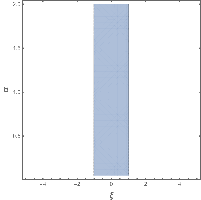
(b) $A=\frac{1}{\sqrt{2}}$

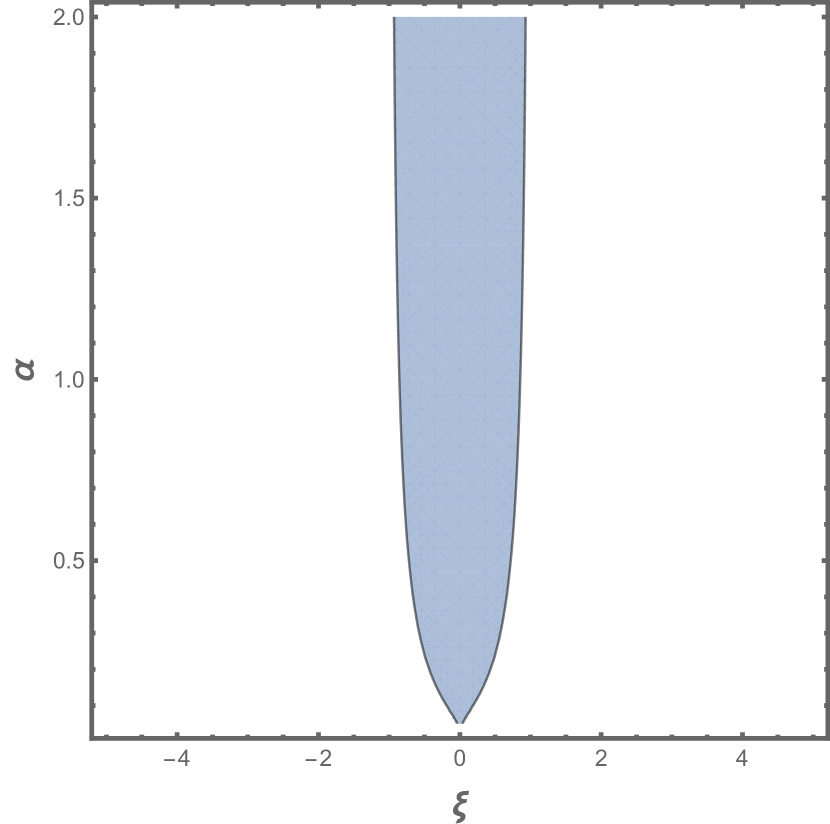
(c) $A=0.5$

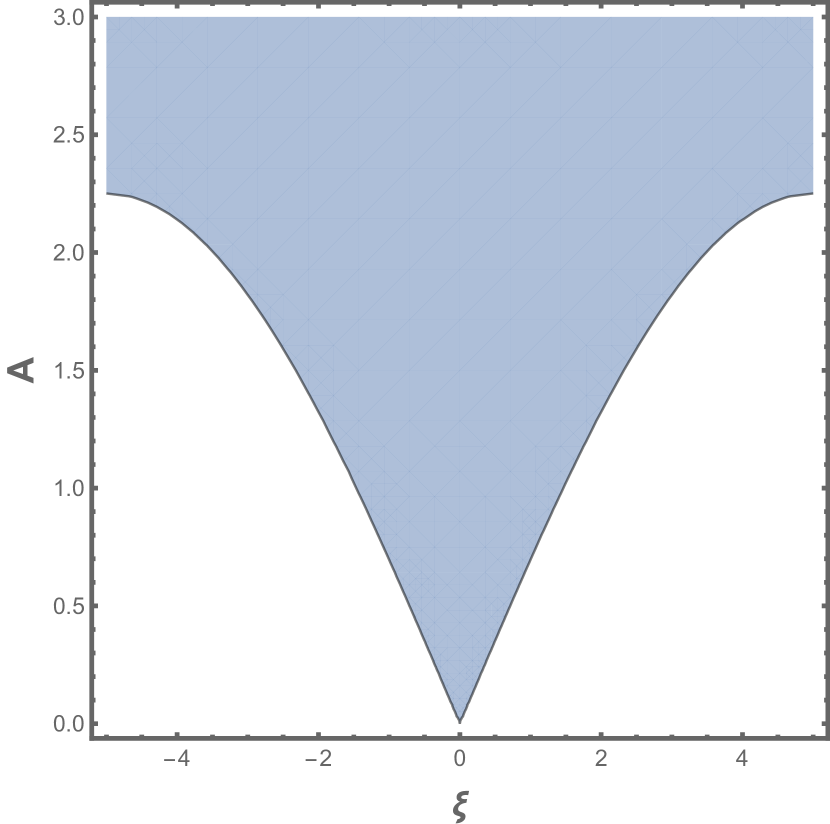
(d) $\alpha=2$

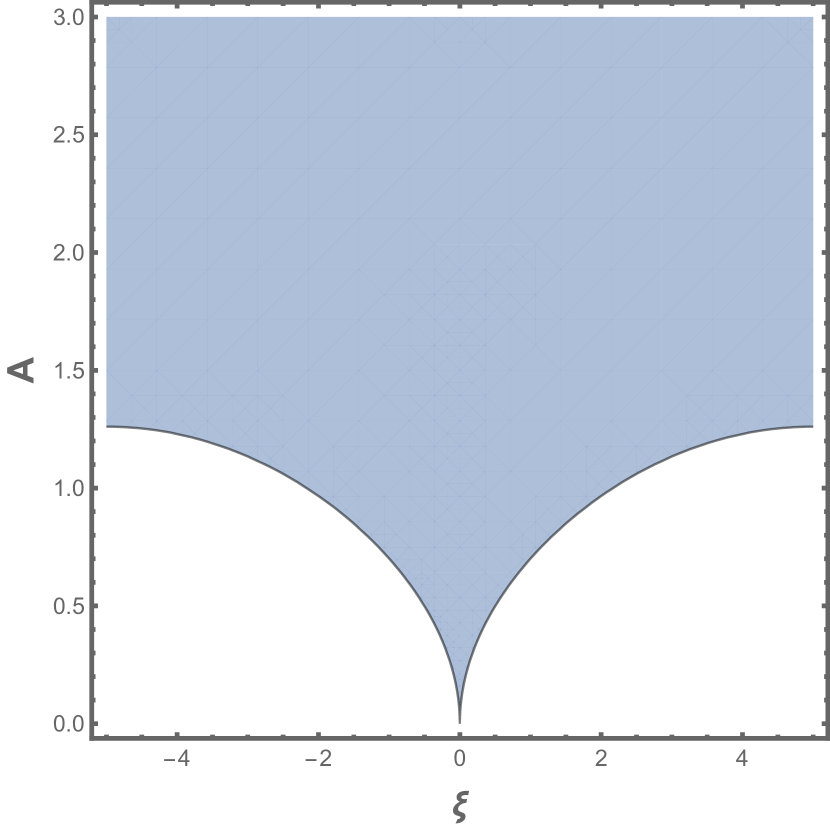
(e) $\alpha=1$

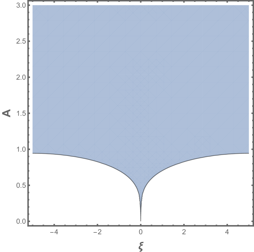
(f) $\alpha=0.5$

Figure 1: The region of linear instability given by (3.3) (in blue) is plotted in $(\xi,A)$ and $(\xi,\alpha)$ for $h=\frac{\pi}{5}$.

Define $u_{h}^{cw}=Ae^{-i\mu|A|^{2}t}$ and let $u_{h}=(A+\epsilon v_{h}(x,t))e^{-i\mu|A|^{2}t}$ where $v_{h}(x,t)\in\mathbb{C},\ |\epsilon|\ll 1$, and $A\in\mathbb{R}$ without loss of generality. The $O(\epsilon)$ term yields

$$i\frac{dv_{h}}{dt}=(-\Delta_{h})^{\frac{\alpha}{2}}v_{h}+\mu A^{2}(v_{h}+\overline{v}_{h}).$$

Taking the real and imaginary parts, i.e. $v_{h}=f_{h}+ig_{h}$, we have

$$\frac{d}{dt}\begin{pmatrix}f_{h}\\ g_{h}\end{pmatrix}=\begin{pmatrix}0&(-\Delta_{h})^{\frac{\alpha}{2}}\\ -(-\Delta_{h})^{\frac{\alpha}{2}}-2\mu A^{2}&0\end{pmatrix}\begin{pmatrix}f_{h}\\ g_{h}\end{pmatrix}.$$ (3.1)

Taking the discrete Fourier transform both sides and the ansatz $\mathcal{F}_{h}[f_{h}]=P_{h}(k)e^{-i\Omega t},\ \mathcal{F}_{h}[g_{h}]=G_{h}(k)e^{-i\Omega t}$, (3.1) becomes an eigenvalue problem whose nontrivial solution $(P_{h},G_{h})$ exists if and only if $\Omega$ satisfies the dispersion relation given by

$$\Omega^{2}(k)=\left|\frac{2}{h}\sin(\frac{hk}{2})\right|^{\alpha}\left(\left|\frac{2}{h}\sin(\frac{hk}{2})\right|^{\alpha}+2\mu A^{2}\right).$$ (3.2)

When $\mu=1$, the system is linearly stable since $\Omega^{2}\geq 0$ and henceforth assume $\mu=-1$. The region of linear instability and the corresponding gain spectrum are given by

$$\left|\frac{2}{h}\sin(\frac{hk}{2})\right|^{\alpha} <2A^{2},\ |k|\leq\frac{\pi}{h},$$ (3.3)

$$G(\xi,A,\alpha,h) :=\sqrt{\left|\frac{2}{h}\sin(\frac{h\xi}{2})\right|^{\alpha}\left(2A^{2}-\left|\frac{2}{h}\sin(\frac{h\xi}{2})\right|^{\alpha}\right)},$$

where we denote $\xi\in\mathbb{R},\ k\in\mathbb{Z}$.

See Figure 1 that illustrates (3.3). Top row: when $A=\frac{1}{\sqrt{2}}$, the region is independent of $\alpha$. If $A\ll 1$ and $\alpha\ll 1$, then there exist no $k\in\mathbb{Z}\setminus\{0\}$ that satisfies (3.3), i.e., linear stability. On the other hand, for $A>\frac{1}{\sqrt{2}}$ and $\alpha\ll 1$, any $k\in\mathbb{T}_{h}$ satisfies (3.3), i.e., linear instability. Botton row: when $\alpha=2$, $A(\xi)$ behaves as a kink and when $\alpha<2$, $A(\xi)$ behaves as a cusp near $\xi=0$. More precisely, $A\sim_{h}\frac{|\xi|^{\frac{\alpha}{2}}}{\sqrt{2}}$ as $\xi\rightarrow 0$. Note that the region approaches $\{|\xi|^{\alpha}<2A^{2}\}$ as $h\rightarrow 0$. Hence for a fixed $h>0$, the system is linearly unstable on the entire bandwidth if $|A|$ is sufficiently large, i.e., if $2A^{2}>(\frac{2}{h})^{\alpha}$.

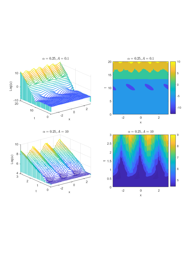
Figure 2: The log plots used $(\alpha,h,k)=(0.25,\frac{\pi}{50},3)$ and $u_{0}(x)=A+10^{-5}e^{ikx}$ where the right plot is the contour of the left plot.

If (3.3) holds, then the maximum exponential gain $\Omega_{m}$ that occurs at $k_{m}$, the fastest-growth frequency, can be computed explicitly by computing the derivative of (3.2) treating $k$ as real. By direct computation, for $\xi\in(0,\frac{\pi}{h})$,

$$\frac{d}{d\xi}\Omega^{2}(\xi)=\alpha h\cot(\frac{h\xi}{2})\left(\frac{2}{h}\sin(\frac{h\xi}{2})\right)^{\alpha}\left(\left(\frac{2}{h}\sin(\frac{h\xi}{2})\right)^{\alpha}-A^{2}\right).$$

If $(\frac{2}{h})^{\alpha}\leq A^{2}$, then $k_{m}=\pm M$ and

$$\Omega_{m}=\sqrt{\left(2A^{2}-\left(\frac{2}{h}\right)^{\alpha}\right)\left(\frac{2}{h}\right)^{\alpha}}.$$ (3.4)

If $(\frac{2}{h})^{\alpha}>A^{2}$, let $\xi_{m}\in(0,\frac{\pi}{h})$ be real such that $\left(\frac{2}{h}\sin(\frac{h\xi_{m}}{2})\right)^{\alpha}=A^{2}$, or equivalently, $\xi_{m}=\frac{2}{h}\sin^{-1}\left(\frac{h|A|^{\frac{2}{\alpha}}}{2}\right)$. It can be verified directly that $\pm\xi_{m}$ is the unique frequency that maximizes $-\Omega^{2}$. Therefore $|k_{m}|\in\{\lfloor\xi_{m}\rfloor,\lceil\xi_{m}\rceil\}$ and $\Omega_{m}=\sqrt{-\Omega^{2}(k_{m})}$. Observe that $\Omega_{m}^{\prime}:=\sqrt{-\Omega^{2}(\xi_{m})}=A^{2}$, independent of $h,\alpha$. A couple of remarks follows.

• In the continuum limit, the region of instability is $\{|k|^{\alpha}<2A^{2}\}$. Since $|\sin(z)|<|z|$ when $0<|z|\leq\frac{\pi}{2}$, the region of linear instability for fDNLS strictly contains that of fNLS.

• The system is linearly stable if $|A|\ll 1,\ \alpha\ll 1$, which is in stark contrast to the system posed on $h\mathbb{Z}$ where given any $A>0$, there exists a real $k$ sufficiently small that satisfies (3.3). In Figure 2, the solution is linearly stable when $|A|\ll 1$. However nonlinearity begins to dominate from $t=10$ with the emergence of $k$ troughs where $k=3$ was used in Figure 2. Indeed numerical experiments suggest the perturbation of $\epsilon e^{ikx}$, with $|\epsilon|\ll 1$ and $k\in\mathbb{T}_{h}^{*}$, triggers the emergence of $k$ troughs as the linear stability is supplanted by highly nonlinear wave evolution. For high $A$ value, the system is linearly unstable.

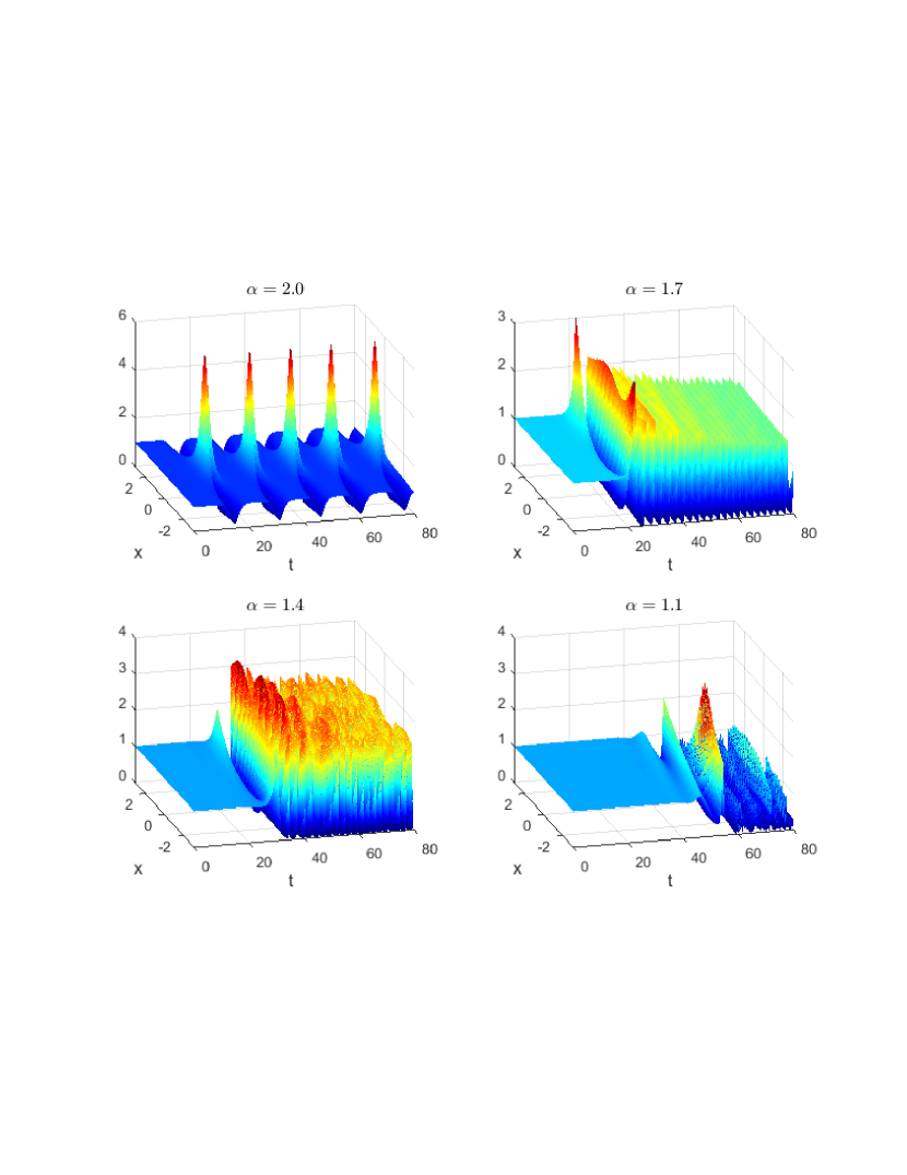
Figure 3: Plots of $|u_{h}(x,t)|^{2}$ with $h=\frac{\pi}{50}$ and $u_{0}(x)=1+10^{-5}(e^{ix}+e^{-ix})$.

• A transition into chaos as $\alpha$ decreases is illustrated in Figure 3, consistent with [29]. For $\alpha=2$, the recurrence of localization was observed as expected; see [13] for a detailed numerical study on the nonlinear evolution of fNLS using the split-step Fourier spectral method. As $\alpha$ decreases to $1$, such clear recurrence was not observed with the development of irregular amplitudes. The time of first localization was observed to be delayed as $\alpha\rightarrow 1+$.

• By (3.4), $\Omega_{m}$ grows linearly in $|A|$ asymptotically as $|A|\rightarrow\infty$ when $h^{-\alpha}\ll A^{2}$. The transition occurs when $h^{-\alpha}\simeq A^{2}$. When $h^{-\alpha}\gg A^{2}$, we have $\Omega_{m}^{\prime}=\sqrt{-\Omega^{2}(\xi_{m})}=A^{2}$; recall that $\xi_{m}$ may not be an integer and that $k_{m}=\lfloor\xi_{m}\rfloor$ or $\lceil\xi_{m}\rceil$. The top plot of Figure 4 reports, for multiple Lévy indices, the initial quadratic growth of $\Omega_{m}$ for sufficiently small $A$, followed by a non-quadratic behavior. The linear stability analysis suggests that the linear growth should follow, consistent with our numerical experiments. However for larger values of $A$, the spectrum of instability for higher harmonics is larger, and therefore the nonlinear evolution seems to be non-negligible.

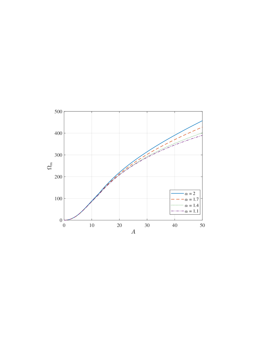
Figure 4: Parameters used for the top plot: $h=\frac{\pi}{50},\ u_{0}(x)=A+10^{-5}e^{50ix}$

4 Strichartz Estimates.

The non-zero curvature of the dispersion relation yields dispersive smoothing estimates, or the Strichartz estimates, manifested as the boundedness of evolution time-dependent operators in various norms of Lebesgue spaces consisting of space-time functions. In [19], the proof of the nonlocal continuum limit in the energy space $H^{\frac{\alpha}{2}}(\mathbb{R})$ when $\alpha\in(1,2)$ is based on the sharp Strichartz estimate

$$\|e^{-it(-\Delta_{h})^{\frac{\alpha}{2}}}f\|_{L^{q}_{t}(\mathbb{R};L^{r}_{h})}\lesssim\||\nabla_{h}|^{\frac{3-\alpha}{q}}f\|_{L^{2}_{h}},$$ (4.1)

for $2\leq q,r\leq\infty$ satisfying $\frac{3}{q}+\frac{1}{r}=\frac{1}{2}$. Since the approach taken to obtain (4.1) does not translate directly to a compact domain, an alternative approach based on approximating an oscillatory sum with an oscillatory integral (Lemma 4.1) was used in [17, 35]. Here we adopt their method and show (Corollary 4.1)

$$\|e^{-it(-\Delta_{h})^{\frac{\alpha}{2}}}f\|_{L^{q}([0,1];L^{r}_{h})}\lesssim_{\epsilon}\|f\|_{H^{\frac{2}{q}+\epsilon}_{h}}.$$ (4.2)

For $f\in L^{1}_{h}\setminus\{0\}$, $\|U_{h}(t)f\|_{L^{\infty}_{h}}$ cannot decay to zero as $t\rightarrow\infty$ due to the conservation of $L^{2}_{h}$ norm; see Proposition 4.2. However the discrete dispersive estimates hold locally in time.

Proposition 4.1.

Let $\alpha\in(1,2]$ and $|t|\leq\frac{\pi^{2-\alpha}}{2\alpha}\left(\frac{h}{N}\right)^{\alpha-1}$. Then

$$\|U_{h}(t)P_{\leq N}f\|_{L^{\infty}_{h}}\lesssim|\alpha-1|^{-\frac{1}{3}}\left(\frac{N}{h}\right)^{1-\frac{\alpha}{3}}|t|^{-\frac{1}{3}}\|f\|_{L^{1}_{h}}.$$ (4.3)

Our proof of Proposition 4.1 is motivated from [17, 35] where a discrete oscillatory sum (see (4.4)) is approximated by an oscillatory integral, after which the Van der Corput Lemma is applied.

Lemma 4.1 ([39, Chapter 5, Lemma 4.4]).

Let $a<b$ and $0<\epsilon<1$. Assume $\sup\limits_{\xi\in(a,b)}|\phi^{\prime}(\xi)|\leq 2\pi(1-\epsilon)$ and $\phi$, monotonic in $(a,b)$. Then there exists $A_{\epsilon}>0$ independent of $a,b,\phi$ such that

$$\left|\int_{a}^{b}e^{i\phi(\xi)}d\xi-\sum_{a<k\leq b}e^{i\phi(k)}\right|\leq A_{\epsilon}.$$

Proof of Proposition 4.1.

Consider the identity

$$\begin{split}U_{h}(t)P_{\leq N}f(x)&=\frac{1}{2\pi}\sum_{|k|\leq\frac{\pi N}{h}}e^{i\left(-t\left|\frac{2}{h}\sin\frac{hk}{2}\right|^{\alpha}+kx\right)}\mathcal{F}_{h}f(k)\\ &=h\sum_{x^{\prime}\in\mathbb{T}_{h}}f(x^{\prime})\sum_{|k|\leq\frac{\pi N}{h}}\frac{1}{2\pi}e^{i\left(-t\left|\frac{2}{h}\sin\frac{hk}{2}\right|^{\alpha}+k(x-x^{\prime})\right)}=K_{t}\ast f,\end{split}$$

where $K_{t}(x):=\sum\limits_{|k|\leq\frac{\pi N}{h}}\frac{1}{2\pi}e^{i\left(-t\left|\frac{2}{h}\sin\frac{hk}{2}\right|^{\alpha}+kx\right)}$ and $\ast$ denotes the discrete convolution defined by the measure $d\mu_{h}$. As a shorthand, let $\phi(\xi)=-t\left|\frac{2}{h}\sin\frac{h\xi}{2}\right|^{\alpha}+\xi x$. It suffices to show

$$\|K_{t}\|_{L^{\infty}_{h}}\lesssim|\alpha-1|^{-\frac{1}{3}}\left(\frac{N}{h}\right)^{1-\frac{\alpha}{3}}|t|^{-\frac{1}{3}}$$ (4.4)

by the Young’s inequality. By the triangle inequality,

$$|K_{t}(x)|\leq\left|K_{t}(x)-\frac{1}{2\pi}\int_{-\frac{\pi N}{h}}^{\frac{\pi N}{h}}e^{i\phi(\xi)}d\xi\right|+\left|\frac{1}{2\pi}\int_{-\frac{\pi N}{h}}^{\frac{\pi N}{h}}e^{i\phi(\xi)}d\xi\right|=:I+II.$$ (4.5)

To show that $I=O(1)$ and $II$ is consistent with (4.4) by Lemma 4.1 and the Van der Corput Lemma, respectively, the higher order derivatives of $\phi$ need to estimated. Let $sgn(\xi)=1$ if $\xi>0$ and $sgn(\xi)=-1$ if $\xi<0$. Then,

$$\begin{split}\phi^{\prime}(\xi)&=-\alpha t\cdot sgn(\xi)\cos\left(\frac{h\xi}{2}\right)\left|\frac{\sin(\frac{h\xi}{2})}{h/2}\right|^{\alpha-1}+x,\\ \phi^{\prime\prime}(\xi)&=\alpha t\left(\frac{h}{2}\right)^{2-\alpha}\frac{1-\alpha\cos^{2}\left(\frac{h\xi}{2}\right)}{\left|\sin\left(\frac{h\xi}{2}\right)\right|^{2-\alpha}},\\ \phi^{\prime\prime\prime}(\xi)&=-\alpha t\left(\frac{h}{2}\right)^{3-\alpha}sgn(\xi)\frac{\left(\alpha^{2}\cos^{2}\left(\frac{h\xi}{2}\right)-3\alpha+2\right)\cos\left(\frac{h\xi}{2}\right)}{\left|\sin\left(\frac{h\xi}{2}\right)\right|^{3-\alpha}}.\end{split}$$ (4.6)

By direct computation, $\phi^{\prime}$ is monotonic on $E_{1}:=(-\xi_{0},\xi_{0})$ and $E_{2}:=[-\frac{\pi}{h},\frac{\pi}{h}]\setminus(-\xi_{0},\xi_{0})$ separately where $\xi_{0}:=\frac{2}{h}\arccos(\alpha^{-\frac{1}{2}})$ is the unique positive root of $\phi^{\prime\prime}$ in $(0,\frac{\pi}{h})$. By choosing $\epsilon=\frac{1}{4}$ in Lemma 4.1, it can further be verified that $\sup\limits_{\xi\in[-\frac{\pi N}{h},\frac{\pi N}{h}]}|\phi^{\prime}(\xi)|\leq\frac{3\pi}{2}$ given the restriction on $|t|$, which shows $I=O(1)$ estimating the difference on $E_{1},E_{2}$ separately.

To estimate the integral in $II$, the lower bounds of $|\phi^{\prime\prime}|,|\phi^{\prime\prime\prime}|$ are estimated. Let

$$S=\Bigl{\{}|\xi|\leq\frac{\pi N}{h}:\left|1-\alpha\cos^{2}\left(\frac{h\xi}{2}\right)\right|\geq\frac{|\alpha-1|}{2}\Bigr{\}}.$$

On $S$, the bound $\left|\sin\left(\frac{h\xi}{2}\right)\right|\leq\frac{h|\xi|}{2}$ is used to obtain

$$|\phi^{\prime\prime}(\xi)|\gtrsim(\alpha-1)|t||\xi|^{-(2-\alpha)}.$$ (4.7)

On $[-\frac{\pi N}{h},\frac{\pi N}{h}]\setminus S$, we have

$$|\phi^{\prime\prime\prime}(\xi)|\gtrsim(\alpha-1)|t||\xi|^{-(3-\alpha)},$$

since

$$\left|\alpha^{2}\cos^{2}\left(\frac{h\xi}{2}\right)-3\alpha+2\right|\geq 2|\alpha-1|-\left|\alpha^{2}\cos^{2}\left(\frac{h\xi}{2}\right)-\alpha\right|\geq 2|\alpha-1|-\frac{\alpha}{2}|\alpha-1|\geq\alpha-1,$$

and

$$\left|\alpha\cos^{2}\left(\frac{h\xi}{2}\right)\right|\geq 1-\left|\alpha\cos^{2}\left(\frac{h\xi}{2}\right)-1\right|\geq 1-\frac{|\alpha-1|}{2}\geq\frac{1}{2}.$$

Hence

$$\begin{split}\left|\int_{-\frac{\pi N}{h}}^{\frac{\pi N}{h}}e^{i\phi(\xi)}d\xi\right|&\leq\left|\int_{S}e^{i\phi(\xi)}d\xi\right|+\left|\int_{[-\frac{\pi N}{h},\frac{\pi N}{h}]\setminus S}e^{i\phi(\xi)}d\xi\right|\\ &\lesssim\max\left((\alpha-1)^{-\frac{1}{2}}\left(\frac{N}{h}\right)^{1-\frac{\alpha}{2}}|t|^{-\frac{1}{2}},(\alpha-1)^{-\frac{1}{3}}\left(\frac{N}{h}\right)^{1-\frac{\alpha}{3}}|t|^{-\frac{1}{3}}\right)\\ &\lesssim(\alpha-1)^{-\frac{1}{3}}\left(\frac{N}{h}\right)^{1-\frac{\alpha}{3}}|t|^{-\frac{1}{3}},\end{split}$$ (4.8)

where the last inequality follows from interpolating $\left|\int_{-\frac{\pi N}{h}}^{\frac{\pi N}{h}}e^{i\phi(\xi)}d\xi\right|\lesssim\frac{N}{h}$ and the Van der Corput estimate obtained from (4.7). Substituting $I=O(1)$ and (4.8) into (4.5), the desired estimate (4.4) is shown since for $|t|\lesssim(\frac{h}{N})^{\alpha-1}$ and $N\geq N_{*}$,

$$(\alpha-1)^{-\frac{1}{3}}\left(\frac{N}{h}\right)^{1-\frac{\alpha}{3}}|t|^{-\frac{1}{3}}\gtrsim(\alpha-1)^{-\frac{1}{3}}\left(\frac{N}{h}\right)^{\frac{2}{3}}\gtrsim(\alpha-1)^{-\frac{1}{3}}.$$

∎

Corollary 4.1.

Let $(q,r)\in[2,\infty]^{2}$ be lattice-admissible and $\alpha\in(1,2]$. Then for all $\epsilon>0$,

$$\|U_{h}(t)f\|_{L^{q}([0,1];L^{r}_{h})} \lesssim_{\epsilon}|\alpha-1|^{-\frac{1}{6}(1-\frac{2}{r})}\|f\|_{H^{\frac{2}{q}+\epsilon}_{h}},$$ (4.9)

$$\left|\left|\int_{0}^{t}U_{h}(t-t^{\prime})F(t^{\prime})dt^{\prime}\right|\right|_{L^{q}([0,1];L^{r}_{h})} \lesssim_{\epsilon}|\alpha-1|^{-\frac{1}{3}(1-\frac{2}{r})}\|F\|_{L^{1}([0,1];H^{\frac{2}{q}+\epsilon}_{h})}.$$ (4.10)

Proof.

Observe that $\tilde{U}_{h}(t)=P_{\leq N}U_{h}(t(\frac{N}{h})^{3-\alpha})P_{\leq N}$ satisfies the hypothesis of [25, Theorem 1.2], and therefore

$$\|U_{h}(t)P_{\leq N}f\|_{L^{q}([0,\tau];L^{r}_{h})}\lesssim|\alpha-1|^{-\frac{1}{6}(1-\frac{2}{r})}\left(\frac{N}{h}\right)^{\frac{3-\alpha}{q}}\|f\|_{L^{2}_{h}},$$ (4.11)

where $\tau=\frac{\pi^{2-\alpha}}{2\alpha}\left(\frac{h}{N}\right)^{\alpha-1}$. By iterating (4.11) on $[0,1]$ using the unitarity of $U_{h}(t)$, (4.9) is shown. Another application of [25, Theorem 1.2] yields the inhomogeneous estimate (4.10). Note that the implicit constant of (4.10) is that of (4.9) squared by the TT^∗ argument based on the complex interpolation of dispersive estimates between $\|U_{h}(t)P_{\leq N}f\|_{L^{2}_{h}}\leq\|f\|_{L^{2}_{h}}$ and (4.3) given by

$$\|U_{h}(t)P_{\leq N}f\|_{L^{r}_{h}}\lesssim|\alpha-1|^{-\frac{1}{3}(1-\frac{2}{r})}\left(\frac{N}{h}\right)^{(1-\frac{\alpha}{3})(1-\frac{2}{r})}|t|^{-\frac{1}{3}(1-\frac{2}{r})}\|f\|_{L^{\frac{r}{r-1}}_{h}}.$$

∎

Remark 4.1.

Our proof of Proposition 4.1 and Corollary 4.1 is adapted from [17]. The proof of Proposition 4.1 differs from that of [17] in that we use $\epsilon>0$ when applying Lemma 4.1 whereas [17] used $\epsilon=0$, which may lead to the error bound $A_{\epsilon}$ to blow up. This subtlety can be easily circumvented by choosing $0<\epsilon<\frac{1}{2}$. Furthermore note that the right-hand side (RHS) of (4.9) is measured in $H^{\frac{2}{q}+\epsilon}_{h}$ whose Sobolev regularity is independent of $\alpha$. The $\epsilon>0$ is a result of the non-endpoint Sobolev embedding.

The time interval $[0,T]$ of the local well-posedness of (1.1) in the Strichartz space $X_{T}:=C([0,T];L^{2}_{h})\cap L^{6}([0,T];L^{\infty}_{h})$ cannot be determined uniformly in $h>0$ solely from $L^{p}_{h}\hookrightarrow L^{q}_{h}$, for $p<q$, since the embedding is not uniform in $h$ as $\|f\|_{L^{q}_{h}}\leq h^{\frac{1}{p}-\frac{1}{q}}\|f\|_{L^{p}_{h}}$. An application of Corollary 4.1 yields a uniform estimate in $h$.

Proposition 4.2.

Let $s>\frac{1}{3}$ and $\alpha\in(1,2]$. For every $u_{h,0}\in H^{s}_{h}$, there exists a unique $u_{h}\in X_{T}$ such that

$$u_{h}(t)=U_{h}(t)u_{h,0}-i\mu\int_{0}^{t}U_{h}(t-\tau)\left(|u_{h}(\tau)|^{2}u_{h}(\tau)\right)d\tau$$ (4.12)

where $T_{h}\sim_{\alpha}\|u_{h,0}\|_{H^{s}_{h}}^{-3}$ is independent of $h>0$. Furthermore discrete mass ($M_{h}$) and discrete energy ($H_{h}$) are conserved where

$$M_{h}[u_{h}(t)]=\|u_{h}(t)\|_{L^{2}_{h}}^{2};\ H_{h}[u_{h}(t)]=\frac{1}{2}\||\nabla_{h}|^{\frac{\alpha}{2}}u_{h}\|_{L^{2}_{h}}^{2}+\frac{\mu}{4}\|u_{h}\|_{L^{4}_{h}}^{4}.$$

Proof.

Let $\Gamma u_{h}$ be the RHS of (4.12). By Corollary 4.1 and the a priori estimate,

$$\begin{split}\|\Gamma u_{h}\|_{X_{T}}&:=\|\Gamma u_{h}\|_{C_{T}H^{s}_{h}}+\|\Gamma u_{h}\|_{L^{6}_{T}L^{\infty}_{h}}\lesssim\|u_{h,0}\|_{H^{s}_{h}}+\||u_{h}|^{2}u_{h}\|_{L^{1}_{T}H^{s}_{h}}\\ &\lesssim\|u_{h,0}\|_{H^{s}_{h}}+\left|\left|\|u_{h}\|_{L^{\infty}_{h}}^{2}\|u_{h}\|_{H^{s}_{h}}\right|\right|_{L^{1}_{T}}\leq\|u_{h,0}\|_{H^{s}_{h}}+T^{\frac{2}{3}}\|u_{h}\|_{L^{6}_{T}L^{\infty}_{h}}^{2}\|u_{h}\|_{C_{T}H^{s}_{h}},\\ \|\Gamma u_{h}-\Gamma v_{h}\|_{X_{T}}&\lesssim T^{\frac{2}{3}}(\|u_{h}\|_{X_{T}}^{2}+\|v_{h}\|_{X_{T}}^{2})\|u_{h}-v_{h}\|_{X_{T}},\end{split}$$

there exists a unique fixed point $u_{h}$ in a small closed ball of $X_{T}$ such that $u_{h}=\Gamma u_{h}$. The domain of $\Gamma$ is extended from the neighborhood of the origin to the entire $X_{T}$ by the continuity argument. ∎

5 Convergence as $h\rightarrow 0$.

The proof of (1.2) is presented. Our strategy is to directly estimate the difference, or the error, between the solutions on $\mathbb{T}$ and $\mathbb{T}_{h}$. To address the subtlety that $u(t)$ and $u_{h}(t)$ are defined on different spaces, we lift $u_{h}(t)$ via linear interpolation. Since there is no canonical way to interpolate discrete data into continuum data or vice versa via discretization, there is flexibility in how the error is defined and computed. For example, the exact solution whose spatiotemporal frequency is concentrated at a single site admits linear convergence (B) in $L^{2}(\mathbb{T})$ and quadratic convergence (5.3) in $L^{2}_{h}$. Whether or not other methods of error estimation yield similar results as Theorem 1.1 is left for further research.

The technical lemmas used to prove the theorem are adapted from [19, 17] either directly or with minimal modifications.

Lemma 5.1.

Let $0\leq s\leq 1$. Then

$$\|p_{h}U_{h}(t)u_{h,0}-U(t)u_{0}\|_{L^{2}(\mathbb{T})}\lesssim|t|h^{\frac{s}{1+s}}(\|u_{h,0}\|_{H^{s}_{h}}+\|u_{0}\|_{H^{s}(\mathbb{T})})+\|p_{h}u_{h,0}-u_{0}\|_{L^{2}(\mathbb{T})}.$$

Lemma 5.2.

For $0\leq s\leq 1,\ 0\leq\tau\leq t$,

$$\|(p_{h}U_{h}(t-\tau)-U(t-\tau)p_{h})F(\tau)\|_{L^{2}(\mathbb{T})}\lesssim|t-\tau|h^{\frac{s}{1+s}}\|F(\tau)\|_{H^{s}_{h}(\mathbb{T})}.$$

Lemma 5.3.

For $p>1,\ 0<s\leq 1$,

$$\|p_{h}(|u_{h}|^{p-1}u_{h})-|p_{h}u_{h}|^{p-1}p_{h}u_{h}\|_{L^{2}(\mathbb{T})}\lesssim h^{s}\|u_{h}\|_{L^{\infty}_{h}}^{p-1}\|u_{h}\|_{H^{s}_{h}}.$$

Lemma 5.4.

For $0\leq s\leq 1$,

$$\|p_{h}d_{h}f-f\|_{L^{2}(\mathbb{T})}\lesssim h^{s}\|f\|_{H^{s}(\mathbb{T})}.$$

Proof of (1.2).

In this proof, $\|\cdot\|$ denotes the norm in $L^{2}(\mathbb{T})$. Given $u_{0}\in H^{s}(\mathbb{T})$, let $u(t)=S(t)u_{0}$ and $u_{h}(t)=S_{h}(t)d_{h}u_{0}$. It can be directly verified that $d_{h}$ defines a bounded linear operator from $L^{2}(\mathbb{T})$ to $L^{2}_{h}$ and $H^{1}(\mathbb{T})$ to $H^{1}_{h}$, and consequently it follows from interpolating the two estimates that $d_{h}:H^{s^{\prime}}(\mathbb{T})\rightarrow H^{s^{\prime}}_{h}$ is bounded for any $s^{\prime}\in[0,1]$. Therefore the time of existence in Proposition 4.2 is bounded from below since $T_{h}\sim_{\alpha}\|d_{h}u_{0}\|_{H^{s}_{h}}^{-3}\gtrsim\|u_{0}\|_{H^{s}}^{-3}$. Let $T^{\prime}(\|u_{0}\|_{H^{s}})>0$ be the time of existence stated in Proposition A.1 and take

$$T:=\min\{T^{\prime},\inf\limits_{h}T_{h}\}>0.$$ (5.1)

By the triangle inequality and Lemma 5.1, Lemma 5.2, and Lemma 5.3, we have

$$\|(p_{h}S_{h}(t)d_{h}-S(t))u_{0}\| \leq\|(p_{h}U_{h}(t)d_{h}-U(t))u_{0}\|+\int_{0}^{t}\|(p_{h}U_{h}(t-\tau)-U(t-\tau)p_{h})(|u_{h}|^{2}u_{h})(\tau)\|d\tau$$

$$+\int_{0}^{t}\|p_{h}(|u_{h}|^{2}u_{h})-|p_{h}u_{h}|^{2}p_{h}u_{h}\|d\tau+\int_{0}^{t}\||p_{h}u_{h}|^{2}p_{h}u_{h}-|u|^{2}u\|d\tau$$

$$=:I_{1}+I_{2}+I_{3}+I_{4}$$ (5.2)

$$\lesssim(1+|T|)h^{\frac{s}{1+s}}\|u_{0}\|_{H^{s}_{h}} +\int_{0}^{t}(|t-\tau|h^{\frac{s}{1+s}}+h^{s})\|u_{h}\|_{L^{\infty}_{h}}^{2}\|u_{h}\|_{H^{s}_{h}}d\tau+\int_{0}^{t}(\|p_{h}u_{h}\|_{L^{\infty}}^{2}+\|u\|_{L^{\infty}}^{2})\|p_{h}u_{h}-u\|d\tau,$$ (5.3)

having used the discrete Sobolev estimate $\||u_{h}|^{2}u_{h}\|_{H^{s}_{h}}\lesssim\|u_{h}\|_{L^{\infty}}^{2}\|u_{h}\|_{H^{s}_{h}}$. Similar to the proof of Proposition 4.2 where $X_{T}=C([0,T_{h}];L^{2}_{h})\cap L^{6}([0,T_{h}];L^{\infty}_{h})$, the nonlinear terms are estimated as

$$\left|\left|\|u_{h}\|_{L^{\infty}_{h}}^{2}\|u_{h}\|_{H^{s}_{h}}\right|\right|_{L^{1}_{T}}\leq T_{h}^{\frac{2}{3}}\|u_{h}\|_{X_{T}}^{3}\lesssim\|d_{h}u_{0}\|_{H^{s}_{h}}\lesssim\|u_{0}\|_{H^{s}}.$$

Furthermore a direct estimation on the linear interpolation yields $\|p_{h}u_{h}\|_{L^{\infty}}\lesssim\|u_{h}\|_{L^{\infty}_{h}}$ since for $x_{0}\in\mathbb{T}_{h}$ and $x\in[x_{0},x_{0}+h)$,

$$|p_{h}u_{h}(x)|\leq|u_{h}(x_{0})|+\frac{|u_{h}(x_{0}+h)|+|u_{h}(x_{0})|}{h}|x-x_{0}|\leq 3\|u_{h}\|_{L^{\infty}_{h}}.$$

Altogether

$$\eqref{estimate1}\lesssim(1+|T|)h^{\frac{s}{1+s}}\|u_{0}\|_{H^{s}_{h}}+\int_{0}^{t}(\|u_{h}\|_{L^{\infty}_{h}}^{2}+\|u\|_{L^{\infty}}^{2})\|p_{h}u_{h}-u\|d\tau,$$

and the Gronwall’s inequality for $t\in[0,T]$ yields

$$\|p_{h}u_{h}(t)-u(t)\|\lesssim(1+|T|)h^{\frac{s}{1+s}}\|u_{0}\|_{H^{s}_{h}}e^{\int_{0}^{T}\|u_{h}(\tau)\|_{L^{\infty}_{h}}^{2}+\|u(\tau)\|_{L^{\infty}}^{2}d\tau}.$$

It suffices to show that there exists $C(\|u_{0}\|_{H^{s}},\alpha)>0$ independent of $h$ such that $\|u_{h}\|_{L^{2}_{T}L^{\infty}_{h}}^{2}+\|u\|_{L^{2}_{T}L^{\infty}}^{2}\leq C$. By Proposition 4.2,

$$\|u_{h}\|_{L^{2}_{T}L^{\infty}_{h}}^{2}\leq T_{h}^{\frac{2}{3}}\|u_{h}\|_{X_{T}}^{2}=O(1)$$

is independent of $h$. To show $\|u\|_{L^{2}_{T}L^{\infty}}^{2}=O(1)$, note that

$$\|u\|_{L^{2}_{T}L^{\infty}}^{2}\leq T^{\frac{1}{2}}\|u\|_{L^{4}_{T}L^{\infty}}^{2}\lesssim T^{\frac{1}{2}}\|u\|_{L^{4}_{T}W^{\frac{1}{4}+\epsilon^{\prime},4}}^{2},$$ (5.4)

by the Hölder’s inequality and the Sobolev embedding $W^{\frac{1}{4}+\epsilon^{\prime},4}(\mathbb{T})\hookrightarrow L^{\infty}(\mathbb{T})$ where $0<\epsilon^{\prime}<s-\frac{3-\alpha}{4}$. Then Proposition A.2 is applied at the minimum regularity $\frac{2-\alpha}{4}$ and $0<\epsilon\ll 1$ to obtain

$$\eqref{estimate3}\lesssim T^{\frac{1}{2}}\|u\|_{X_{T}^{\frac{1}{4}+\epsilon^{\prime},\frac{1}{2}-\epsilon}}\|u\|_{X_{T}^{\frac{3-\alpha}{4}+\epsilon^{\prime},\frac{1}{2}+\epsilon}}\lesssim T^{\frac{1}{2}}\|u\|_{X_{T}^{\frac{3-\alpha}{4}+\epsilon^{\prime},\frac{1}{2}+\epsilon}}^{2}\lesssim T^{\frac{1}{2}}\|u\|_{C_{T}H^{s}}^{2}\lesssim T^{\frac{1}{2}}\|u_{0}\|_{H^{s}}^{2},$$

where the second and the third estimates reflect the embeddings $X_{T}^{s_{1},b_{1}}\hookrightarrow X_{T}^{s_{2},b_{2}}$, for $s_{1}\geq s_{2},\ b_{1}\geq b_{2}$, and $X_{T}^{s,\frac{1}{2}+\epsilon}\hookrightarrow C([0,T];H^{s}(\mathbb{T}))$, respectively, and the last inequality follows from the proof of Proposition A.1 based on the fixed point argument. ∎

Remark 5.1.

Since there is no canonical way to define a numerical error, the convergence rate depends on the method of discretization and interpolation. As (2.1), we discretize data on a smooth domain by averaging over an interval of length $h$ and linearly interpolate discrete data. Though we do not take the following approach, [2, 6] considered the pointwise projection of continuous functions onto $h\mathbb{Z}$ and the Shannon interpolation that takes the discrete convolution of discrete data against the sinc function. It is commented in [6] that the Shannon interpolation is better suited to show convergence in higher Sobolev norms. It is of interest to show the continuum limit of our model in higher Sobolev norms, which would require a uniform-in-$h$ control of the Sobolev norms of discrete solutions. However the method of modified energy used in the previous references to obtain bounds on higher Sobolev norms is not directly applicable in our nonlocal case due to the complexity of the Leibniz rule for fractional derivatives.

Now we show the sharpness of the convergence rate of the continuum limit at the energy space $H^{\frac{\alpha}{2}}(\mathbb{T})$. The mass and energy conservation for sufficiently regular data admits the global result.

Proposition 5.1.

Let $\alpha\in(1,2]$ and $u_{0}\in H^{\frac{\alpha}{2}}(\mathbb{T})$. Then there exists $C_{1},C_{2}>0$ depending only on $\|u_{0}\|_{H^{\frac{\alpha}{2}}}$ and $\alpha$ such that the error estimate

$$\|p_{h}S_{h}(t)d_{h}u_{0}-S(t)u_{0}\|_{L^{2}(\mathbb{T})}\leq C_{1}h^{\frac{\alpha}{2+\alpha}}e^{C_{2}|t|}(1+\|u_{0}\|_{H^{\frac{\alpha}{2}}})^{3},$$ (5.5)

holds for all $t\in\mathbb{R}$.

Proof.

With initial data of finite energy, the Sobolev embedding $H^{\frac{\alpha}{2}}(\mathbb{T})\hookrightarrow L^{\infty}(\mathbb{T})$ allows a more straightforward proof, without resorting to the Strichartz estimates, than the one presented in Section 5. ∎

It is of interest to show the existence of $u_{0}\in H^{\frac{\alpha}{2}}(\mathbb{T})$ such that

$$C_{1}(t,\|u_{0}\|_{H^{\frac{\alpha}{2}}})h^{\frac{2}{2+\alpha}}\leq\|p_{h}S_{h}(t)d_{h}u_{0}-S(t)u_{0}\|_{L^{2}}\leq C_{2}(t,\|u_{0}\|_{H^{\frac{\alpha}{2}}})h^{\frac{2}{2+\alpha}},$$

for any $t\in\mathbb{R}$. Instead we derive a partial result that is local in time, which shows the sharpness of the convergence rate $\frac{\alpha}{2+\alpha}$ in (5.5).

Proposition 5.2.

Let $\alpha\in(1,2]$. There exists $0<T\ll 1$ such that for any $0<h\ll 1$, we have $u_{0}^{h}\in H^{\frac{\alpha}{2}}(\mathbb{T})$ with $\|u_{0}^{h}\|_{H^{\frac{\alpha}{2}}}=O(1)$, independent of $h$, satisfying

$$\|p_{h}S_{h}(t)d_{h}u_{0}^{h}-S(t)u_{0}^{h}\|_{L^{\infty}_{T}L^{2}}\geq c(T,\alpha)h^{\frac{2}{2+\alpha}},$$

where $c>0$ is independent of $h>0$.

Proof.

We fix $\alpha$ once and for all and all constants resulting from the Sobolev embedding or the Strichartz estimates are considered as implicit constants. Fix $T>0$ as (5.1) corresponding to $\{u_{0}:\|u_{0}\|_{H^{\frac{\alpha}{2}}}=O(1)\}$. Recall from the proof of Proposition 4.2 that $\|u_{h}\|_{L^{\infty}_{T}H^{\frac{\alpha}{2}}}\lesssim\|d_{h}u_{0}\|_{H_{h}^{\frac{\alpha}{2}}}$ where an explicit description of $u_{0}$ is given in (5.12). Let $t\in[0,T]$ and $h\ll_{\alpha}1$. From (5.2),

$$\begin{split}I_{2}(t)+I_{3}(t)&\lesssim\int_{0}^{t}(|t-\tau|h^{\frac{\alpha}{2+\alpha}}+h^{\frac{\alpha}{2}})\|u_{h}\|_{L^{\infty}_{h}}^{2}\|u_{h}\|_{H_{h}^{\frac{\alpha}{2}}}d\tau\lesssim\|u_{h}\|^{3}_{L^{\infty}_{T}H_{h}^{\frac{\alpha}{2}}}\int_{0}^{t}(|t-\tau|h^{\frac{\alpha}{2+\alpha}}+h^{\frac{\alpha}{2}})d\tau\\ &\lesssim\|d_{h}u_{0}\|_{H^{\frac{\alpha}{2}}_{h}}^{3}(t^{2}h^{\frac{\alpha}{2+\alpha}}+|t|h^{\frac{\alpha}{2}})\lesssim\|u_{0}\|_{H^{\frac{\alpha}{2}}}^{3}Th^{\frac{\alpha}{2+\alpha}},\end{split}$$

where we shrink $T$, if necessary, to admit the last inequality. On the other,

$$\begin{split}\int_{0}^{t}(\|p_{h}u_{h}\|_{L^{\infty}}^{2}+\|u\|_{L^{\infty}}^{2})\|p_{h}u_{h}-u\|d\tau&\leq(\|p_{h}u_{h}\|_{L^{2}([0,t];L^{\infty})}^{2}+\|u\|_{L^{2}([0,t];L^{\infty})}^{2})\|p_{h}u_{h}-u\|_{L^{\infty}([0,t];L^{2})}\\ &\lesssim\|p_{h}u_{h}-u\|_{L^{\infty}_{T}L^{2}},\end{split}$$

since $\|p_{h}u_{h}\|_{L^{2}([0,t];L^{\infty})}^{2}+\|u\|_{L^{2}([0,t];L^{\infty})}^{2}=O(1)$ as in the proof of Theorem 1.1. Hence by the triangle inequality, we have

$$\|p_{h}S_{h}(\cdot)d_{h}u_{0}-S(\cdot)u_{0}\|_{L^{\infty}_{T}L^{2}}\gtrsim\|p_{h}U_{h}(t)d_{h}u_{0}-U(t)u_{0}\|_{L^{2}}-\|u_{0}\|_{H^{\frac{\alpha}{2}}}^{3}Th^{\frac{\alpha}{2+\alpha}}.$$ (5.6)

Observe that

$$\|p_{h}U_{h}(t)d_{h}u_{0}-U(t)u_{0}\|_{L^{2}}\geq\|p_{h}U_{h}(t)d_{h}u_{0}-U(t)p_{h}d_{h}u_{0}\|_{L^{2}}-\|U(t)(p_{h}d_{h}u_{0}-u_{0})\|_{L^{2}}=:A_{1}-A_{2},$$ (5.7)

where $A_{2}\lesssim h^{\frac{\alpha}{2}}\|u_{0}\|_{H^{\frac{\alpha}{2}}}$ by the unitarity of $U(t)$ and Lemma 5.4. By the Plancherel’s Theorem,

$$\sqrt{2\pi}A_{1} =\|(e^{-it\left|\frac{2}{h}\sin\frac{hk}{2}\right|^{\alpha}}-e^{-it|k|^{\alpha}})\mathcal{F}[p_{h}d_{h}u_{0}]\|_{l^{2}}$$

$$\geq\|(e^{-it\left|\frac{2}{h}\sin\frac{hk}{2}\right|^{\alpha}}-e^{-it|k|^{\alpha}})\widehat{u}_{0}\|_{l^{2}}-\|(e^{-it\left|\frac{2}{h}\sin\frac{hk}{2}\right|^{\alpha}}-e^{-it|k|^{\alpha}})(\mathcal{F}[p_{h}d_{h}u_{0}]-\widehat{u}_{0})\|_{l^{2}}$$

$$\geq\|(e^{-it\left|\frac{2}{h}\sin\frac{hk}{2}\right|^{\alpha}}-e^{-it|k|^{\alpha}})\widehat{u}_{0}\|_{l^{2}}-Ch^{\frac{\alpha}{2}}\|u_{0}\|_{H^{\frac{\alpha}{2}}},$$ (5.8)

where $C>0$ is by Lemma 5.4. The lower bound of the phase difference is estimated. By direct computation,

$$\left|e^{-it\left|\frac{2}{h}\sin\frac{hk}{2}\right|^{\alpha}}-e^{-it|k|^{\alpha}}\right|=2\left|\sin\left(\frac{2^{\alpha}t}{h^{\alpha}}\left(\left|\sin\frac{hk}{2}\right|^{\alpha}-\left|\frac{hk}{2}\right|^{\alpha}\right)\right)\right|.$$

For $|k|\leq(10h)^{-1}$, the Taylor expansion yields the alternating series

$$\left|\sin\frac{hk}{2}\right|^{\alpha}-\left|\frac{hk}{2}\right|^{\alpha}=\left|\frac{hk}{2}\right|^{\alpha}\left(-\frac{\alpha}{24}(hk)^{2}+\frac{\alpha(5\alpha-2)}{5760}(hk)^{4}-O_{\alpha}((hk)^{4}))\right),$$ (5.9)

and therefore

$$\frac{2^{\alpha}|t|}{h^{\alpha}}\cdot\left|\left|\sin\frac{hk}{2}\right|^{\alpha}-\left|\frac{hk}{2}\right|^{\alpha}\right|\leq\frac{\alpha|t|}{24}h^{2}|k|^{2+\alpha}.$$ (5.10)

To apply the lower bound estimate

$$|\sin\theta|\geq\frac{2}{\pi}|\theta|,\ \text{for any\ }|\theta|\leq\frac{\pi}{2},$$

let $\theta=\frac{2^{\alpha}t}{h^{\alpha}}\left(\left|\sin\frac{hk}{2}\right|^{\alpha}-\left|\frac{hk}{2}\right|^{\alpha}\right)$ and by (5.10), assume that $E$ holds where

$$E=\{k\in\mathbb{Z}:|k|\leq\left(\frac{12\pi}{\alpha}\right)^{\frac{1}{2+\alpha}}|t|^{-\frac{1}{2+\alpha}}h^{-\frac{2}{2+\alpha}}\}.$$

Then by the trigonometric lower bound estimate and (5.9),

$$\left|e^{-it\left|\frac{2}{h}\sin\frac{hk}{2}\right|^{\alpha}}-e^{-it|k|^{\alpha}}\right|\geq\frac{2^{2+\alpha}|t|}{\pi h^{\alpha}}\cdot\left|\left|\sin\frac{hk}{2}\right|^{\alpha}-\left|\frac{hk}{2}\right|^{\alpha}\right|\geq\frac{\alpha|t|}{12\pi}h^{2}|k|^{2+\alpha},$$

and using this lower bound estimate, we have

$$\|(e^{-it\left|\frac{2}{h}\sin\frac{hk}{2}\right|^{\alpha}}-e^{-it|k|^{\alpha}})\widehat{u}_{0}\|_{l^{2}}\geq\|(e^{-it\left|\frac{2}{h}\sin\frac{hk}{2}\right|^{\alpha}}-e^{-it|k|^{\alpha}})\widehat{u}_{0}\|_{l^{2}(E)}\gtrsim|t|h^{2}\||k|^{2+\alpha}\widehat{u}_{0}\|_{l^{2}(E)}.$$ (5.11)

Let $k_{0}=|t|^{-\frac{1}{2+\alpha}}h^{-\frac{2}{2+\alpha}}$. For $\epsilon>0$ to be determined below, define

$$\widehat{u}_{0}^{h}(k)=\epsilon k_{0}^{-\frac{\alpha}{2}}\delta_{k_{0}}(k)$$ (5.12)

where $\delta_{k_{0}}$ is the Kronecker delta function supported at $k=k_{0}$. Hence by (5.6), (5.7), (5), and (5.11),

$$\begin{split}\|p_{h}S_{h}(\cdot)d_{h}u_{0}^{h}-S(\cdot)u_{0}^{h}\|_{L^{\infty}_{T}L^{2}}&\gtrsim Th^{2}\||k|^{2+\alpha}\widehat{u}^{h}_{0}\|_{l^{2}(E)}-\|u_{0}^{h}\|_{H^{\frac{\alpha}{2}}}^{3}Th^{\frac{\alpha}{2+\alpha}}-\|u_{0}^{h}\|_{H^{\frac{\alpha}{2}}}h^{\frac{\alpha}{2}}\\ &\simeq(\epsilon T^{\frac{\alpha/2}{2+\alpha}}-\epsilon^{3}T)h^{\frac{\alpha}{2+\alpha}}-\epsilon h^{\frac{\alpha}{2}}\\ &\gtrsim(\frac{\epsilon}{2}-\epsilon^{3})T^{\frac{\alpha/2}{2+\alpha}}h^{\frac{\alpha}{2+\alpha}},\end{split}$$

where the last inequality assumes $T\leq 1$ and $h$ sufficiently small depending on $\alpha$ and $T$; for example, $h\leq\left(\frac{T^{\frac{\alpha/2}{2+\alpha}}}{2}\right)^{\frac{4+2\alpha}{\alpha^{2}}}$ would do. The proof is complete by taking $0<\epsilon<\frac{1}{\sqrt{2}}$. ∎

Corollary 5.1.

Let $T>0$ be as Proposition 5.2 and suppose

$$\sup_{\|u_{0}\|_{H^{\frac{\alpha}{2}}(\mathbb{T})}<R}\|p_{h}S_{h}(\cdot)d_{h}u_{0}-S(\cdot)u_{0}\|_{L^{\infty}_{T}L^{2}}\lesssim_{T,R,\alpha}h^{p},$$ (5.13)

for some $R>0,\ p>0$. Then $\max\{p:\eqref{sharpness_cor}\ \text{holds for all\ }h>0\}=\frac{2}{2+\alpha}$.

Proof.

By Proposition 5.1, $\frac{2}{2+\alpha}$ satisfies $\eqref{sharpness_cor}$ for any $R>0$. Any $p>\frac{2}{2+\alpha}$ is not in the desired set by an explicit construction in Proposition 5.2. ∎

Remark 5.2.

The sharpness of the convergence rate is expected to be $O(h^{\frac{s}{1+s}})$ in $H^{s}(\mathbb{T})$ for $s<\frac{\alpha}{2}$, i.e., for data of infinite energy. The proof in this regime, given the technical difficulty due to the absence of the Sobolev embedding, is left for further research.

We have shown that the convergence rate of the numerical scheme given by (1.2) or (5.5) is sublinear at worst for general Sobolev data. In numerical computations using softwares, the high frequency components of $u_{0}$ are often truncated, and therefore the Fourier support of $\widehat{u}_{0}$ is assumed to be compact. To motivate further discussion on the relationship between numerical convergence and the compactness of Fourier support, see Appendix B for concrete examples of exact solutions also considered in [5]. In the following proposition, the sharp linear convergence illustrated by the example (B.2) is generalized. More remains to be studied on the nonlinear evolution of Fourier modes on the lattice.

Proposition 5.3.

For $\alpha\in(1,2]$, assume $u_{0}\in H^{\frac{\alpha}{2}}(\mathbb{T})$ and $k_{m}:=\max\{|k|:k\in supp(\widehat{u}_{0})\}<\infty$. Suppose there exist $T>0,\ k_{c}>0$, and $h_{0}>0$ such that $supp(\mathcal{F}_{h}[u_{h}(t)])\subseteq[-k_{c},k_{c}]$ for all $|t|\leq T,\ h<h_{0}$. Then,

$$\|p_{h}S_{h}(t)d_{h}u_{0}-S(t)u_{0}\|_{L^{2}(\mathbb{T})}\leq Ch(k_{max})^{1-\frac{\alpha}{2}},$$ (5.14)

where $k_{max}=\max(k_{m},k_{c})$ and $C=C(\|u_{0}\|_{H^{\frac{\alpha}{2}}},\alpha)>0$, for $t\in[0,T]$ and $h>0$ sufficiently small given by (5.15).

Proof.

The argument proceeds as in the proof of Theorem 1.1 where we may assume $T>0$ is at most the time of existence stated in Theorem 1.1. Take

$$h<C_{0}\min(h_{0},(3k_{max})^{-1},(Tk_{max}^{1+\alpha})^{-1},(T^{2}k_{max}^{1+\alpha})^{-1}),$$ (5.15)

where $C_{0}(\|u_{0}\|_{H^{\frac{\alpha}{2}}},\alpha)>0$ to be determined. Since $2k_{m}<\frac{2\pi}{h}$, the period of $\mathbb{T}_{h}^{*}$, we have $supp(\mathcal{F}_{h}[d_{h}u_{0}])=supp(\widehat{u}_{0})$ by (B.1). Hence by the triangle inequality and Lemma 5.4,

$$\|p_{h}U_{h}(t)d_{h}u_{0}-U(t)u_{0}\|_{L^{2}} \leq\|p_{h}U_{h}(t)d_{h}u_{0}-U(t)p_{h}d_{h}u_{0}\|_{L^{2}}+\|U(t)(p_{h}d_{h}u_{0}-u_{0})\|_{L^{2}}$$

$$\lesssim\|(e^{-it\left|\frac{2}{h}\sin\frac{hk}{2}\right|^{\alpha}}-e^{-it|k|^{\alpha}})P_{h}(k)\mathcal{F}_{h}[d_{h}u_{0}]\|_{l^{2}_{\{|k|\leq h^{-1}\}}}+h\|u_{0}\|_{H^{1}}$$

$$\lesssim\alpha|t|h^{2}\||k|^{2+\alpha}\mathcal{F}_{h}[d_{h}u_{0}]\|_{l^{2}_{\{|k|\leq h^{-1}\}}}+h\|u_{0}\|_{H^{1}}$$ (5.16)

$$\lesssim\|u_{0}\|_{H^{\frac{\alpha}{2}}}\left(\alpha Tk_{m}^{2+\frac{\alpha}{2}}h^{2}+k_{m}^{1-\frac{\alpha}{2}}h\right)\lesssim\|u_{0}\|_{H^{\frac{\alpha}{2}}}k_{m}^{1-\frac{\alpha}{2}}h,$$ (5.17)

where the third inequality estimates the phase difference as (5.10) for $|k|\leq h^{-1}$ and the last inequality follows from $h<(\alpha Tk_{m}^{1+\alpha})^{-1}$. Then the nonlinear terms are estimated. Since $supp(\mathcal{F}_{h}[|u_{h}|^{2}u_{h}])\subseteq[-3k_{c},3k_{c}]$,

$$\int_{0}^{t}\|(p_{h}U_{h}(t-\tau)-U(t-\tau)p_{h})(|u_{h}|^{2}u_{h})(\tau)\|_{L^{2}}d\tau \lesssim h^{2}\int_{0}^{t}|t-\tau|\cdot\||k|^{2+\alpha}P_{h}(k)\mathcal{F}_{h}[|u_{h}|^{2}u_{h}]\|_{l^{2}_{\{|k|\leq h^{-1}\}}}d\tau$$

$$\lesssim h^{2}(3k_{c})^{2+\frac{\alpha}{2}}\int_{0}^{t}|t-\tau|\cdot\||u_{h}(\tau)|^{2}u_{h}(\tau)\|_{H_{h}^{\frac{\alpha}{2}}}d\tau$$

$$\lesssim CT^{2}h^{2}(3k_{c})^{2+\frac{\alpha}{2}},$$ (5.18)

where the first inequality is estimated as (5.16) and the last inequality of $H_{h}^{\frac{\alpha}{2}}$ is by the Sobolev algebra property with $C$ depending only on the mass and energy of $u_{0}$ by the discrete Gagliardo-Nirenberg inequality. Another nonlinear term is estimated by Lemma 5.3.

$$\int_{0}^{t}\|p_{h}(|u_{h}|^{2}u_{h})-|p_{h}u_{h}|^{2}p_{h}u_{h}\|_{L^{2}}d\tau\lesssim h\int_{0}^{t}\|u_{h}\|_{L^{\infty}_{h}}^{2}\|u_{h}\|_{H^{1}_{h}}d\tau\lesssim\|u_{h}\|_{H_{h}^{\frac{\alpha}{2}}}^{3}Thk_{c}^{1-\frac{\alpha}{2}}.$$ (5.19)

Combining (5.17), (5.18), (5.19), we have

$$\begin{split}\|p_{h}u_{h}(t)-u(t)\|_{L^{2}}&\lesssim hk_{m}^{1-\frac{\alpha}{2}}+T^{2}h^{2}(3k_{c})^{2+\frac{\alpha}{2}}+Thk_{c}^{1-\frac{\alpha}{2}}+\int_{0}^{t}(\|p_{h}u_{h}\|_{L^{\infty}}^{2}+\|u\|_{L^{\infty}}^{2})\|p_{h}u_{h}-u\|_{L^{2}}d\tau\\ &\lesssim(1+T)h(k_{max})^{1-\frac{\alpha}{2}}+\int_{0}^{t}(\|p_{h}u_{h}\|_{L^{\infty}}^{2}+\|u\|_{L^{\infty}}^{2})\|p_{h}u_{h}-u\|_{L^{2}}d\tau.\end{split}$$

That $\|p_{h}u_{h}\|_{L^{2}_{T}L^{\infty}}^{2}+\|u\|_{L^{2}_{T}L^{\infty}}^{2}=O(1)$ can be shown as in the proof of Theorem 1.1, and therefore (5.14) holds by the Gronwall’s inequality. ∎

Remark 5.3.

The computation of numerical error could take place in different function spaces with different interpolation methods. While Proposition 5.3 gives linear convergence in $L^{2}(\mathbb{T})$ for solutions with compact Fourier support, the faster quadratic convergence is not expected for linearly interpolated solutions. Indeed the second derivative acting on $p_{h}$ yields the Dirac delta functions, which are not square-integrable. Observe, however, that the exact solution (B.2) with the initial datum $u_{0}(x)=A|n|^{-s}e^{inx}$ converges quadratically in $L^{2}_{h}$ as can be shown explicitly as

$$\|u_{h}(t)-d_{h}u(t)\|_{L^{2}_{h}} =\sqrt{2\pi}|A||n|^{-s}\left|\frac{e^{ihn}-1}{ihn}\right|\cdot\left|e^{-it(|\frac{2}{h}\sin\frac{hn}{2}|^{\alpha}+\mu|A|^{2}|n|^{-2s}|\frac{e^{ihn}-1}{ihn}|^{2}}-e^{-it(|n|^{\alpha}+\mu|A|^{2}|n|^{-2s}}\right|$$

$$=\left(\frac{\sqrt{2\pi}}{24}|Atn|^{2-3s}\cdot\left|\alpha|n|^{\alpha+2s}+2\mu|A|^{2}\right|\right)h^{2}+O(h^{3}).$$ (5.20)

6 Conclusion.

Motivated by recent trends in fractional calculus and nonlocal dynamics, we investigated fDNLS on a periodic lattice. The continuum limit for data below the energy space was shown, thereby extending [19, 17, 9]. However the method of periodic discrete Strichartz estimates was insufficient to establish the desired convergence up to $s=\frac{2-\alpha}{4}$, the known lowest Sobolev regularity at which the local well-posedness of (A.1) was established in [7]. In the discrete regime, we studied the modulational instability of CW solutions, thereby extending [1, 38]. It was shown that the nonlocal parameter $\alpha$ triggers a broader spectrum of higher mode excitations if $|A|>\frac{1}{\sqrt{2}}$ while the spectrum shrinks if $|A|<\frac{1}{\sqrt{2}}$. The dependence of the maximum gain on $A,h,\alpha$ was shown analytically and numerically, consistent with the emergence of chaos [29] as $\alpha$ departs from $\alpha=2$ where the long-range coupling yields strong correlation between two distant lattice sites. The nonlinear patterns revealed by our numerical simulations, such as the nonlinear instability for highly nonlocal systems and the nonlinear dependence of the maximum gain on the wave amplititude, call for further research.

Appendix A Appendix: Well-posedness and Uniform Estimates.

The well-posedness results of (1.1), (A.1) are given, followed by the uniform estimates needed to establish the continuum limit.

The quantitative measure of dispersive smoothing can be obtained by averaging over space and time variables under the unitary evolution. Recall that the Bourgain norm measures the $L^{2}$ norm of the space-time Fourier transform weighted by the deviation from the hypersurface defined as the zero-set of the dispersion relation. Let $s,b\in\mathbb{R}$ and $\widehat{f}(k,\tau)=\int_{\mathbb{R}}\int_{\mathbb{T}}f(x,t)e^{-i(kx+\tau t)}dxdt$. Define

$$\|f\|_{X^{s,b}}^{2}=\int_{\mathbb{R}}\sum\limits_{k\in\mathbb{Z}}\langle k\rangle^{2s}\langle\tau-|k|^{\alpha}\rangle^{2b}|\widehat{f}(k,\tau)|^{2}d\tau.$$

To establish local well-posedness in $[0,T]$, consider $\mathcal{C}_{f}=\{g\in X^{s,b}:g=f\ \text{on\ }[0,T]\}$, and define the quotient space whose norm is defined by $\|f\|_{X^{s,b}_{T}}=\inf\limits_{g\in\mathcal{C}_{f}}\|g\|_{X^{s,b}}$.

Proposition A.1 ([7, Theorem 1.1]).

Given $\alpha\in(1,2)$ and $s\geq\frac{2-\alpha}{4}$, the fNLS

$$i\partial_{t}u=(-\Delta)^{\frac{\alpha}{2}}u+\mu|u|^{2}u,\ (x,t)\in\mathbb{T}\times\mathbb{R}$$ (A.1)

is locally well-posed in $H^{s}(\mathbb{T})$. More precisely, for any initial datum $u_{0}\in H^{s}(\mathbb{T})$, there exists a unique $u\in X^{s,\frac{1}{2}+\epsilon}_{T}\subseteq C([0,T];H^{s}(\mathbb{T}))$, for every $0<\epsilon\ll 1$, such that the integral representation of (A.1) given by

$$u(t)=U(t)u_{0}-i\mu\int_{0}^{t}U(t-\tau)\left(|u(\tau)|^{2}u(\tau)\right)d\tau$$

holds for all $t\in[0,T]$ where $T=T(\|u_{0}\|_{H^{s}})>0$. Furthermore mass ($M$) and energy ($H$) are conserved where

$$M[u(t)]=\|u(t)\|_{L^{2}}^{2};\ H[u(t)]=\frac{1}{2}\||\nabla|^{\frac{\alpha}{2}}u\|_{L^{2}}^{2}+\frac{\mu}{4}\|u\|_{L^{4}}^{4}.$$

A crucial estimate used in the proof of Proposition A.1 is the following bilinear estimate.

Proposition A.2 ([7, Proposition 3.2]).

For $s\geq\frac{2-\alpha}{4}$ and $0<\epsilon\ll 1$, we have

$$\|uv\|_{L^{2}(\mathbb{R}\times\mathbb{T})}\lesssim_{\epsilon}\|u\|_{X^{0,\frac{1}{2}-\epsilon}}\|v\|_{X^{s,\frac{1}{2}+\epsilon}}.$$

Appendix B Appendix: Exact Solutions.

To illustrate the trivial case, consider $u_{0}(x)=A\in\mathbb{C}$. By direct computation,

$$p_{h}S_{h}(t)d_{h}u_{0}(x)-S(t)u_{0}(x)=Ae^{-i\mu|A|^{2}t}-Ae^{-i\mu|A|^{2}t}=0.$$

Another example of exact solution is a family of sinusoids that oscillate at a single spatiotemporal frequency. Let $A\in\mathbb{C}\setminus\{0\},\ n\in\mathbb{Z}\setminus\{0\},\ s\in\mathbb{R}$, and consider $u_{0}(x)=A|n|^{-s}e^{inx}$ for $x\in\mathbb{T}$. By definition of $d_{h}$ and $\mathcal{F}_{h}$, and given the Fourier expansion $f(x)=\frac{1}{2\pi}\sum\limits_{k\in\mathbb{Z}}\widehat{f}(k)e^{ikx}$, we have

$$d_{h}[e^{ik\cdot}](x^{\prime})=\begin{cases}\frac{e^{ihk}-1}{ihk}e^{ikx^{\prime}},&k\neq 0\\ 1,&k=0,\end{cases};\ \mathcal{F}_{h}[d_{h}f](k^{\prime})=\begin{cases}\sum\limits_{q\in\mathbb{Z}}\frac{\widehat{f}(pq+k^{\prime})}{pq+k^{\prime}}\frac{e^{ihk^{\prime}}-1}{ih},&k^{\prime}\neq 0\\ \widehat{f}(0),&k^{\prime}=0,\end{cases}$$ (B.1)

where $x^{\prime}\in\mathbb{T}_{h},\ k^{\prime}\in\mathbb{T}_{h}^{*}$. Note that the domain of $\mathcal{F}_{h}[d_{h}f]$ can be extended from $\mathbb{T}_{h}^{*}$ to $\mathbb{Z}$ periodically since the summation over $q\in\mathbb{Z}$ is over all periods with the period $2M=\frac{2\pi}{h}$. By direct computation,

$$\begin{split}S(t)u_{0}(x)&=A|n|^{-s}e^{-it(|n|^{\alpha}+\mu|A|^{2}|n|^{-2s}}e^{inx},\ x\in\mathbb{T}\\ S_{h}(t)d_{h}u_{0}(x)&=A|n|^{-s}\frac{e^{ihn}-1}{ihn}e^{-it(|\frac{2}{h}\sin\frac{hn}{2}|^{\alpha}+\mu|A|^{2}|n|^{-2s}|\frac{e^{ihn}-1}{ihn}|^{2}}e^{inx},\ x\in\mathbb{T}_{h},\end{split}$$ (B.2)

i.e., the exact solutions to (A.1) and (1.1), respectively. Recalling from [19, Lemma 5.5] that $p_{h}$ is a Fourier multiplier with the symbol $P_{h}(k)=\left(\frac{\sin(\frac{hk}{2})}{\frac{hk}{2}}\right)^{2}$, or equivalently $\mathcal{F}[p_{h}f](k)=P_{h}(k)\mathcal{F}_{h}[f](k)$, we have

$$\|p_{h}u_{h}(t) -u(t)\|_{L^{2}(\mathbb{T})}=(2\pi)^{-\frac{1}{2}}\|P_{h}(k)\mathcal{F}_{h}[u_{h}(t)](k)-\widehat{u(t)}(k)\|_{l^{2}_{k}}$$

$$=(2\pi)^{\frac{1}{2}}|A||n|^{-s}\left|P_{h}(n)\frac{e^{ihn}-1}{ihn}e^{-it(|\frac{2}{h}\sin\frac{hn}{2}|^{\alpha}+\mu|A|^{2}|n|^{-2s}|\frac{e^{ihn}-1}{ihn}|^{2}}-e^{-it(|n|^{\alpha}+\mu|A|^{2}|n|^{-2s}}\right|$$

$$=\left(\sqrt{\frac{\pi}{2}}|A||n|^{1-s}\right)h+O(h^{2}),$$ (B.3)

which yields sharp linear convergence, where the last equality is by the Taylor’s Theorem.

References

- [1] Alejandro Aceves and Austin Copeland. Spatiotemporal dynamics in the fractional nonlinear Schrödinger equation. Frontiers, Nonlinear Photonics, 3, 2022.
- [2] Joackim Bernier. Bounds on the growth of high discrete Sobolev norms for the cubic discrete nonlinear Schrödinger equations on . Discrete and Continuous Dynamical Systems-Series A, 39(6):3179–3195, 2019.
- [3] J. Bourgain. Fourier transform restriction phenomena for certain lattice subsets and applications to nonlinear evolution equations, part I: Schrödinger equations. Geometric and functional analysis, 3(2):107–156, 1993.
- [4] Steven L Brunton and J Nathan Kutz. Data-driven science and engineering: Machine learning, dynamical systems, and control. Cambridge University Press, 2022.
- [5] Nicolas Burq, Pierre Gérard, and Nikolay Tzvetkov. An instability property of the nonlinear Schrödinger equation on . Mathematical Research Letters, 9(3):323–335, 2002.
- [6] Quentin Chauleur. Growth of Sobolev norms and strong convergence for the discrete nonlinear Schrödinger equation. working paper or preprint, June 2023.
- [7] Yonggeun Cho, Gyeongha Hwang, Soonsik Kwon, and Sanghyuk Lee. Well-posedness and ill-posedness for the cubic fractional Schrödinger equations. Discrete and Continuous Dynamical Systems, 35(7):2863–2880, 2015.
- [8] Brian Choi and Alejandro Aceves. Well-posedness of the mixed-fractional nonlinear Schrödinger equation on . Partial Differential Equations in Applied Mathematics, 6:100406, 2022.
- [9] Brian Choi and Alejandro Aceves. Continuum limit of 2D fractional nonlinear Schrödinger equation. Journal of Evolution Equations, 23(2):30, 2023.
- [10] Brian Choi, Austin Marstaller, and Alejandro Aceves. On localization of the fractional discrete nonlinear Schrödinger equation. arXiv preprint arXiv:2309.11395, 2023.
- [11] Seckin Demirbas, M. Burak Erdoğan, and Nikolaos Tzirakis. Existence and uniqueness theory for the fractional Schrödinger equation on the torus, volume 34 of Adv. Lect. Math. (ALM), pages 145–162. Int. Press, Somerville, MA, 2016.
- [12] Van Duong Dinh. Well-posedness of nonlinear fractional Schrödinger and wave equations in Sobolev spaces. International Journal of Apllied Mathematics, 31(4):483–525, September 2018.
- [13] Siwei Duo, Taras I Lakoba, and Yanzhi Zhang. Dynamics of plane waves in the fractional nonlinear Schrödinger equation with long-range dispersion. Symmetry, 13(8):1394, 2021.
- [14] HS Eisenberg, Yaron Silberberg, R Morandotti, AR Boyd, and JS Aitchison. Discrete spatial optical solitons in waveguide arrays. Physical Review Letters, 81(16):3383, 1998.
- [15] Yu. B. Gaididei, S. F. Mingaleev, P. L. Christiansen, and K. Ø. Rasmussen. Effects of nonlocal dispersive interactions on self-trapping excitations. Phys. Rev. E, 55:6141–6150, May 1997.
- [16] Andrey Gelash, Dmitry Agafontsev, Vladimir Zakharov, Gennady El, Stéphane Randoux, and Pierre Suret. Bound state soliton gas dynamics underlying the spontaneous modulational instability. Physical review letters, 123(23):234102, 2019.
- [17] Younghun Hong, Chulkwang Kwak, Shohei Nakamura, and Changhun Yang. Finite difference scheme for two-dimensional periodic nonlinear Schrödinger equations. Journal of Evolution Equations, 21(1):391–418, 2021.
- [18] Younghun Hong and Yannick Sire. On fractional Schrödinger equations in Sobolev spaces. Communications on Pure & Applied Analysis, 14(6):2265–2282, 2015.
- [19] Younghun Hong and Changhun Yang. Strong convergence for discrete nonlinear Schrödinger equations in the continuum limit. SIAM Journal on Mathematical Analysis, 51(2):1297–1320, 2019.
- [20] Younghun Hong and Changhun Yang. Uniform Strichartz estimates on the lattice. Discrete and Continuous Dynamical Systems, 39(6):3239–3264, 2019.
- [21] Liviu I Ignat and Enrique Zuazua. A two-grid approximation scheme for nonlinear Schrödinger equations: dispersive properties and convergence. Comptes Rendus Mathematique, 341(6):381–386, 2005.
- [22] Liviu I Ignat and Enrique Zuazua. Numerical dispersive schemes for the nonlinear Schrödinger equation. SIAM journal on numerical analysis, 47(2):1366–1390, 2009.
- [23] Liviu I Ignat and Enrique Zuazua. Convergence rates for dispersive approximation schemes to nonlinear Schrödinger equations. Journal de mathématiques pures et appliquées, 98(5):479–517, 2012.
- [24] Magnus Johansson, Yuri B Gaididei, Peter L Christiansen, and KØ Rasmussen. Switching between bistable states in a discrete nonlinear model with long-range dispersion. Physical Review E, 57(4):4739, 1998.
- [25] Markus Keel and Terence Tao. Endpoint Strichartz estimates. American Journal of Mathematics, 120(5):955–980, 1998.
- [26] Panayotis G Kevrekidis. The discrete nonlinear Schrödinger equation: mathematical analysis, numerical computations and physical perspectives, volume 232. Springer Science & Business Media, 2009.
- [27] K Kirkpatrick, E Lenzmann, and G Staffilani. On the continuum limit for discrete NLS with long-range lattice interactions. Commun. Math. Phys., 317:563––591, 2013.
- [28] Yuri S. Kivshar and David K. Campbell. Peierls-Nabarro potential barrier for highly localized nonlinear modes. Phys. Rev. E, 48:3077–3081, Oct 1993.
- [29] Nickolay Korabel and George M Zaslavsky. Transition to chaos in discrete nonlinear Schrödinger equation with long-range interaction. Physica A: Statistical Mechanics and its Applications, 378(2):223–237, 2007.
- [30] Nikolai Laskin. Fractional quantum mechanics and Lévy path integrals. Physics Letters A, 268(4-6):298–305, 2000.
- [31] Stefano Longhi. Fractional Schrödinger equation in optics. Optics Letters, 40(6):1117, mar 2015.
- [32] Serge F Mingaleev, Yuri B Gaididei, and Franz G Mertens. Solitons in anharmonic chains with power-law long-range interactions. Physical Review E, 58(3):3833, 1998.
- [33] Atanas Stefanov and Panayotis G Kevrekidis. Asymptotic behaviour of small solutions for the discrete nonlinear Schrödinger and klein–gordon equations. Nonlinearity, 18(4):1841, 2005.
- [34] Lloyd Nicholas Trefethen. Finite Difference and Spectral Methods for Ordinary and Partial Differential Equations. Unpublished text, available at http://people.maths.ox.ac.uk/trefethen/pdetext.html, 1996.
- [35] Luis Vega. Restriction theorems and the Schrödinger multiplier on the torus. In Partial differential equations with minimal smoothness and applications, pages 199–211. Springer, 1992.
- [36] Vladimir E Zakharov, Alexander I Dyachenko, and Alexander O Prokofiev. Freak waves as nonlinear stage of Stokes wave modulation instability. European Journal of Mechanics-B/Fluids, 25(5):677–692, 2006.
- [37] Jinggui Zhang. Modulation instability in fractional Schrödinger equation with cubic–quintic nonlinearity. Journal of Nonlinear Optical Physics & Materials, 31(04):2250019, 2022.
- [38] Lifu Zhang, Zenghui He, Claudio Conti, Zhiteng Wang, Yonghua Hu, Dajun Lei, Ying Li, and Dianyuan Fan. Modulational instability in fractional nonlinear Schrödinger equation. Communications in Nonlinear Science and Numerical Simulation, 48:531–540, 2017.
- [39] Antoni Zygmund. Trigonometric series, volume 1. Cambridge university press, 2002.