Splitting Instability in Superalloys: A Phase-Field Study

Abstract

Precipitation-strengthened alloys, such as Ni-base, Co-base and Fe-base superalloys, show the development of dendrite-like precipitates in the solid state during aging at near-$\gamma^{\prime}$ solvus temperatures. These features arise out of a diffusive instability wherein, due to the point effect of diffusion, morphological perturbations over a growing sphere/cylinder are unstable. These dendrite-like perturbations exhibit anisotropic growth resulting from anisotropy in interfacial/elastic energies. Further, microstructures in these alloys also exhibit “split” morphologies wherein dendritic precipitates fragment beyond a critical size, giving rise to a regular octet or quartet pattern of near-equal-sized precipitates separated by thin matrix channels. The mechanism of formation of such morphologies has remained a subject of intense investigation, and multiple theories have been proposed to explain their occurrence. Here, we developed a phase-field model incorporating anisotropy in elastic and interfacial energies to investigate the evolution of these split microstructures during growth and coarsening of dendritic $\gamma^{\prime}$ precipitates. Our principal finding is that the reduction in elastic energy density drives the development of split morphology, albeit a concomitant increase in the surface energy density. We also find that factors such as supersaturation, elastic misfit, degree of elastic anisotropy and interfacial energy strongly modulate the formation of these microstructures. We analyze our simulation results in the light of classical theories of elastic stress effects on coarsening and prove that negative elastic interaction energy leads to the stability of split precipitates.

1 Introduction

Solid-state precipitation of elastically coherent phases gives rise to interesting dynamical patterns with an inherent self-organization of the precipitates during microstructure evolution. This phenomenon is due to the coupling between the diffusional and elastic interactions. In addition, the shape of individual precipitate is modulated by the elastic misfit, the anisotropy in intrinsic elastic properties as well as the inhomogeneity in elastic moduli. Since these parameters control the total elastic energy of the precipitate, elastic stress strongly affects the morphological evolution of precipitates. For example, elastic stresses can lead to microstructural characteristics such as shape transitions (sphere to cuboid and cuboid to rod or plate) with size, shape-instability such as solid-state dendrites and split morphologies [1, 2, 3, 4, 5, 6, 7]. In particular, elastic stresses can give rise to split morphology in Ni-base and Co-base superalloys where a larger cuboidal precipitate appears to disintegrate into two, four or eight smaller cuboidal precipitates. Several groups have proposed the splitting process as an instance of inverse Ostwald ripening where the average particle size decreases with time [8, 9, 10, 3]. Hence, particle splitting in high-temperature materials can be beneficial to mechanical properties.

Apparently, for the first time, Westbrook observed the split patterns in Ni-base alloys, where he described them as “ogdoadically diced cubes” [11]. Subsequently, a large body of experimental observations reveals split morphologies in Ni-base and Co-base superalloys [12, 13, 14, 15, 16, 17, 18, 19], Fe-base alloys [2, 20, 21], Cu-base alloys [22], Ir-Nb alloys [23], and Pt-base alloys [24]. Many electron microscopy studies observe these morphologies during isothermal heat treatment just below the solvus temperature [12, 15, 16] or during the slow continuous cooling from the single-phase region [19, 14]. Evidently, in the same regime, the microstructural observations show dendrite-like morphologies during the solid-state phase transformation [16, 25] (see Figs. 1(a) and 1(b)). The formation of dendrite-like morphology during solid-state phase transformation can be explained based on the theory of morphological instability [26], where the point effect of diffusion predominates over the restoring capillary forces [27, 5]. On the other hand, based on the thermodynamic argument, the splitting of a particle is favourable at a critical size where elastic interaction energy between the split precipitates minimizes the energy of the system [2, 28]. However, debate still persists over explanatory mechanisms for the formation of split patterns. In the literature, three distinct mechanisms for the formation of split patterns exist: (i) Re-nucleation of matrix phase at the centre of precipitate (hollowing mechanism) (ii) Particle aggregation/coalescence where interactions among anti-phase domains can lead to organization of precipitates resembling split patterns (iii) Fissioning mechanism where concavities on surface of the precipitate develop into grooves which eventually deepens to the centre and splits the precipitate. In the following, we summarize the experimental reports, theoretical and simulation studies done till date that base their findings on one of the proposed mechanisms.

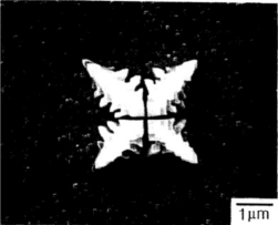
(a) Split dendrite [16].

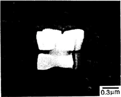
(b) Octodendritic structure [16].

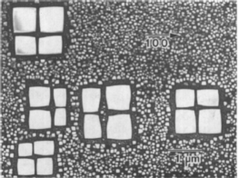
(c) Split pattern [15]

Figure 1: Experimental observations of split patterns (a) Formation of split dendritic structure when undercooled just below solvus temperature in model Ni-base superalloy [16]. (b) High magnification micrograph showing fissure planes which appeared to grow on the surface of $\gamma^{\prime}$ precipitate in model Ni-base superalloy [16]. (c) Transmission electron micrograph of Ni-Al alloy aged at $1100$$\mathrm{\SIUnitSymbolCelsius}$ for $1$h. Here, several larger cuboidal particles split into smaller octets of cuboids [15].

Doi et al. explained the formation of doublet as well as octet morphologies in Ni-based alloys based on the hollowing mechanism [13]. As per this mechanism, the matrix phase renucleates at the centre of the precipitate and grows along $\langle 001\rangle$ directions leading to disintegration of the precipitate. Using two-dimensional phase-field simulations, Wang et al. showed the formation of a split pattern via hollowing mechanism [29]. They described the eigen-strain field in the system as a function of local composition field. During the precipitate growth, the composition field in the precipitate becomes inhomogeneous due to higher strain energy contribution, and a further doublet pattern forms by renucleating the matrix phase at the centre of the precipitate. Following a similar approach, Li et al. showed the formation of a quartet pattern in two-dimensions [30]. However, in the work of Wang et al. and Li et al. , the chosen values of elastic misfit for which splitting occurs are physically unrealistic. Moreover, with the help of phase-field simulations, Li and Chen also showed the formation of doublets under the influence of applied strain fields in an elastically inhomogeneous system [31]. In another work, Liu et al. reported the formation of block of split particles in a single as well as multiparticle systems using two-dimensional phase-fieldsimulations [32]. Further, they extended their work to show split dendrite using two-dimensional phase-field simulations under the influence of anisotropic interfacial energy and isotropic elastic energy [33]. Liu and co-workers obtained the split pattern from the initial configuration where the precipitate is highly under-saturated. However, according to the classical nucleation theory, the critical nucleus size of the matrix phase that can nucleate for such under-saturations can be comparable to that of the precipitate. Moreover, the physical basis for considering undersaturation of precipitates under isothermal conditions cannot be explained.

Banerjee et al. suggested an alternative mechanism of formation of split patterns in Ni-base alloys via particle aggregation. They used a coherent phase-field model that incorporates the evolution of anti-phase domains of $\mathrm{L}1_{2}$ ordered $\upgamma^{\prime}$ particles in a disordered $\upgamma$ matrix phase [34]. When the anti-phase boundary energy is higher than interfacial energy, the interactions between the four different ordered domains in a disordered matrix can result in a quartet and octet pattern in two dimensions and three dimensions, respectively. High-resolution electron microscopy (HREM) studies of Ni-base alloys corroborate the particle aggregation mechanism where different translational domains can migrate to form split patterns [35, 36, 37]. Using HREM, the statistical analysis of the phase relationships between the neighboring pairs of $\upgamma^{\prime}$ particles show that 72% of the particle pairs are out-of-phase relationship, i.e., one translational domain of $\upgamma^{\prime}$ particle surrounded by another translational domain of $\upgamma^{\prime}$ particle [36, 37]. Since all the four variants of $\gamma^{\prime}$ have equal thermodynamic possibility to randomly nucleate in the $\gamma$ matrix, nearly three quarters of particle pairs surrounding a given particle will statistically have out-of-phase relationship. However, this evidence does not suggest that the particle can aggregate to form a quartet or octet of the precipitate while isothermal aging. On the other hand, in a Cu-Zn-Al alloy, the $\upgamma$ brass phase has a complex $\mathrm{D}8_{2}$structure, which nucleates in the $\mathrm{B}2$ ordered $\upbeta$-brass matrix phase and shows a quartet pattern of $\upgamma$-brass precipitates [22]. Unlike four variants describing the $\upgamma^{\prime}$ precipitates in Ni-base alloys, the $\upgamma$-brass precipitate phase is described by 36 translational variants [38]; it is unclear to explain comprehensively how different translational variants lead to the formation of split patterns in Cu-Zn-Al alloy. Hence, particle aggregation mechanism may not explain the split patterns observed in Cu-Zn-Al alloy where an ordered precipitate with lower symmetry nucleates in an ordered matrix phase.

Kaufman et al. proposed that the formation of split patterns in Ni-Al alloy occurs via interfacial instability over the precipitate faces [15]. When the interfacial instability initiates on one or six faces of the particle, instability spreads through the particle towards the centre of the particle and leads to the formation of a split pattern. Using two-dimensional phase-field simulations, Cha et al. show the formation of the quartet pattern via morphological instability in an elastically inhomogeneous system [39]. In addition, few theoretical studies reported the effect of applied fields and elastic incommensurity on the particle splitting. Leo et al. show that the presence of the deviatoric stresses can lead to the particle splitting in an elastically inhomogeneous alloy system [40]. In a discrete atom method study, Lee shows that elastically incommensurate system (i.e., elastically soft direction of the matrix aligns along elastically hard directions of the precipitate) can form quartet patterns. However, reports of elastically incommensurate elastic constants in an alloy system such as Ni-base alloys are not present.

Amongst the previously discussed mechanisms, we rule out matrix renucleation and particle aggregation as the mechanisms to explain the splitting behaviour. It is possible that the splitting instability may initiate at the concavities present on the faces of the cuboidal precipitates, as many experimental observations show the formation of concavities on the faces of cuboidal particles during growth which forms owing to the point effect of diffusion [12, 16, 13, 41]. A sharp interface based equilibrium shape study conforms to this possibility where the presence of a notch on the face of precipitate oriented along $[10]$ direction is a precursor for the splitting of precipitate to occur in an elastically inhomogeneous system [42]. We hypothesize that kinetically driven morphological instability, e.g., dendrite-like structure, in an elastically anisotropic cubic alloy system can probably lead to the development of concavities at the centre of precipitate faces which further can develop grooves along $\langle 100\rangle$ and $\langle 110\rangle$ crystallographic directions ($\langle 10\rangle$ directions in two-dimensions). These grooves continue to run toward the centre of of the precipitate resulting in primary dendrite fragmentation. We are motivated to draw this hypothesis based on the capillary-driven fragmentation of dendrite side-arms observed during the solidification of alloys [43, 44].

In this work, we present the phase-field simulations of particle splitting instability in an elastically homogeneous and anisotropic alloy system which mimics the superalloys. We identify factors influencing the initiation of splitting instability; in particular, the effects of lattice misfit, the strength of anisotropy in elastic energy, and interactions between particles on the initiation of splitting instability in a modelled alloy system. Section 2 presents the phase-field model followed by two-dimensional as well as three-dimensional simulation results and their discussion in section 3. We derive the conclusions in section 4.

2 Model

A phase-field model based on free energy functional, e.g., Kim-Kim-Suzuki (KKS) model, needs to impose continuity of diffusion potential across the interface to exhibit a quantitative nature. It is unlike phase-field models based on grand-potential functional wherein the grand potential energy naturally possesses quantitative character. Using the Legendre transform, one can show that the grand-potential formalism is equivalent to the KKS formalism [45, 46]. Here, we employ the KKS formalism [47, 48] to perform the simulations of coherently misfitting two-phase modelled alloy system. In addition, we follow the extended Cahn-Hilliard model proposed by Abinandanan and Haider [49] to incorporate the anisotropy in interfacial energy by taking into account fourth derivatives in the free energy functional.

Sections 2.1 and 2.2 discuss the energetics and governing equations describing the evolution of field variables of the system, respectively. Further, we present the numerical implementation of the governing equations in section 2.3.

2.1 Energetics

Eqn. (1) represents the total free energy of a system described in terms of order parameter field $\phi(\mathbf{r})$ and composition fields $c_{\upalpha}(\mathbf{r})$ and $c_{\upbeta}(\mathbf{r})$ of phases $\upalpha$ (matrix) and $\upbeta$ (precipitate) respectively.

$$\mathcal{F}\left(\phi(\mathbf{r}),\nabla\phi(\mathbf{r}),c_{\upalpha}(\mathbf{r}),c_{\upbeta}(\mathbf{r})\right) = N_{\textrm{v}}\int_{V}\Big{[}f^{*}_{\textrm{dw}}+f_{\textrm{grad}}^{*}+f^{*}_{\textrm{ch}}+f_{\textrm{el}}^{*}\Big{]}\mathrm{d}V,$$ (1)

$$= \int_{V}\Big{[}f_{\textrm{dw}}+f_{\textrm{grad}}+f_{\textrm{ch}}+f_{\textrm{el}}\Big{]}\mathrm{d}V,$$

where $f_{\textrm{dw}}$ represents the double-well potential energy density of the system, $f_{\textrm{grad}}$ is the gradient-energy density, $f_{\textrm{ch}}$ is the chemical free-energy density of the system, $f_{\textrm{el}}$ is the elastic free-energy density of the system, $N_{\textrm{v}}$ denotes the number of atoms per unit volume in the system, and $V$ represents the volume of the system. The double-well potential energy density $f_{\textrm{dw}}$ reads as

$$f_{\textrm{dw}}(\phi)=\eta_{w}\phi^{2}(1-\phi)^{2},$$ (2)

where $\eta_{w}$ is the height of potential barrier of the double well potential. Here, $\phi=1$ denotes the precipitate phase, whereas $\phi=0$ is the matrix phase. The gradient-energy density is discussed in A. We represent the bulk chemical free-energy density $f_{\textrm{ch}}$ of the system as the interpolation between the chemical free-energy densities of two phases:

$$f_{\textrm{ch}}(c_{\upalpha},c_{\upbeta})=h(\phi)f^{\upbeta}(c_{\upbeta})+\left(1-h(\phi)\right)f^{\upalpha}(c_{\upalpha}),$$ (3)

where $f^{\upalpha}(c_{\upalpha})$ and $f^{\upbeta}(c_{\upbeta})$ are chemical free-energy densities of the designated phases, and $h(\phi)$ is an interpolation function which should ensure that $h(0)=0$, $h(1)=1$, and $0<h(\phi)<1$ when $0<\phi<1$. We choose $h(\phi)=\phi^{3}(6\phi^{2}-15\phi+10)$ which guarantees the contribution of the interpolated quantity to the interface to be relatively less. The chemical free-energy densities of the two phases are approximated as parabolic functions:

$$f^{\upalpha}(c_{\upalpha})=f_{0}^{\upalpha}(c_{\upalpha}-c_{\upalpha}^{\textrm{e}})^{2}$$ (4)

$$f^{\upbeta}(c_{\upbeta})=f_{0}^{\upbeta}(c_{\upbeta}-c_{\upbeta}^{\textrm{e}})^{2},$$ (5)

where $\displaystyle f_{0}^{\upalpha,\upbeta}$ correspond to curvatures of the chemical free-energy densities of the designated phases, and $c_{\upalpha,\upbeta}^{\textrm{e}}$ denote equilibrium compositions of the designated phases. The bulk elastic free-energy density $f_{\textrm{el}}$ of the system is given as

$$f_{\textrm{el}}(\phi) = N_{\textrm{v}}C^{*}_{ijkl}(\mathbf{r})\epsilon_{ij}^{\textrm{el}}(\mathbf{r})\epsilon_{kl}^{\textrm{el}}(\mathbf{r}),$$ (6)

$$= C_{ijkl}(\mathbf{r})\epsilon_{ij}^{\textrm{el}}(\mathbf{r})\epsilon_{kl}^{\textrm{el}}(\mathbf{r}),$$ (7)

where $C_{ijkl}(\mathbf{r})$ represents the position dependent component of the elastic stiffness tensor, $\epsilon_{ij}^{\textrm{el}}(\mathbf{r})$ is the elastic strain field which is represented as $\displaystyle\epsilon_{ij}^{\textrm{el}}(\mathbf{r})=\bar{\epsilon}_{ij}+\delta\epsilon_{ij}(\mathbf{r})-\epsilon_{ij}^{0}(\mathbf{r})$. Here, $\bar{\epsilon}_{ij}$ is the homogeneous strain in the system, $\delta\epsilon_{ij}(\mathbf{r})$ is the heterogeneous strain field which has no macroscopic effects on the system, and $\epsilon_{ij}^{0}(\mathbf{r})$ is the eigen-strain field. The heterogeneous strain is the symmetric part of the displacement gradient, i.e., $\displaystyle\delta\epsilon_{ij}(\mathbf{r})=\frac{1}{2}\left[\frac{\partial u_{i}(\mathbf{r})}{\partial r_{j}}+\frac{\partial u_{j}(\mathbf{r})}{\partial r_{i}}\right]$, where $u_{i}(\mathbf{r})$ represents the displacement field. We assume a dilatational eigen-strain field in the system which writes as $\epsilon_{ij}^{0}(\mathbf{r})=\epsilon^{*}\delta_{ij}h(\phi)$, where $\epsilon^{*}$ is the magnitude of eigen-strain and $\delta_{ij}$ is the Kronecker delta function.

2.2 Evolution Equations

The local composition field $c(\mathbf{r})$ is represented as the interpolation of the phase compositions $c_{\upalpha}$ and $c_{\upbeta}$:

$$c(\mathbf{r})=h(\phi)c_{\upbeta}+\left(1-h(\phi)\right)c_{\upalpha}.$$ (8)

The diffusion equation governs the evolution of local composition field $c(\mathbf{r})$ [47]:

$$\frac{\partial c(\mathbf{r})}{\partial t}=M\nabla^{2}\widetilde{\mu}=D\left[\nabla^{2}c(\mathbf{r})+\boldsymbol{\nabla}\cdot\left(h^{\prime}\left(\phi(\mathbf{r})\right)\left(c_{\upalpha}-c_{\upbeta}\right)\boldsymbol{\nabla}\phi\left(\mathbf{r}\right)\right)\right],$$ (9)

where $D$ is the inter-diffusion coefficient. In order to decouple the gradient and bulk energy contributions, we impose a sharp interface boundary condition of the equality of diffusion potentials across the interface [47] which is

$$\frac{\partial f^{\upalpha}(c_{\upalpha})}{\partial c_{\upalpha}}=\frac{\partial f^{\upbeta}(c_{\upbeta})}{\partial c_{\upbeta}}.$$ (10)

The Allen-Cahn equation governs the evolution of order parameter field $\phi(\mathbf{r})$ [50]:

$$\frac{\partial\phi(\mathbf{r})}{\partial t}=-L\frac{\delta\mathcal{F}}{\delta\phi(\mathbf{r})}=L\left[2\varepsilon^{2}\nabla^{2}\phi-f^{\prime}_{\textrm{dw}}-f^{\prime}_{\textrm{ch}}-f^{\prime}_{\textrm{el}}\right],$$ (11)

where $L$ denotes the relaxation coefficient, primed quantities represent the derivatives with respect to $\phi$. The derivative of elastic driving force $f_{\mathrm{el}}^{\prime}$ is presented in B.

Since the elastic field relaxes faster than $\phi$ or $c$, it is reasonable to assume the stress field $\sigma(\mathbf{r})$ in the system to be governed by static equilibrium, given as

$$\nabla_{j}\sigma_{ij}(\mathbf{r})=0,$$ (12)

where $\sigma_{ij}(\mathbf{r})$ is the local stress field present in the system. We implement the Khachaturyan’s interpolation scheme [51] to describe the local stress field in the system:

$$\sigma_{ij}(\mathbf{r})=C_{ijkl}(\mathbf{r})\left(\bar{\epsilon}_{kl}+\delta\epsilon_{kl}(\mathbf{r})-\epsilon^{0}_{kl}(\mathbf{r})\right).$$ (13)

The position dependent stiffness tensor reads as

$$C_{ijkl}(\mathbf{r})=C_{ijkl}^{0}+C_{ijkl}^{\prime}(\mathbf{r}),$$ (14)

where $C_{ijkl}^{0}=\frac{1}{2}(C_{ijkl}^{\upbeta}+C_{ijkl}^{\upalpha})$ is the homogeneous elastic stiffness tensor and $C_{ijkl}^{\prime}(\mathbf{r})=\frac{1}{2}(C_{ijkl}^{\upbeta}-C_{ijkl}^{\upalpha})(2h(\phi)-1)$ is the heterogeneous elastic stiffness tensor. $C_{ijkl}^{\upbeta}$ and $C_{ijkl}^{\upalpha}$ are elastic stiffness tensors of the designated phases. Combining Eqns. (12), (13) and (14), and further simplifying, we can write the mechanical equilibrium equation as

$$C_{ijkl}^{0}\frac{\partial^{2}u_{k}}{\partial r_{j}\partial r_{l}}=\nabla_{j}\left[C_{ijkl}(\mathbf{r})\left(\epsilon_{kl}^{0}(\mathbf{r})-\bar{\epsilon}_{kl}\right)+C_{ijkl}^{\prime}(\mathbf{r})\frac{\partial u_{k}}{\partial r_{l}}.\right]$$ (15)

Eqn. (15) represents one of the conditions of mechanical equilibrium given by Khachaturyan’s micro-elasticity theory. One needs to impose the another necessary condition of mechanical equilibrium, i.e., [51]

$$\frac{\partial f_{\textrm{el}}}{\partial\bar{\epsilon}_{ij}}=0.$$ (16)

Further simplifying Eqn. (16), we get

$$\bar{\epsilon}_{ij}=\langle S_{ijkl}\rangle\left(\langle\sigma^{0}_{kl}\rangle-\langle\delta\sigma_{kl}\rangle\right),$$ (17)

where $\langle S_{ijkl}\rangle=\langle C_{ijkl}\rangle^{-1}$, $\langle C_{ijkl}\rangle=1/V\int_{V}C_{ijkl}(\mathbf{r})\mathrm{d}V$,
$\langle\sigma_{ij}^{0}\rangle=1/V\int_{V}C_{ijkl}(\mathbf{r})\epsilon^{0}_{kl}(\mathbf{r})\mathrm{d}V$, $\langle\delta\sigma_{ij}\rangle=1/V\int_{V}C_{ijkl}(\mathbf{r})\delta\epsilon_{kl}(\mathbf{r})\mathrm{d}V$. Eqns. (15) and (17) constitute the set of governing equations which ensure that the mechanical equilibrium is attained in the system.

2.3 Numerical Implementation

We implement semi-implicit Fourier spectral method to obtain the solution to Eqns. (9) and (11) at every time step [52]. We seek the numerical solution of the displacement fields by spectral iterative perturbation method [53, 54]. Here, we show the discretized form of equations which are evolved at each time step to get solutions of $c(\mathbf{r},t)$ and $\phi(\mathbf{r},t)$ in Fourier space. Quantities with tilde represent the Fourier transform of corresponding quantities. The evolution of the local composition field in Fourier space reads as

$$\widetilde{c}(\boldsymbol{\xi},t+\Delta t)=\frac{\widetilde{c}(\boldsymbol{\xi},t)-ID\Delta t\;\boldsymbol{\xi}\cdot\widetilde{\mathbf{p}}(\boldsymbol{\xi},t)}{1+D\xi^{2}\Delta t},$$ (18)

where $I=\sqrt{-1}$, $\Delta t$ is the time increment, $\boldsymbol{\xi}$ denotes the inverse space vector, $\xi$ is the magnitude of $\boldsymbol{\xi}$, $\widetilde{\mathbf{p}}(\boldsymbol{\xi},t)$ represents the Fourier transform of $\mathbf{p}(\mathbf{r},t)=h^{\prime}(\phi)(c_{\upalpha}-c_{\upbeta})\boldsymbol{\nabla}\phi$. The evolution of the order parameter $\phi$ in Fourier space reads as

$$\widetilde{\phi}(\boldsymbol{\xi},t+\Delta t)=\frac{\widetilde{\phi}(\boldsymbol{\xi},t)-L\widetilde{m}(\boldsymbol{\xi},t)\Delta t}{1+2\varepsilon^{2}\xi^{2}\Delta t},$$ (19)

where $\widetilde{m}(\boldsymbol{\xi},t)$ represents the Fourier transform of $\displaystyle m(\mathbf{r},t)=f^{\prime}_{\textrm{dw}}+f^{\prime}_{\textrm{ch}}+f^{\prime}_{\textrm{el}}$.

The spectral iterative perturbation method involves the evaluation of displacement fields for a homogeneous system, i.e., zeroth-order approximation, and further higher-order approximations are obtained up to the prescribed tolerance level by substituting the previous order approximations. Eqns. (20) and (21) represent respectively the zeroth and higher-order approximations of the displacement fields in Fourier space.

$$\widetilde{u}^{(0)}_{k}(\boldsymbol{\xi})=-I\xi_{j}G_{ik}(\boldsymbol{\hat{\xi}})\widetilde{\sigma}^{0}_{ij}(\boldsymbol{\xi}),$$ (20)

$$\widetilde{u}_{k}^{(\textrm{n})}(\boldsymbol{\xi})=-I\xi_{j}G_{ik}(\boldsymbol{\hat{\xi}})\left[C_{ijpq}(\mathbf{r})\left(\epsilon_{pq}^{0}(\mathbf{r})-\bar{\epsilon}_{pq}\right)+C_{ijpq}^{\prime}(\mathbf{r})\frac{\partial u_{p}^{(\mathrm{n}-1)}(\mathbf{r})}{\partial r_{q}}\right]_{\boldsymbol{\xi}},$$ (21)

where $G_{ik}$ represents the Green tensor whose inverse is given as $(G_{ik})^{-1}=C_{ijkl}^{0}\hat{\xi}_{j}\hat{\xi}_{l}$, $\displaystyle\boldsymbol{\hat{\xi}}=\frac{\boldsymbol{\xi}}{|\boldsymbol{\xi}|}$, $\xi_{j}$ denotes the components of inverse space vector, $\widetilde{\sigma}_{ij}^{0}(\boldsymbol{\xi})$ is the Fourier transform of $\sigma_{ij}^{0}(\mathbf{r})$, $[\cdot]_{\boldsymbol{\xi}}$ represents the quantity in Fourier space. Previous phase-field studies [39] evaluate displacement field only up to the third order that can result in appreciable error in the stress field of the system. Since we impose homogeneous moduli approximation in the system, Eqn. (20) is sufficient to seek solution for the displacement field.

2.4 Sharp-interface limit

In this section, we show that in the sharp-interface limit, we recover the Gibbs-Thomson relation from our diffuse-interface model when the interface is curved and coherent. Here, we assume a coordinate system where normal ($\mathbf{n}$) and tangent vector ($\mathbf{t}$) to the interface constitute the basis vectors. The normal to the interface is given as

$$\boldsymbol{\nabla}\phi=\mathbf{n}\frac{\partial\phi}{\partial n}.$$ (22)

Upon taking divergence of (22),

$$\nabla^{2}\phi=\frac{\partial^{2}\phi}{\partial n^{2}}+\frac{\partial\phi}{\partial n}\left(\boldsymbol{\nabla}\cdot\mathbf{n}\right).$$ (23)

The phase-field equation in the transformed coordinate is

$$\frac{1}{L}\frac{\partial\phi(\mathbf{r})}{\partial t}= 2\varepsilon^{2}\left(\frac{\partial^{2}\phi}{\partial n^{2}}+\frac{\partial\phi}{\partial n}\left(\nabla\cdot\mathbf{n}\right)\right)-2\eta_{\mathrm{w}}\phi(1-2\phi)(1-\phi)$$

$$-h^{\prime}(\phi)\left[f^{\upbeta}(c_{\upbeta})-f^{\upalpha}(c_{\upalpha})-(c_{\upbeta}-c_{\upalpha})\frac{\partial f^{\upalpha}(c_{\upalpha})}{\partial c_{\upalpha}}\right]-f_{\textrm{el}}^{\prime}.$$ (24)

The leading order solution for the phase-field profile $\phi_{0}$ is:

$$2\varepsilon^{2}\frac{\partial^{2}\phi_{0}}{\partial n^{2}}-2\eta_{\mathrm{w}}\phi_{0}(1-2\phi_{0})(1-\phi_{0})=0.$$ (25)

After multiplying $\displaystyle\frac{\partial\phi_{0}}{\partial n}$ on both sides of Eqn. (25) and integrating it along the interface normal at the boundary such that in the bulk of matrix and precipitate $\displaystyle\frac{\partial\phi_{0}}{\partial n}=0$,

$$\varepsilon^{2}\left(\frac{\partial\phi_{0}}{\partial n}\right)^{2}=\eta_{\mathrm{w}}\phi_{0}^{2}(1-\phi_{0})^{2}$$ (26)

Solving Eqn. (26) gives a equilibrium phase-field profile without any driving force. After combining Eqns. (24) and (25), the updated phase-field equation is

$$\frac{1}{L}\frac{\partial\phi}{\partial t}= 2\varepsilon^{2}\left(\frac{\partial\phi_{0}}{\partial n}(\nabla\cdot\mathbf{n})\right)-h^{\prime}(\phi)\left[f^{\upbeta}(c_{\upbeta})-f^{\upalpha}(c_{\upalpha})-(c_{\upbeta}-c_{\upalpha})\frac{\partial f^{\upalpha}(c_{\upalpha})}{\partial c_{\upalpha}}\right]$$

$$-f_{\textrm{el}}^{\prime}$$ (27)

In a sharp-interface limit, we can obtain the elastic driving force $f_{\textrm{el}}^{\prime}=\frac{\partial f_{\textrm{el}}}{\partial\phi}$:

$$\frac{\partial f_{\textrm{el}}}{\partial\phi}=\frac{\mathrm{d}f_{\textrm{el}}}{\mathrm{d}\phi}-\frac{\partial f_{\textrm{el}}}{\partial\epsilon_{nn}}\frac{\partial\epsilon_{nn}}{\partial\phi}-2\frac{\partial f_{\textrm{el}}}{\partial\epsilon_{nt}}\frac{\partial\epsilon_{nt}}{\partial\phi}-\frac{\partial f_{\textrm{el}}}{\partial\epsilon_{tt}}\frac{\partial\epsilon_{tt}}{\partial\phi}$$ (28)

At the sharp-interface limit, $\sigma_{tt}$ exhibits a jump and $\sigma_{nn}$ and $\sigma_{nt}$ will be continuous across the interface, i.e., $\sigma_{nn}^{\upalpha}=\sigma_{nn}^{\upbeta}=\sigma_{nn}^{0}$ and $\sigma_{nt}^{\upalpha}=\sigma_{nt}^{\upbeta}=\sigma_{nt}^{0}$. Hence, $\sigma_{tt}$ vanishes in the sharp-interface limit. As a result, the leading order elastic driving force in the sharp-interface limit is expressed as

$$\frac{\partial f_{\textrm{el}}}{\partial\phi}=\frac{\mathrm{d}f_{\textrm{el}}}{\mathrm{d}\phi}-\sigma_{nn}^{0}\frac{\partial\epsilon_{nn}}{\partial\phi}-2\sigma_{nt}^{0}\frac{\partial\epsilon_{nt}}{\partial\phi}=\frac{\mathrm{d}}{\mathrm{d}\phi}\left[f_{\textrm{el}}-\sigma_{nn}^{0}\epsilon_{nn}-2\sigma_{nt}^{0}\epsilon_{nt}\right]$$ (29)

Inserting Eqn. (29) in Eqn. (27),

$$\frac{1}{L}\frac{\partial\phi}{\partial t}= 2\varepsilon^{2}\left(\frac{\partial\phi_{0}}{\partial n}(\nabla\cdot\mathbf{n})\right)-h^{\prime}(\phi)\left[f^{\upbeta}(c_{\upbeta})-f^{\upalpha}(c_{\upalpha})-(c_{\upbeta}-c_{\upalpha})\frac{\partial f^{\upalpha}(c_{\upalpha})}{\partial c_{\upalpha}}\right]$$

$$-\frac{\mathrm{d}}{\mathrm{d}\phi}\left[f_{\textrm{el}}-\sigma_{nn}^{0}\epsilon_{nn}-2\sigma_{nt}^{0}\epsilon_{nt}\right].$$ (30)

Multiplying both sides of Eqn. (30) by $\displaystyle\frac{\partial\phi_{0}}{\partial n}$ and integrating from the bulk of the precipitate to that of the matrix along normal to the interface, we derive

$$\frac{1}{L}\int_{\textrm{in}}^{\textrm{out}}\frac{\partial\phi}{\partial t}\frac{\partial\phi_{0}}{\partial n}\mathrm{d}n= 2\varepsilon^{2}\int_{\textrm{in}}^{\textrm{out}}\left(\frac{\partial\phi_{0}}{\partial n}\right)^{2}(\nabla\cdot\mathbf{n})\mathrm{d}n$$

$$-\int_{1}^{0}h^{\prime}(\phi)\left[f^{\upbeta}(c_{\upbeta})-f^{\upalpha}(c_{\upalpha})-(c_{\upbeta}-c_{\upalpha})\frac{\partial f^{\upalpha}(c_{\upalpha})}{\partial c_{\upalpha}}\right]\mathrm{d}\phi$$

$$-\int_{1}^{0}\frac{\mathrm{d}}{\mathrm{d}\phi}\left[f_{\textrm{el}}-\sigma_{nn}^{0}\epsilon_{nn}-2\sigma_{nt}^{0}\epsilon_{nt}\right]\mathrm{d}\phi$$ (31)

The left-hand term in Eqn. (31) can be simplified as

$$\frac{\partial\phi}{\partial t}\frac{\partial\phi_{0}}{\partial n}=-\left(\frac{\partial n}{\partial t}\right)_{\phi}\left(\frac{\partial\phi_{0}}{\partial n}\right)^{2}=-V_{\textrm{n}}\left(\frac{\partial\phi_{0}}{\partial n}\right)^{2},$$ (32)

where $V_{n}$ denotes the velocity of the interface. $\nabla\cdot\mathbf{n}=-\kappa$ denotes the mean curvature of the interface. Hence, Eqn. (31) is modified as

$$-\frac{V_{\textrm{n}}}{L}\int_{\textrm{in}}^{\textrm{out}}\left(\frac{\partial\phi_{0}}{\partial n}\right)^{2}\mathrm{d}n= -2\varepsilon^{2}\kappa\int_{\textrm{in}}^{\textrm{out}}\left(\frac{\partial\phi_{0}}{\partial n}\right)^{2}\mathrm{d}n$$

$$-\left[f^{\upbeta}(c_{\upbeta})-f^{\upalpha}(c_{\upalpha})-(c_{\upbeta}-c_{\upalpha})\frac{\partial f^{\upalpha}(c_{\upalpha})}{\partial c_{\upalpha}}\right]\Bigg{.}h(\phi)\Bigg{|}_{1}^{0}$$

$$-\left[f_{\textrm{el}}-\sigma_{nn}^{0}\epsilon_{nn}-2\sigma_{nt}^{0}\epsilon_{nt}\right]_{1}^{0}$$ (33)

The term $\displaystyle\int_{\textrm{in}}^{\textrm{out}}\left(\frac{\partial\phi_{0}}{\partial n}\right)^{2}\mathrm{d}n$ corresponds to $\displaystyle\frac{\gamma}{2\varepsilon^{2}}$. After invoking the equality of diffusion potentials, i.e., $\displaystyle\frac{\partial f^{\upalpha}(c_{\upalpha})}{\partial c_{\upalpha}}=\frac{\partial f^{\upbeta}(c_{\upbeta})}{\partial c_{\upbeta}}$, we rewrite the Eqn. (33) as

$$V_{\textrm{n}}=M^{\textrm{eff}}\left[\gamma\kappa+(\Psi^{\upalpha}-\Psi^{\upbeta})+(\omega^{\upalpha}-\omega^{\upbeta})\right],$$ (34)

where

$$M^{\textrm{eff}} = \frac{2\varepsilon^{2}L}{\gamma},$$ (35)

$$\Psi^{\upalpha} = f^{\upalpha}(c_{\upalpha})-c_{\upalpha}\frac{\partial f^{\upalpha}(c_{\upalpha})}{\partial c_{\upalpha}},$$ (36)

$$\Psi^{\upbeta} = f^{\upbeta}(c_{\upbeta})-c_{\upbeta}\frac{\partial f^{\upbeta}(c_{\upbeta})}{\partial c_{\upbeta}},$$ (37)

$$\omega^{\upalpha} = f_{\textrm{el}}^{\upalpha}-\sigma_{nn}^{0}\epsilon_{nn}^{\upalpha}-2\sigma_{nt}^{0}\epsilon_{nt}^{\upalpha},$$ (38)

$$\omega^{\upbeta} = f_{\textrm{el}}^{\upbeta}-\sigma_{nn}^{0}\epsilon_{nn}^{\upbeta}-2\sigma_{nt}^{0}\epsilon_{nt}^{\upbeta},$$ (39)

and $\Psi^{\upalpha,\upbeta}$ represents the grand potential densities of the designated phases. We are interested in diffusion-controlled growth regime, therefore phase-field $\phi$ relaxes infinitely fast, i.e., $M^{\textrm{eff}}=\infty$, and as a result

$$\gamma\kappa+(\Psi^{\upalpha}-\Psi^{\upbeta})+(\omega^{\upalpha}-\omega^{\upbeta})=0$$ (40)

The driving force for phase transformation $\Delta\Psi=\Psi^{\upbeta}-\Psi^{\upalpha}$ balances the curvature and the elastic driving forces

$$\Delta\Psi=\Psi^{\upbeta}-\Psi^{\upalpha}=\gamma\kappa+(\omega^{\upalpha}-\omega^{\upbeta}).$$ (41)

Using the linear expansion of grand potential about the chemical potential [45, 46]

$$\Delta\Psi=\left(\frac{\partial\Psi^{\upbeta}}{\partial\mu}-\frac{\partial\Psi^{\upalpha}}{\partial\mu}\right)\Delta\mu,$$ (42)

where $\Delta\mu=\mu-\mu_{\textrm{eq}}$, and $\mu_{\textrm{eq}}$ represents the equilibrium chemical potential. After invoking thermodynamic relation $\displaystyle\frac{\partial\Psi}{\partial\mu}=-c$,

$$(c_{\upalpha}-c_{\upbeta})\Delta\mu=\gamma\kappa+(\omega^{\upalpha}-\omega^{\upbeta}).$$ (43)

Performing linear expansion of chemical potential about the composition of $\upbeta$ phase, we derive

$$(c_{\upalpha}-c_{\upbeta})\frac{\partial\mu}{\partial c}(c_{\upbeta}-c_{\upbeta}^{\textrm{e}})=(c_{\upalpha}-c_{\upbeta})\frac{\partial^{2}f^{\upbeta}}{\partial c^{2}_{\upbeta}}(c_{\upbeta}-c_{\upbeta}^{e})=\gamma\kappa+(\omega^{\upalpha}-\omega^{\upbeta}).$$ (44)

Thus, we obtain a Gibbs-Thomson relation for the shift in the equilibrium composition of $\upbeta$ phase

$$\Delta c_{\mathrm{\upbeta}}=\frac{\gamma\kappa+(\omega^{\upalpha}-\omega^{\upbeta})}{\frac{\partial^{2}f^{\upbeta}}{\partial c^{2}_{\upbeta}}(c_{\upalpha}-c_{\upbeta})}.$$ (45)

Eqn. 45 provides the interfacial compositions for $\upalpha$ and $\upbeta$ phases. Further, the mass balance equation extends the normal velocity of the interface under the diffusion controlled regime, i.e.,

$$V_{\mathrm{n}}(c_{\upbeta}^{\prime}-c_{\upalpha}^{\prime})=D(\boldsymbol{\nabla}c_{\upbeta}^{\prime}-\boldsymbol{\nabla}c_{\upalpha}^{\prime})\cdot\mathbf{n},$$ (46)

Here $\displaystyle c_{\upbeta,\upalpha}^{\prime}=c_{\upbeta,\upalpha}^{e}+\Delta c_{\upbeta,\upalpha}$ represent the bulk compositions of $\upbeta$ and $\upalpha$ phases where the curvature and elastic contributions are accounted.

We compare the interfacial compositions from the simulations with that of the sharp-interface model in the asymptotic limits. We assume a circular precipitate ($\upbeta$) growing in a supersaturated matrix phase ($\upalpha$). Fig. 2 shows that the asymptotic extensions of the bulk values of $\sigma_{nn}^{\upalpha},\sigma_{nn}^{\upbeta}$ and $\epsilon_{tt}^{\upalpha},\epsilon_{tt}^{\upbeta},\epsilon_{nt}^{\upalpha},\epsilon_{nt}^{\upbeta}$ to the interface from diffuse interface simulation clearly captures the continuity of normal stresses and transverse strain fields. Other stress and strain fields exhibit jump across the interface. Fig.3 shows the comparison of the interfacial compositions from sharp-interface model and diffuse interface. The shift in composition from the sharp-interface model comes out to be $0.0417$ and the corresponding shift in composition from the diffused interface simulations is $0.0506$. The interfacial conditions in the simulations compare well with sharp-interface model in the asymptotic limits.

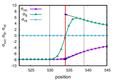
(a)

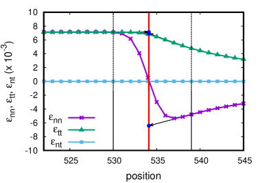
(b)

Figure 2: (a) Stress and (b) strain profiles across the interface of the cylindrical precipitate growing in a supersaturated matrix. The solid red line indicates the position of interface at $\phi=0.5$. The asymptotic extensions of the normal stress and transverse strain are continuous at the interface. On the other hand, transverse stress and normal strain fields exhibit jump across the interface.

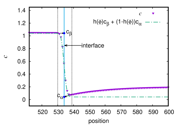
Figure 3: Composition profile of the circular precipitate in a supersaturated matrix ($c_{\infty}=20\%$). Here, we assume isotropic homogeneous moduli approximation with lattice misfit of $1\%$ and shear modulus of $550$.

3 Results

We have performed two-dimensional as well as three-dimensional phase-field simulations of single and two precipitates in a supersaturated matrix. The morphological evolution is characterized by the quantification of Gibbs-Thomson effect. We investigate the effect of lattice misfit, anisotropy in elastic energy, and particle interactions on the morphological evolution.

3.1 Generalized Gibbs-Thomson effect

During the growth of coherently misfitting precipitate, the curvature and elastic effects shift the equilibrium composition of the matrix which in turn shifts the chemical potential present in the matrix, i.e., Gibbs-Thomson effect [55, 56]. Depending on the strengths of lattice misfit and anisotropy in elastic energy, the contribution of elastic effects varies in different directions. We evaluate the shift in chemical potential ($\Delta\mu^{*}$) in the matrix phase ahead of interface as a function of an arc-length ($l_{\mathrm{arc}}$). The shift in chemical potential have two contributions, viz., curvature ($\Delta\mu^{\textrm{K}*}$) and elastic effects ($\Delta\mu^{\mathrm{el}*}$):

$$\Delta\mu^{*}=\Delta\mu^{\textrm{K}*}+\Delta\mu^{\textrm{el}*},$$ (47)

where $\displaystyle\Delta\mu^{\textrm{K}*}=\frac{\gamma\kappa}{(c_{\upbeta}^{\textrm{e}}-c_{\upalpha}^{\textrm{e}})}$, $\kappa$ is the mean curvature and $\gamma$ is the interfacial energy. In a non-dimensional form, Eqn. (47) is rewritten as

$$\Delta\mu=l_{0}\kappa+\Delta\mu^{\textrm{el}},$$ (48)

where $\displaystyle\Delta\mu=\frac{l_{0}\Delta\mu^{*}}{\gamma}$, $\displaystyle\Delta\mu^{\textrm{el}}=\frac{l_{0}\Delta\mu^{\textrm{el}*}}{\gamma}$, $l_{0}$ is the characteristic length which we choose as $1\text{\,}\mathrm{nm}$.

%subsectionTopological characterization

3.2 Simulations Parameters

The thermodynamic and mobility parameters chosen in our study correspond to those of Ni-$17$ at.% Al alloy aged at $1000\text{\,}\mathrm{\SIUnitSymbolCelsius}$ where Kaufman et al. [15] reported the formation of split patterns of $\gamma^{\prime}$. Table 1 lists these parameters in dimensional as well as non-dimensional values. We use characteristic energy $\mathcal{E}=10^{-20}$ $\mathrm{J}$, characteristic length $\mathcal{L}=0.25$ $\mathrm{nm}$, and characteristic time $\mathcal{T}=3\times 10^{-3}$ $\mathrm{s}$.

Table 1: Simulation parameters used in simulations. Both dimensional and non-dimensional values of parameters are given.

Parameter	Non-dimensional value	Dimensional value	Formula
Interfacial energy ($\gamma$)	$0.12$	$20$ $\mathrm{mJ}\text{\,}{\mathrm{m}}^{-2}$	$\gamma=\gamma^{*}(\mathcal{E}\mathcal{L}^{-2})$
Interface width ($2\lambda$)	$1.6$	$0.4$ $\mathrm{nm}$	$2\lambda=(2\lambda)^{*}\mathcal{L}$
Inter-diffusion coefficient ($D$)	$1.0$	$10^{-15}$ ${\mathrm{m}}^{2}\text{\,}{\mathrm{s}}^{-1}$	$D=D^{*}\mathcal{L}^{2}\mathcal{T}^{-1}$
Relaxation coefficient ($L$)	$1.615$	$3.5\times 10^{-5}$ ${\mathrm{m}}^{2}\text{\,}{\mathrm{N}}^{-1}\text{\,}{\mathrm{s}}^{-1}$	$L=L^{*}\mathcal{L}^{3}\mathcal{E}^{-1}\mathcal{T}^{-1}$
Time step ($dt$)	$0.1$	$0.3$ $\mathrm{ms}$	$dt=dt^{*}\mathcal{T}$
Shear modulus ($G$)	$550$	$88$ $\mathrm{GPa}$	$G=G^{*}\mathcal{E}\mathcal{L}^{-3}$
Poisson’s ratio ($\nu$)	–	$0.3$	–
Zener anisotropy parameter ($A_{\textrm{z}}$)	–	$4-2$	–
Elastic misfit ($\epsilon^{*}$)	–	$0.5-1\%$	–
supersaturation ($c_{\infty}$)	–	$25-45\%$	–

By choosing $2\lambda=$ $0.4\text{\,}\mathrm{nm}$ and $dx=dy=dz=$ $0.05\text{\,}\mathrm{nm}$, we have ensured a minimum of eight grid points at the interface of $\phi$. The inter-diffusion coefficient $D=10^{-15}$ ${\mathrm{m}}^{2}\text{\,}{\mathrm{s}}^{-1}$ [57] and relaxation coefficient $L=3.5\times 10^{-5}$ ${\mathrm{m}}^{2}\text{\,}{\mathrm{N}}^{-1}\text{\,}{\mathrm{s}}^{-1}$ assure the diffusion-controlled growth of precipitate in a supersaturated matrix. We employ relations given by Schmidt and Gross [58] to represent the components of the stiffness tensor in Voigt’s notation for a system with cubic anisotropy in terms of average shear modulus ($G$), Poisson’s ratio ($\nu$), and Zener anisotropy parameter ($A_{\textrm{z}}$).

$$C_{11} =G\left[\frac{2(2+A_{\textrm{z}})}{1+A_{\textrm{z}}}-\frac{1-4\nu}{1-2\nu}\right];$$

$$C_{12} =G\left[\frac{2A_{\textrm{z}}}{1+A_{\textrm{z}}}-\frac{1-4\nu}{1+A_{\textrm{z}}}\right];$$

$$C_{44} =G\left[\frac{2A_{\textrm{z}}}{1+A_{\textrm{z}}}\right]$$

Following sections discuss the effects of elastic misfit, anisotropy in elastic energy, and degree of supersaturation on the particle splitting instability in three-dimensions. Since the three-dimensional simulations are memory intensive, we discuss the effect of particle interactions in two-particle settings using two-dimensional simulations. We perform both two-dimensional as well as three-dimensional simulations using NVIDIA Tesla V100 GPUs and utilize CUDA fast Fourier transform (cuFFT) library [59] to evaluate discrete Fourier transforms required for evolving Eqns. (18), (19), (20), and (21). The simulation parameters, hereafter, render non-dimensional values.

3.3 Evolution of precipitate morphology to split patterns

We begin with an isolated precipitate of size $3$ in a supersaturated matrix at the centre of the simulation box. Here, we choose supersaturation of $45\%$, lattice misfit of $0.85\%$, and Zener anisotropy parameter of $4$. Table 2 shows the evolution of precipitate morphology in isosurface view, and composition and order parameter map in $(110)$ plane passing through the centre of the simulation box at different simulation times. Initially, the spherical precipitate transforms to a cuboidal shape and ears start developing along $\langle 111\rangle$ directions. Later, the dendrite-like instability develops which exhibits predominant primary arms along $\langle 111\rangle$ directions (see precipitate morphology at $t=100$ in table 2). The formation of dendrite-like morphologies can be explained based on theory of morphological instability in coherent system given by Leo-Sekerka [26]. The morphological instability occurs when the point effect of diffusion dominates over the capillary forces. Further, during the growth of dendrite-like instability, the concavities are developed along faces directed towards $\langle 100\rangle$ and $\langle 110\rangle$ directions. These concavities develop grooves that advance towards the centre of precipitate from the faces and lead to the split morphology consisting of eight smaller precipitates (ogdoad) (see precipitate morphologies at $t=1000$, $5000$, and $10000$ in table 2).

	$t=100$	$t=1000$	$t=5000$	$t=10000$
Isosurface view
Composition map
Order Parameter map

Table 2: Temporal evolution of the precipitate morphology at time $t=100,\,1000,\,5000,\,10000$ $\mathrm{s}$. First row shows the isosurface representation of precipitate morphology. Second row shows the composition map in $(110)$ plane passing through the centre of the simulation box, and third row shows the corresponding order parameter map.

By following the evolution of precipitate morphology with a finer time-steps, we observe that the primary arms of dendrite-like structure pinch off from the precipitate core. Fig. 4 shows the evolution of precipitate morphology in the $(110)$ plane where primary arms pinch off from the precipitate core (see Fig. 4(b)). Further, the remaining precipitate core at the centre of the box dissolves completely. The separation of primary arms from the precipitate core is similar to secondary arms separating from the primary arms during dendritic growth in solidification. The pinch-off of secondary arms from the primary arms during solidification is a curvature driven process, whereas the pinch-off of primary arms during solid-state transformation is an elastically induced instability.

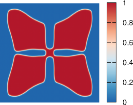
(a) $t=1100$

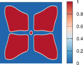
(b) $t=1200$

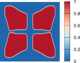
(c) $t=1300$

Figure 4: Evolution of precipitate morphology to split pattern in $(110)$ plane. (a) The precipitate morphology just before pinch off at $t=1100$. (b) The primary arms pinch off from the central precipitate core at time $t=1200$. (c) The remaining central precipitate core dissolves and a split pattern is formed. Here, $t=1300$.

Moreover, we plot composition fluxes to understand the flow of composition before the pinch-off of primary arms. Fig. 5(a) depicts the compositional fluxes at time $t=500$. The composition flow is predominantly towards the precipitate suggesting growth of precipitate. On the other hand, Fig. 5(b) shows the compositional fluxes at time $t=1000$ where composition flows outward from the precipitate in the groove regions (red colored flux lines) and solute deposits at the faces and tip of primary arms of the precipitate (green colored flux lines). The preferential dissolution in the grooves will be explained later in this section.

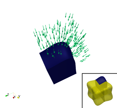
(a) $t=50$

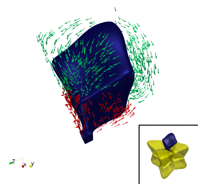
(b) $t=1000$

Figure 5: Compositional flux lines for time (a) $t=50$ (b) $t=1000$. At $t=50$, compositional flux lines are directed towards the particle which suggests growth of precipitate. At $t=1000$, some of the flux lines (red colored) are directed away from the precipitate surface which leads to dissolution, whereas green colored flux lines exhibit composition flow towards the precipitate.

Previous reports show that particle splitting occurs under the influence of interfacial energy anisotropy and isotropic elastic energy [33]. We investigate the effect of anisotropy in interfacial energy on the initiation of splitting of particle where the lattice misfit is ignored. To understand whether the anisotropy in interfacial energy can promote the splitting instability, we have performed two-dimensional simulations under the effect of anisotropy in interfacial energy. Fig. 6 represents the temporal evolution of the precipitate morphology in two-dimensions where we choose interfacial energy along $\langle 11\rangle$ directions ($\gamma_{11}$) one and twenty-five hundredth of that along $\langle 10\rangle$ directions ($\gamma_{10}$), where $\gamma_{10}$ is $0.122223$. The simulation box size is $1024\times 1024$ with the grid size of $0.5$. Here, we neglect the effect of elastic stresses on the growth of precipitate. In the presence of interfacial energy anisotropy, the initial circular precipitate develop ears, and subsequently prominent primary arms develop along $\langle 11\rangle$ directions. Although the precipitate faces develop concavities, the grooves never advance towards the centre of the precipitate. Thus, this result implies that the presence of elastic stresses and the anisotropy in elastic energy is necessary for splitting to occur. However, different combinations of interfacial energy anisotropy and elastic energy anisotropy can either promote or suppress the splitting of precipitate. Here after, we only present the simulations where the interfacial energy is isotropic.

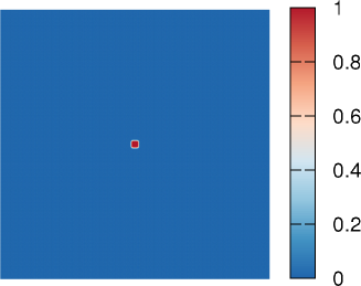
(a) $t=100$

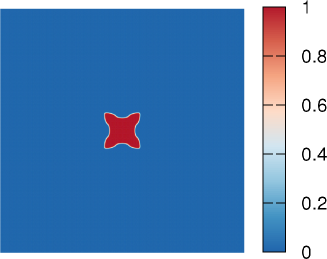
(b) $t=2000$

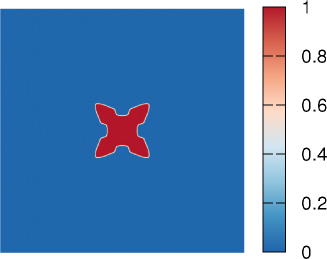
(c) $t=3000$

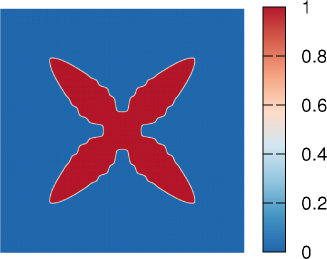
(d) $t=10000$

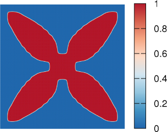
(e) $t=30000$

Figure 6: Temporal snapshots of precipitate morphology at time $t=100$, $2000$, $3000$, $10000$, and $30000$. Here, the elastic stresses are neglected and interfacial energy along $\langle 11\rangle$ direction is $1.25$ times of that along $\langle 10\rangle$ direction.

Similar to three-dimensional simulations, we have performed two-dimensional simulations of the precipitate growth in the simulation box size of $809.6\times 809.6$. We choose supersaturation of $25\%$, elastic misfit of $0.85\%$, and Zener anisotropy parameter of $4$. Table 3 depicts the temporal evolution of precipitate morphology in two-dimensions at different time steps.The initial circular precipitate transforms to square shape and gradually ears start developing along $[11]$ directions (see Fig. 3). At subsequent stages, predominant primary arms develop along $[11]$ directions, and simultaneously concavities start building up along $[10]$ directions. Unlike three-dimensional simulation morphology, here the prominent secondary arms are observed. Further, the grooves developed along $[10]$ directions advance towards the centre of the precipitate and subsequent pinch-off takes place. Later, the secondary arms start disappearing and facets of the split particles emerge to gradually orient towards $[10]$ directions.

$t=20000$	$t=40000$	$t=70000$	$t=300000$

Table 3: Temporal snapshots of precipitate morphology in two dimensions at $t=2000$, $20000$, $40000$, $70000$, $300000$. Here, supersaturation is $25\%$, misfit is $1\%$, and Zener anisotropy parameter is $4$.

The formation of a split pattern can be attributed to the higher contribution of elastic stresses to the shift in chemical potential ($\Delta\mu$) in directions where the grooves develop. To show that, we analyse the shift in chemical potential ahead of the interface in the matrix. Fig. 7(a) shows the order parameter map in $(110)$ plane at time $t=1100$, and the corresponding $\Delta\mu^{*}$ map is shown in Fig. 7(b). Fig. 7(c) shows the contour map at $\phi=0.5$ in the one-fourth section of $(110)$ plane passing through the centre of the simulation box. We track the $\Delta\mu$ ahead of the interface in the matrix phase along the contour line shown in Fig. 7(c) and plot the variation of $\Delta\mu$ in matrix along the contour as a function of arc-length $l_{\mathrm{arc}}$ as shown in Fig. 7(d). We obtain the arc-length by calculating the distance between the consecutive points on the contour in an anti-clockwise direction. The X-axis in the contour profile corresponds to $[\bar{1}10]$ direction, whereas the Y-axis corresponds to $[001]$. The tip of dendrite (directed along $[\bar{1}11]$) subtends an angle of $35.26$\mathrm{\SIUnitSymbolDegree}$$ with X-axis. Fig. 7(d) shows that regions along $[\bar{1}10]$ and $[001]$ have higher values of $\Delta\mu$ compared to other regions. This builds up the driving force for the solute to transfer from regions of higher $\Delta\mu$ to regions of lower $\Delta\mu$, i.e., from regions in the matrix along $[001]$ and $[\bar{1}10]$ directions to regions with lower values of $\Delta\mu$. Moreover, we track the evolution of the $\omega$ along $[001]$ direction at different time steps and evaluate the temporal evolution of jump in elastic energy normal to the interface. Fig. 8(a) depicts $\omega$ profile at simulation times $t=500$, $700$, $900$, and $1100$ along $[001]$ direction. The value of $\omega$ in the precipitate increases with time which implies continuous temporal increase in the contribution of elastic energy to the chemical potential. Fig. 8(b) shows the temporal evolution of jump in the $\omega$, $\Delta\omega$, which increases with time. The temporal increment of contribution of elastic energy over time results in the precipitate dissolution along $[001]$ direction.

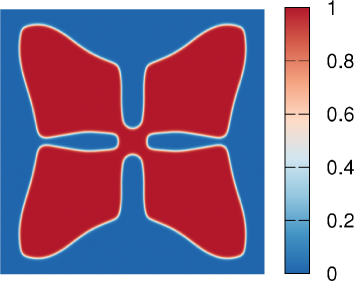
(a)

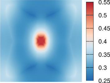
(b)

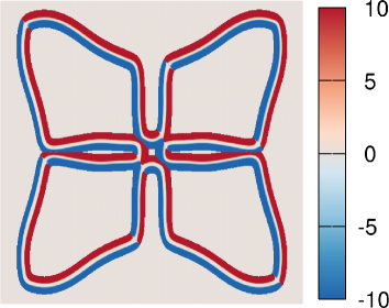
(c)

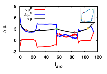
(d)

Figure 7: (a) Order parameter map in $(110)$ plane section at $t=1100$ (b) Shift in chemical potential ($\Delta\mu^{*}$) map corresponding to order parameter map (c) curvature map corresponding to the order parameter map (d) The variation of shift in chemical potential ($\Delta\mu$) as a function of arc-length. The inset shows the one-fourth section of the contour profile in $(110)$ plane. The coloured dots on the interface contour are shown in the inset, and the corresponding values of $\Delta\mu$ are shown by the same coloured dots.

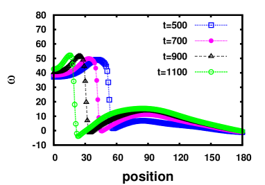
(a)

(b)

Figure 8: (a) $\omega$ profiles along $[001]$ direction at simulation times $t=500$, $700$, $900$, $1100$ $\mathrm{s}$. The value of $\omega$ in the precipitate increases with time. (b) The temporal evolution of $\Delta\omega=\omega^{\upalpha}-\omega^{\upbeta}$ across the interface along $[001]$ direction. The $\Delta\omega$ increases after initial decrease which suggests temporal increment in contribution to the chemical potential.

In addition, we track the evolution of velocity of the interface $v_{\textrm{g}}$ along $[001]$ direction and $\Delta\mu$ in the matrix ahead of the interface along $[001]$ direction. Fig. 9(a) shows the evolution of position of the interface $l_{\textrm{g}}$ along $[001]$ direction which increases initially and further linearly decreases until the pinch-off takes place. The linear decrease in $l_{\textrm{g}}$ occurs when the grooves develop and interface along $[001]$ advances towards the centre of the precipitate. As a result, the $v_{\textrm{g}}$ initially increases and reaches a steady state value when the interface starts advancing towards the centre of the precipitate. Fig. 9(c) shows the evolution of $\mu_{\textrm{g}}$ as a function of time. The value of $\mu_{\textrm{g}}$ initially decreases and begin to increase as soon as the groove forms along the $[001]$ direction. The temporal increment of $\mu_{\textrm{g}}$ signifies the precipitate dissolution along $[001]$ direction. Two-dimensional simulation show similar trends of temporal evolution of $l_{\textrm{g}}$, $v_{\textrm{g}}$, and $\mu_{\textrm{g}}$ (see Figs. 11(a), 11(b), and 11(c)). On the contrary, when only anisotropy in interfacial energy is present, the $l_{\textrm{g}}$ continues to increase with time as shown in Fig. 10(a). The velocity of the interface along $[01]$ direction reaches a negative steady state values (close to zero) which indicates the movement of interface along $[01]$ direction away from the centre of the precipitate (see Fig. 10(b)). After the initial transient, $\mu_{\textrm{g}}$ continues to decrease having negative values (see Fig. 10(c)). The negative values of $\mu_{\textrm{g}}$ suggest growth of the interface along $[10]$ direction.

(a)

(b)

(c)

Figure 9: (a) The evolution of distance of interface from the centre of precipitate ($l_{\textrm{g}}$) along $[001]$ direction. The $l_{\textrm{g}}$ decreases linearly with time. (b) The evolution of velocity $v_{\textrm{g}}$ of the interface along $[001]$ direction as a function of time. The $v_{\textrm{g}}$ reaches a steady-state over time before the pinch off takes place. (c) Temporal evolution of $\mu_{\textrm{g}}$ along $[001]$ direction. After the initial decrease, the value of $\mu_{\textrm{g}}$ tends to increase suggesting precipitate dissolution along $[001]$ direction.

(a)

(b)

(c)

Figure 10: (a) The evolution of distance of interface from the center of precipitate ($l_{\textrm{g}}$) along $[01]$ direction. The $l_{\textrm{g}}$ increases with time. (b) The evolution of velocity $v_{\textrm{g}}$ of the interface along $[01]$ direction as a function of time. The $v_{\textrm{g}}$ achieves a negative steady-state values over time. (c) Temporal evolution of $\mu_{\textrm{g}}$ along $[01]$ direction. After the initial transient, the $\mu_{\textrm{g}}$ tends to decrease with negative value which suggests advancement of interface along $[01]$ direction away from the center of the precipitate. Here the ratio of interfacial energy along $[11]$ direction to that along $[10]$ direction is $1.25$.

(a)

(b)

(c)

Figure 11: (a) The evolution of distance of interface from the center of precipitate ($l_{\textrm{g}}$) along $[01]$ direction. The $l_{\textrm{g}}$ decreases with time after achieving a maximum value. (b) The evolution of velocity $v_{\textrm{g}}$ of the interface along $[01]$ direction as a function of time. The $v_{\textrm{g}}$ achieves a positive steady-state values over time. (c) Temporal evolution of $\mu_{\textrm{g}}$ along $[01]$ direction. The $\mu_{\textrm{g}}$ tends to increase which suggests advancement of interface along $[01]$ direction towards the center of the precipitate.

3.4 Effects of lattice misfit

In this section, we discuss the effects of lattice misfit on the initiation of splitting instability. To understand the effect of lattice misfit, we choose different combinations of supersaturation ($c_{\infty}=$ $25\%$, $35\%$, $45\%$) and lattice misfit ($\epsilon^{*}=$ $0.75\%$, $0.85\%$ and $1\%$). For all cases, the elastic energy anisotropy is $4$. Table. 4 shows the precipitate morphologies at the same simulation time $t=10000$ for different levels of lattice misfit and supersaturations. At all given levels of lattice misfit and supersaturation, due to the point effect of diffusion, precipitate develops concavities, however, only at higher misfit and supersaturation concavities transform to grooves and lead to splitting of the precipitate.

	$c_{\infty}=25\%$	$c_{\infty}=35\%$	$c_{\infty}=45\%$
$\epsilon^{*}=0.5\%$
$\epsilon^{*}=0.75\%$
$\epsilon^{*}=0.85\%$
$\epsilon^{*}=1\%$

Table 4: Precipitate morphologies at different levels of lattice misfit $\epsilon^{*}=0.5\%$, $0.75\%$, $0.85\%$, $1\%$ and supersaturation $c_{\infty}=25\%$, $35\%$, $45\%$ at the same simulation time of $10000$. Here, the Zener anisotropy parameter is $4$. A combination of higher misfit and supersaturation promotes splitting instability

At $\epsilon^{*}=0.5\%$, for all given supersaturations, the precipitate do not transform to form split pattern. As the lattice misfit is increased to $0.75\%$ when the supersaturation is $45\%$, grooves develop and further precipitate coalesce to form a hollow precipitate with matrix phase at the core. Similar phenomenon occurs when lattice misfit is $1\%$ and supersaturation is $c_{\infty}=35\%,45\%$. Fig. 12(a),  12(b), and 12(c) show the isosurface representation of the precipitate morphology at $c_{\infty}=45$ and $\epsilon^{*}=0.75\%$, $c_{\infty}=35\%$ and $\epsilon^{*}=1\%$, $c_{\infty}=45\%$ and $\epsilon^{*}=1\%$, respectively at the same time $t=10000$. The corresponding plane section of precipitate morphology in $(110)$ plane clearly shows the matrix phase trapped inside the precipitate (see Fig. 12(d), 12(e), and 12(f)).

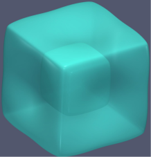
(a)

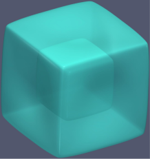
(b)

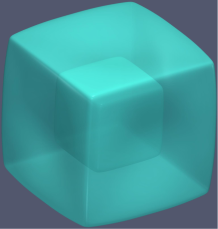
(c)

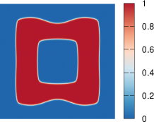
(d)

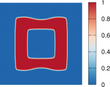
(e)

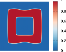
(f)

Figure 12: Isosurface representation at time $t=10000$ for (a) supersaturation $45\%$, $35\%$ and lattice misfit $0.75\%$ (b) supersaturation $35\%$ and lattice misfit $1\%$, and (c) supersaturation $45\%$ and lattice misfit $1\%$.

To understand how matrix phase get trapped inside the precipitate, we track the temporal evolution of precipitate morphology in $(110)$ plane. Table 5 shows the temporal evolution of precipitate morphology, where precipitate arms coalesce along $\langle 110\rangle$ directions due to which matrix phase gets trapped by the precipitate phase. The precipitate-matrix interface along $\langle 110\rangle$ directions (one which is closer to the center of the precipitate) continues to advance towards the center of the precipitate leading to pinch-off of the primary arms. Later, the grooves along $\langle 100\rangle$ directions start closing, and the final morphology is a hollow precipitate with matrix phase at the center as shown in Fig. 12. However, for lattice misfit $1\%$ and $c_{\infty}=45\%$, although initially the matrix phase appears at the center of the precipitate, the coalescence of the arms takes place and entrapment of matrix occurs. Subsequently, the hollow precipitate forms where cuboidal matrix phase is trapped at the center.

When the lattice misfit is $0.85\%$ and $0.75\%$ for $c_{\infty}=45\%$ and $c_{\infty}=35\%$, respectively, the Euler characteristics are equal to two at the initial stages. Afterward, the Euler characteristics shoot up to $16$ which corresponds to the disjoint union of eight precipitates. On the other hand, for lattice misfit of $0.5\%$ and supersaturation of $25\%$, the Euler characteristics ($\chi=2$) remains unchanged throughout the evolution. In other case ($c_{\infty}=45\%$ and $\epsilon^{*}=1\%$), initially the Euler characteristic of $4$ goes down to $-20$ and further jumps up to $-8$. The negative value of $\chi$ suggests the presence of packets of matrix phase entrapped inside the precipitate. Although at the initial stage, the matrix phase forms at the center of precipitate due to the instability, during the process of groove running towards the center of precipitate, the secondary arms of the precipitate impinge which results in entrapment of the matrix phases. In the late stage, the Euler characteristics achieve a value of four which indicates a morphology where cuboidal matrix phase is entrapped by the cuboidal precipitate (see table LABEL:tab:TopoPrecipitateEvolve).

	$t=200$	$t=400$	$t=1800$	$t=10000$
Isosurface view
Composition map
Order Parameter map

Table 5: Temporal evolution of the precipitate morphology at time $t=200,\,400,\,1800,\,10000$. First row shows the isosurface representation of precipitate morphology. Second row shows the composition map in $(110)$ plane passing through the centre of the simulation box, and third row shows the corresponding order parameter map. Here, $c_{\infty}=45\%$ and $\epsilon^{*}=0.75\%$.

Fig. 13(a) shows the temporal evolution of the $\mu_{\textrm{g}}$ along $[001]$ direction for different lattice misfits $0.5\%$, $0.75\%$, and $0.85\%$ at $c_{\infty}=45\%$. Fig. 13(b) depicts the temporal evolution of $v_{\textrm{g}}$ along $[001]$ direction corresponding to the same levels of lattice misfit. The values of $\mu_{\textrm{g}}$ initially decrease at all levels of lattice misfit, however, for higher misfit ($\epsilon^{*}=0.85\%$, and $0.75\%$) it continues to increase further with time. At the lattice misfit $0.5\%$, $\mu_{\textrm{g}}$ continues to decrease in contrast to the cases of lattice misfits $0.75\%$ and $0.85\%$. An increment in $\mu_{\textrm{g}}$ suggests precipitate dissolution along $[001]$ direction. For all the levels of lattice misfit, the $v_{\textrm{g}}$ achieves a steady state. However, higher lattice misfit ($\epsilon^{*}=0.85\%$ and $0.75\%$) have positive values of velocity at a steady state suggesting the movement of the interface towards the center of the precipitate. Whereas, in the case of lattice misfit $0.5\%$, the steady state value of velocity is negative which suggests the movement of the interface away from the centre of the precipitate along $[001]$ direction.

Moreover, we plot the variation of elastic stress and curvature contribution to the shift in chemical potential as a function of arc-length. Figs. 14 and 15 represent the variation of $\Delta\mu^{\mathrm{el}}$ and $\Delta\mu^{\mathrm{K}}$ with arc-length for lattice misfits of 0.75% and 0.5% at simulation time $t=1400$. Similar to the case of lattice misfit of $0.85\%$ (see Fig. 7(d)), the values of $\Delta\mu^{\mathrm{el}}$ are higher in the region left to the red point and right to the yellow point (i.e. grooves oriented along $\langle 100\rangle$ and $\langle 110\rangle$). On the hand, for the case of lattice misfit of 0.5%, the $\Delta\mu$ value is the highest near the green dot due to which concavities present along $\langle 100\rangle$ and $\langle 110\rangle$ directions tend to vanish. With the decrease in misfit, the contribution of elastic stress to the shift in chemical potential decreases and thereby the point effect of diffusion subsides. As a result, the capillary forces kick in early during the evolution of precipitate morphology, and precipitate restores the cuboidal morphology by removing the concavities.

(a)

(b)

Figure 13: (a) Temporal evolution of chemical potential ($\mu_{\textrm{g}}$) of matrix ahead of interface along $[001]$ at different levels of lattice misfit. At higher lattice misfit ($\epsilon^{*}=0.85\%$, and $0.75\%$), $\mu_{\textrm{g}}$ continues to increase once reached the lowest value. Whereas, at $\epsilon^{*}=0.5\%$, $\mu_{\textrm{g}}$ continues to decrease. The increase in $\mu_{\textrm{g}}$ suggests precipitate dissolution along $[001]$. (b) Temporal evolution of velocity ($v_{\textrm{g}}$) of the interface along $[001]$ direction for different levels of lattice misfit. At lattice misfit of 0.5%, $v_{\textrm{g}}$ have negative steady state values, whereas other cases have positive steady state values. The positive values of $v_{\textrm{g}}$ suggest movement of the interface towards the center of the precipitate. Here, Zener anisotropy parameter is 4 and supersaturation is 45%.

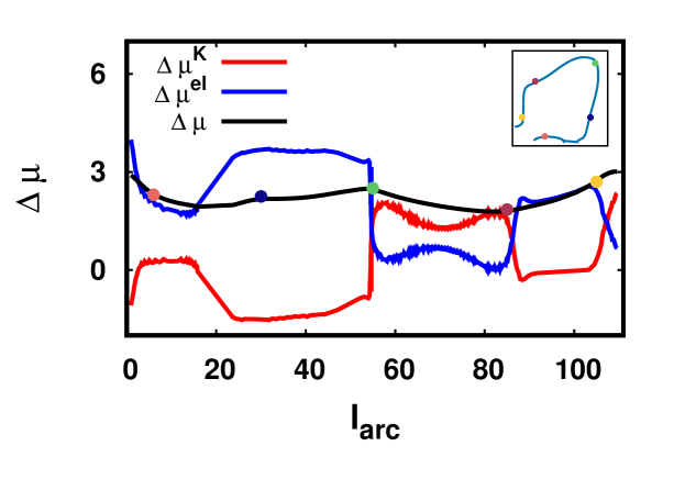
Figure 14: Variation of shift in chemical potential due to curvature ($\Delta\mu^{\textrm{K}}$) and elastic stresses ($\Delta\mu^{\textrm{el}}$) as a function of arc-length at time $t=1400$. Here, supersaturation is 45% and lattice misfit is 0.75%

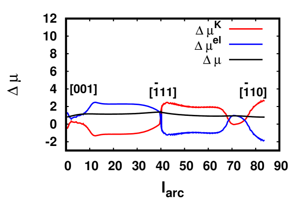
Figure 15: Variation of shift in chemical potential due to curvature ($\Delta\mu^{\textrm{K}}$) and elastic stresses ($\Delta\mu^{\textrm{el}}$) as a function of arc-length at time $t=1400$. Here, supersaturation is 45% and lattice misfit is 0.5%

3.5 Effects of anisotropy in elastic energy

In this section, we discuss the effects of anisotropy in elastic energy on the initiation of particle splitting instability. We choose Zener anisotropy parameter of $2$, $3$, and $4$, lattice misfit of $0.5\%$, $0.75\%$, and $0.85\%$, and supersaturation of $45\%$. Table 6 shows the precipitate morphologies at a same simulation time of $1000$ for different levels of lattice misfit and Zener anisotropy parameter. At all combinations of lattice misfit and Zener anisotropy parameter, the dendritic instability grows, however, higher lattice misfit promotes particle splitting.

	$A_{\textrm{z}}=2$	$A_{\textrm{z}}=3$	$A_{\textrm{z}}=4$
$\epsilon^{*}=0.5\%$
$\epsilon^{*}=0.75\%$
$\epsilon^{*}=0.85\%$

Table 6: Precipitate morphologies for different levels of elastic misfit $\epsilon^{*}=0.5\%,0.75\%,0.85\%$ and elastic energy anisotropy $A_{\textrm{z}}=2$, $3$, $4$ at time $t=10000$. Here, supersaturation is 45%. A higher value of lattice misfit promotes splitting instability

At a lattice misfit of 0.85%, for $A_{\textrm{z}}=4.0$ and $3.0$, the precipitate show split patterns, whereas for $A_{\textrm{z}}=2.0$, hollow cuboidal precipitate forms. As discussed in the previous section, at $A_{\textrm{z}}=2.0$, the precipitate coalesces along $\langle 110\rangle$ directions; matrix phase gets trapped within precipitate phase and further pinch-off takes place.

Figs. 16(a) and 16(b) represents the temporal evolution of $\mu_{\textrm{g}}$ and $v_{\textrm{g}}$ along $[001]$ direction respectively. The values of $\mu_{\textrm{g}}$ tends to increase with time, whereas the values of $v_{\textrm{g}}$ achieve a positive steady state value for all levels of Zener anisotropy parameter at supersaturation of 45% and lattice misfit of 0.85%. As discussed in the previous section, the temporal increment in $\mu_{\textrm{g}}$ suggests precipitate dissolution along the $[001]$ direction.

(a)

(b)

Figure 16: (a) Temporal evolution of chemical potential ($\mu_{\textrm{g}}$) of matrix ahead of interface along $[001]$ at different levels of Zener anisotropy parameter. At all levels of Zener anisotropy parameter, $\mu_{\textrm{g}}$ tends to increase. The increase in $\mu_{\textrm{g}}$ suggests precipitate dissolution along $[001]$ direction. (b)Temporal evolution of velocity ($v_{\textrm{g}}$) of the interface along $[001]$ direction for different levels degree of elastic energy anisotropy. At all levels of Zener anisotropy parameter, $v_{\textrm{g}}$ achieve a positive steady state value. The positive values of $v_{\textrm{g}}$ suggest movement of the interface towards the center of the precipitate. Here, lattice misfit is 0.85% and supersaturation is 45%.

Figs. 17 and 18 shows the variation of shift in chemical potential $\Delta\mu$ for $A_{\textrm{z}}=3$ and $A_{\textrm{z}}=2$ respectively at a same simulation time of $1400$. At $A_{\textrm{z}}=3.0$, the shift in chemical potential are higher at regions along $[\bar{1}10]$, $[\bar{1}11]$, and $[001]$ directions. Similar variation is observed for the case of $A_{\textrm{z}}=2.0$.

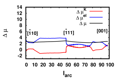
Figure 17: Variation of shift in chemical potential due to curvature ($\Delta\mu^{\textrm{K}}$) and elastic stresses ($\Delta\mu^{\textrm{el}}$) as a function of arc-length at time $t=1400$ for $A_{\textrm{z}}=3.0$. Here, supersaturation is 45% and lattice misfit is 0.85%.

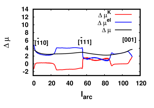
Figure 18: Variation of shift in chemical potential due to curvature ($\Delta\mu^{\textrm{K}}$) and elastic stresses ($\Delta\mu^{\textrm{el}}$) as a function of arc-length at time $t=1400$ for $A_{\textrm{z}}=2.0$. Here, supersaturation is 45% and lattice misfit is 0.5%

3.6 Effects of particle interactions

Experimental reports show that, unlike solid-state dendrites, split patterns are observed even when particles are closely spaced during isothermal heat treatments [16]. Hence, we discuss the effects of particle interactions on the particle splitting instability. Here, we perform two-dimensional simulations with a box size having $4096\times 4096$ grid points and grid spacing of $0.2$. We begin the simulation with two particles having centers at $\displaystyle\left(\frac{nx\times dx}{2},\frac{ny\times dy}{4}\right)$ and $\displaystyle\left(\frac{nx\times dx}{2},\frac{3ny\times dy}{4}\right)$. We assume supersaturation of 25%, lattice misfit of 0.85% and Zener anisotropy parameter of 4. Fig. 19 depicts the evolution of two particle microstructure which results in the formation of doublets. Initially, both the particles develop dendrite-like structure with predominant growth along $\langle 11\rangle$ directions. Further, grooves develop on the particles along $\langle 10\rangle$ directions. During the further evolution of microstructure, as the particles start interacting with each other, grooves along $[01]$ direction tends to vanish and grooves along $[10]$ are promoted to advance towards the centers of the precipitates. Later, the microstructure evolves to form the doublets oriented along $[10]$ direction.

(a) t=1

(b) t=10000

(c) t=20000

(d) t=40000

(e) t=50000

(f) t=200000

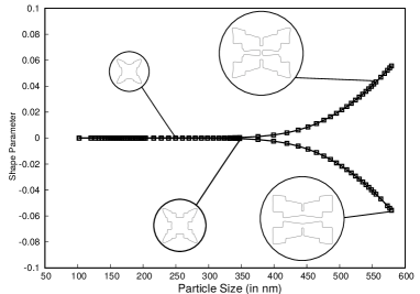
(g) Bifurcation diagram showing T$\rightarrow$O transition

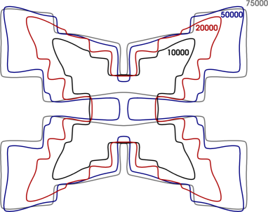
(h) Contours of the particle at various timesteps

Figure 19: Evolution of precipitates to the formation of doublets due to interaction of two particles oriented along $[01]$ direction. The particle splits in the direction perpendicular to the direction of particle orientation. Here, supersaturation is $25\%$ and misfit is $0.85\%$.

Fig. 20(b) shows the temporal evolution of $v_{\textrm{g}}$ along $[10]$ and $[01]$ directions. Following the initial equal values of velocity for both the directions, $v_{\textrm{g}}$ along $[10]$ direction achieves a maximum value and decrease further before the split patterns form. On the other hand, $v_{\textrm{g}}$ along $[01]$ direction achieves a smaller positive value and further decreases to a negative value.

Fig. 20(c) depicts the temporal evolution of the chemical potential in the matrix ahead of the interface along $[10]$ and $[01]$ directions. The initial same values of $\mu_{\textrm{g}}$ along $[10]$ and $[01]$ directions succeeds the increment in the values of $\mu_{\textrm{g}}$ along $[10]$ direction. On the other hand, the values of $\mu_{\textrm{g}}$ along $[01]$ direction keep on decreasing with time. A preference to increment in $\mu_{\textrm{g}}$ along $[10]$ direction results in doublets oriented along $[10]$ direction.

(a)

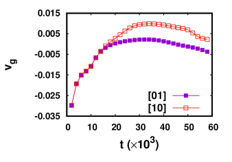
(b)

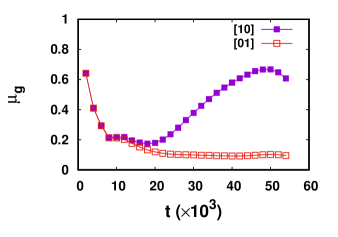
(c)

Figure 20: (a) Temporal evolution of $l_{\textrm{g}}$ along $[10]$ and $[01]$ directions. The interface along $[10]$ direction continues to advance towards the centre of the precipitate. (b) Temporal evolution of $v_{\textrm{g}}$ along $[10]$ and $[01]$ directions of the precipitate. Initially, both the velocities are negative and equal. Further, the velocity along $[10]$ achieves a positive value, whereas velocity along $[01]$ achieves a negative value. (c) Temporal evolution of $\mu_{\textrm{g}}$ along $[10]$ and $[01]$ directions of the precipitate. After the initial equal values for both directions, the $\mu_{\textrm{g}}$ along $[10]$ direction tends to grow with time which suggests precipitate dissolution.

3.7 Discussion

We presented simulation results of precipitate growth at different levels of lattice misfit, supersaturation and elastic anisotropy in three dimensions. Simulation results indicate that the variation of lattice misfit, supersaturation, elastic anisotropy and interfacial energy anisotropy influences the formation of split patterns. Anisotropies in elastic energy and interfacial energy promote morphological instability, however, only anisotropy in elastic energy promotes the pinch-off instability. Thus, particle splitting is an elastically driven instability where dendritic structure is a prerequisite.

We observe that the precipitate develops primary dendritic arms along $\{111\}$ (in 3D) and $\{11\}$ directions (in 2D) before the precipitate splits into eight or four smaller precipitates. Three distinct precipitate morphologies are observed in three-dimensions, namely (i) No split pattern (NSP) (ii) Split pattern (SP) (iii) Trap split pattern (TSP). NSP represents the case where precipitate develops primary arms during the initial stages of growth, however the precipitate restores to cuboidal shape (e.g. refer to precipitate morphology for $c_{\infty}=25\%$ and $\epsilon^{*}=0.85\%$ in Table 4). SP corresponds to the case where a single precipitate grows to form eight smaller cuboidal precipitates via formation of dendritic structure with primary arms along $\{111\}$ crystallographic directions and concavities along $\{100\}$ and $\{110\}$ crystallographic directions (refer to precipitate morphology for $c_{\infty}=35\%$ and $\epsilon^{*}=0.75\%$ in Table 4). Trap split pattern represents a precipitate morphology where precipitate phase entraps the matrix phase (refer to precipitate morphology $c_{\infty}=45\%$ and $\epsilon^{*}=1\%$ in Table 4). In case of two-dimensional simulations, we only observe split patterns. In his classical monograph, Doi et al. [1] explained the splitting phenomenon based on bifurcation theory wherein elastic interaction energy modulates the precipitate to form smaller octet or quartet split patterns. By taking into consideration the work of Doi et al., we rationalize our results by plotting elastic free-energy density and interfacial free-energy density.

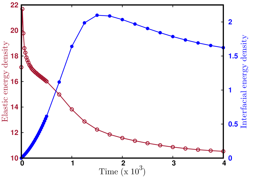
(a)

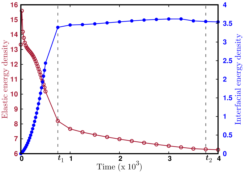
(b)

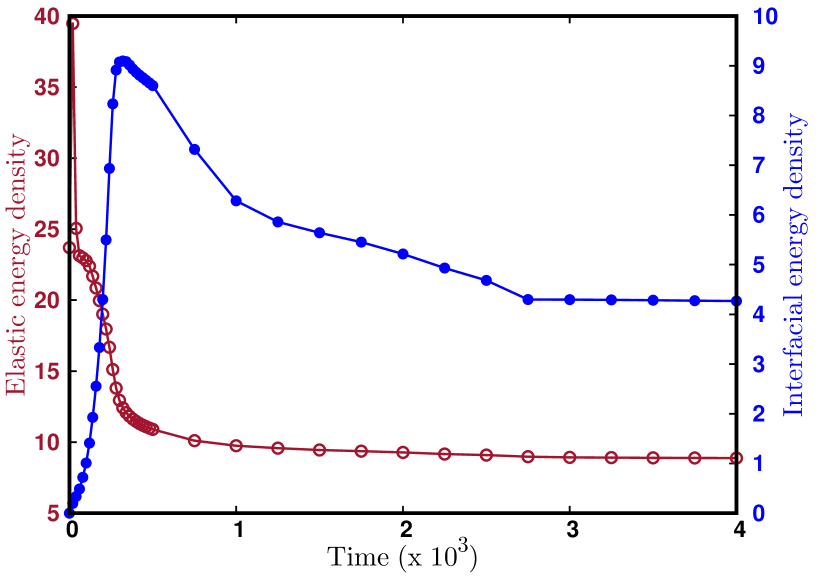
(c)

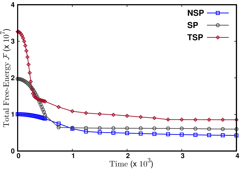
(d)

Figure 21: (a) Temporal variation of elastic energy density and interfacial energy density for (a) $c_{\infty}=25\%$, $A_{\textrm{z}}=4$ and $\epsilon^{*}=0.85\%$. (b) $c_{\infty}=35\%$, $A_{\textrm{z}}=4$ and $\epsilon^{*}=0.75\%$ (c) $c_{\infty}=45\%$, $A_{\textrm{z}}=4$ and $\epsilon^{*}=1\%$. (d) Corresponding temporal evolution of total free-energy $\mathcal{F}$

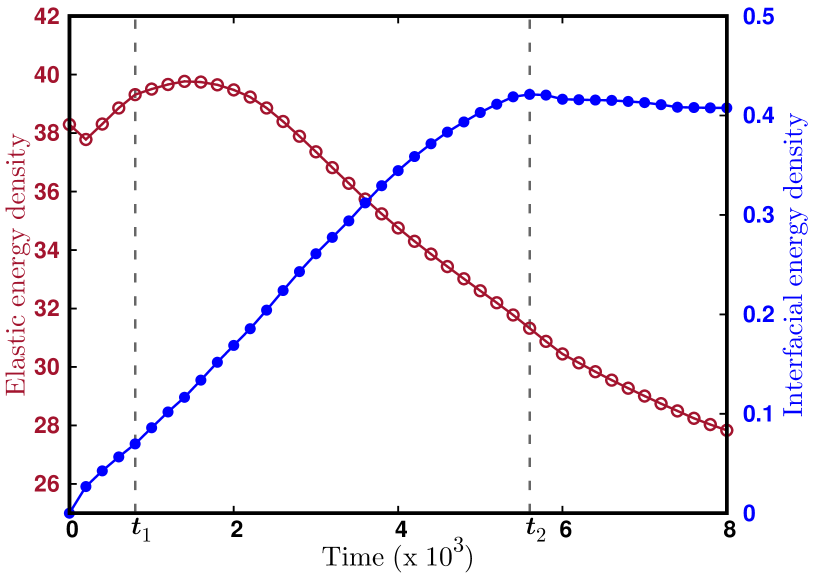
(a)

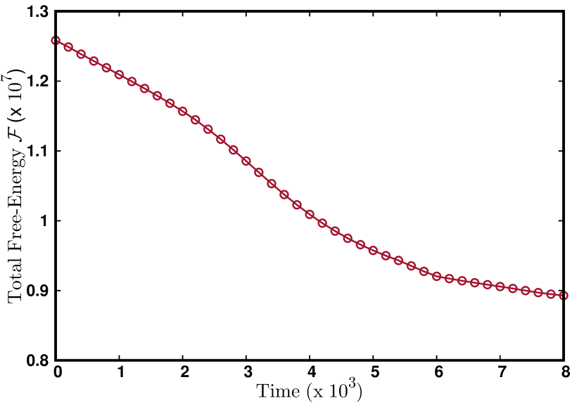
(b)

Figure 22: (a) Temporal variation of elastic energy density and interfacial energy density for $c_{\infty}=25\%$, $A_{\textrm{z}}=4$ and $\epsilon^{*}=1\%$. $t_{1}$ represents the initiation of grooving, and $t_{2}$ denotes the time of pinch-off. (b) Corresponding temporal evolution of total free-energy $\mathcal{F}$

Fig. 21(a), 21(b) and 21(c) depict the evolution of elastic free-energy density and interfacial free-energy density for NSP, SP and TSP respectively. Fig. 21(d) represents the temporal evolution of total free-energy for NSP, SP and TSP cases. For all cases, the total energy of the system decreases monotonically. However, within time intervals $t_{1}$ and $t_{2}$ the interfacial energy density continuous to increase, whereas elastic energy density after attaining a peak value continually drop (see Fig. 21(b)). Likewise, we observe inverse behavior of elastic free-energy density and interfacial free-energy density for 2D simulations of split patterns (see Fig. 22). Thus, reduction in the elastic free-energy density driven by increasing elastic interaction energy contribution concomitant with the increase in interfacial free-energy density promotes the process of grooving which finally results in split pattern. On the contrary, the concomitant decrement in the elastic free-energy density and interfacial free-energy density promotes the elimination of concavities or grooves which results in single cuboidal morphology (NP). TSP is a peculiar case where the process of elimination of concavities by merging of primary arms and pinch-off at the center of precipitate occur. Initially elastic free-energy density and interfacial free-energy density have inverse relationship until interfacial energy attains a peak. Post peak value of interfacial energy suggests a process of merging of primary arms, whereas grooves continues to advance towards the center of the precipitate. The decrease in the interfacial free-energy is not continuous, rather with intermittent temporal change in slope.

Doi  [1, 2] calculated the elastic interaction energy for a pair of ellipsoidal $\gamma^{\prime}$ particles as a function of distance between them and alignment directions $\langle hkl\rangle$. The analysis calculation the negative minimum for elastic interaction energy when two particles are aligned along $\langle 100\rangle$. On the similar manner, we evaluated the elastic interaction energy for a configuration in two-dimensions as shown in Fig. 23(a). The configuration has a pair of cuboidal $\gamma^{\prime}$ precipitates of equal size in a box of dimensions $L_{x}\times L_{y}$ such that $L_{x},L_{y}>>R_{sep}$, where $R_{sep}$ denotes the distance between centers of $\gamma^{\prime}$ precipitates. The elastic interaction energy $\mathcal{F}^{\prime}_{el}$ for a pair of precipitates is evaluated as

$$\mathcal{F}^{\prime}_{el}=\mathcal{F}_{el}-2\mathcal{F}_{self},$$ (49)

where $\mathcal{F}_{el}$ is the total elastic energy and $\mathcal{F}_{self}$ is the self elastic energy of a single precipitate. Fig. 23(b) shows the variation of elastic interaction energy for a pair of cuboidal precipitates aligned along $[100]$ direction as a function of $R_{sep}$. We notice that the variation of $\mathcal{F}^{\prime}_{el}$ shows a minimum at $R_{sep}^{min}\approx 25nm$ which suggests the tendency for a pair of precipitates to remain separated at $R_{sep}^{min}$ and aligned along $\langle 100\rangle$. We fit the elastic interaction energy data points to a even polynomial in terms of $1/R_{sep}$ of degree twelve:

$$\mathcal{F}^{\prime}_{fit}=\sum_{i=0}^{i=6}\left(\frac{a_{i}}{R_{sep}^{2i}}\right),$$ (50)

where $a_{i}$ represent the coefficients of the polynomial. The fitted curve of the polynomial is presented in Fig. 23(b).

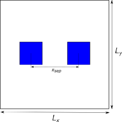
(a)

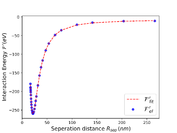
(b)

Figure 23: (a) Schematic representatin of configuration showing arrangement of pair of cuboidal misfitting precipitate in a matrix (b) Variation of elastic interaction energy $F_{el}^{int}$ as a function of separation distance ($R_{sep}$) along $[100]$ direction.

4 Conclusion

We present a diffuse-interface model which can recover the conditions of interfacial equilibrium for a curved elastically stressed interface. We have performed three-dimensional as well as two-dimensional phase-field simulations of particle splitting where dendrite-like structure leads to particle splitting. Our results show that the presence of elastic anisotropy and lattice misfit is necessary for splitting. Anisotropy in interfacial energy do not lead to splitting of precipitate. Hence, particle splitting is an elastically induced phenomenon. The splitting occurs when the contribution of elastic stresses is higher as compared to curvature along $\langle 110\rangle$ and $\langle 100\rangle$ directions ($\langle 10\rangle$ in two-dimensions). Particles in proximity can restrict the growth of grooves in certain direction and doublet can form. Finite size effects result in formation of plate shaped precipitates which compare well with the bifurcation theories.

Appendix A Gradient energy density

The gradient free energy density $f_{\textrm{grad}}$ of the system is written as:

$$f_{\textrm{grad}}(\nabla\phi)=\varepsilon^{2}|\nabla\phi|^{2}+\Gamma_{\langle hkl\rangle}|\Delta\phi|^{2},$$ (51)

where $\varepsilon^{2}$ is the gradient free energy coefficient, $\Gamma_{\langle hkl\rangle}$ is the fourth-rank gradient tensor which incorporates anisotropy in the interfacial energy. The fourth-rank gradient tensor reads as

$$\Gamma_{\langle hkl\rangle}=\Gamma_{\textrm{A}}(h^{4}+k^{4}+l^{4})+\Gamma_{\textrm{I}},$$ (52)

where $\Gamma_{\textrm{A}}$ and $\Gamma_{\textrm{I}}$ denote the anisotropic and isotropic components of the fourth-rank gradient energy tensor, and $h$,$k$,$l$ represent the direction cosines of normal to the interface. The interfacial energy of the system must be non-negative, as a result the following constraints must be valid:

$$\Gamma_{\textrm{I}} \geq \lvert\Gamma_{\textrm{A}}\rvert\quad\forall\;\;\Gamma_{\textrm{A}}\leq 0,$$ (53)

$$-\Gamma_{\textrm{I}} \leq \frac{\Gamma_{\textrm{A}}}{3}\;\quad\forall\;\;\Gamma_{\textrm{A}}>0.$$ (54)

When $\Gamma_{\textrm{A}}<0$, the values of $\Gamma_{\langle hkl\rangle}$ are maximum along $\langle 111\rangle$ directions and minimum along $\langle 100\rangle$ directions. Consequently, interfacial energy along $\langle 100\rangle$ will be lower than that along $\langle 111\rangle$ directions. Hence, the Wulff shape will have facets along $\langle 100\rangle$ directions. On the other hand, when $\Gamma_{\textrm{A}}>0$, $\Gamma_{\langle hkl\rangle}$ possesses maximum values along $\langle 100\rangle$ directions and minimum along $\langle 111\rangle$ directions. Hence, the Wulff shape will exhibit facets along $\langle 111\rangle$ directions. We choose the earlier case for our study to show the effect of interfacial energy anisotropy.

Appendix B Elastic driving force

The elastic-free energy density is expressed as

$$f^{\mathrm{el}} = \frac{1}{2}C_{ijkl}(\mathbf{r})[\delta\epsilon_{ij}(\mathbf{r})+\bar{\epsilon}_{ij}-\epsilon_{ij}^{*}(\mathbf{r})][\delta\epsilon_{kl}(\mathbf{r})+\bar{\epsilon}_{kl}-\epsilon_{kl}^{*}(\mathbf{r})]$$ (55)

$$= \frac{1}{2}\left[C_{ijkl}^{0}+C_{ijkl}^{\prime}\left(2h(\phi)-1\right)\right]\left[\delta\epsilon_{ij}(\mathbf{r})+\bar{\epsilon}_{ij}-\epsilon^{0}\delta_{ij}h(\phi)\right]\left[\delta\epsilon_{kl}(\mathbf{r})+\bar{\varepsilon}_{kl}-\epsilon^{0}\delta_{ij}h(\phi)\right]$$

Taylor expansion of elastic free-energy density about $f^{\mathbf{el}}$ derives as

$$f^{\mathrm{el}}+\delta f^{\mathrm{el}}=\frac{1}{2} \left[C_{ijkl}^{0}+C_{ijkl}^{\prime}\left(2h(\phi)-1\right)+2C_{ijkl}^{\prime}h^{\prime}(\phi)\delta\phi\right]$$ (56)

$$\left[\delta\epsilon_{ij}(\mathbf{r})+\bar{\varepsilon}_{ij}-\epsilon^{0}\delta_{ij}h(\phi)-\epsilon^{0}\delta_{ij}h^{\prime}(\phi)\delta\phi\right]$$

$$\left[\delta\epsilon_{kl}(\mathbf{r})+\bar{\epsilon}_{kl}-\epsilon^{0}\delta_{kl}h(\phi)-\epsilon^{0}\delta_{kl}h^{\prime}(\phi)\delta\phi\right]$$

Further simplification leads to

$$\delta f^{\mathrm{el}}= -\frac{1}{2}C_{ijkl}(\mathbf{r})\left[\delta\epsilon_{ij}(\mathbf{r})+\bar{\epsilon}_{ij}-\epsilon^{0}\delta_{ij}h(\phi)\right]\epsilon^{0}\delta_{kl}h^{\prime}(\phi)\delta\phi$$ (57)

$$-\frac{1}{2}C_{ijkl}(\mathbf{r})\left[\delta\epsilon_{kl}(\mathbf{r})+\bar{\epsilon}_{kl}-\epsilon_{kl}^{0}h(\phi)\right]\epsilon^{0}\delta_{ij}h^{\prime}(\phi)\delta\phi$$

$$+\frac{1}{2}C_{ijkl}(\mathbf{r})\left[\epsilon^{0}\epsilon^{0}\delta_{ij}\delta_{kl}(h^{\prime}(\phi))^{2}(\delta\phi)^{2}\right]$$

$$+C^{\prime}_{ijkl}h^{\prime}(\phi)\delta\phi\left[\delta\epsilon_{ij}(\mathbf{r})+\bar{\epsilon}_{ij}-\epsilon^{0}\delta_{ij}h(\phi)\right]\left[\delta\epsilon_{kl}(\mathbf{r})+\bar{\epsilon}_{kl}-\epsilon^{0}\delta_{kl}h(\phi)\right]$$

$$-C_{ijkl}^{\prime}h^{\prime}(\phi)\delta\phi\left[\delta\epsilon_{ij}(\mathbf{r})+\bar{\epsilon}_{ij}-\epsilon^{0}\delta_{ij}h(\phi)\right]\epsilon^{0}\delta_{kl}h^{\prime}(\phi)\delta\phi$$

$$-C^{\prime}_{ijkl}h^{\prime}(\phi)\delta\phi\left[\delta\epsilon_{kl}(\mathbf{r})+\bar{\epsilon}_{kl}-\epsilon^{0}\delta_{kl}h(\phi)\right]\epsilon^{0}\delta_{ij}h^{\prime}(\phi)\delta\phi$$

$$+C^{\prime}_{ijkl}h^{\prime}(\phi)\delta\phi\left[\epsilon^{0}\epsilon^{0}(h^{\prime}(\phi))^{2}(\delta\phi)^{2}\right]\delta_{ij}\delta_{kl}$$

Considering only first-order terms in $\delta\phi$ and neglecting higher-order terms in $\delta\phi$,

$$\delta f^{\mathrm{el}}=\frac{1}{2}\Big{[} 2C^{\prime}_{ijkl}h^{\prime}(\phi)\delta\phi\left[\delta\epsilon_{ij}(\mathbf{r})+\bar{\epsilon}_{ij}-\epsilon^{0}\delta_{ij}h(\phi)\right]\left[\delta\epsilon_{kl}(\mathbf{r})\bar{\epsilon}_{kl}-\epsilon^{0}\delta_{kl}h(\phi)\right]$$ (58)

$$-C_{ijkl}\left[\delta\epsilon_{ij}(\mathbf{r})+\bar{\epsilon}_{ij}-\epsilon^{0}\delta_{ij}h(\phi)\right]\epsilon^{0}\delta_{kl}h^{\prime}(\phi)\delta\phi$$

$$-C_{ijkl}\left[\delta\epsilon_{kl}(\mathbf{r})+\bar{\epsilon}_{kl}-\epsilon^{0}\delta_{kl}h(\phi)\right]\epsilon^{0}\delta_{ij}h^{\prime}(\phi)\delta\phi\Big{]}$$

Invoking symmetries of $C_{ijkl}$, the elastic driving force is expressed as

$$\frac{\delta f^{\mathrm{el}}}{\delta\phi} = \frac{1}{2}C^{\prime}_{ijkl}h^{\prime}(\phi)\left[\delta\epsilon_{ij}(\mathbf{r})+\bar{\epsilon}_{ij}-\epsilon^{0}\delta_{ij}h(\phi)\right]\left[\delta\epsilon_{kl}(\mathbf{r})+\bar{\epsilon}_{kl}-\epsilon^{0}\delta_{kl}h(\phi)\right]$$ (59)

$$-C_{ijkl}\left[\delta\epsilon_{ij}(\mathbf{r})+\bar{\epsilon}_{ij}-\epsilon^{0}\delta_{ij}h(\phi)\right]\epsilon^{0}\delta_{kl}h^{\prime}(\phi)$$

Appendix C Non-dimensionalization

The governing equations Eqs. (9) and (11) are presented in non-dimensional form. Using characteristics energy $\mathcal{E}$, characteristics length $\mathcal{L}$, and characteristics time $\mathcal{T}$, all quantities are rendered non-dimensional. In the following, we discuss the non-dimensionalization scheme in detail. Here, all the quantities with asterisk represent dimensional quantities.

$$\mathcal{F}^{*}=\int_{V^{*}}\left[f^{*}(\phi,c^{*})+{\epsilon^{*}}^{2}|\nabla^{*}\phi(\boldsymbol{r})|^{2}\;+\;\gamma_{\langle hkl\rangle}^{*}|{\boldsymbol{\nabla}^{*}}^{2}\phi(\boldsymbol{r})|^{2}+\frac{1}{2}\boldsymbol{\upvarepsilon}^{\mathrm{el}}:\mathbb{C}^{*}:\boldsymbol{\upvarepsilon}^{\mathrm{el}}\right]\mathrm{d}V^{*}$$ (60)

Since the total energy $\mathcal{F}^{*}$ has a unit of $\mathrm{J}$, $f^{*}$ has a unit of $\mathrm{J}\text{\,}{\mathrm{m}}^{-3}$, ${\epsilon^{*}}^{2}$ has a unit of $\mathrm{J}\text{\,}{\mathrm{m}}^{-1}$, and $\gamma_{\langle hkl\rangle}^{*}$ has a unit of $\mathrm{J}\text{\,}\mathrm{m}$. Moreover, $\mathbb{C}^{*}$ has a unit of $\mathrm{J}\text{\,}{\mathrm{m}}^{-3}$.

The scaled composition $c$ is obtained as

$$c=\frac{c^{*}-c_{m}^{*}}{c_{p}^{*}-c_{m}^{*}},$$ (61)

where $c_{m}^{*}$ and $c_{p}^{*}$ represent local compositions of matrix and precipitate phases in dimensional form, respectively. We follow the procedure shown below to non-dimensionalize other physical quantities:

$$f = \frac{f^{*}\mathcal{L}^{3}}{\mathcal{E}},$$

$$\epsilon^{2} = \frac{{\epsilon^{*}}^{2}\mathcal{L}}{\mathcal{E}},$$

$$\gamma_{\langle hkl\rangle} = \frac{\gamma_{\langle hkl\rangle}^{*}}{\mathcal{E}\mathcal{L}},$$

$$\mathbb{C} = \frac{\mathbb{C}^{*}\mathcal{L}^{3}}{\mathcal{E}},$$

$$V = \frac{V^{*}}{\mathcal{L}^{3}}$$ (62)

The non-dimensional form of Eqn. (60) is given as

$$\mathcal{F} = \frac{\mathcal{F}^{*}}{\mathcal{E}},$$ (65)

$$= \frac{\mathcal{L}^{3}}{\mathcal{E}}{\int_{V}}\Bigg{[}f(\phi(\boldsymbol{r}),c)\frac{\mathcal{E}}{\mathcal{L}}+{\epsilon}^{2}\frac{\mathcal{E}}{\mathcal{L}}\frac{1}{\mathcal{L}^{2}}|\boldsymbol{\nabla}\phi(\boldsymbol{r})|^{2}+$$

$$\mathbb{H}\mathcal{E}\mathcal{L}\frac{1}{\mathcal{L}^{4}}|{\nabla}^{2}\phi(\boldsymbol{r})|^{2}+\frac{1}{2}C_{ijkl}\frac{\mathcal{E}}{\mathcal{L}^{3}}\varepsilon^{\mathrm{el}}_{ij}\varepsilon^{\mathrm{el}}_{kl}\Bigg{]}\mathrm{d}V$$

$$= {\int_{V}}\Bigg{[}f(\phi(\boldsymbol{r}),c)+\epsilon^{2}|\boldsymbol{\nabla}\phi(\boldsymbol{r})|^{2}+$$

$$\gamma_{\langle hkl\rangle}|{\nabla}^{2}\phi(\boldsymbol{r})|^{2}+\frac{1}{2}\boldsymbol{\upvarepsilon}^{\mathrm{el}}:\mathbb{C}:\boldsymbol{\upvarepsilon}^{\mathrm{el}}\Bigg{]}\mathrm{d}V$$

The non-dimensional form of Allen-Cahn equation (interfacial anisotropy disregarded) is given as

$$\frac{\partial\phi}{\partial t^{*}} = -L^{*}\frac{\delta\mathcal{F}^{*}}{\delta\phi}$$ (66)

$$\frac{1}{\mathcal{T}}\frac{\partial\phi}{\partial t} = L^{*}\left({\epsilon^{*}}^{2}{\nabla^{*}}^{2}\phi-\omega^{*}\frac{\partial f_{\mathrm{dw}}(\phi(\boldsymbol{r}))}{\partial\phi}\right)$$ (67)

$$\frac{\partial\phi}{\partial t} = L^{*}\mathcal{T}\left(\epsilon^{2}\frac{\mathcal{E}}{\mathcal{L}}\frac{1}{\mathcal{L}^{2}}\nabla^{2}\phi-\omega\frac{\mathcal{E}}{\mathcal{L}^{3}}\frac{\partial f_{\mathrm{dw}}(\phi(\boldsymbol{r}))}{\partial\phi}\right)$$ (68)

$$= \frac{L^{*}\mathcal{E}\mathcal{T}}{\mathcal{L}^{3}}\left(\epsilon^{2}\nabla^{2}\phi-\omega\frac{\partial f_{\mathrm{dw}}(\phi(\boldsymbol{r}))}{\partial\phi}\right)$$ (69)

Here, $L=\displaystyle\frac{L^{*}\mathcal{E}\mathcal{L}^{3}}{\mathcal{T}}$ represents non-dimensional form for the relaxation coefficient, $L^{*}$.

The diffusion equation in non-dimensional form is given as

$$\frac{\partial c^{*}}{\partial t^{*}} = \nabla^{*}\cdot\frac{D^{*}}{f_{cc}^{*}}\nabla^{*}\mu^{*}$$ (70)

$$\frac{c_{p}^{*}-c_{m}^{*}}{\mathcal{T}}\frac{\partial c}{\partial t} = \frac{\mathcal{L}^{3}}{\mathcal{E}}\nabla\cdot\frac{D^{*}}{f_{cc}}\frac{\mathcal{E}}{\mathcal{L}^{5}}\nabla\mu$$ (71)

$$\frac{\partial c}{\partial t} = \frac{D^{*}\mathcal{T}}{(c_{p}^{*}-c_{m}^{*})\mathcal{L}^{2}}\nabla\cdot\frac{1}{f_{cc}}\nabla\mu$$ (72)

Here, $D=\displaystyle\frac{D^{*}\mathcal{T}}{(c_{p}^{*}-c_{m}^{*})\mathcal{L}^{2}}$ denote the non-dimensional form of diffusion coefficient.

Characteristic quantities

To justify the degree of reality, we show that parameters used in simulations and values from CALPHAD databases show good match. We choose Ni-17Al (at $\%$) alloy which is used by Kaufmann et al. to present the results of particle splitting at temperature $T=1000$ $\mathrm{\SIUnitSymbolCelsius}$. At temperature $T=1000$ $\mathrm{\SIUnitSymbolCelsius}$, we find parameters for Ni-17Al (at$\%$) alloy and compare them with simulation parameters. Here, the characteristic energy is $\mathcal{E}=10^{-20}$ $\mathrm{J}$, characteristic time is $\mathcal{T}=3\times 10^{-3}$ $\mathrm{s}$, and characteristic length is $\mathcal{L}=0.25$ $\mathrm{nm}$ (calculated from dimensional molar volume). Using values of characteristic quantities, we derive non-dimensional values. Thus, a non-dimensional time-step $dt^{*}=0.1$ corresponds to $dt=3\times 10^{-4}$ $\mathrm{s}$. The following table shows the comparison between dimensional parameters from simulation and Thermo-Calc databases.

Parameter	Non-Dimensional values	Dimensional values	Values from TCNI9
Free energy curvature	$2.24$	$1.5\times 10^{-19}$ $\mathrm{J}\text{\,}{\mathrm{atom}}^{-1}$	$6\times 10^{-19}$ $\mathrm{J}\text{\,}{\mathrm{atom}}^{-1}$
Lattice misfit	$0.5-1\%$	$0.5-1\%$	$0.615\%$ at $T=1000$ $\mathrm{\SIUnitSymbolCelsius}$ for Ni-17Al (at %)
Interfacial energy	$0.12$	$20$ $\mathrm{mJ}\text{\,}{\mathrm{m}}^{-2}$	$20-60$ $\mathrm{mJ}\text{\,}{\mathrm{m}}^{-2}$ at $T=1000$ $\mathrm{\SIUnitSymbolCelsius}$
Diffusivity	$1$	$10^{-15}$ ${\mathrm{m}}^{2}\text{\,}{\mathrm{s}}^{-1}$	$8\times 10^{-15}$ ${\mathrm{m}}^{2}\text{\,}{\mathrm{s}}^{-1}$ at $T=1000$ $\mathrm{\SIUnitSymbolCelsius}$
Compositions ($c_{\upalpha}^{\textrm{e}}$,$c_{\upbeta}^{\textrm{e}}$)	$(0,1)$	$-$	$(0.16,0.23)$

Table 7: Comparison of simulation parameters to parameters from Thermo-Calc databases. Simulation parameters correspond to Ni-17Al (at. %) which is used by Kaufman et al. to report splitting of $\gamma^{\prime}$ precipitates.

References

• [1] M. Doi, Coarsening behaviour of coherent precipitates in elastically constrained systems —with particular emphasis on gamma-prime precipitates in nickel-base alloys—, Materials Transactions Jim 33 (1992) 637–649.
• [2] M. Doi, Elasticity effects on the microstructure of alloys containing coherent precipitates, Prog. in Mater. Sci. 40 (2) (1996) 79 – 180.
• [3] C.-H. Su, P. W. Voorhees, The dynamics of precipitate evolution in elastically stressed solids—i. inverse coarsening, Acta Mater. 44 (5) (1996) 1987–1999.
• [4] M. Gururajan, L. Arka, Elastic stress effects on microstructural instabilities, J. of the Indian Inst. of Sci. 96 (3) (2016) 199–234.
• [5] D.-H. Yeon, P.-R. Cha, J.-H. Kim, M. Grant, J.-K. Yoon, A phase field model for phase transformation in an elastically stressed binary alloy, Model. and Simul. in Mater. Sci. and Eng. 13 (3) (2005) 299.
• [6] P. Fratzl, O. Penrose, J. L. Lebowitz, Modeling of phase separation in alloys with coherent elastic misfit, J. of Stat. Phys. 95 (5-6) (1999) 1429–1503.
• [7] W. Johnson, J. Cahn, Elastically induced shape bifurcations of inclusions, Acta metallurgica 32 (11) (1984) 1925–1933.
• [8] W. Johnson, On the elastic stabilization of precipitates against coarsening under applied load, Acta Metall. 32 (3) (1984) 465–475.
• [9] W. Johnson, T. Abinandanan, P. W. Voorhees, The coarsening kinetics of two misfitting particles in an anisotropic crystal, Acta Metall. et Mater. 38 (7) (1990) 1349–1367.
• [10] P. Voorhees, W. C. Johnson, The Thermodynamics of Elastically Stressed Crystals, Vol. 59 of Solid State Physics, Academic Press, 2004, Ch. 1, pp. 1 – 201.
• [11] J. Westbrook, Precipitation of $\mathrm{Ni_{3}Al}$ from nickel solid solution as ogdoadically diced cubes, Z. für Krist.-Cryst. Mater. 110 (1-6) (1958) 21–29.
• [12] T. Miyazaki, H. Imamura, T. Kozakai, The formation of “$\gamma^{\prime}$ precipitate doublets” in Ni-Al alloys and their energetic stability, Mater. Sci. and Eng. 54 (1) (1982) 9–15.
• [13] M. Doi, T. Miyazaki, T. Wakatsuki, The effect of elastic interaction energy on the morphology of $\gamma^{\prime}$ precipitates in nickel-based alloys, Mater. Sci. and Eng. 67 (2) (1984) 247–253.
• [14] M. Doi, T. Miyazaki, T. Wakatsuki, The effects of elastic interaction energy on the $\gamma^{\prime}$ precipitate morphology of continuously cooled nickel-base alloys, Mater. Sci. and Eng. 74 (2) (1985) 139–145.
• [15] M. J. Kaufman, P. W. Voorhees, W. C. Johnson, F. S. Biancaniello, An elastically induced morphological instability of a misfitting precipitate, Metall. Trans. A 20 (10) (1989) 2171–2175.
• [16] Y. Yoo, D. Yoon, M. Henry, The effect of elastic misfit strain on the morphological evolution of $\gamma^{\prime}$-precipitates in a model Ni-base superalloy, Metal. and Mater. 1 (1) (1995) 47–61.
• [17] Y. Qiu, Retarded coarsening phenomenon of $\gamma^{\prime}$ particles in Ni-based alloy, Acta Mater. 44 (12) (1996) 4969–4980.
• [18] Y. Qiu, The splitting behavior of $\gamma^{\prime}$ particles in Ni-based alloys, J. of Alloys and Compd. 270 (1-2) (1998) 145–153.
• [19] T. Grosdidier, A. Hazotte, A. Simon, Precipitation and dissolution processes in $\gamma$/$\gamma^{\prime}$ single crystal nickel-based superalloys, Mater. Sci. and Eng.: A 256 (1-2) (1998) 183–196.
• [20] M. Doi, Transmission electron microscopy observations of the splits of $\mathrm{D0_{3}}$ and $\mathrm{B2}$ precipitates in fe-based alloys, Phil. Mag. Lett. 73 (6) (1996) 331–336.
• [21] H. Calderon, G. Kostorz, Y. Qu, H. Dorantes, J. Cruz, J. Cabanas-Moreno, Coarsening kinetics of coherent precipitates in Ni-Al-Mo and Fe-Ni-Al alloys, Mater. Sci. and Eng.: A 238 (1) (1997) 13–22.
• [22] M. Castro, R. Romero, Isothermal $\gamma$ precipitation in a $\beta$ Cu–Zn–Al alloy, Mater. Sci. and Eng.: A 255 (1-2) (1998) 1–6.
• [23] Y. Yamabe-Mitarai, H. Harada, Formation of a ‘splitting pattern’ associated with $\mathrm{L1_{2}}$ precipitates in Ir-Nb alloys, Phil. Mag. Lett. 82 (3) (2002) 109–118.
• [24] L. Cornish, et al., Overview of the development of new Pt-based alloys for high temperature application in aggressive environments, J. of the South. Afr. Inst. of Min. and Metall. 107 (11) (2007) 697–711.
• [25] R. Ricks, A. Porter, R. Ecob, The growth of $\gamma^{\prime}$ precipitates in nickel-base superalloys, Acta Metall. 31 (1) (1983) 43–53.
• [26] P. H. Leo, R. Sekerka, The effect of elastic fields on the morphological stability of a precipitate grown from solid solution, Acta Metall. 37 (12) (1989) 3139–3149.
• [27] B. Bhadak, T. Jogi, S. Bhattacharya, A. Choudhury, Formation of solid-state dendrites under the influence of coherency stresses: A diffuse interface approach, Unpublished work.
• [28] Y. Wang, A. Khachaturyan, Shape instability during precipitate growth in coherent solids, Acta Metall. et Mater. 43 (5) (1995) 1837–1857.
• [29] Y. Wang, L.-Q. Chen, A. Khachaturyan, Kinetics of strain-induced morphological transformation in cubic alloys with a miscibility gap, Acta Metall. et Mater. 41 (1) (1993) 279–296.
• [30] J. D. Zhang, D. Y. Li, L. Q. Chen, Shape evolution and splitting of a single coherent particle, MRS Proc. 481 (1997) 243.
• [31] D. Li, L. Chen, Shape evolution and splitting of coherent particles under applied stresses, Acta Mater. 47 (1) (1998) 247–257.
• [32] L. Liu, Z. Chen, Y. Wang, Elastic strain energy induced split during precipitation in alloys, J. of Alloys and Compds. 661 (2016) 349–356.
• [33] L. Liu, Z. Chen, Y. Wang, M. Zhang, The split of dendritic precipitates with interfacial anisotropy in solid transformations in alloys, J. of Alloys and Compds. 703 (2017) 321–329.
• [34] D. Banerjee, R. Banerjee, Y. Wang, Formation of split patterns of $\gamma^{\prime}$ precipitates in Ni-Al via particle aggregation, Scr. Mater. 41 (9) (1999) 1023–1030.
• [35] H. Calderon, J. Cabanas-Moreno, T. Mori, Direct evidence that an apparent splitting pattern of gamma particles in Ni alloys is a stage of coalescence, Phil. Mag. Lett. 80 (10) (2000) 669–674.
• [36] H. A. Calderon, G. Kostorz, L. Calzado-Lopez, C. Kisielowski, T. Mori, High-resolution electron-microscopy analysis of splitting patterns in Ni alloys, Phil. Mag. Lett. 85 (2) (2005) 51–59.
• [37] C. Kisielowski, T. Mori, H. Calderon, Statistical analysis of $\gamma^{\prime}$ quartet split patterns in $\gamma$ $\gamma^{\prime}$ ni alloys revealed by high resolution electron microscopy, Phil. Mag. Lett. 87 (1) (2007) 33–40.
• [38] M. J. Mehl, D. Hicks, C. Toher, O. Levy, R. M. Hanson, G. Hart, S. Curtarolo, The aflow library of crystallographic prototypes: part 1, Comput. Mater. Sci. 136 (2017) S1–S828.
• [39] P.-R. Cha, D.-H. Yeon, S.-H. Chung, Phase-field study for the splitting mechanism of coherent misfitting precipitates in anisotropic elastic media, Scr. Mater. 52 (12).
• [40] P. Leo, J. Lowengrub, Q. Nie, On an elastically induced splitting instability, Acta Mater. 49 (14) (2001) 2761–2772.
• [41] A. Maheshwari, A. J. Ardell, Elastic interactions and their effect on gamma prime precipitate shapes in aged dilute Ni-Al alloys, Scr. Metall. et Mater. 26.
• [42] X. Zhao, R. Duddu, S. P. Bordas, J. Qu, Effects of elastic strain energy and interfacial stress on the equilibrium morphology of misfit particles in heterogeneous solids, J. of the Mech. and Phys. of Solids 61 (6) (2013) 1433–1445.
• [43] T. Cool, P. Voorhees, The evolution of dendrites during coarsening: Fragmentation and morphology, Acta Mater. 127 (2017) 359 – 367.
• [44] D. Herlach, K. Eckler, A. Karma, M. Schwarz, Grain refinement through fragmentation of dendrites in undercooled melts, Mater. Sci. and Eng.: A 304 (2001) 20–25.
• [45] A. Choudhury, B. Nestler, Grand-potential formulation for multicomponent phase transformations combined with thin-interface asymptotics of the double-obstacle potential, Phys. Rev. E 85 (2) (2012) 021602.
• [46] A. N. Choudhury, Quantitative phase-field model for phase transformations in multi-component alloys, KIT Scientific Publishing, 2013.
• [47] S. G. Kim, W. T. Kim, T. Suzuki, Phase-field model for binary alloys, Phys. Rev. E 60 (1999) 7186–7197.
• [48] S. G. Kim, A phase-field model with antitrapping current for multicomponent alloys with arbitrary thermodynamic properties, Acta Mater. 55 (13) (2007) 4391–4399.
• [49] T. Abinandanan, F. Haider, An extended cahn-hilliard model for interfaces with cubic anisotropy, Phil. Mag. A 81 (10) (2001) 2457–2479.
• [50] S. M. Allen, J. W. Cahn, A microscopic theory for antiphase boundary motion and its application to antiphase domain coarsening, Acta Metall. 27 (6) (1979) 1085–1095.
• [51] A. G. Khachaturyan, Theory of structural transformations in solids, Dover Publication, 2008.
• [52] L. Q. Chen, J. Shen, Applications of semi-implicit fourier-spectral method to phase field equations, Comput. Phys. Commun. 108 (2-3) (1998) 147–158.
• [53] S. Hu, L. Chen, A phase-field model for evolving microstructures with strong elastic inhomogeneity, Acta Mater. 49 (11) (2001) 1879–1890.
• [54] S. Bhattacharyya, T. W. Heo, K. Chang, L.-Q. Chen, A spectral iterative method for the computation of effective properties of elastically inhomogeneous polycrystals, Commun. in Comput. Phys. 11 (3) (2012) 726–738.
• [55] W. C. Johnson, Precipitate shape evolution under applied stress—thermodynamics and kinetics, Metall. and Mater. Trans. A 18 (2) (1987) 233–247.
• [56] V. Laraia, W. C. Johnson, P. Voorhees, Growth of a coherent precipitate from a supersaturated solution, J. of Mater. Res. 3 (2) (1988) 257–266.
• [57] A. LeClaire (auth.), G. Neumann (auth.), H. Mehrer (eds.), Diffusion in Solid Metals and Alloys, 1st Edition, Landolt-Börnstein - Group III Condensed Matter 26 : Condensed Matter, Springer-Verlag Berlin Heidelberg, 1990.
• [58] I. Schmidt, D. Gross, The equilibrium shape of an elastically inhomogeneous inclusion, J. of the Mech. and Phys. of Solids 45 (9) (1997) 1521–1549.
• [59] Nvidia Corporation, cuFFT library, CUDA Toolkit.
URL https://developer.nvidia.com/cufft