Locality Sensitive Sparse Encoding for
Learning World Models Online

Abstract

Acquiring an accurate world model online for model-based reinforcement learning (MBRL) is challenging due to data nonstationarity, which typically causes catastrophic forgetting for neural networks (NNs). From the online learning perspective, a Follow-The-Leader (FTL) world model is desirable, which optimally fits all previous experiences at each round. Unfortunately, NN-based models need re-training on all accumulated data at every interaction step to achieve FTL, which is computationally expensive for lifelong agents. In this paper, we revisit models that can achieve FTL with incremental updates. Specifically, our world model is a linear regression model supported by nonlinear random features. The linear part ensures efficient FTL update while the nonlinear random feature empowers the fitting of complex environments. To best trade off model capacity and computation efficiency, we introduce a locality sensitive sparse encoding, which allows us to conduct efficient sparse updates even with very high dimensional nonlinear features. We validate the representation power of our encoding and verify that it allows efficient online learning under data covariate shift. We also show, in the Dyna MBRL setting, that our world models learned online using a single pass of trajectory data either surpass or match the performance of deep world models trained with replay and other continual learning methods.

1 Introduction

World models have been demonstrated to enable sample-efficient model-based reinforcement learning (MBRL) (Sutton, 1990; Janner et al., 2019; Kaiser et al., 2020; Schrittwieser et al., 2020), and are deemed as a critical component for next-generation intelligent agents (Sutton et al., 2022; LeCun, 2022). Unfortunately, learning accurate world models in an incremental online manner is challenging, because the data generated from agent-environment interaction is nonstationarily distributed, due to the continually changing policy, state visitation, and even environment dynamics. For neural network (NN) based world models, the nonstationarity could lead to catastrophic forgetting (McCloskey & Cohen, 1989; French, 1999), making models inaccurate at recently under-visited regions (as illustrated in the top row of Figure 1). Planning with inaccurate models is detrimental as the model errors can compound due to rollouts, resulting in misleading agent updates (Talvitie, 2017; Jafferjee et al., 2020; Wang et al., 2021; Liu et al., 2023). To attain a world model of good accuracy over the observed data coverage, NN-based methods often maintain all collected experiences from the start of the environment interaction and perform periodic re-training, possibly at every step, resulting in a growing computation cost for lifelong agents.

In this paper, we aim to develop a world model, in the Dyna MBRL architecture (Sutton, 1990; 1991), that learns incrementally without forgetting prior knowledge about the environment. We notice that re-training NN-based world models every step on previous observations till convergence resembles the concept of Follow-The-Leader (FTL) in online learning (Shalev-Shwartz et al., 2012). While re-training the NN on all previous data is prohibitively expensive, especially under the streaming setting in RL, specific types of models studied in online learning can achieve incremental FTL with only a constant computation cost. To this end, we revisit the classic idea of learning a linear regressor on top of non-linear random features. The loss function of such models is quadratic with respect to the parameters, satisfying the online learning requirement. It may seem a retrograde choice given all the success of deep learning, and the findings that a shallow NN needs to be exponentially large to match the capability of a deep one (Eldan & Shamir, 2016; Telgarsky, 2016). Nevertheless, we believe it is worth exploring under the RL context for three reasons: (1) In RL, data is streamed online and highly non-stationary, advocating for models capable of incremental FTL. (2) Many continuous control problems have a moderate number of dimensions that could fall within the capability of shallow models (Rajeswaran et al., 2017). (3) Sparse features can be employed to further enlarge the model capacity without extra computation cost (Knoll & de Freitas, 2012).

Inspired by Knoll & de Freitas (2012), we propose an expressive sparse non-linear feature representation which we call locality sensitive sparse encoding. Our encoder generates high-dimensional sparse features with random projection and soft binning. Exploiting the sparsity, we further develop an efficient algorithm for online model learning, which only updates a small subset of weights while continually tracking a solution to the FTL objective. World models learned online with our method are resilient to forgetting compared to those based on NNs (see the bottom row of Figure 1 for intuition). We empirically validate the representational advantage of our encoding over other non-linear features, and demonstrate that our method outperforms NNs in online supervised learning (Orabona, 2019; Hoi et al., 2021) as well as model-based reinforcement learning (Sutton, 1990) with models learned online.

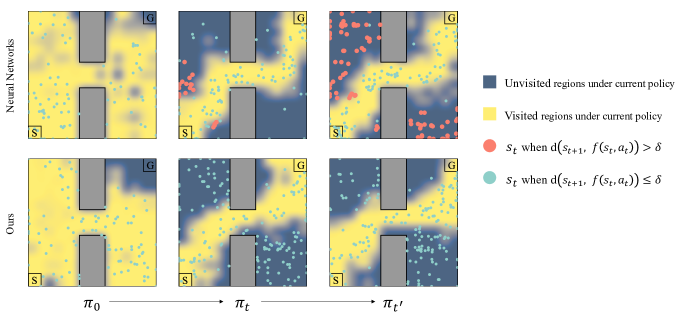
Figure 1: This Gridworld environment requires the agent to navigate from the start position (“S”) to the goal location (“G”) with shortest path. The tabular Q-learning agent starts from a random policy $\pi_{0}$ and improves to get better policies $\pi_{t}\cdots\pi_{t^{\prime}}$, leading to narrower state visitation towards the optimal trajectories (the yellow regions). Due to such distributional shift, the NN-based model (top) may forget recently under-visited regions, even though it has explored there before. The red circles indicate erroneous predictions where the Euclidean distance between the ground truth next state and the prediction is greater than a threshold ($\delta=0.05$). In contrast, our method (bottom) learns online, and at each step incrementally computes the optimal solution over all accumulated data, thus is resilient to forgetting.

2 Preliminaries

In this section, we first recap the protocol of online learning and introduce the Follow-The-Leader strategy. Then we revisit Dyna, a classic MBRL architecture, where we apply our method to learn world models online.

2.1 Online learning

Online learning refers to a learning paradigm where the learner needs to make a sequence of accurate predictions given knowledge about the correct answers for all prior questions (Shalev-Shwartz et al., 2012). Formally, at round $t$, the online learner is given a question ${\mathbf{x}}_{t}\in\mathcal{X}$ and asked to provide an answer to it, which we denote as $h_{t}({\mathbf{x}}_{t})$, letting $h_{t}\in\mathcal{H}:\mathcal{X}\rightarrow\mathcal{Y}$ be a model in the hypothesis class built by the learner. After predicting the answer, the learner will be revealed the ground truth ${\mathbf{y}}_{t}\in\mathcal{Y}$ and suffers a loss $\ell(h_{t}({\mathbf{x}}_{t}),{\mathbf{y}}_{t})$. The learner’s goal is to adjust its model to achieve the lowest possible regret relative to $\mathcal{H}$ defined as $\text{Regret}_{T}(\mathcal{H})=\max_{h^{*}\in\mathcal{H}}\left(\sum_{t=1}^{T}\ell(h_{t}({\mathbf{x}}_{t}),{\mathbf{y}}_{t})-\sum_{t=1}^{T}\ell(h^{*}({\mathbf{x}}_{t}),{\mathbf{y}}_{t})\right)$. When the input is a convex set $\mathcal{S}$, the prediction is a vector ${\mathbf{w}}_{t}\in\mathcal{S}$, and the loss $\ell({\mathbf{w}}_{t},{\mathbf{y}}_{t})$ is convex, the problem is cast as online convex optimization. Absorbing the target into the loss, $\ell_{t}({\mathbf{w}}_{t})=\ell({\mathbf{w}}_{t},{\mathbf{y}}_{t})$, the regret with respect to a competing hypothesis (a vector ${\mathbf{u}}$) is then defined as $\text{Regret}_{T}({\mathbf{u}})=\sum_{t=1}^{T}\ell_{t}({\mathbf{w}}_{t})-\sum_{t=1}^{T}\ell_{t}({\mathbf{u}})$. One intuitive strategy is for the learner to predict a vector ${\mathbf{w}}_{t}$ at any online round such that it achieves minimal loss over all past rounds. This strategy is usually referred to as Follow-The-Leader (FTL):

$$\forall t,\ {\mathbf{w}}_{t}=\operatorname*{arg\,min}_{{\mathbf{w}}\in\mathcal{S}}\sum_{i=1}^{t-1}\ell_{i}({\mathbf{w}}).$$ (1)

2.2 Model-based reinforcement learning with Dyna

Reinforcement learning problems are usually formulated with the standard Markov Decision Process (MDP) $\mathcal{M}=\{\mathcal{S},\mathcal{A},P,R,\gamma,P_{0}\}$, where $\mathcal{S}$ and $\mathcal{A}$ denote the state and action spaces, $P({\mathbf{s}}^{\prime}|{\mathbf{s}},{\mathbf{a}})$ the Markovian transition dynamics, $R({\mathbf{s}},{\mathbf{a}},{\mathbf{s}}^{\prime})$ the reward function, $\gamma\in(0,1)$ the discount factor, and $P_{0}$ the initial state distribution. The goal of RL is to learn the optimal policy that maximizes the discounted cumulative reward: $\pi^{*}=\operatorname*{arg\,max}_{\pi}\mathbb{E}_{\pi,P}\left[\sum_{t=0}^{\infty}\gamma^{t}R\left({\mathbf{s}}_{t},{\mathbf{a}}_{t},{\mathbf{s}}_{t+1}\right)\mid{\mathbf{s}}_{0}={\mathbf{s}}\sim P_{0}\right]$. Model-based RL solves the optimal policy with a learned world model. Existing NN-based MBRL methods (Schrittwieser et al., 2020; Hansen et al., 2022; Hafner et al., 2023) have shown state-of-the-art performance on various domains but rely heavily on techniques to make data more stationary, such as maintaining a large replay buffer or periodically updating the target network. With these components removed, they would fail to work. When they fail, however, it is unclear how much is due to the forgetting in policies, value functions, or world models because all components are entangled and trained end-to-end in these methods. Therefore, we focus on Dyna, which learns a world model (or simply model in RL literature) alongside learning the base agent in a decoupled manner.

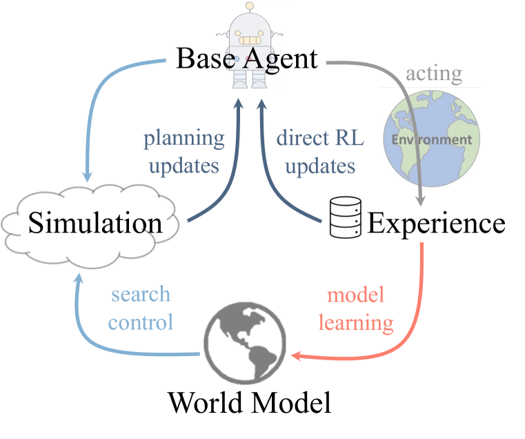
Figure 2: The Dyna architecture.

Figure 2 illustrates the Dyna architecture that we employ in this paper to study online model learning. The base agent will act in the environment and collect environment experiences, which can be used for learning the world model to mimic the environment’s behavior. With such a model learned, the agent then simulate with it to synthesize model experiences for planning updates. Search control defines how the agent queries the model, and some commonly used ones include predecessor (Moore & Atkeson, 1993), on-policy (Janner et al., 2019) and hill-climbing (Pan et al., 2019). Next, we define how to learn and plan with the model.

Model learning. We first formulate how to learn the dynamics model $m({\mathbf{s}}^{\prime}|{\mathbf{s}},{\mathbf{a}})$ with environment experiences. Instead of directly predicting the next state, we model the dynamics as an integrator which estimates the change of the successive states $\hat{{\mathbf{s}}}^{\prime}={\mathbf{s}}+\Delta t\cdot\hat{m}(\Delta{\mathbf{s}}|{\mathbf{s}},{\mathbf{a}})$, where $\Delta t$ is the discrete time step. This technique enables more stable predictions and is widely adopted (Chua et al., 2018; Janner et al., 2019; Yu et al., 2020). The dynamics can either be modeled as a stochastic or a deterministic function, with the former predicting the state-dependent variance besides the mean to capture aleatoric uncertainty in the environment (Chua et al., 2018). We focus on learning a deterministic dynamics model since we are mainly interested in environments without aleatoric uncertainty. As shown in Lutter et al. (2021), deterministic dynamics models can obtain comparable performance with stochastic counterparts. Even when the environment exhibits stochasticity, generating rollouts with fixed variance is also as effective as learned variance (Nagabandi et al., 2020). Therefore, dynamics model learning is a regression problem with the objective

$$\mathbb{E}_{({\mathbf{s}},{\mathbf{a}},{\mathbf{s}}^{\prime})\sim\mathcal{D}_{\text{env}}}\left\|\hat{m}({\mathbf{s}},{\mathbf{a}})-\Delta{\mathbf{s}}\right\|^{2}_{2},$$ (2)

where $\mathcal{D}_{\text{env}}$ is the environment experiences and $\Delta{\mathbf{s}}={\mathbf{s}}^{\prime}-{\mathbf{s}}$. The reward model learning follows a similar regression objective and we will omit it throughout this paper for brevity.

Model planning. In Dyna-style algorithms, the learned model is meant for the agent to interact with, as a substitution of the real environment. When the agent “plans” with the model, it queries the model at $(\tilde{{\mathbf{s}}},\tilde{{\mathbf{a}}})\in\mathcal{S}\times\mathcal{A}$ to synthesize model experiences $\mathcal{D}_{m}=(\tilde{{\mathbf{s}}},\tilde{{\mathbf{a}}},\hat{r},\hat{{\mathbf{s}}}^{\prime})$, which serves as a data source for agent learning. There are various ways to determine how to query the model. For example, the classic Dyna-Q (Sutton, 1990) conducts one-step simulations on state-action pairs uniformly sampled from prior experiences. More recently, MBPO (Janner et al., 2019) generalizes the one-step simulation to short-horizon on-policy rollout branched from observed states and provides theoretical analysis for the monotonic improvement of model-based policy optimization.

3 Learning world models online

The agent-environment interaction generates a temporally correlated data stream ${({\mathbf{s}}_{t},{\mathbf{a}}_{t},r_{t},{\mathbf{s}}_{t+1})}_{t}$. At each time step, the world model observes ${\mathbf{x}}_{t}=[{\mathbf{s}}_{t},{\mathbf{a}}_{t}]\in\mathbb{R}^{S+A}$, predicts the next state and suffers a quadratic loss $\ell_{t}(\hat{m}_{t})=\left\|\hat{m}_{t}({\mathbf{x}}_{t})-{\mathbf{y}}_{t}\right\|^{2}_{2}$, where $S$ and $A$ are the dimensionalities of state and action spaces, ${\mathbf{y}}_{t}=({\mathbf{s}}_{t+1}-{\mathbf{s}}_{t})\in\mathbb{R}^{S}$ is the state difference target. In most model-based RL algorithms built with neural networks, the model learning is conducted in a supervised offline manner, with periodic re-training over the whole dataset (see the objective in Equation 2). Such methods achieve FTL for NNs but are inefficient due to the growing size of the dataset. We develop in this section an online method for learning world models with efficient incremental update on every single environment step.

3.1 Online Follow-The-Leader model learning

Our world model $\hat{m}({\mathbf{x}})=\phi({\mathbf{x}})^{\top}{\mathbf{W}}$ employs a linear function approximation with weights ${\mathbf{W}}\in\mathbb{R}^{D\times S}$ on an expressive and sparse non-linear feature $\phi({\mathbf{x}})\in\mathbb{R}^{D}$. The FTL objective in Equation 1 thus converts to a least squares loss per time step:

$$\forall t,\ {\mathbf{W}}_{t}=\operatorname*{arg\,min}_{{\mathbf{W}}\in\mathbb{R}^{D\times S}}\left\|{\mathbf{\Phi}}_{t-1}{\mathbf{W}}-{\mathbf{Y}}_{t-1}\right\|_{F}^{2},$$ (3)

where ${\mathbf{\Phi}}_{\tau}=[\phi({\mathbf{x}}_{1}),\dots,\phi({\mathbf{x}}_{\tau})]^{\top}\in\mathbb{R}^{\tau\times D}$ denotes non-linear features for observations accumulated until time step $\tau$, ${\mathbf{Y}}_{\tau}=[{\mathbf{y}}_{1},\dots,{\mathbf{y}}_{\tau}]^{\top}\in\mathbb{R}^{\tau\times S}$ is the corresponding targets, and $||\cdot||_{F}$ denotes the Frobenius norm. We can expect our world model with the weights satisfying Equation 3 to have good regret, as the regret of FTL for online linear regression problems with quadratic loss is $\text{Regret}_{T}({\mathbf{W}})=\mathcal{O}(\log T)$ (Shalev-Shwartz et al., 2012; Gaillard et al., 2019). As a consequence, our online learned world model will be immune to forgetting, rendering it suitable for lifelong agents.

In the following sections, we present how to attain a feature representation that is expressive enough for modeling complex transition dynamics (Section 3.2), as well as how its sparsity helps to achieve efficient incremental update (Section 3.3).

3.2 Feature representation

We construct high-dimensional sparse features using random projection followed by soft binning. The input vector ${\mathbf{x}}_{t}\in\mathbb{R}^{S+A}$ is first projected into feature space $\sigma:{\mathbf{x}}\rightarrow{\mathbf{P}}{\mathbf{x}}$, where ${\mathbf{P}}\in\mathbb{R}^{d\times(S+A)}$ is a random projection matrix sampled from a multivariate Gaussian distribution so that the transformation approximately preserves similarity in the original space (Johnson & Lindenstrauss, 1984). Afterwards, each element of $\sigma({\mathbf{x}}_{t})$ is binned in a soft manner by locating its neighboring edges as indices and computing the distances between all edges as values. We denote the binning operation as $b:\mathbb{R}^{d}\rightarrow\mathbb{R}^{D}$, where $D\gg d$. Compared to naive binning which produces binary one-hot vectors and loses precision, ours has greater discriminative power by generating multi-hot real-valued representations.

We provide the following example to illustrate. Assume we are binning $\sigma_{1}({\mathbf{x}}_{t})=1.7$ into a $1$-d grid with edges $[0,1,2,3]$. The naive binning would generate a vector $[0,1,0]$ to indicate the value falls into the central bin. In comparison, the soft binning first locates the neighbors $1$ and $2$ as indices, and computes distances to the neighbors as values, thus forming a vector $[0,0.7,0.3,0]$. Our soft binning can discriminate two inputs falling inside the same bin, such as $\sigma_{1}({\mathbf{x}}_{t})=1.7$ and $\sigma_{1}({\mathbf{x}}_{t})=1.2$, while naive binning fails to do so.

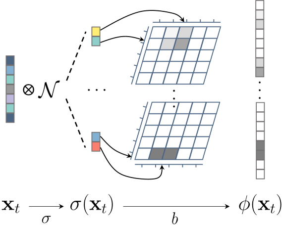
Figure 3: Locality sensitive sparse encoding. $\sigma(\cdot)$ projects input vectors into a random feature space, and $b(\cdot)$ softly bins $\sigma({\mathbf{x}}_{t})$ into multiple $\rho$-dimensional grids, which are flattened and stacked into a high-dimensional sparse encoding $\phi({\mathbf{x}}_{t})$.

Altogether, our feature encoder $\phi=b\circ\sigma$ resembles Locality Sensitive Hashing (LSH) with random projections (Charikar, 2002) but is more expressive thanks to soft binning. We term our feature representation as Locality sensitive sparse encoding, hence Losse. We depict the overall Losse process in Figure 3.

We note that the raw output of $b$ can be multi-dimensional before flattening (e.g. $2$-dimensional in Figure 3), and we use $\rho$ to denote its dimensionality. A $\rho$-dimensional grid has $\lambda$ evenly spaced bins along each axis, thus producing a highly sparse feature vector of length $\lambda^{\rho}$ per grid. Finally, we can stack $\kappa$ grids with different random projection directions to get diverse features. Losse has guaranteed sparsity as stated in Remark 3.1.

Remark 3.1 (Sparsity guarantee of Losse).

For any $\rho,\lambda,\kappa\in\mathcal{Z}_{>0}$, and any input vector ${\mathbf{x}}$, $\phi({\mathbf{x}})$ outputs a vector whose number of nonzero entries $\|\phi({\mathbf{x}})\|_{0}$ satisfies $\|\phi({\mathbf{x}})\|_{0}\leq\kappa 2^{\rho}$, and the proportion of nonzero entries in $\phi({\mathbf{x}})$ is at most $\left(\frac{2}{\lambda}\right)^{\rho}$.

To give a concrete example, if we set $\rho=3$ and $\lambda=10$, then $\|\phi({\mathbf{x}})\|_{0}$ is at most $8\kappa$ while the dimension of $\phi({\mathbf{x}})$ can be as high as $1000\kappa$. The high-dimensional feature brings us more fitting capacity, and the bounded sparsity allows us to do efficient model update with constant overhead, as we will show in the following section.

3.3 Efficient sparse incremental update

A no-regret world model after $t$ steps of interaction can be updated online by computing the weights ${\mathbf{W}}_{t+1}$ as in Equation 3, which can be solved in closed form using the normal equation: ${\mathbf{W}}_{t+1}={\mathbf{A}}_{t}^{-1}{\mathbf{B}}_{t}$, where ${\mathbf{A}}_{t}={\mathbf{\Phi}}_{t}^{\top}{\mathbf{\Phi}}_{t}$ and ${\mathbf{B}}_{t}={\mathbf{\Phi}}_{t}^{\top}{\mathbf{Y}}_{t}$ are two memory matrices. Hence, we obtain a simple algorithm (Algorithm 1) to learn the model online at every time step. Algorithm 1 Online model learning 1:$t=0,{\mathbf{A}}_{0}\in\mathbb{R}^{D\times D}=\textbf{0},{\mathbf{B}}_{0}\in\mathbb{R}^{D\times S}=\textbf{0}$ 2:while True do 3:     $t\leftarrow t+1$ 4:     ${\mathbf{A}}_{t}\leftarrow{\mathbf{A}}_{t-1}+{\phi({\mathbf{x}}_{t})}{\phi({\mathbf{x}}_{t})}^{\top}$ 5:     ${\mathbf{B}}_{t}\leftarrow{\mathbf{B}}_{t-1}+{\phi({\mathbf{x}}_{t})}{\mathbf{y}}_{t}^{\top}$ 6:     ${\mathbf{W}}_{t+1}\leftarrow{\mathbf{A}}_{t}^{-1}{\mathbf{B}}_{t}$ 7:end while Algorithm 2 Sparse online model learning 1:$t=0,{\mathbf{A}}_{0}\in\mathbb{R}^{D\times D}=\textbf{0},{\mathbf{B}}_{0}\in\mathbb{R}^{D\times S}=\textbf{0}$ 2:while True do 3:     $t\leftarrow t+1$ 4:     $s\leftarrow\texttt{nonzero\_index}(\phi({\mathbf{x}}_{t}))$ 5:     ${\mathbf{A}}_{t,{\color[rgb]{0.6,0,0.4}ss}}\leftarrow{\mathbf{A}}_{t-1,{\color[rgb]{0.6,0,0.4}ss}}+\phi_{\color[rgb]{0.6,0,0.4}s}({\mathbf{x}}_{t})\phi_{\color[rgb]{0.6,0,0.4}s}({\mathbf{x}}_{t})^{\top}$ 6:     ${\mathbf{B}}_{t,{\color[rgb]{0.6,0,0.4}s}}\leftarrow{\mathbf{B}}_{t-1,{\color[rgb]{0.6,0,0.4}s}}+\phi_{\color[rgb]{0.6,0,0.4}s}({\mathbf{x}}_{t}){\mathbf{y}}_{t}^{\top}$ 7:     ${\mathbf{W}}_{t+1,{\color[rgb]{0.6,0,0.4}s}}\leftarrow{\mathbf{A}}_{t,{\color[rgb]{0.6,0,0.4}ss}}^{-1}({\color[rgb]{0.6,0,0.4}{\mathbf{B}}_{t,s}-{\mathbf{A}}_{t,s{\overline{s}}}{\mathbf{W}}_{t,{\overline{s}}}})$ 8:end while

Updating the memory matrices ${\mathbf{A}}_{t},{\mathbf{B}}_{t}$ is relatively cheap, but computing weights (line $6$ of Algorithm 1) involves matrix inversion, which is computationally expensive. Though ${\mathbf{W}}_{t+1}$ can be recursively updated using Sherman-Morrison formula (Sherman & Morrison, 1950) as done in Least-Squares TD (Bradtke & Barto, 1996), when the feature becomes very high-dimensional to gain expressiveness, it is still inefficient and may no longer be practical.

Fortunately, the incremental updates ${\phi({\mathbf{x}}_{t})}{\phi({\mathbf{x}}_{t})}^{\top}$ and ${\phi({\mathbf{x}}_{t})}{\mathbf{y}}_{t}^{\top}$ are highly sparse by Losse, so that we can efficiently update a small subset of weights. As shown in Algorithm 2, we first record the indices where the softly binned random features fall into (line $4$), which are used to locate those “activated” entries in the current step and update only a small block of the memory matrices (line $5$-$6$). Most importantly, the inversion for computing the weights can be conducted on a much smaller sub-matrix efficiently while ensuring optimality (line $7$). We next derive how our sparse weight update rule solves Equation 3 in a block-wise manner, which yields an optimal fitting for all data including the current one at each update step.

We first re-index the sparse vector such that it is the concatenation of two vectors $\phi({\mathbf{x}})=[\phi_{\overline{s}}({\mathbf{x}}),\phi_{s}({\mathbf{x}})]$, where all zero entries go to the former and the latter is densely real-valued. We discard the subscript on time step for notational convenience. Intuitively, the new observation ${\mathbf{x}}$ will only update a subset of weights associated with its non-zero feature entries, which we denote as ${\mathbf{W}}_{s}\in\mathbb{R}^{K\times S}$, where $K$ is the dimension of $\phi_{s}({\mathbf{x}})$. Then ${\mathbf{W}}_{\overline{s}}\in\mathbb{R}^{(D-K)\times S}$ is the complement weight matrix. Correspondingly, the accumulative memories ${\mathbf{A}}={\mathbf{\Phi}}^{\top}{\mathbf{\Phi}}$ and ${\mathbf{B}}={\mathbf{\Phi}}^{\top}{\mathbf{Y}}$ can be decomposed as

$${\mathbf{A}}=\begin{pmatrix}{\mathbf{A}}_{{\overline{s}}{\overline{s}}}&{\mathbf{A}}_{{\overline{s}}s}\\ {\mathbf{A}}_{s{\overline{s}}}&{\mathbf{A}}_{ss}\end{pmatrix},\quad{\mathbf{B}}=\begin{pmatrix}{\mathbf{B}}_{{\overline{s}}}\\ {\mathbf{B}}_{s}\end{pmatrix}.$$ (4)

Then the objective in Equation 3 becomes

$$\begin{split}&\operatorname*{arg\,min}_{{\mathbf{W}}}\left(\left\|{\mathbf{\Phi}}{\mathbf{W}}\right\|_{F}^{2}+\left\|{\mathbf{Y}}\right\|_{F}^{2}-2\left<{\mathbf{\Phi}}{\mathbf{W}},{\mathbf{Y}}\right>_{F}\right)\\ \Leftrightarrow&\operatorname*{arg\,min}_{{\mathbf{W}}}\left[\operatorname{Tr}\left(\begin{pmatrix}{\mathbf{W}}_{{\overline{s}}}\\ {\mathbf{W}}_{s}\end{pmatrix}^{\top}\begin{pmatrix}{\mathbf{A}}_{{\overline{s}}{\overline{s}}}&{\mathbf{A}}_{{\overline{s}}s}\\ {\mathbf{A}}_{s{\overline{s}}}&{\mathbf{A}}_{ss}\end{pmatrix}\begin{pmatrix}{\mathbf{W}}_{{\overline{s}}}\\ {\mathbf{W}}_{s}\end{pmatrix}\right)-2\operatorname{Tr}\left(\begin{pmatrix}{\mathbf{W}}_{{\overline{s}}}\\ {\mathbf{W}}_{s}\end{pmatrix}^{\top}\begin{pmatrix}{\mathbf{B}}_{{\overline{s}}}\\ {\mathbf{B}}_{s}\end{pmatrix}\right)\right],\end{split}$$ (5)

where $\left<\cdot,\cdot\right>_{F}$ denotes the Frobenius inner product. Treating ${\mathbf{W}}_{\overline{s}}$ as a constant since it is not affected by current data and optimizing ${\mathbf{W}}_{s}$ only gives

$$\begin{gathered}\operatorname*{arg\,min}_{{\mathbf{W}}_{s}}\left(\cancel{\operatorname{Tr}({\mathbf{W}}_{\overline{s}}^{\top}{\mathbf{A}}_{{\overline{s}}{\overline{s}}}{\mathbf{W}}_{\overline{s}})}+\operatorname{Tr}({\mathbf{W}}_{s}^{\top}{\mathbf{A}}_{ss}{\mathbf{W}}_{s})+2\operatorname{Tr}({\mathbf{W}}_{s}^{\top}{\mathbf{A}}_{s{\overline{s}}}{\mathbf{W}}_{\overline{s}})\right.\\ -\left.\cancel{2\operatorname{Tr}({\mathbf{W}}_{\overline{s}}^{\top}{\mathbf{B}}_{{\overline{s}}})}-2\operatorname{Tr}({\mathbf{W}}_{s}^{\top}{\mathbf{B}}_{s})\right).\end{gathered}$$ (6)

The new objective in Equation 6 is quadratic, so we differentiate with respect to ${\mathbf{W}}_{s}$ and set the derivative to zero to obtain the solution of the sub-matrix

$${\mathbf{W}}_{s}={\mathbf{A}}_{ss}^{-1}({\mathbf{B}}_{s}-{\mathbf{A}}_{s{\overline{s}}}{\mathbf{W}}_{\overline{s}}),$$ (7)

which gives us the sparse update rule in Algorithm 2.

Concluding remark. So far, we have presented an efficient algorithm that learns world models online without forgetting. In our algorithm, linear models are exploited so that we can achieve no-regret online learning with Follow-The-Leader. To enlarge the model capacity, we devise a high-dimensional nonlinear random feature encoding, Losse, turning linear models into universal approximators (Huang et al., 2006). Moreover, the sparsity guarantee of Losse permits efficient updates of the shallow but wide model. We name our method Losse-FTL. We further note that feature sparsity has been utilized to mitigate catastrophic forgetting (McCloskey & Cohen, 1989; French, 1991; Liu et al., 2019; Lan & Mahmood, 2023). Our work differs from them in that not only does sparsity help reduce feature interference, but the incremental closed-form solution also guarantees the optimal fitting of all observed data, thus eliminating forgetting. More discussion on feature sparsity can be found in Appendix A, and the implementation details of Losse-FTL can be found in Appendix D.

4 Empirical results on supervised learning

In this section, we will showcase empirical results to validate the expressiveness of Losse (Section 4.1) and the online learning capability of Losse-FTL (Section 4.2), both in supervised learning settings.

4.1 Comparing feature representations

We compare our locality sensitive sparse encoding with other feature encoding techniques, including Random Fourier Features (Rahimi & Recht, 2007), Random ReLU Features (Sun et al., 2018), and Random Tile Coding, which combines random projection and Tile Coding (Sutton & Barto, 2018). We note that in all these methods including ours, random projections are used to construct high-dimensional features to acquire more representation power. However, they have different properties with regards to the sparsity and feature values, as summarized in Table 1. Losse is designed to be sparse and real-valued. Sparse encoding allows for more efficient incremental update (Algorithm 2), while distance-based real values provide better generalization. Although ReLU also produces sparse features, it does not guarantee the sparsity level, which is dependent on the sign of its outputs.

We test different encoding methods on an image denoising task, where the inputs are MNIST (Deng, 2012) images with Gaussian noise, and the outputs are clean images. The flattened noisy images are first encoded by different methods to produce feature vectors, on which a linear layer is applied to predict the clean images of the same size. We use mini-batch stochastic gradient descent to optimize the weights of the linear layer until convergence. To keep the online update efficiency similar, we keep the same number of non-zero entries for all encoding methods. The mean squared errors on the test set for different patch sizes are reported in Table 1. We observe that Losse achieves the lowest error across all patch sizes, justifying its representational strength over other non-linear feature encoders. When compared with the NN baseline, which is a strong function approximator but not an efficient online learner, linear models with Losse work better when the patch size is $36$ or smaller, suggesting its sufficient capacity for problems with a moderate number of dimensions, such as locomotion or robotics (Todorov et al., 2012; Zhu et al., 2020). See Appendix B.1 for more experimental details.

	Sparse	Real-value	9	16	25	36	49
NN	-	-	0.36	0.35	0.34	0.34	0.33
Fourier	✗	✓	0.32	0.39	0.67	1.00	1.40
ReLU	✓✗	✓	0.35	0.34	0.37	0.39	0.43
Tile Code	✓	✗	0.36	0.39	0.51	0.61	0.73
Losse	✓	✓	0.28	0.29	0.31	0.34	0.40

Table 1: Properties of different encoding methods and their mean squared errors on the image denoising task on different patch sizes. All numbers are scaled by $10^{-1}$.

Figure 4: Mean squared errors on the stream learning task of different correlation levels. Solid lines and shaded areas correspond to the means and stand errors of $30$ runs.

4.2 Online learning with covariate shift

Next, we consider a supervised stream learning setting, where we can precisely control the level of covariate shift in the training data, and test the online learning capability of Losse-FTL against the neural network counterpart. Similar to Pan et al. (2021), we create a synthetic data stream with observations sampled from a non-stationary input distribution. Specifically, the synthetic data is generated according to a Piecewise Random Walk. At each time step, the observation is sampled from a Gaussian $X_{t}\sim\mathcal{N}(S_{t},\beta^{2})$, where $\beta$ is fixed and $S_{t}$ drifts every $\tau$ steps. The drifting follows a Gaussian first order auto-regressive random walk $S_{t+1}=(1-c)S_{t}+Z_{t},\forall t\bmod\tau\equiv 0$, where $c\in(0,1]$ and $Z_{t}\sim\mathcal{N}(0,\sigma^{2})$ with a fixed $\sigma$. For $X_{t}=x_{t}$, the target is defined as $y_{t}=\sin{(2\pi x_{t}^{2})}$.

As proven in Pan et al. (2021), $X_{t}$ can share the same equilibrium distribution but possess different levels of temporal correlation if $\beta,c$, and $\sigma$ are properly chosen. It turns out the three scalars can be uniquely determined by a single parameter $d\in[0,1)$, which we call correlation level. When $d=0$, the generated data recovers i.i.d. property. Given the data stream $\{(x_{t},y_{t})\}_{t\in\mathbb{N}}$, we fit our model online and measure the mean squared error at the end of learning on a holdout test set, which contains independent samples across all $S_{t}$. As a comparison, we use neural networks to fit online as well as in batch and plot the errors under different correlation levels in Figure 4. The results show that our method outperforms neural networks in two aspects. First, when the data is i.i.d. ($d=0$), Losse-FTL achieves a much lower error than NN-online. This indicates neural networks with gradient descent have low sample efficiency, even on stationary data. Training NNs using batch samples alleviates the issue and reaches a similar performance to ours. Second, our model consistently attains very low error across all correlation levels, showing its capacity of non-forgetting online learning. In contrast, neural networks learned with both batch and online updates incur increasingly high errors when $d$ is large, indicating catastrophic forgetting in the presence of data nonstationarity. More experimental details can be found in Appendix B.2.

5 Empirical results on reinforcement learning

In this section, we will demonstrate that world models built with Losse-FTL can be accurately learned online, outperforming several NN-based world model baselines and improving the data efficiency of RL agents. We first introduce the settings and baselines in Section 5.1, and then present our results in Section 5.2.

5.1 Settings and baselines

We employ the Dyna MBRL architecture and restrict our study to the model learning part, keeping the base agent’s value (and policy) learning untouched. We compare Losse-FTL world models learned online with their NN-based counterparts, using the same model-free base agent. We introduce the baselines below. The algorithm and more experimental details can be found in Appendix C.

Model-free. The model-free base agent used in Dyna. We use two strong off-policy agents: DQN (Mnih et al., 2015) for discrete action space and SAC (Haarnoja et al., 2018) for continuous action space. All other settings below are MBRL coupled with either DQN or SAC.

Full-replay. We use neural networks to build the world model and train the NNs over all collected data till convergence. Before the training loop starts, the data is split into train and holdout sets with a ratio of $4$:$1$. The loss on the holdout set is measured after each epoch. We stop training if the loss does not improve over $5$ consecutive epochs. The NNs are trained continuously without resetting the weights (Nagabandi et al., 2020). This is the closest setting to FTL for NNs, but with growing computational cost as the data accumulates.

Online. We train NN-based world models in a stream learning fashion, where only a mini-batch of $256$ transitions is kept for training. However, we still update the model for $250$ gradient descent steps on each mini-batch, unlike our method which only needs a single pass of the interaction trajectory.

SI. This is similar to Online, but the NN is trained with Synaptic Intelligence (SI) (Zenke et al., 2017), a regularization-based continual learning (CL) method to overcome catastrophic forgetting. However, there is no explicit task boundary defined in the RL process, thus we adapt SI to treat each training sample as a new task.

Coreset. This refers to rehearsal-based CL methods (Lopez-Paz & Ranzato, 2017; Chaudhry et al., 2019) that keep an important subset of experiences for replay. There are different ways to decide whether to keep or remove a data point. We use Reservoir sampling (Vitter, 1985), which uniformly samples a subset of items from a stream of unknown length. Similar to Full-replay, data split and early stopping strategies are adopted for each training epoch.

Figure 5: Learning curves showing normalized episode return. We compare our method with five baselines on (top) discrete control and (bottom) continuous control benchmarks. Solid curves depict the means of multiple runs with different random seeds, while shaded areas represent standard errors.

5.2 Results

The learning curves are presented in Figure 5, where we compare Losse-FTL with aforementioned baselines on $6$ environments. We first revisit the discrete control Gridworld environment, which is used for illustration in Figure 1. This environment is a variant of the one introduced by Peng & Williams (1993) to test Dyna-style planning. The agent is required to navigate from the starting location to the goal position without being blocked by the barrier. A small offset is added on each step to make the state space continuous. In such navigation tasks, intuitively, the world model needs to learn from extremely nonstationary data. When the agent evolves from randomly behaving to nearly optimal, its state visitation changes dramatically, making all NN-based world models completely fail to learn due to catastrophic forgetting, unless experiences are fully replayed (see the first plot in Figure 5). The poorly learned models are unable to provide useful planning, leading to almost zero performance. In contrast, a world model based on Losse-FTL can be learned accurately and improves the data efficiency over Model-free.

In the other two general discrete control tasks, Mountain Car and Acrobot, the data nonstationarity still exists but may be less severe than that in navigation tasks. The results show that Losse-FTL consistently outperforms all baselines and brings sample efficiency improvement.

For continuous control tasks from Gym Mujoco (Todorov et al., 2012), we can observe that Online NN fails to capture the dynamics for all environments, resulting in even worse performance than the Model-free baseline. While SI and Coreset can help reduce forgetting to some extent, their performances vary across tasks and are inferior to Full-replay in all cases. Losse-FTL, however, achieves on-par or even better performance than Full-replay, which is a strong baseline that continuously trains a deep neural network on all collected data until convergence to pursue FTL. These positive results verify the strength of Losse-FTL for building an online world model.

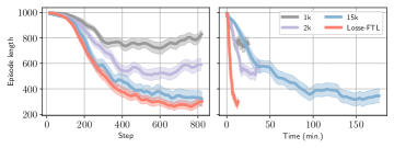
Figure 6: (Left) Sample and (Right) wall-clock efficiency comparison between world models learned with Losse-FTL and Coreset of different replay sizes.

Model update efficiency. Among continual learning methods with neural networks, rehearsal-based ones are closer to the FTL objective and usually demonstrate strong performance (Chaudhry et al., 2019; Boschini et al., 2022). It seems that Coreset can offer a good balance between computation cost and non-forgetting performance with a properly set buffer size. We hence ablate Coreset with different replay sizes and compare their performance with Losse-FTL. Figure 6 shows both the sample efficiency and wall-clock efficiency on the Gridworld environment. Coreset with a small replay size leads to poor asymptotic performance while being relatively more efficient. Increasing the replay size indeed contributes to better results at the cost of more computation. In comparison, Losse-FTL updates the model purely online without any replay buffer and achieves the best performance with the best wall-clock efficiency.

6 Limitation and future work

Currently, we have not validated our method on problems with very high-dimensional state space such as Humanoid, or tasks with image observations. They are expected to be challenging for linear models to directly work on. Extending Losse-FTL to handle such large-scale problems, perhaps using pre-trained models to obtain compact sparse encoding, is a potential avenue for future work.

7 Conclusion

In this work, we investigate the problem of online world model learning using Dyna. We first demonstrate that NN-based world models suffer from catastrophic forgetting when used for MBRL because the data collected in the RL process is innately nonstationary. As a result, re-training over all previous data is adopted by common MBRL methods, which is of low efficiency. Through the lens of online learning, we uncover the implicit connection between NN re-training and FTL, which allows us to formulate online model learning with linear regressors to achieve incremental update. We devise locality sensitive sparse encoding (Losse), a high-dimensional non-linear random feature generator that can be coupled with a linear layer to produce models with greater capacities. We provide a sparsity guarantee for Losse, controlled by two parameters, $\rho$ and $\lambda$, which can be adjusted to develop an efficient sparse update algorithm. We test our method in both supervised learning and MBRL settings, with the presence of data nonstationarity. The positive results verify that Losse-FTL is capable of learning accurate world models online, which enhances both the sample and computation efficiency of reinforcement learning.

Appendix A On feature sparsity

Feature sparsity has been pursued to reduce forgetting dating back to McCloskey & Cohen (1989); French (1991). The core idea is that catastrophic forgetting occurs due to the overlap of distributed representations in NNs, hence it can be reduced by reducing the overlap. Sparse features are local features with less overlap, so they should alleviate the forgetting issue. Recent works have demonstrated positive results by enforcing sparse hidden features in NNs either by regularization (Liu et al., 2019; Hernandez-Garcia & Sutton, 2019) or by deterministic activation functions (Pan et al., 2021; Lan & Mahmood, 2023). However, we emphasize that, in our work, non-forgetting is ensured by FTL and the high-dimensional sparse encoding is mainly for representational capacity and computational efficiency, though it also reduces feature interference as a byproduct.

We first conduct theoretical analysis similar to Lan & Mahmood (2023) to understand how sparsity contributes to non-forgetting, then present empirical results to show sparsity alone is not sufficient to guarantee non-forgetting.

Assume we are regressing a scalar target given an input vector using squared loss: $\ell(f,{\mathbf{x}},y)=(f_{\mathbf{w}}({\mathbf{x}})-y)^{2}$, where $f$ is our predictor with parameters ${\mathbf{w}}$. When a new data sample $\{{\mathbf{x}}_{t},y_{t}\}$ arrives, we want to adjust the parameters ${\mathbf{w}}$ to minimize $\ell(f,{\mathbf{x}}_{t},y_{t})$ with gradient descent:

$${\mathbf{w}}^{\prime}-{\mathbf{w}}=\Delta{\mathbf{w}}=-\alpha\nabla_{\mathbf{w}}\ell(f,{\mathbf{x}}_{t},y_{t})$$ (8)

The change of the parameters will lead to the change of the predictor’s output, and by the first-order Taylor expansion:

$$\begin{split}f_{{\mathbf{w}}^{\prime}}({\mathbf{x}})-f_{\mathbf{w}}({\mathbf{x}})&\approx\nabla_{\mathbf{w}}f_{\mathbf{w}}({\mathbf{x}})\left({\mathbf{w}}^{\prime}-{\mathbf{w}}\right)\\ &=-\alpha\nabla_{\mathbf{w}}f_{\mathbf{w}}({\mathbf{x}}){\color[rgb]{0,0,1}\nabla_{\mathbf{w}}\ell(f,{\mathbf{x}}_{t},y_{t})}\\ &=-\alpha{\color[rgb]{0,0,1}\nabla_{f}\ell(f,{\mathbf{x}}_{t},y_{t})}\langle\nabla_{\mathbf{w}}f_{\mathbf{w}}({\mathbf{x}}),{\color[rgb]{0,0,1}\nabla_{\mathbf{w}}f_{\mathbf{w}}({\mathbf{x}}_{t})}\rangle\end{split}$$ (9)

We assume non-zero loss so $\nabla_{f}\ell(f,{\mathbf{x}}_{t},{\mathbf{y}}_{t})\neq 0$ and analyze $\langle\nabla_{\mathbf{w}}f_{\mathbf{w}}({\mathbf{x}}),\nabla_{\mathbf{w}}f_{\mathbf{w}}({\mathbf{x}}_{t})\rangle$. For linear models as in our case, $f_{\mathbf{w}}({\mathbf{x}})={\mathbf{w}}^{\top}\phi({\mathbf{x}})$, thus $\langle\nabla_{\mathbf{w}}f_{\mathbf{w}}({\mathbf{x}}),\nabla_{\mathbf{w}}f_{\mathbf{w}}({\mathbf{x}}_{t})\rangle=\langle\phi({\mathbf{x}}),\phi({\mathbf{x}}_{t})\rangle$. Then we could investigate the following question: after we adjust the parameters (Equation 8) based on the new sample, what’s the output difference (Equation 9) at any ${\mathbf{x}}$ for ${\mathbf{x}}$ that is similar or dissimilar to ${\mathbf{x}}_{t}$?

1. For ${\mathbf{x}}$ similar to ${\mathbf{x}}_{t}$, we expect $\langle\phi({\mathbf{x}}),\phi({\mathbf{x}}_{t})\rangle\neq 0$ to yield improvement and generalization. This will hold since a proper feature encoder $\phi(\cdot)$ should approximately preserve the similarity in the original space.

2. For ${\mathbf{x}}$ dissimilar to ${\mathbf{x}}_{t}$, we hope $\langle\phi({\mathbf{x}}),\phi({\mathbf{x}}_{t})\rangle\approx 0$ to reduce interference (therefore less forgetting). The claim is that if $\phi(\cdot)$ produces sparse features, it is highly likely that the inner product is approximately zero, hence meeting our expectation.

However, we argue that feature sparsity is not sufficient to mitigate forgetting, because the probability that there is no single overlap between representations is low even if the feature is sparse. In Figure 7, we show the mean squared errors for the piecewise random walk stream learning task introduced in Section 4.2. We use our Losse representation with different sparsity levels as features and compare our sparse FTL update with gradient descent update. We can observe that the gradient descent update relying on feature sparsity still suffers from catastrophic forgetting until $\lambda=30$, which corresponds to a $9000$-dimensional feature with $40$ nonzero entries — an extremely high sparsity level. Nevertheless, increasing sparsity indeed helps sparse features to reduce interference when using gradient descent (comparing the absolute values of MSEs across different $\lambda$). In contrast, Losse-FTL ensures non-forgetting incrementally by finding the optimal fitting for all experienced samples, even with the presence of feature overlap. Notably, when Losse gets more sparse, we can observe the error for Losse-FTL decreases, verifying our design that the high dimensional sparse feature brings more fitting capacity while maintaining the same computational cost with our sparse update.

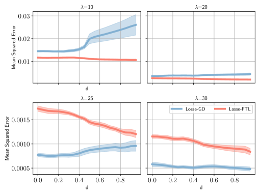
Figure 7: Mean squared errors on piecewise random walk stream learning. The results compare the FTL update to the gradient descent update using Losse features with different sparsity levels. Note that gradient descent (GD) update uses a mini-batch of $50$ samples for each update, resulting in lower errors than FTL’s when the feature dimension gets higher.

Appendix B Supervised learning details

In this section, we provide more details regarding the supervised learning experiments on image denoising (Appendix B.1) and piecewise random walk (Appendix B.2).

B.1 Image denoising

We add pixel-wise Gaussian noise with $\mu=0,\sigma=0.3$ to normalized images from the MNIST dataset (Deng, 2012), and create train and test splits with ratio $9:1$. To test the feature representation on different difficulties, we crop patches from the center with different sizes, ranging from $2\times 2$ to $7\times 7$. Figure 8 shows some sample pairs.

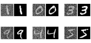
Figure 8: Sample pairs for the image denoising task.

For different feature encoding methods compared in Section 4.1, we limit the number of non-zero feature entries up to $80$ for fair comparison. This means $2$-d binning with $20$ grids for Losse-FTL. The number of bins affects the performance slightly, due to different granularity for generalization. Hence we sweep it over $\{5,6,7,8,9\}$. We observe that the scale of the standard deviation of the Gaussian random projection matrix affects the final performance significantly for random ReLU and random Frouier features, so we select the best one from a sweep over $\{0.1,0.3,0.5,1,5,10\}$. The linear layer is optimized using Adam (Kingma & Ba, 2015) with a learning rate $0.0001$. We repeated experiments for all settings for $5$ times and report the mean scores.

B.2 Piecewise random walk

Recall that observations in the process are sampled from a Gaussian $X_{t}\sim\mathcal{N}(S_{t},\beta^{2})$ with $\{S_{t}\}_{t\in\mathbb{N}}$ being a Gaussian first order auto-regressive random walk $S_{t+1}=(1-c)S_{t}+Z_{t}$, where $c\in(0,1]$ and $Z_{t}\sim\mathcal{N}\left(0,\sigma^{2}\right)$. The equilibrium distribution of $\{X_{t}\}_{t\in\mathbb{N}}$ is also a Gaussian with $\mathbb{E}[X_{t}]=0$ and variance $\xi^{2}=\beta^{2}+\frac{\sigma^{2}}{2c-c^{2}}$. We can use a single parameter $d\in[0,1)$, which we call correlation level, to control the variance:

$$c =1-\sqrt{1-d},$$

$$\sigma^{2} =d^{2}\left(\frac{B}{2}\right)^{2},$$

$$\beta^{2} =(1-d)\left(\frac{B}{2}\right)^{2},$$

where $B$ gives a high probability bound. See Pan et al. (2021) for detailed derivation.

We visualize sampling trajectories of $X_{t}$ for $B=1$ $d\in[0,1)$ in Figure 9.

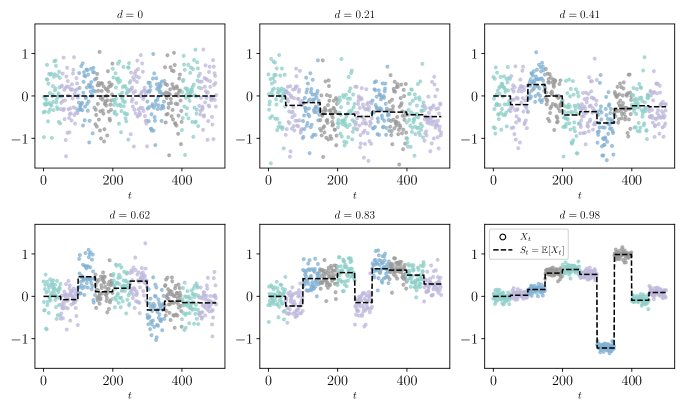
Figure 9: Visualization of piecewise random walk sampling trajectories with different correlation levels $d$.

For neural networks trained in Section 4.2, we use $2$-layer MLP with $50$ hidden units. For NN-Batch, we take $50$ samples from each $X_{t}$ and use mini-batch gradient descent to update the weights. Adam optimizer is used with the best learning rate swept from $\{5\times 10^{-6},1\times 10^{-5},5\times 10^{-5},\dots,1\times 10^{-2}\}$. For Losse-FTL, we use $2$-d binning with $10$ bins for each grid and use $10$ grids to construct the final feature. We run all experiments for $50$ independent seeds and report the means and standard errors.

Appendix C Reinforcement learning details

Learning algorithm. We present the detailed Dyna-style algorithm based on Losse-FTL  in Algorithm 3, where the world models are learned online. For NN-based settings, line $4$ of Algorithm 3 is replaced by training a neural network (optionally with replay buffer or other continual learning techniques).

Algorithm 3 Dyna MBRL with Losse-FTL

1:environment $\mathcal{M}$, agent $\pi$, world model $\hat{f}$, state search control $c$, model unroll length $k$, model experiences $\mathcal{D}_{m}$

2:for epoch $\in\{1,\dots,E\}$ do

3:     for interaction $\in\{1,\dots,K\}$ do

4:         ${\mathbf{s}},{\mathbf{a}},{\mathbf{s}}^{\prime},r\leftarrow\texttt{rollout}(\mathcal{M},\pi)$

5:         Update $\hat{f}$ with $({\mathbf{s}},{\mathbf{a}},{\mathbf{s}}^{\prime},r)$ (Algorithm 2) $\triangleright$ incremental model updates

6:     end for

7:     for planning $\in\{1,\dots,N\}$ do

8:         $\tilde{{\mathbf{s}}}\leftarrow c$ $\triangleright$ uniform state sampling

9:         $\tilde{{\mathbf{a}}},\hat{{\mathbf{s}}}^{\prime},\hat{r}\leftarrow\texttt{ModelUnroll}(\hat{f},\tilde{{\mathbf{s}}},\pi,k)$ $\triangleright$ short-horizon on-policy unroll

10:         $\mathcal{D}_{m}\leftarrow(\tilde{{\mathbf{s}}},\tilde{{\mathbf{a}}},\hat{{\mathbf{s}}}^{\prime},\hat{r})$

11:     end for

12:     for learning $\in\{1,\dots,G\}$ do

13:         Update DQN or SAC on a batch of model data $\mathcal{B}\sim\mathcal{D}_{m}$

14:     end for

15:end for

Settings for discrete control tasks. We use $\kappa=30,\rho=2$, and $\lambda=10$ for Losse-FTL, and $3$-layer MLPs with $32$ hidden units for neural networks. For Coreset we maintain a buffer with size $100$, and for SI we use the best $\xi$ and $c$ from a grid search. The DQN parameters are updated using real data with an interval of $4$ interactions. In MBRL, $16$ planning steps are conducted after each real data update. Both real data updates and planning updates use a mini batch of $32$. The learning rate of DQN is swept from $\{1\times 10^{-2},3\times 10^{-3},1\times 10^{-3},\dots,1\times 10^{-5}\}$ for all configurations. All world models are updated every $25$ environment steps to accelerate experiments. We run all experiments for $30$ independent seeds and report the means and standard errors.

Settings for continuous control tasks. We use $\kappa=300,\rho=2$, and $\lambda=10$ for Losse-FTL, and $4$-layer MLPs with $400$ hidden units for neural networks following Janner et al. (2019). Our implementation follows closely the official codebase of MBPO (Janner et al., 2019), and also adopts the same hyper-parameters for both MBPO and SAC. The replay size of Coreset is $5000$, and the hyper-parameters for SI are chosen from a grid search. All world models are updated every $250$ environment steps to accelerate experiments. We run all experiments for $5$ independent seeds and report the means and standard errors.

Appendix D Implementation details

We provide more implementation details of Losse-FTL in this section. Referring to Figure 3, the input ${\mathbf{x}}_{t}$ is first pre-processed to be bounded between $[-3,3]$, and then projected with a matrix containing values sampled from an isotropic Gaussian with $\mathbf{\mu}=\mathbf{0}$ and $\mathbf{\Sigma}=\frac{1}{c}\mathbf{I}$, where $c$ is the fan-in dimension, i.e., $S+A$. This ensures the projected values $\sigma({\mathbf{x}}_{t})$ are bounded with high probability and facilitates a more even bin utilization. In computing the sparse update at line 7 of Algorithm 2, we use $({\mathbf{A}}_{t,ss}+\varepsilon{\mathbf{I}})^{-1}$ for some small $\varepsilon>0$ to ensure its invertibility. We provide Jax-based Python codes in Figure 10.

⬇

import math

from typing import NamedTuple, Tuple

import chex

import jax

import jax.numpy as jnp

import numpy as np

class LosseParams(NamedTuple):

count: jax.Array

projection: jax.Array

xtx: jax.Array

xty: jax.Array

w: jax.Array

def _to_1d_index(indices, offsets, n_feat, bin_dim, n_bins):

”””Compute the flattened index into the weight matrix.”””

n_grids_per_lsh = (n_bins + 1) ** bin_dim

indices = jnp.reshape(indices, (-1, bin_dim, n_feat))

offsets = jnp.reshape(offsets, (-1, bin_dim, n_feat))

indices = jnp.stack([indices, indices + 1], axis=-1) # [-1, bin_dim, n_feat, 2]

values = jnp.stack([1.0 - offsets, offsets], axis=-1) # [-1, bin_dim, n_feat, 2]

multiplier = jnp.power(n_bins + 1, jnp.arange(bin_dim - 1, -1, -1))

indices *= multiplier[:, None, None]

# shape = (-1, n_feat, ) + (2,) * bin_dim

shape_suffix = [tuple(*p) for p in np.split(np.eye(bin_dim, dtype=np.int32) + 1, bin_dim)]

indices = sum(jnp.reshape(indices[:, i], (-1, n_feat, *suffix)) for i, suffix in enumerate(shape_suffix))

values = math.prod(jnp.reshape(values[:, i], (-1, n_feat, *suffix)) for i, suffix in enumerate(shape_suffix))

# both indices and values has the shape (-1, n_feat, *(2,)*bin_dim) now.

indices += jnp.expand_dims(

n_grids_per_lsh * jnp.arange(n_feat), axis=tuple(range(-bin_dim, 1, 1))

) # expand 1 dim in the front and bin_dim in the back.

indices = jnp.reshape(indices, (-1, n_feat * 2**bin_dim))

values = jnp.reshape(values, (-1, n_feat * 2**bin_dim))

return indices, values

class Losse:

”””Linear regressor with LOcality Sensitive Sparse Encoding (Losse).

We update the linear weights online sparsely following Algorithm.2 in the paper, i.e., computing the incremental closed-form solution based on newly incoming data points.

”””

def __init__(

self,

inout_dims: Tuple[int, int],

num_features: int,

num_bins: int,

bin_dim: int,

eps: float,

) -> None:

self.num_features = num_features

self.num_bins = num_bins

self.bin_dim = bin_dim

self.inout_dims = inout_dims

self.eps = eps

n_edges = num_bins + 1

n_grids_per_lsh = (n_edges + 1) ** bin_dim

self.d = n_grids_per_lsh * num_features

def init(self, rng: jax.random.PRNGKey) -> LosseParams:

input_dim = self.inout_dims[0]

output_dim = self.inout_dims[1]

std = 1 / jnp.sqrt(input_dim)

projection = std * jax.random.truncated_normal(

rng,

-2,

2,

(input_dim, self.num_features * self.bin_dim),

)

return LosseParams(

count=jnp.array(0, dtype=jnp.int64),

projection=projection,

xtx=jnp.zeros((self.d * self.d,), dtype=projection.dtype),

xty=jnp.zeros((self.d, output_dim), dtype=projection.dtype),

w=jnp.zeros((self.d, output_dim), dtype=projection.dtype),

)

def update(

self,

params: LosseParams,

x: jax.Array,

y: jax.Array,

) -> LosseParams:

chex.assert_tree_shape_prefix((x, y), (1,)) # assert non-batched

indices, values = self._indices_and_values(params.projection, x)

params = self._update_memory(params, indices, values, y)

params = self._update_w(params, indices)

return params

def predict(self, params: LosseParams, x: jax.Array):

indices, values = self._indices_and_values(params.projection, x)

output = params.w[indices] * values[…, None]

return output.sum(1)

def _indices_and_values(

self,

projection: jax.Array,

x: jax.Array,

):

h = jnp.matmul(x, projection)

h = jax.nn.sigmoid(h)

h = jnp.clip(h, 0, 1) * self.num_bins

indices = jnp.floor(h).astype(jnp.int32)

offsets = h - indices

indices, values = _to_1d_index(

indices,

offsets,

self.num_features,

self.bin_dim,

self.num_bins,

)

return indices, values

def _update_memory(

self,

params: LosseParams,

indices: jax.Array,

values: jax.Array,

y: jax.Array,

) -> LosseParams:

chex.assert_equal_shape_prefix((indices, values, y), prefix_len=1)

xtx_indices = (indices * self.d)[:, :, None] + indices[:, None, :]

xtx_indices = xtx_indices.flatten()

xty_indices = indices.flatten()

xtx_updates = values[:, :, None] * values[:, None]

xtx_updates = xtx_updates.flatten()

xty_updates = values[:, :, None] * y[:, None, :]

xty_updates = xty_updates.reshape(-1, y.shape[-1])

return params._replace(

xtx=params.xtx.at[xtx_indices].add(xtx_updates),

xty=params.xty.at[xty_indices].add(xty_updates),

count=params.count + y.shape[0],

)

def _update_w(

self,

params: LosseParams,

indices: jax.Array,

) -> LosseParams:

indices = indices.flatten()

sub_indices = (indices * self.d)[:, None] + indices[None, :]

sub_xtx = jnp.reshape(params.xtx[sub_indices], [indices.shape[0]] * 2)

sub_xty = params.xty[indices]

a = sub_xtx

sub_xtxw = jnp.matmul(

jnp.reshape(params.xtx, (self.d, self.d))[indices],

params.w,

)

b = sub_xty - sub_xtxw + jnp.matmul(sub_xtx, params.w[indices])

a_norm = a / params.count + self.eps * jnp.eye(len(a))

b_norm = b / params.count

solution = jnp.linalg.solve(a_norm, b_norm)

return params._replace(w=params.w.at[indices].set(solution))

losse = Losse(

inout_dims=(1, 1),

num_features=50,

num_bins=10,

bin_dim=2,

eps=1e-5,

)

losse.init = jax.jit(losse.init)

losse.update = jax.jit(losse.update, donate_argnums=(0,)) # donate to avoid copy

losse.predict = jax.jit(losse.predict)

Jax-based Python codes for learning an online linear regressor with Losse-FTL.

References

- Boschini et al. (2022) Matteo Boschini, Lorenzo Bonicelli, Pietro Buzzega, Angelo Porrello, and Simone Calderara. Class-incremental continual learning into the extended der-verse. IEEE Transactions on Pattern Analysis and Machine Intelligence, 2022.
- Bradtke & Barto (1996) Steven J Bradtke and Andrew G Barto. Linear least-squares algorithms for temporal difference learning. Machine Learning, 1996.
- Charikar (2002) Moses S Charikar. Similarity estimation techniques from rounding algorithms. In Proceedings of the Thiry-fourth Annual ACM Symposium on Theory of Computing, 2002.
- Chaudhry et al. (2019) Arslan Chaudhry, Marcus Rohrbach, Mohamed Elhoseiny, Thalaiyasingam Ajanthan, P Dokania, P Torr, and M Ranzato. Continual learning with tiny episodic memories. In Workshop on Multi-Task and Lifelong Reinforcement Learning at ICML, 2019.
- Chua et al. (2018) Kurtland Chua, Roberto Calandra, Rowan McAllister, and Sergey Levine. Deep reinforcement learning in a handful of trials using probabilistic dynamics models. Advances in Neural Information Processing Systems, 2018.
- Deng (2012) Li Deng. The mnist database of handwritten digit images for machine learning research. IEEE Signal Processing, 2012.
- Eldan & Shamir (2016) Ronen Eldan and Ohad Shamir. The power of depth for feedforward neural networks. In Conference on Learning Theory, 2016.
- French (1991) Robert M French. Using semi-distributed representations to overcome catastrophic forgetting in connectionist networks. In Proceedings of the 13th Annual Cognitive Science Society Conference, 1991.
- French (1999) Robert M French. Catastrophic forgetting in connectionist networks. Trends in Cognitive Sciences, 1999.
- Gaillard et al. (2019) Pierre Gaillard, Sébastien Gerchinovitz, Malo Huard, and Gilles Stoltz. Uniform regret bounds over for the sequential linear regression problem with the square loss. In Algorithmic Learning Theory, 2019.
- Haarnoja et al. (2018) Tuomas Haarnoja, Aurick Zhou, Pieter Abbeel, and Sergey Levine. Soft actor-critic: Off-policy maximum entropy deep reinforcement learning with a stochastic actor. In International Conference on Machine Learning, 2018.
- Hafner et al. (2023) Danijar Hafner, Jurgis Pasukonis, Jimmy Ba, and Timothy Lillicrap. Mastering diverse domains through world models. arXiv preprint arXiv:2301.04104, 2023.
- Hansen et al. (2022) Nicklas Hansen, Xiaolong Wang, and Hao Su. Temporal difference learning for model predictive control. In ICML, 2022.
- Hernandez-Garcia & Sutton (2019) J Fernando Hernandez-Garcia and Richard S Sutton. Learning sparse representations incrementally in deep reinforcement learning. In Workshop on Continual Learning at NeurIPS, 2019.
- Hoi et al. (2021) Steven CH Hoi, Doyen Sahoo, Jing Lu, and Peilin Zhao. Online learning: A comprehensive survey. Neurocomputing, 2021.
- Huang et al. (2006) Guang-Bin Huang, Lei Chen, Chee Kheong Siew, et al. Universal approximation using incremental constructive feedforward networks with random hidden nodes. IEEE Trans. Neural Networks, 2006.
- Jafferjee et al. (2020) Taher Jafferjee, Ehsan Imani, Erin Talvitie, Martha White, and Micheal Bowling. Hallucinating value: A pitfall of dyna-style planning with imperfect environment models. arXiv preprint arXiv:2006.04363, 2020.
- Janner et al. (2019) Michael Janner, Justin Fu, Marvin Zhang, and Sergey Levine. When to trust your model: Model-based policy optimization. Advances in Neural Information Processing Systems, 2019.
- Johnson & Lindenstrauss (1984) William B Johnson and Joram Lindenstrauss. Extensions of lipschitz mappings into a hilbert space. Contemporary Mathematics, 1984.
- Kaiser et al. (2020) Lukasz Kaiser, Mohammad Babaeizadeh, Piotr Milos, Blazej Osinski, Roy H Campbell, Konrad Czechowski, Dumitru Erhan, Chelsea Finn, Piotr Kozakowski, Sergey Levine, et al. Model-based reinforcement learning for atari. In International Conference on Learning Representations, 2020.
- Kingma & Ba (2015) Diederik P Kingma and Jimmy Ba. Adam: A method for stochastic optimization. In International Conference on Learning Representations, 2015.
- Knoll & de Freitas (2012) Byron Knoll and Nando de Freitas. A machine learning perspective on predictive coding with paq8. In Data Compression Conference, 2012.
- Lan & Mahmood (2023) Qingfeng Lan and A Rupam Mahmood. Elephant neural networks: Born to be a continual learner. In Workshop on High-dimensional Learning Dynamics at ICML, 2023.
- LeCun (2022) Yann LeCun. A path towards autonomous machine intelligence version 0.9. 2, 2022-06-27. Open Review, 2022.
- Liu et al. (2019) Vincent Liu, Raksha Kumaraswamy, Lei Le, and Martha White. The utility of sparse representations for control in reinforcement learning. In Proceedings of the AAAI Conference on Artificial Intelligence, 2019.
- Liu et al. (2023) Zichen Liu, Siyi Li, Wee Sun Lee, Shuicheng Yan, and Zhongwen Xu. Efficient offline policy optimization with a learned model. In International Conference on Learning Representations, 2023.
- Lopez-Paz & Ranzato (2017) David Lopez-Paz and Marc’Aurelio Ranzato. Gradient episodic memory for continual learning. Advances in neural information processing systems, 2017.
- Lutter et al. (2021) Michael Lutter, Leonard Hasenclever, Arunkumar Byravan, Gabriel Dulac-Arnold, Piotr Trochim, Nicolas Heess, Josh Merel, and Yuval Tassa. Learning dynamics models for model predictive agents. arXiv preprint arXiv:2109.14311, 2021.
- McCloskey & Cohen (1989) Michael McCloskey and Neal J Cohen. Catastrophic interference in connectionist networks: The sequential learning problem. In Psychology of Learning and Motivation. 1989.
- Mnih et al. (2015) Volodymyr Mnih, Koray Kavukcuoglu, David Silver, Andrei A Rusu, Joel Veness, Marc G Bellemare, Alex Graves, Martin Riedmiller, Andreas K Fidjeland, Georg Ostrovski, et al. Human-level control through deep reinforcement learning. Nature, 2015.
- Moore & Atkeson (1993) Andrew W Moore and Christopher G Atkeson. Prioritized sweeping: Reinforcement learning with less data and less time. Machine Learning, 1993.
- Nagabandi et al. (2020) Anusha Nagabandi, Kurt Konolige, Sergey Levine, and Vikash Kumar. Deep dynamics models for learning dexterous manipulation. In Conference on Robot Learning, 2020.
- Orabona (2019) Francesco Orabona. A modern introduction to online learning. arXiv preprint arXiv:1912.13213, 2019.
- Pan et al. (2019) Yangchen Pan, Hengshuai Yao, Amir-massoud Farahmand, and Martha White. Hill climbing on value estimates for search-control in dyna. 2019.
- Pan et al. (2021) Yangchen Pan, Kirby Banman, and Martha White. Fuzzy tiling activations: A simple approach to learning sparse representations online. In International Conference on Learning Representations, 2021.
- Peng & Williams (1993) Jing Peng and Ronald J Williams. Efficient learning and planning within the dyna framework. Adaptive Behavior, 1993.
- Rahimi & Recht (2007) Ali Rahimi and Benjamin Recht. Random features for large-scale kernel machines. Advances in Neural Information Processing Systems, 2007.
- Rajeswaran et al. (2017) Aravind Rajeswaran, Kendall Lowrey, Emanuel V Todorov, and Sham M Kakade. Towards generalization and simplicity in continuous control. Advances in Neural Information Processing Systems, 2017.
- Schrittwieser et al. (2020) Julian Schrittwieser, Ioannis Antonoglou, Thomas Hubert, Karen Simonyan, Laurent Sifre, Simon Schmitt, Arthur Guez, Edward Lockhart, Demis Hassabis, Thore Graepel, et al. Mastering atari, go, chess and shogi by planning with a learned model. Nature, 2020.
- Shalev-Shwartz et al. (2012) Shai Shalev-Shwartz et al. Online learning and online convex optimization. Foundations and Trends in Machine Learning, 2012.
- Sherman & Morrison (1950) Jack Sherman and Winifred J Morrison. Adjustment of an inverse matrix corresponding to a change in one element of a given matrix. The Annals of Mathematical Statistics, 1950.
- Sun et al. (2018) Yitong Sun, Anna Gilbert, and Ambuj Tewari. On the approximation properties of random relu features. arXiv preprint arXiv:1810.04374, 2018.
- Sutton (1990) Richard S Sutton. Integrated architectures for learning, planning, and reacting based on approximating dynamic programming. In Machine Learning Proceedings. 1990.
- Sutton (1991) Richard S Sutton. Dyna, an integrated architecture for learning, planning, and reacting. ACM Sigart Bulletin, 1991.
- Sutton & Barto (2018) Richard S Sutton and Andrew G Barto. Reinforcement learning: An introduction. 2018.
- Sutton et al. (2022) Richard S Sutton, Michael Bowling, and Patrick M Pilarski. The alberta plan for ai research. arXiv preprint arXiv:2208.11173, 2022.
- Talvitie (2017) Erik Talvitie. Self-correcting models for model-based reinforcement learning. In Proceedings of the AAAI Conference on Artificial Intelligence, 2017.
- Telgarsky (2016) Matus Telgarsky. Benefits of depth in neural networks. In Conference on Learning Theory, 2016.
- Todorov et al. (2012) Emanuel Todorov, Tom Erez, and Yuval Tassa. Mujoco: A physics engine for model-based control. In IEEE International Conference on Intelligent Robots and Systems, 2012.
- Vitter (1985) Jeffrey S Vitter. Random sampling with a reservoir. ACM Transactions on Mathematical Software, 1985.
- Wang et al. (2021) Jianhao Wang, Wenzhe Li, Haozhe Jiang, Guangxiang Zhu, Siyuan Li, and Chongjie Zhang. Offline reinforcement learning with reverse model-based imagination. Advances in neural information processing systems, 2021.
- Yu et al. (2020) Tianhe Yu, Garrett Thomas, Lantao Yu, Stefano Ermon, James Y Zou, Sergey Levine, Chelsea Finn, and Tengyu Ma. Mopo: Model-based offline policy optimization. Advances in Neural Information Processing Systems, 2020.
- Zenke et al. (2017) Friedemann Zenke, Ben Poole, and Surya Ganguli. Continual learning through synaptic intelligence. In International Conference on Machine Learning, 2017.
- Zhu et al. (2020) Yuke Zhu, Josiah Wong, Ajay Mandlekar, Roberto Martín-Martín, Abhishek Joshi, Soroush Nasiriany, and Yifeng Zhu. robosuite: A modular simulation framework and benchmark for robot learning. In arXiv preprint arXiv:2009.12293, 2020.