Searches for Compact Binary Coalescence Events Using Neural Networks in LIGO/Virgo Third Observation Period

Abstract

We present the results on the search for the coalescence of compact binary mergers using convolutional neural networks and the LIGO/Virgo data for the O3 observation period. Two-dimensional images in time and frequency are used as input. The analysis is performed in three separate mass regions covering the range for the masses in the binary system from 0.2 $\rm{M\textsubscript{$\odot$}}$ to 100 $\rm{M\textsubscript{$\odot$}}$, excluding very asymmetric mass configurations. We explore neural networks trained with input information from pairs of interferometers or all three interferometers together, concluding that the use of the maximum information available leads to an improved performance. A scan over the O3 data set, using the convolutional neural networks, is performed with different fake rate thresholds for claiming detection of at most one event per year or at most one event per week. The latter would correspond to a loose online selection still leading to affordable fake alarm rates. The efficiency of the neutral networks to detect the O3 catalog events is discussed. In the case of a fake rate threshold of at most one event per week, the scan leads to the detection of about $50\%$ of the O3 catalog events. Once the search is limited to the catalog events within the mass range used for neural networks training, the detection efficiency increases up to 70$\%$. A further improvement in the search efficiency, using the same kind of algorithms, will require the implementation of new criteria for the suppression of detector glitches.

1 Introduction

The use of artificial intelligence tools to search for gravitational wave (GW) event candidates in the LIGO-Virgo data remains a very active field of research. In the case of GW events from compact binary coalescence (CBC) of black holes (BH) and/or neutron stars (NS), this is mostly motivated by the fact that the traditional approach, based on the extraction of the GW signal out of a much larger noise in the data using matched-filtering techniques and huge banks of GW waveform templates, is very demanding in terms of computing resources. In particular, the presence of a distinct chirp-like shape in the CBC events, when represented in spectrograms showing the signal in frequency-time domain, makes the use of a convolutional neural network (CNN) a valid alternative suitable for GW detection [1, 2, 3, 4, 5, 6]. In addition, the use of CNNs has been explored in the past to distinguish between families of glitches [7, 8, 9] and to determine the physical parameters of GW events [10].

In this paper, we follow closely the analysis procedure in Refs. [5, 6] to search for CBC events in the data from the third LIGO-Virgo-KAGRA observation run (O3). Compared to Ref. [5], which analysed the O2 data, a number of improvements are implemented. New signal regions in the masses of the binary system, covering the whole mass range between 0.2 $\rm{M\textsubscript{$\odot$}}$ and 100 $\rm{M\textsubscript{$\odot$}}$, are introduced, and a new approach in determining the CNN working point for signal discrimination, based on the computed false alarm rate (FAR) for the selected candidates, is employed.

2 Data preparation

The study uses the O3 data [11] from LIGO-Livingston (L1), LIGO-Hanford (H1) and Virgo (V1) interferometers with 4096 Hz sampling rate. The data cover from 1 April 2019 1500 UTC to 27 March 2020 1700 UTC, divided in two periods, denoted as O3a and O3b, separated by a commissioning period of one month in October 2019. This constitutes a total of 155 days of H1-L1-V1 combined data, after applying data quality requirements. A fraction of the data is used to construct background and background plus injected signal images for the purpose of training the CNNs. An additional veto of times containing O3 GW events, as indicated from the GWTC-3 catalog, is included to avoid contamination of the background sample. The signals are generated using the PyCBC package [12, 13, 14] and the waveform approximant IMRPhenomPv2 [15]. Signals are combined with the background data from the different interferometers after taking into account the proper relative orientations, times of arrival and antenna factors.

As presented in Fig. 1, the mass range of the binary system is separated in three regions with increasing masses of the binary components $m_{1}$ and $m_{2}$, with $m_{1}>m_{2}$. As in Ref. [5], the low-mass region covers the mass range between 0.2 - 5.0 $\rm{M\textsubscript{$\odot$}}$ and a corresponding luminosity distance, $D_{\rm{L}}$, is limited to 100 Mpc; and the high-mass region includes the mass range between 25 and 100 $\rm{M\textsubscript{$\odot$}}$ with $D_{\rm{L}}$ between 100 Mpc to 1400 Mpc. This is now complemented with an intermediate-mass region covering the mass range between 5 and 25 $\rm{M\textsubscript{$\odot$}}$ and $D_{\rm{L}}$ in the range 1 to 1000 Mpc. The different limitations in $D_{\rm{L}}$ take into account the O3 observed $D_{\rm{L}}$ distribution in the data and the expected sensitivity at very large distances. In the CNN training process, the configurations with $m_{2}/m_{1}<0.05$ are excluded. The latter corresponds to very asymmetric mass configurations for which a dedicated CNN search [6] has been performed separately. Figure 1 also collects the masses corresponding to the GWTC-3 catalog events and indicates whether the events are finally detected by this work, as discussed below.

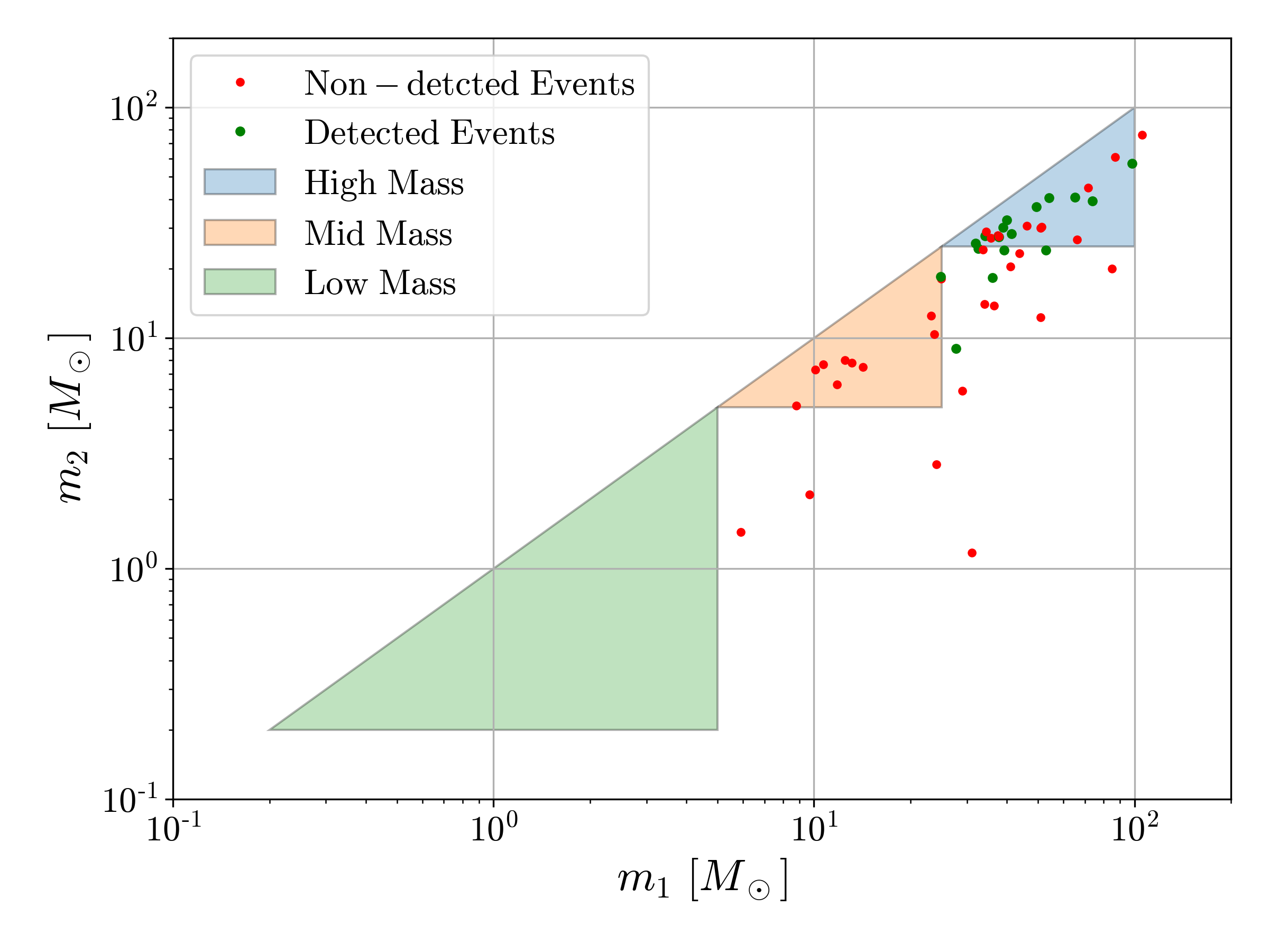
Figure 1: Definition of the search regions in the $m_{1}-m_{2}$ mass plane. The dots indicate the masses of the binary systems corresponding to the GWTC-3 catalog, in green those selected by the CNNs in this work and in red those which are not.

The rest of the CBC event parameters are homogeneously distributed, as indicated in Table 1. This results into signal grids with ${\cal O}(250,000)$ different generated signals in each mass region.

Parameters	Mass range
	Low	Intermediate	High
$m_{1}$, $m_{2}$ [M$\odot$]	[0.2, 5]	[5, 25]	[25, 100]
$D_{\rm{L}}$ [Mpc]	[1, 100]	[1, 1000]	[100, 1400]
$\psi$ [rad]	[0, $\frac{\pi}{2}$]	[0, $\frac{\pi}{2}$]	[0, $\frac{\pi}{2}$]
$\theta_{JN}$ [rad]	[0, $\pi$]	[0, $\pi$]	[0, $\pi$]
$\alpha$ [rad]	[0, 2$\pi$]	[0, 2$\pi$]	[0, 2$\pi$]
$\delta$ [rad]	[0, $\pi$]	[0, $\pi$]	[0, $\pi$]

Table 1: Signal generation parameters in each of the three signal regions. Here $m_{1}$ and $m_{2}$ are the black hole masses in the binary system, computed in the detector frame, with $m_{1}>m_{2}$; $D_{L}$ is the luminosity distance; $\psi$ denotes the inclination of the orbit with respect to the line of sight; $\theta_{JN}$ is the polarization of the GW; and $\alpha$ and $\delta$ are the right ascension and declination, respectively.

In order to control the duration of the signals, a low frequency threshold of 80 Hz is applied to the signals in the low- and intermediate-mass regions. For the high-mass region, this threshold is reduced to 25 Hz. The signals duration is limited to five seconds counting backwards from the merger time to remove low frequency components that might confuse the neural network. The generated signals are randomly placed within five second windows of data from each interferometer before being processed. Background and background plus signal segments are whitened following the same prescription as in Ref. [16]. The whitened segments are used to produce spectrograms using $Q$-transforms [17] with 400 bins in time and 100 bins in frequency. Finally, the images are processed such that their content has zero average and variance equal to one.

3 Neural network definition and training

As in previous studies, we adopted a deep CNN ResNet-50 with a 50-layer architecture, as described in Ref. [18]. Binary cross-entropy was used as a loss function along with Adam as the optimizer [19]. The CNN training was based on the first O3a data period. No attempt was made to carry out a new training process for the O3b data since the sensitivity of the instruments remained stable during the whole O3 observation period [20, 21]. A total of four CNNs per mass range were trained covering all the combinations of interferometer inputs: H1-L1, H1-V1, L1-V1 and the triple combination, H1-L1-V1. The use of single interferometers as input to the CNNs was discarded due to the lower performance already observed in the past compared to the use of multiple inputs. Each neural network is trained for up to 12 epochs and the one with the lowest error over the validation set was selected. In all cases the training showed a stable behaviour. A further improvement of the global sensitivity is achieved by combining the outputs of the separate CNNs into a global discriminant. Such combination provides an additional tool for suppressing glitches in the data affecting independently the interferometers and in different time stamps. As in the case of Ref. [6], a simple average of the H1-L1-V1, H1-L1, L1- V1, and H1-V1 CNN outputs has been considered. As shown in Fig. 2, this translates into a better separation of the background and signal and a decrease in the amount of false positives detected by the neural networks.

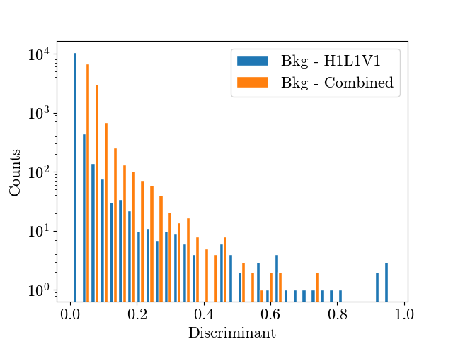
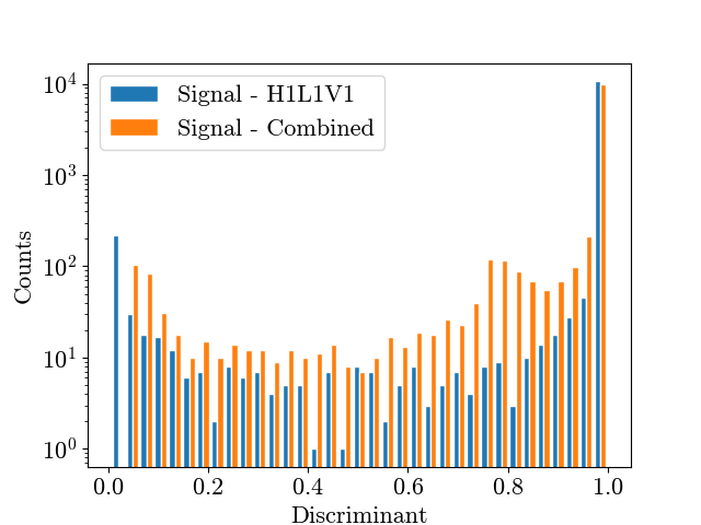
Figure 2: Comparison of the neural network discriminants for (left) background data and (right) simulated signals using the arithmetic mean of all the CNN outputs and only the H1-L1-V1 combination.

The performance of the neural networks is presented in Fig. 3 in terms of the receiver operating characteristic (ROC) curves for the separate CNNs and their combination, representing the true positive (TP) versus the false positive (FP) rates. The best performance is achieved by the high mass neural network, reaching high TP values at low FP. This is to a large extent expected since the high-mass signals are generally louder and more visible in the instruments.

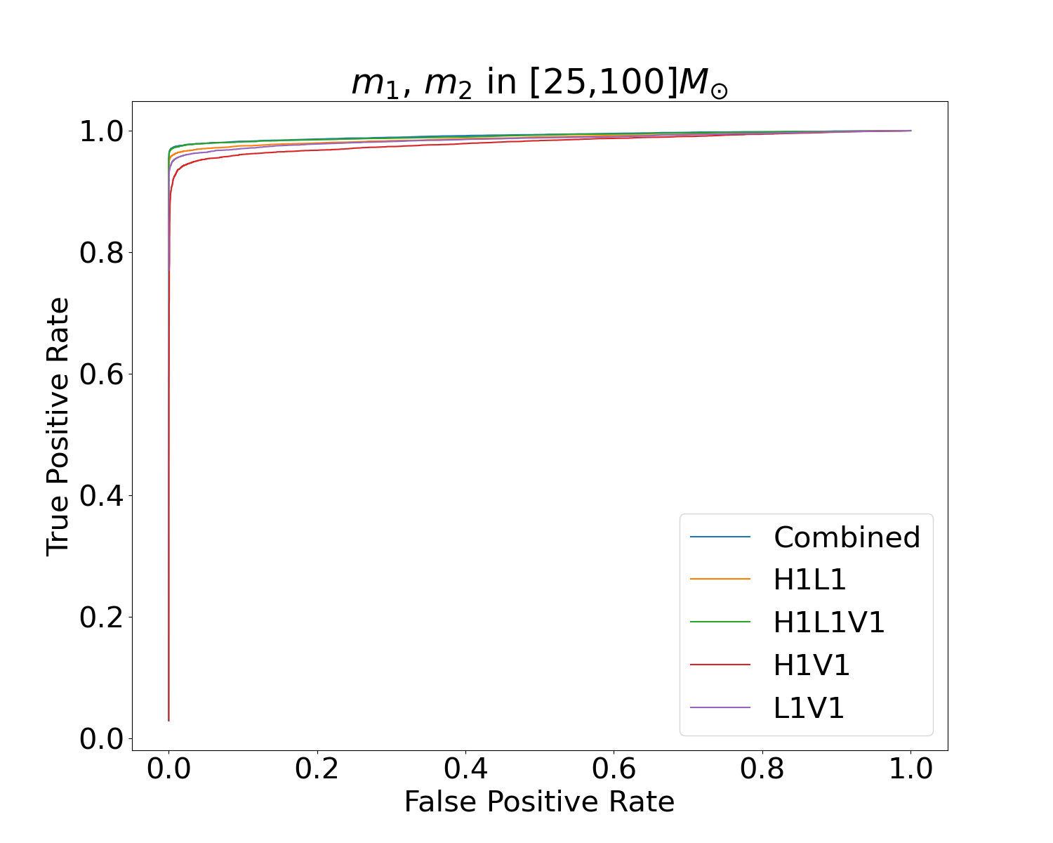
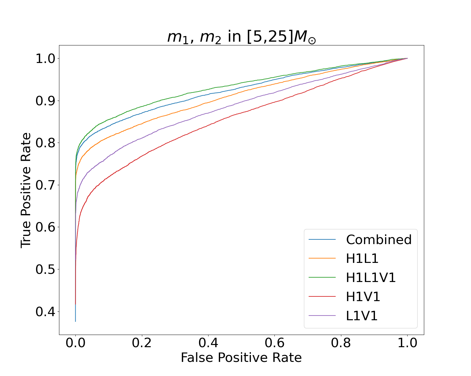
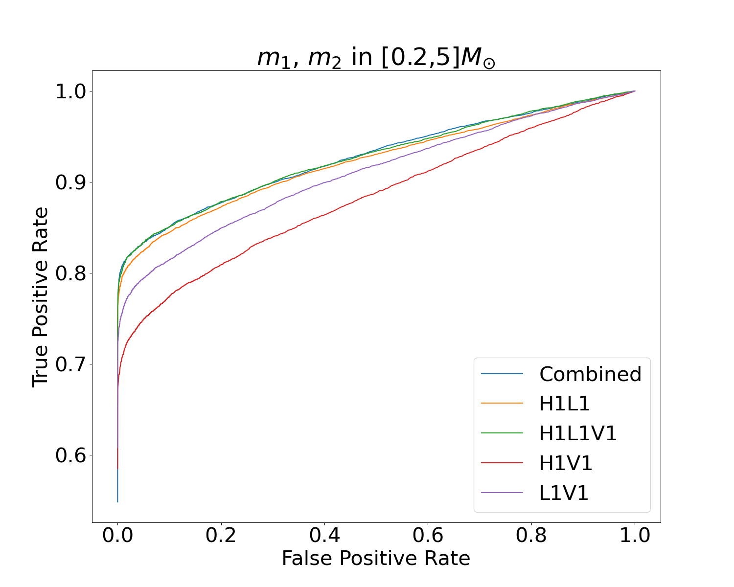
Figure 3: The ROC curves for the different CNNs including different inputs and for (top-left) high-mass; (top-right) intermediate-mass; and (bottom) low-mass regions.

As already mentioned, for each image the CNN discriminant is associated to a FAR value, and the claim for observing a CBC candidate is determined by a predefined FAR threshold. The FAR is estimated as a function of the discriminant of the CNN and is defined as ${\rm{FAR(\eta)}}=N(\eta)/T$, where $\eta\in[0,1]$ is the CNN discriminant, $N(\eta)$ is the number of events with a CNN discriminant above or equal to $\eta$ and $T$ the period of time analysed. In order to effectively increase the time considered in the FAR calculation, thus reaching very low FAR values, the time slide technique [22] is used. This allows accumulating $O(10^{9})$ images (of 5 s of duration each) and accessing FAR values down to $1/152.6$ years^-1. Using this method, we will consider a possible CBC detection when the combined CNN discrimination has an associated FAR value lower than either one event per year or one event per week, where the latter is used to explore a looser selection more adequate for an online implementation of the algorithm, while maintaining the fake rate at a tenable level.

4 Injection tests

Signals with known parameters and signal-to-noise ratios ($\rho$) are injected in real data to understand the performance of the neural networks. The injected signals follow the same distribution as the ones used during the training but sampled uniformly in comoving volume, in agreement with the observed distribution of galaxies in the universe, and the masses are converted into the source frame assuming Planck15 [23] cosmology from the Astropy [24] Python package.

For each GW signal, the value for $\rho$ is computed following the prescription in Ref. [1] solving the integral

$$\rho^{2}=\int_{f_{\rm{min}}}^{f_{\rm{max}}}df\ |h(f)^{2}|/S_{n}(f),$$ (1)

in the frequency domain $(f)$, where $|h(f)^{2}|$ denotes the signal and $S_{n}(f)$ is the power spectral density of the background. We define the network signal-to-noise ratio (SNR), $\mathrm{SNR_{net}}$, as

$$\mathrm{SNR_{net}}=\sum_{i}{\rho_{i}^{2}},$$ (2)

where $i$ is an index that runs over the different interferometers. A total of 32,000 injections per NN were performed. Figure 4 shows the fraction of GW signals identified by the CNNs as a function of $\mathrm{SNR_{net}}$ for the combination of all the neural networks in the different mass regions and for the two FAR thresholds considered. As expected, a looser FAR requirement translates into an improved detection efficiency at a given SNR.

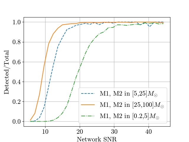
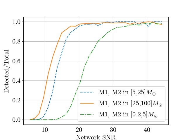
Figure 4: Efficiency as a function of the network SNR corresponding to the combination of all the NNs in each of the mass ranges and for a FAR threshold of (left) one event per week and (right) one event per year.

In the case of a FAR threshold of one event per week, both the high-mass and intermediate-mass neural networks show good efficiency and are almost fully efficient at network SNRs above 20. The low-mass range network instead only becomes fully efficient at network SNRs above 39. This is attributed to the difficulty in detecting low-mass signals not always visible in the images. The same tendency is observed for a FAR threshold of one event per year although the efficiency curve shows a more moderate increase with increasing SNR. Table 2 collects the values of $\mathrm{SNR_{net}}$ for different efficiency values.

FAR threshold of 1 event per week
Mass Range	$\mathrm{SNR_{net}}(50\%)$	$\mathrm{SNR_{net}}(80\%)$	$\mathrm{SNR_{net}}(99\%)$
High	10	12	20
Intermediate	12	15	24
Low	20	24	39
FAR threshold of 1 event per year
Mass Range	$\mathrm{SNR_{net}}(50\%)$	$\mathrm{SNR_{net}}(80\%)$	$\mathrm{SNR_{net}}(99\%)$
High	12	15	28
Intermediate	14	16	28
Low	21	25	41

Table 2: Values of network SNR at given detection efficiencies for the different CNNs and a FAR threshold of 1 event per week and 1 event per year (see body of the text).

Figure 5 presents the efficiency for event detection as a function of the chirp mass, defined as $\mathcal{M}_{c}\equiv\frac{(M_{1}M_{2})^{3/5}}{(M_{1}+M_{2})^{1/5}}$, separately for each mass range. A FAR threshold of one event per week is used in this case. In general, the detection efficiency increases with increasing the chirp mass. In the case of the high-mass range, the CNN efficiency increases from 50$\%$ at 20 $\rm{M\textsubscript{$\odot$}}$ and $90\%$ at 50 $\rm{M\textsubscript{$\odot$}}$ to 98$\%$ at 75 $\rm{M\textsubscript{$\odot$}}$. In the intermediate-mass range, the CNN shows a marginal efficiency at 5 $\rm{M\textsubscript{$\odot$}}$ which increases almost linearly reaching a value of 70$\%$ at 19 $\rm{M\textsubscript{$\odot$}}$. Finally, in the low-mass range, the CNN efficiency increases from 10$\%$ at 1 $\rm{M\textsubscript{$\odot$}}$ and 50$\%$ at 2 $\rm{M\textsubscript{$\odot$}}$ to 85$\%$ at 4 $\rm{M\textsubscript{$\odot$}}$. As expected, the CNN performance is limited at low chirp mass. This indicates that the NNs easily recognize sharp features in higher mass signals and somehow fail to detect low tails in the spectrograms associated with low-mass GW signals.

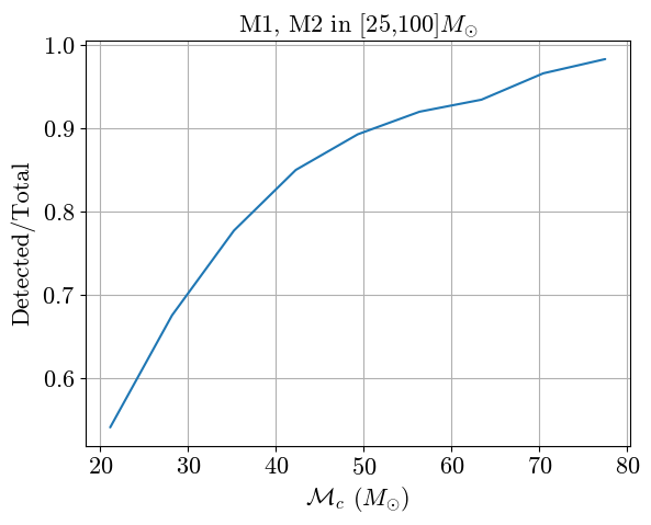
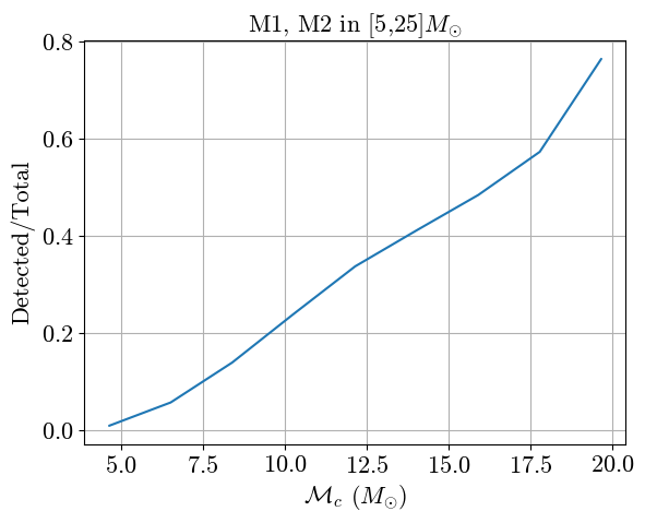
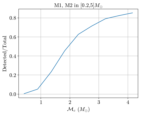
Figure 5: Detection efficiency of the CNNs as a function of the chirp mass corresponding to a FAR threshold of one event per week in (top-left) the high-mass (top-right) the intermediate-mass and (bottom) the low-mass regions.

5 Results

The CNN global discriminating outputs in the different mass ranges, defined as the average of the corresponding H1-L1-V1, H1-L1, L1-V1, and H1-V1 CNN outputs, are used to search for CBC signals. Here we limit ourselves to the analysis of the data for which all the three interferometers were declared in science mode. A slicing window of five seconds duration was used in steps of 2.5 seconds (leading to a 50$\%$ overlap between consecutive images) for each of the interferometers. A scan over the data using different global discriminating values in the range between 0 and 1 is performed. In each case, the corresponding FAR is computed. Figure 6 shows the resulting inverse FAR (IFAR) distributions in the separate mass ranges, in units of years, compared to the expected yields of noise events following Poisson probability distributions.

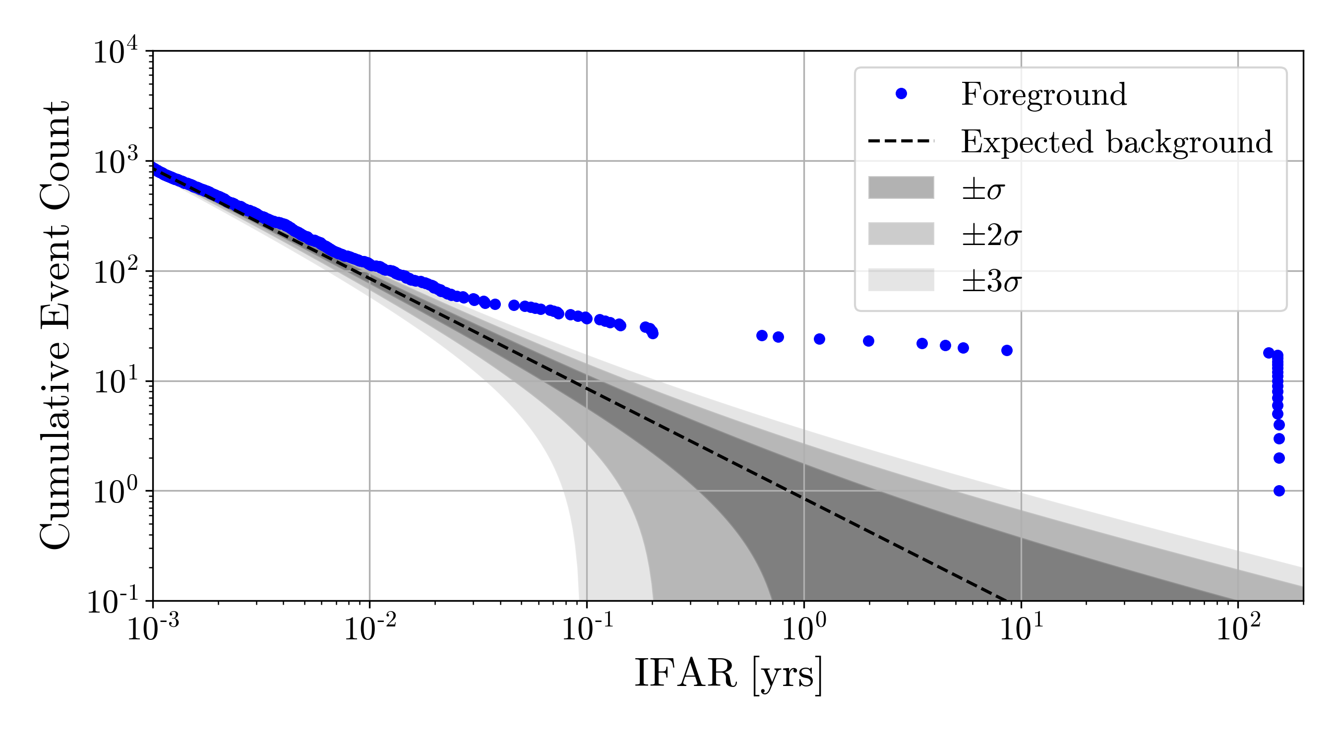
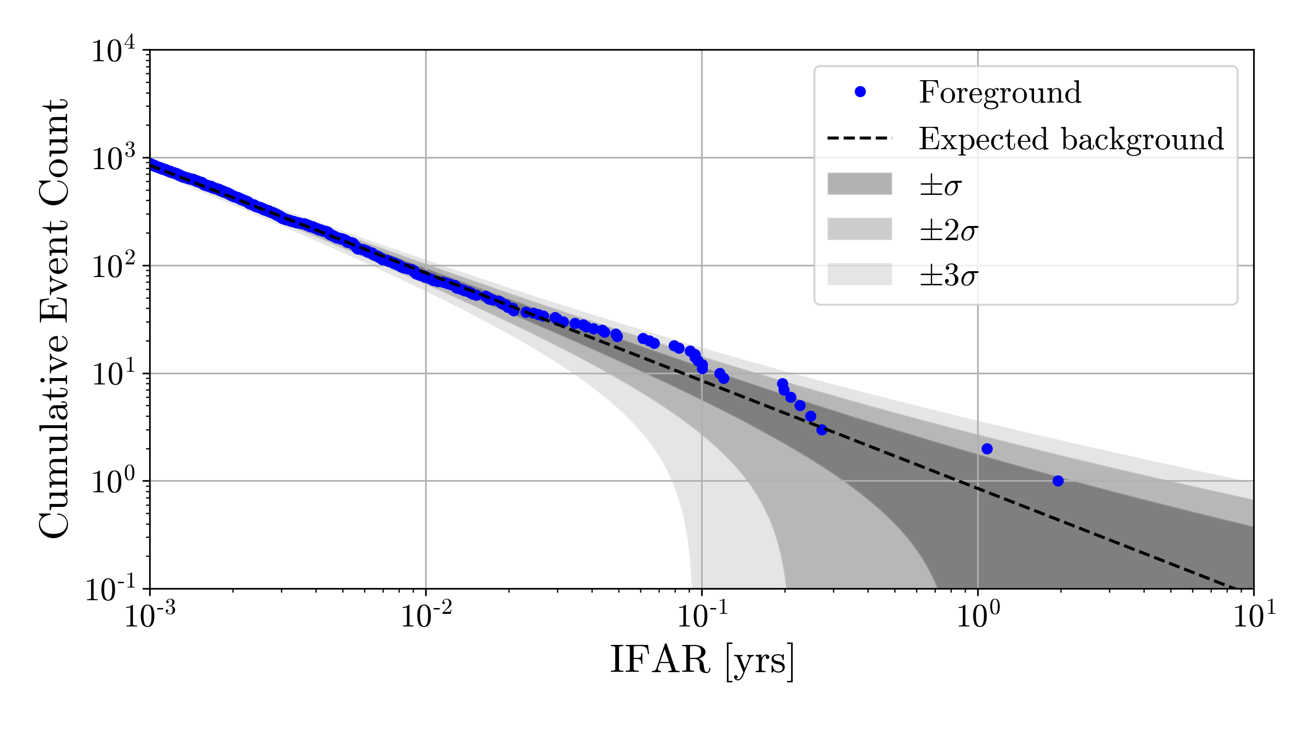
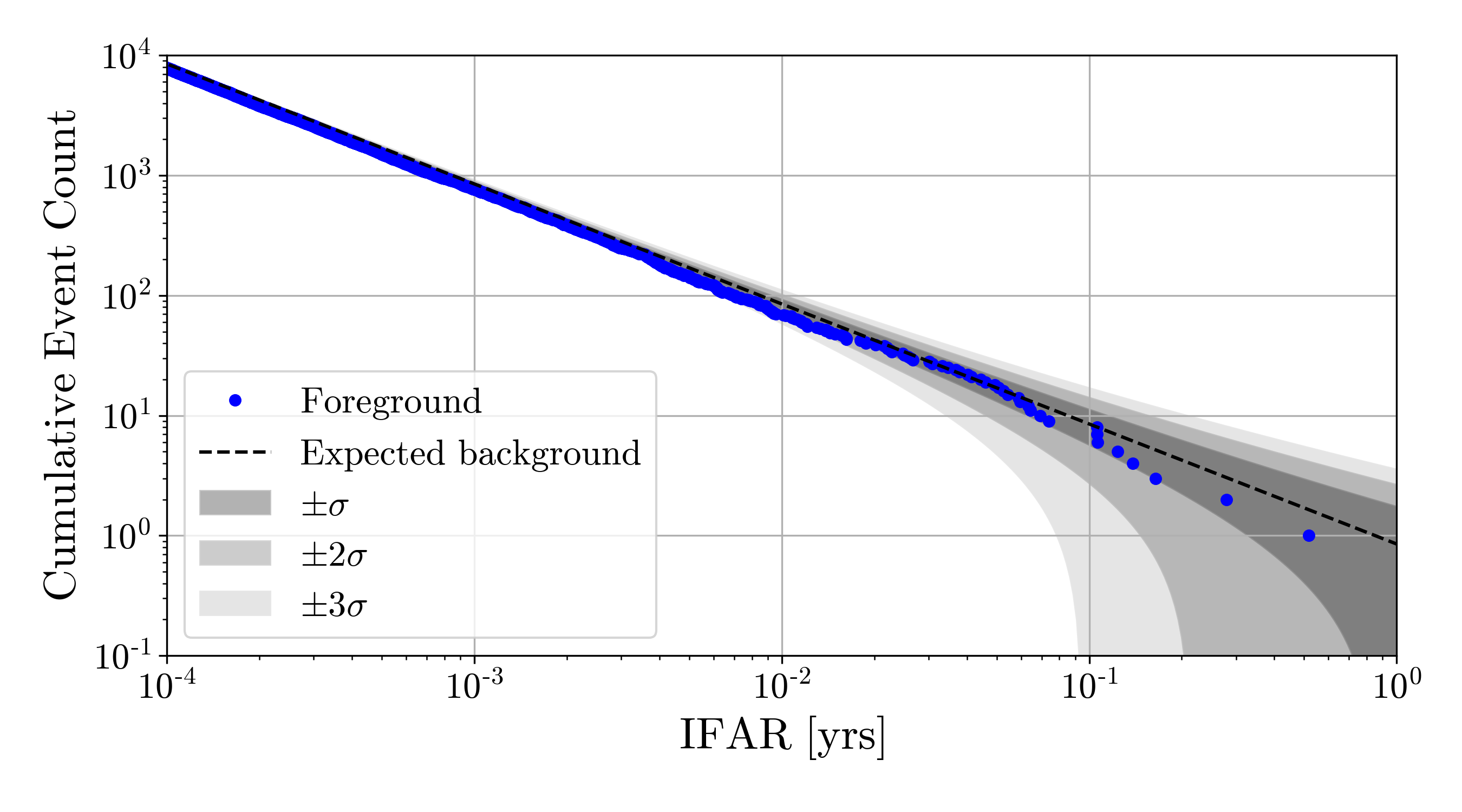
Figure 6: The measured IFAR distributions (dots) for O3 data for the different CNNs in the (top-left) high-mass (top-right) intermediate-mass and (bottom) low-mass regions. The results are compared to the background only expectations (dashed lines) and the corresponding $\pm$1$\sigma$, $\pm$2$\sigma$ and $\pm$3$\sigma$ uncertainty bands.

In the high-mass range an excess of detections above the only-noise prediction is observed. This excess is attributed to the detection of CBC events present in the LIGO/Virgo catalog. It vanishes once the CBC events are excluded from the data. No excess of events above the only-noise prediction is observed in the other mass regions.

Only 51 out of the 90 events from the LIGO/Virgo catalog are inside the part of the data analysed here, with all the three interferometers in science mode. Our CNNs, using a FAR threshold of 1 event per week, detect 26 events, corresponding to an efficiency of about $50\%$. However, this efficiency also includes CBC events out of the mass range used during the CNN training. Out of the 35 catalog events with chirp masses within our CNN training range, 24 events are detected, corresponding to a detection efficiency of $\approx 70\%$, close to the value anticipated by the signal injection studies.

Figure 7 presents the correlation between the network SNR and the chirp mass. As anticipated, the CNN detections are clustered at large SNR and large masses. Finally, A collects the numerical results for the subset of O3 CBC events for which all the three detectors were in science mode. Improving the detection efficiency for a given FAR rate beyond the observed results using CNNs and two-dimensional images would require the suppression of glitches using dedicated algorithms, beyond the scope of this study.

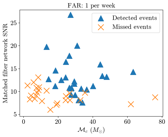
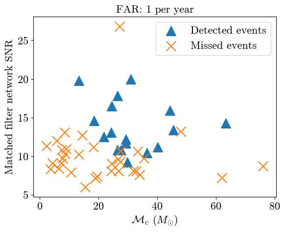
Figure 7: The network SNR versus the chirp mass for the GWTC-3 catalog events with all the three detectors were in science mode. The results are shown for FAR values of one event per week (left) and one event per year (right). The crosses indicate events missed by the CNN and the triangles denote CNN detected events.

6 Summary

We present an update on the search for the coalescence of compact binary mergers using LIGO/Virgo data and convolutional neural networks based on two-dimensional images in time and frequency as input. The analysis is performed in three separate mass regions covering the mass range 0.2 $\rm{M\textsubscript{$\odot$}}$ to 100 $\rm{M\textsubscript{$\odot$}}$. A scan over the O3 LIGO/Virgo data set, using a fake rate threshold for claiming detection of at most one event per week, leads to the detection of about $50\%$ of the O3 catalog events. Once the search is limited to the catalog events within the mass range used for neural networks training, the detection efficiency increases up to about 70$\%$. A further improvement in the search efficiency, using the same algorithms, will require the implementation of new criteria for the suppression of detector glitches.

References

Appendix A CNN results

Table 3 collects the obtained CNN discriminants and the corresponding FAR values for the O3 events. Only the 51 events with the three detectors in science mode have been considered. Results are provided for all the three CNNs corresponding to high-mass, intermediate-mass, and low-mass ranges, as discussed in the body of the text.

Results CNN scan over O3 events
Event	Discriminant			FAR (yrs-1)
	high-mass	low-mass	intermediate-mass	high-mass	low-mass	intermediate-mass
GW190403_051519	0.79	0.18	0.5	37.34	$>$100	$>$100
GW190408_181802	1.0	0.2	0.88	0.01	$>$100	$>$100
GW190412_053044	0.99	0.24	0.9	0.01	$>$100	$>$100
GW190413_052954	0.77	0.15	0.73	68.62	$>$100	$>$100
GW190413_134308	0.88	0.29	0.41	5.01	$>$100	$>$100
GW190426_152155	0.06	0.55	0.22	$>$100	$>$100	$>$100
GW190426_190642	0.28	0.22	0.26	$>$100	$>$100	$>$100
GW190503_185404	0.99	0.3	0.76	0.01	$>$100	$>$100
GW190512_180714	0.79	0.18	0.8	39.74	$>$100	$>$100
GW190513_205428	1.0	0.14	0.76	0.01	$>$100	$>$100
GW190517_055101	0.96	0.16	0.43	0.19	$>$100	$>$100
GW190519_153544	1.0	0.18	0.4	0.01	$>$100	$>$100
GW190521_030229	1.0	0.15	0.49	0.01	$>$100	$>$100
GW190701_203306	1.0	0.15	0.49	0.01	$>$100	$>$100
GW190706_222641	1.0	0.22	0.47	0.01	$>$100	$>$100
GW190720_000836	0.07	0.14	0.58	$>$100	$>$100	$>$100
GW190725_174728	0.08	0.25	0.65	$>$100	$>$100	$>$100
GW190727_060333	1.0	0.16	0.76	0.01	$>$100	$>$100
GW190728_064510	0.17	0.54	0.97	$>$100	$>$100	5.035
GW190803_022701	0.85	0.16	0.35	10.01	$>$100	$>$100
GW190805_211137	0.81	0.2	0.46	26.52	$>$100	$>$100
GW190828_063405	1.0	0.24	0.64	0.01	$>$100	$>$100
GW190828_065509	0.17	0.2	0.46	$>$100	$>$100	$>$100
GW190915_235702	0.99	0.17	0.54	0.01	$>$100	$>$100
GW190916_200658	0.68	0.17	0.39	$>$100	$>$100	$>$100
GW190917_114630	0.05	0.21	0.2	$>$100	$>$100	$>$100
GW190924_021846	0.05	0.16	0.56	$>$100	$>$100	$>$100
GW190926_050336	0.75	0.2	0.2	$>$100	$>$100	$>$100
GW190929_012149	0.77	0.23	0.3	76.78	$>$100	$>$100
GW191105_143521	0.05	0.2	0.62	$>$100	$>$100	$>$100
GW191113_071753	0.07	0.19	0.33	$>$100	$>$100	$>$100
GW191127_050227	1.0	0.19	0.65	0.01	$>$100	$>$100
GW191215_223052	0.81	0.15	0.49	32.00	$>$100	$>$100
GW191219_163120	0.09	0.16	0.34	$>$100	$>$100	$>$100
GW191230_180458	0.98	0.17	0.63	0.51	$>$100	$>$100
GW200115_042309	0.08	0.17	0.23	$>$100	$>$100	$>$100
GW200129_065458	0.95	0.15	0.62	1.56	$>$100	$>$100
GW200202_154313	0.08	0.33	0.6	$>$100	$>$100	$>$100
GW200208_130117	0.99	0.27	0.38	0.22	$>$100	$>$100
GW200208_222617	0.51	0.22	0.44	$>$100	$>$100	$>$100
GW200209_085452	0.78	0.23	0.46	86.13	$>$100	$>$100
GW200210_092254	0.08	0.39	0.62	$>$100	$>$100	$>$100
GW200216_220804	0.47	0.17	0.47	$>$100	$>$100	$>$100
GW200219_094415	0.8	0.15	0.39	45.064	$>$100	$>$100
GW200220_061928	0.13	0.18	0.31	$>$100	$>$100	$>$100
GW200224_222234	1.0	0.25	0.95	0.01	$>$100	12.61
GW200308_173609	0.23	0.2	0.31	$>$100	$>$100	$>$100
GW200311_115853	1.0	0.18	0.94	0.01	$>$100	23.00
GW200316_215756	0.2	0.16	0.19	$>$100	$>$100	$>$100
GW200322_091133	0.17	0.14	0.48	$>$100	$>$100	$>$100

Table 3: CNN discriminants and the corresponding FAR values for the O3 events with all the three detectors in science mode.

References

- [1] Hunter Gabbard, Michael Williams, Fergus Hayes, and Chris Messenger. Matching matched filtering with deep networks for gravitational-wave astronomy. Phys. Rev. Lett., 120:141103, Apr 2018.
- [2] Daniel George and E. A. Huerta. Deep neural networks to enable real-time multimessenger astrophysics. Phys. Rev. D, 97(4):044039, 2018.
- [3] Timothy D. Gebhard, Niki Kilbertus, Ian Harry, and Bernhard Schölkopf. Convolutional neural networks: A magic bullet for gravitational-wave detection? Phys. Rev. D, 100(6), Sep 2019.
- [4] Daniel George and E. A. Huerta. Deep learning for real-time gravitational wave detection and parameter estimation: Results with advanced ligo data. Phys. Lett. B, 778:64–70, Mar 2018.
- [5] Alexis Menéndez-Vázquez, Machiel Kolstein, Mario Martínez, and Lluïsa-Maria Mir. Searches for compact binary coalescence events using neural networks in the ligo/virgo second observation period. Phys. Rev. D, 103(6):062004, 2021.
- [6] Marc Andrés-Carcasona, Alexis Menéndez-Vázquez, Mario Martínez, and Lluïsa-Maria Mir. Searches for mass-asymmetric compact binary coalescence events using neural networks in the ligo/virgo third observation period. Phys. Rev. D, 107:082003, Apr 2023.
- [7] Massimiliano Razzano and Elena Cuoco. Image-based deep learning for classification of noise transients in gravitational wave detectors. Class. Quantum Grav., 35(9):095016, Apr 2018.
- [8] Rahul Biswas et al. Application of machine learning algorithms to the study of noise artifacts in gravitational-wave data. Phys. Rev. D, 88(6), Sep 2013.
- [9] Marco Cavaglia, Kai Staats, and Teerth Gill. Finding the origin of noise transients in ligo data with machine learning. Commun. Comput. Phys., 25(4), 2019.
- [10] Marc Andrés-Carcasona, Mario Martínez, and Lluïsa-Maria Mir. Fast bayesian gravitational wave parameter estimation using convolutional neural networks. Monthly Notices of the Royal Astronomical Society, 527(2):2887–2894, 2023.
- [11] R. Abbott et al. Open data from the first and second observing runs of advanced ligo and advanced virgo. SoftwareX, 13:100658, 2021.
- [12] Samantha A. Usman et al. The pycbc search for gravitational waves from compact binary coalescence. Class. Quantum Grav., 33(21):215004, 11 2016.
- [13] Alexander H. Nitz, Thomas Dent, Tito Dal Canton, Stephen Fairhurst, and Duncan A. Brown. Detecting binary compact-object mergers with gravitational waves: Understanding and improving the sensitivity of the pycbc search. The Astrophysical Journal, 849(2):118, 2017.
- [14] Alex Nitz et al. gwastro/pycbc: Pycbc release v1. 16.11. Zenodo, 2020.
- [15] Sebastian Khan, Katerina Chatziioannou, Mark Hannam, and Frank Ohme. Phenomenological model for the gravitational-wave signal from precessing binary black holes with two-spin effects. Phys. Rev. D, 100(2), Jul 2019.
- [16] Benjamin P. Abbott et al. A guide to ligo–virgo detector noise and extraction of transient gravitational-wave signals. Class. Quantum Grav., 37(5):055002, 2020.
- [17] Judith C. Brown. Calculation of a constant q spectral transform. The Journal of the Acoustical Society of America, 89(1):425–434, 1991.
- [18] Kaiming He, Xiangyu Zhang, Shaoqing Ren, and Jian Sun. Deep residual learning for image recognition. CoRR, abs/1512.03385, 2015.
- [19] Diederik P. Kingma and Jimmy Lei Ba. Adam: A Method for Stochastic Optimization. 3rd International Conference on Learning Representations, ICLR 2015 - Conference Track Proceedings, 12 2014.
- [20] R. Abbott et al. GWTC-2: Compact Binary Coalescences Observed by LIGO and Virgo During the First Half of the Third Observing Run. https://arxiv.org/abs/2010.14527, 2020.
- [21] The LIGO Scientific Collaboration, The Virgo Collaboration, The KAGRA Collaboration: R. Abbot, et al. GWTC-3: Compact Binary Coalescences Observed by LIGO and Virgo During the Second Part of the Third Observing Run. https://arxiv.org/abs/2111.03606, 2021.
- [22] B. Abbott et al. Search for gravitational waves from galactic and extra-galactic binary neutron stars. Phys. Rev. D, 72(8):23, 10 2005.
- [23] P. A. R. Ade et al. Planck 2015 results. xiii. cosmological parameters. Astron. Astrophys., 594:A13, 2016.
- [24] Astropy Collaboration and Astropy Contributors. The astropy project: Building an open-science project and status of the v2.0 core package. The Astronomical Journal, 156(3):123, aug 2018.