Pretraining and the Lasso
2Department of Electrical Engineering
3Department of Statistics
4 Department of Biochemistry
5 Institute for Computational and Mathematical Engineering
Stanford University)
Abstract
Pretraining is a popular and powerful paradigm in machine learning. As an example, suppose one has a modest-sized dataset of images of cats and dogs, and plans to fit a deep neural network to classify them from the pixel features. With pretraining, we start with a neural network trained on a large corpus of images, consisting of not just cats and dogs but hundreds of other image types. Then we fix all of the network weights except for the top layer (which makes the final classification) and train (or “fine tune”) those weights on our dataset.111 Typically only the top-layer is fine-tuned, but more layers can be fine-tuned, if computationally feasible. This is an area of active research. This often results in dramatically better performance than the network trained solely on our smaller dataset.
In this paper, we ask the question “Can pretraining help the lasso?”. We develop a framework for the lasso in which an overall model is fit to a large set of data, and then fine-tuned to a specific task on a smaller dataset. This latter dataset can be a subset of the original dataset, but does not need to be. We find that this framework has a wide variety of applications, including stratified models, multinomial targets, multi-response models, conditional average treatment estimation and even gradient boosting.
In the stratified model setting, the pretrained lasso pipeline estimates the coefficients common to all groups at the first stage, and then group-specific coefficients at the second “fine-tuning” stage. We show that under appropriate assumptions, the support recovery rate of the common coefficients is superior to that of the usual lasso trained only on individual groups. This separate identification of common and individual coefficients can also be useful for scientific understanding.
Keywords: Supervised Learning, Pretraining, Lasso, Transfer learning
1 Introduction
Pretraining is a popular and powerful tool in machine learning. As an example, suppose you want to build a neural net classifier to discriminate between images of cats and dogs, and suppose you have a labelled training set of say 500 images. You could train your model on this dataset, but a more effective approach is to start with a neural net trained on a much larger corpus of images, for example IMAGENET which contains 1000 object classes and 1,281,167 training images. The weights in this fitted network are then fixed, except for the top layer which makes the final classification of dogs vs cats; finally, the weights in this top layer are refitted using our training set of 500 images. This approach is effective because the initial network, learned on a large corpus, can discover potentially predictive features for our discrimination problem. This paper asks: is there a version of pretraining for the lasso? We propose such a framework.
Our motivating example came from a study carried out in collaboration with Genentech (McGough et al., 2023). The authors curated a large pancancer dataset, consisting of 10 groups of patients with different cancers, approximately patients in all. Some of the cancer classes are large (e.g. breast, lung) and some are smaller (e.g. head and neck). The goal is to predict survival times from a large number of features, (labs, genetics, ), approximately 50,000 in total. They compare two approaches: (a) a “pancancer model”, in which a single model is fit to the training set and used to make predictions for all cancer classes: and (b) separate (class specific) models are trained for each class and used to make predictions for that class.
The authors found that the two approaches produced very similar results, with the pancancer model offering a small advantage in test set C-index for the smaller classes (such as head and neck cancer). Presumably this occurs because of the insufficient sample size for fitting a separate head and neck cancer model, so that “borrowing strength” across a set of different cancers can be helpful.
This led us to consider a framework where the overall (pancancer) model can be blended with individual models in an adaptive way, a paradigm that is somewhat closely related to the ML pretraining mentioned above. It also has similarities to transfer learning.
This paper is organized as follows. In Section 2 we review the lasso, describe the pretrained lasso, and show the result on the TCGA pancancer dataset. Section 3 discusses related work. In section 4 we demonstrate the generality of the idea, detailing a number of different “use cases”. We discuss a method for learning the input groups from the data itself in Section 5. In Section 6 we study the performance of the pretrained lasso in different use cases on simulated data. Real data examples are shown throughout the paper, including application to cancer, genomics, and chemometrics. Section 7 establishes some theoretical results for the pretrained lasso. In particular we show that under the “shared/ individual model” discussed earlier, the new procedure enjoys improved rates of support recovery, as compared to the usual lasso. We move beyond linear models in Section 10, illustrating an application of the pretrained lasso to gradient boosting. We examine our use of cross-validation in Section 11 and end with a discussion in Section 12.
2 Pretraining the lasso
2.1 Review of the lasso
For the Gaussian family with data , the lasso has the form
| (1) |
Varying the regularization parameter yields a path of solutions: an optimal value is usually chosen by cross-validation, using for example the cv.glmnet function in the R language package glmnet (Friedman et al., 2010).
Before presenting our proposal, two more background facts are needed. In GLMs and - regularized GLMs, one can include an offset: this is a pre-specified -vector that is included as an additional column to the feature matrix, but whose weight is fixed at 1. Secondly, one can generalize the norm to a weighted norm, taking the form
| (2) |
where each is a penalty factor for feature . At the extremes, a penalty factor of zero implies no penalty and means that the feature will always be included in the model; a penalty factor of leads to that feature being discarded (i.e., never entered into the model).
2.2 Underlying model and intuition
Suppose we express our data as a feature matrix and a target vector , and we want to do supervised learning via the lasso. In the training set, suppose further that each observation falls in one of pre-specified classes, and therefore the rows of our data are partitioned into groups and .
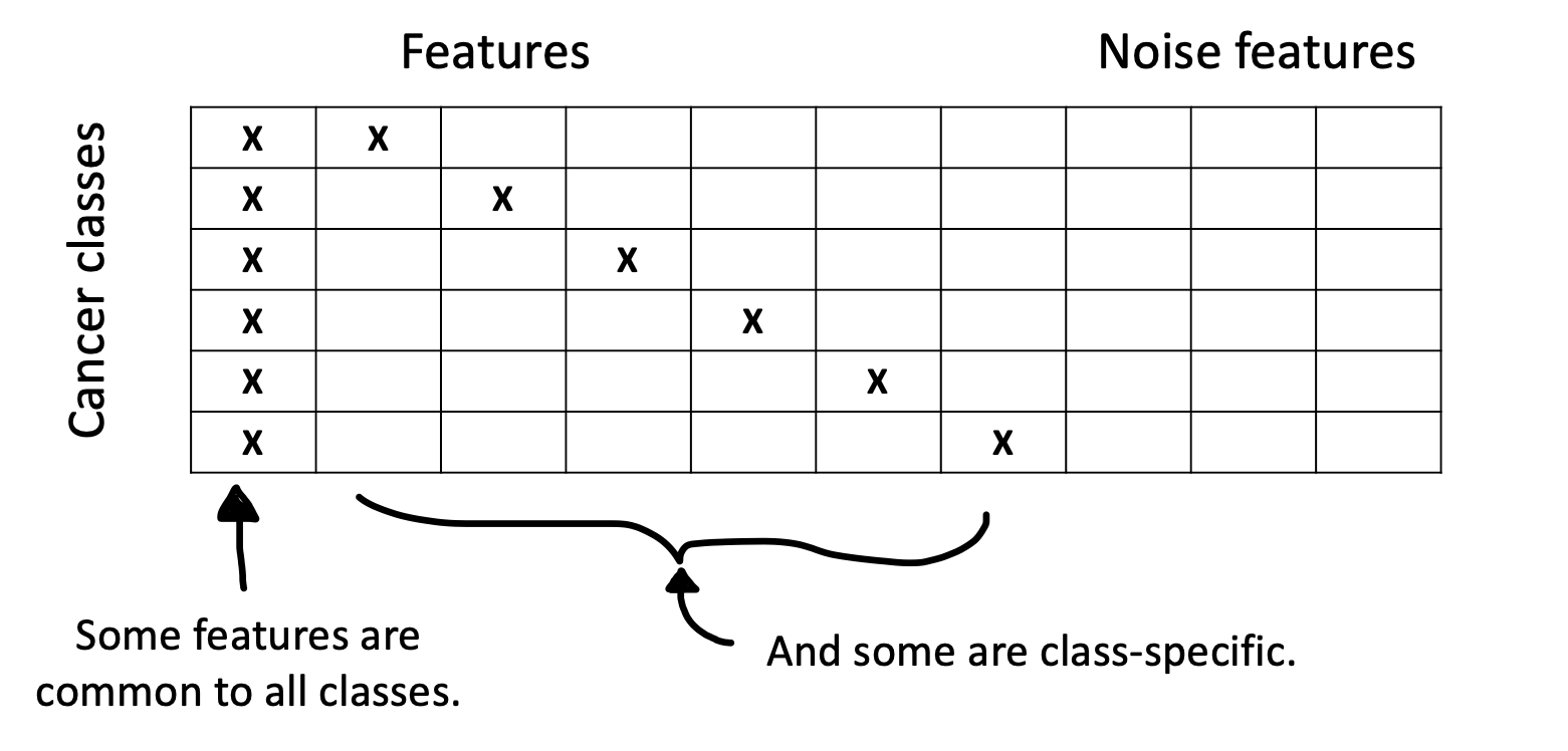
As shown in Figure 1, we imagine that the features are roughly divided into two types: common features that are predictive in most or all classes, and individual features, predictive in one particular class. Finally there are noise features, with little or no predictive power. Our proposal for this problem is a two-step procedure, with the first step aimed at discovering the common features and the second step focused on recovery of the class-specific features.
For simplicity, we assume here that is a Gaussian response ( can also be any member of the GLM family, such as binomial, multinomial, or Cox survival). Our model, a kind of data-shared lasso (Gross & Tibshirani, 2016), has the form:
| (3) |
where is the vector of responses for data in group . Note that is shared across all classes ; this is intended to capture the common features. The class specific captures features that are unique to each class, and may additionally adjust the coefficient values in .
We fit this model in two steps. First, we train a model using all the data. We fit an overall model:
| (4) |
for some choice of (e.g the value minimizing the CV error). Define to be the support set (the nonzero coefficients) of . Now, for each group , we fit a class specific model: we find and such that
| (5) | |||
| (6) |
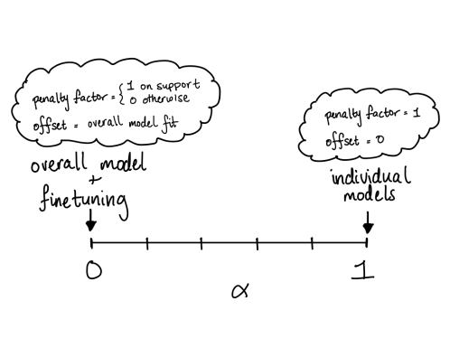
We choose through cross validation, and is a hyperparameter. Notice that when , this very nearly returns the overall model, and when this is equivalent to fitting a class specific model for each class. This property is the result of the inclusion of two terms that interact with (illustrated in Figure 4).
First, the offset in the loss determines how much the prediction from the overall model influences the class specific models. When the response is Gaussian, using this term is the same as fitting a residual: the class specific model uses the target . That is, the class specific model can only find signal that was left over after taking out the overall model’s contribution. When , the class specific model is forced to use the overall model, and when , the overall model is ignored.
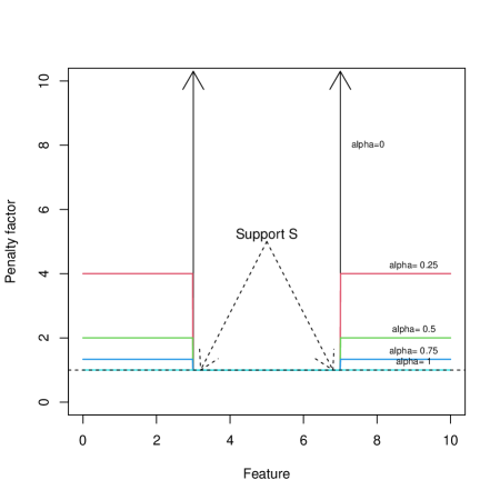
Second, the usual lasso penalty is modified by the penalty factor for each coefficient . This is a function that is on the support of the overall model and off the support (illustrated in Figure 2). When , the penalty factor is off the support , and so the class specific model is only able to use features on the support of the overall model. When , the penalty factor is everywhere, and all variables are penalized equally as in the usual lasso.
Remark 1.
In our numerical experiments and theoretical analysis (Section 7), we find that the transmission of both ingredients— the offset and penalty factor— are important for the success of the method. The offset captures the model fit at the first step, while the penalty factor captures its support.
2.3 The algorithm
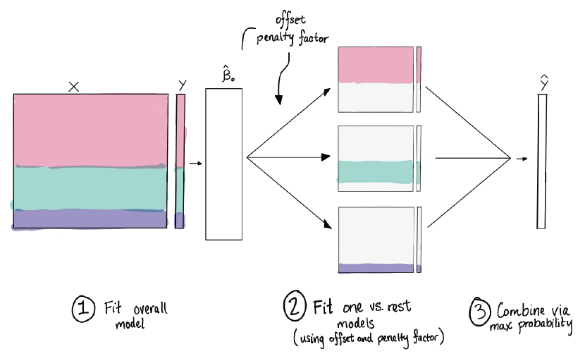
We now summarize the pretrained lasso algorithm discussed above. For clarity we express the computation in terms of the R language package glmnet, although in principal this could be any package for fitting -regularized generalized linear models and the Cox survival model. A roadmap of the procedure is shown in Figure 3. As described in Section 4, our proposed paradigm is far more general: we first describe the simplest case for ease of exposition.
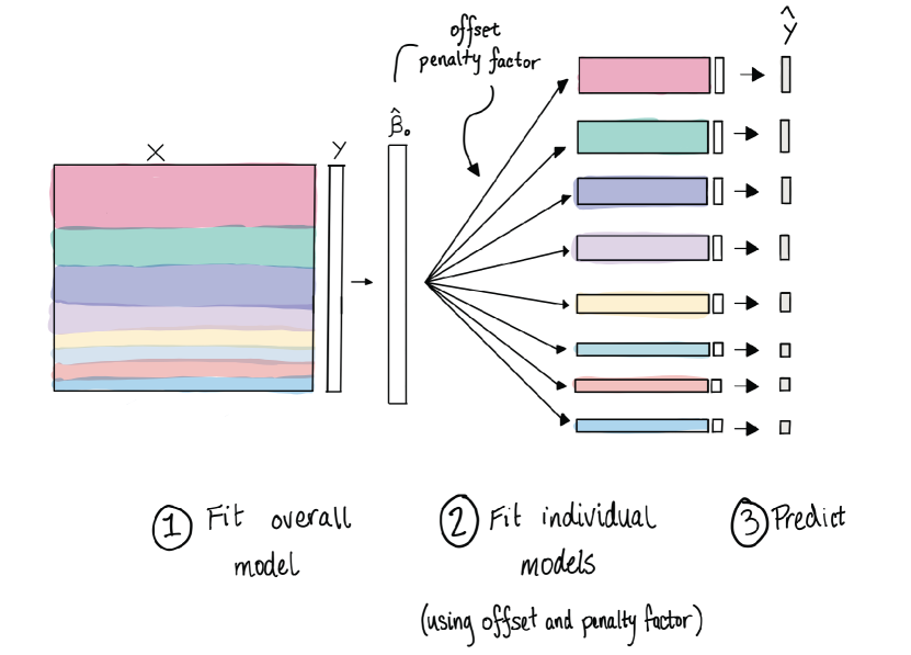
The procedure is a two step process: first, an overall model is fit using all the data. An offset and penalty factor are computed from this model, and these two ingredients are passed on to Step 2, where a class specific model is fit to each class. The class specific model is used for prediction in each class. The two steps are given in detail in Algorithm 1.
-
1.
Fit a single (“overall”) lasso model to the training set, using for example cv.glmnet in the R language. From this, choose a model (weight vector) along the path, using e.g. lambda.min — the value minimizing the CV error.
-
2.
Fix . Define the offset and penalty factor as follows:
-
•
Compute the linear predictor , and define .
-
•
Let be the support set of . Define the penalty factor by .
For each class , fit an individual model using cv.glmnet, and using the offset and penalty.factor defined above. Use these individual models for prediction within each group.
-
•
We again note that when , this is similar to using the overall model for each class: it uses the same support set, but “fine-tunes” the weights (coefficients) to better fit the specific group. When the method corresponds to fitting separate class-specific models. See Figure 4.
Remark 2.
The forms for the offset and penalty factor were chosen so that the family of models, indexed by , captures both the individual and overall models at the extremes. We have not proven that this particular formulation is optimal in any sense, and a better form may exist.
Remark 3.
We can think of the pretrained lasso as a simple form of a Bayes procedure, in which we pass “prior” information — the offset and penalty factor — from the first stage model to the individual models at the second stage.
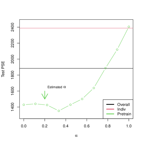
2.4 Simulated example
Figure 5 shows an example with , groups, and the common coefficients have different magnitudes in each group (ranging from to ), and the individual coefficients are or for all , such that the nonzero entries of the s are non-overlapping. A test set of size 5000 was also generated. Shown are the test set prediction squared error for the overall, individual and pretrained lasso models. The arrow indicates the cross-validated choice of for the pretrained lasso, which achieves the lowest PSE among the 3 methods.
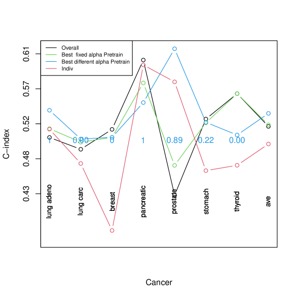
2.5 Example: TCGA PanCancer dataset
At the time of this writing, for logistical reasons, we have not yet applied lasso pretraining to the Genentech pancancer dataset discussed earlier. Instead we applied it to the public domain TCGA pancancer dataset (Goldman et al., 2020). After cleaning and collating the data, we were left with 4037 patients, and 20,531 gene expression values. The patients fell into one of 7 cancer classes as detailed in Table 1. We used a CART survival tree to pre-cluster the 7 classes into 3 classes: (“breast invasive carcinoma”, “prostate adenocarcinoma” , “thyroid carcinoma”), (“lung adenocarcinoma”, “lung squamous cell carcinoma”, “stomach adenocarcinoma”) and “pancreatic adenocarcinoma”
The outcome was PFS (progression-free survival): there were 973 events. For computational ease, we filtered the genes down to the 500 genes having the largest absolute Cox PH score: all methods used this filtered dataset. The data was divided into a training (50%), validation set (25%) and a test set (25%). The validation set was used to select the best values for .
Figure 6 shows the test set C-index values for a number of methods. Table 1 shows the number of non-zero genes from each cancer class, for each model.
| lung adeno | lung carc | breast | pancreatic | prostate | stomach | thyroid | Total | |
|---|---|---|---|---|---|---|---|---|
| Sample size | 283 | 281 | 593 | 98 | 279 | 202 | 282 | 2018 |
| Overall | 25 | |||||||
| PreTrain | 50 | 15 | 15 | 1 | 3 | 1 | 8 | 93 |
| Indiv | 5 | 7 | 1 | 1 | 1 | 19 | 1 | 35 |
We see that the pretrained lasso provides a clear improvement as compared to the overall model, and a small improvement over the individual models. From a biological point of view, the separation of genes into common and cancer-specific types could aid in the understanding of the underlying diseases.
Remark 4.
Suppose we had more than one pancancer dataset (say 10), and as above, we want to predict the outcome in one particular cancer. Emmanuel Candès suggested that one might repeatedly sample one of the 10 datasets, and apply the pretrained lasso to each realization. In this way, one could obtain posterior distributions of model parameters and predictions, to account for the variability in pancancer datasets.
Remark 5.
Pretraining may be useful when the input groups share overlapping — but not identical — features. For example, some features may be measured for just one cancer; this feature may then be used only in the individual model for that cancer (stage 2 of pretraining), while the overall model (stage 1) uses features shared by all groups.
3 Related work
3.1 Data Shared Lasso
Data Shared Lasso (Gross & Tibshirani, 2016) (DSL) is a closely related approach for modeling data with a natural group structure. It solves the problem
| (7) |
That is, it jointly fits an overall coefficient vector that is common across all groups, as well as a modifier vector for each group . The parameter in the penalty term controls the size of , and therefore determines whether the solution should be closer to the overall model (for large) or the individual model (for small).
DSL is analogous to pretrained lasso in many ways. Both approaches fit an “overall” model and “individual” models, and both have a parameter ( or ) to balance between the two. One important difference between DSL and pretraining is the use of penalty.factor in pretraining. For , pretraining encourages the individual models to use the same features that are used by the overall model, but allows them to have different values. DSL has no such restriction relating to the modifier . Additionally, because pretraining is performed in two steps, it is more flexible: for example, researchers with large datasets can train and share overall models that others can use to train an individual model with a smaller dataset.
3.2 Laplacian Regularized Stratified Models
Stratified modeling fits a separate model for each group. Laplacian regularized stratified modeling Tuck & Boyd (2021) incorporates regularization to encourage separate group models to be similar to one another, depending on a user-defined structure indicating similarity between groups. For example, we may expect lymphoma and leukemia to have similar features because they are both blood cancers, and we could pre-specify this when fitting a laplacian regularized stratified model. So, while pretrained lasso uses information from an overall model, laplacian regularized stratified modeling uses known similarities between individual groups.
3.3 Reluctant Interaction Modeling
Reluctant Interaction Modeling Yu et al. (2019) is a method to train a lasso model using both main and interaction effects, while (1) prioritizing main effects and (2) avoiding the computational challenge of training a model using all interaction terms. It uses three steps: in the first, a model is trained using main effects only. Then, a subset of interaction terms are selected based on their correlation with the residual from the first model; the intention is to only consider interactions that may explain the remaining signal. Finally, a model is fit to the residual using the main effects and the selected set of interaction effects. Though it has a different goal than pretraining, Reluctant Interaction Modeling uses a similar algorithm: train an initial model, and then train a second model to the residual from the first, using a subset of features.
3.4 Mixed Effects Models
Mixed effects models jointly find fixed effects (common to all the data) and random effects (specific to individual instances). A linear mixed effect model has the form
| (8) |
where consists of features shared by all instances and consists of features related to individual instances. Both pretrained lasso and mixed effects modeling aim to uncover two components; in pretraining, however and we seek to divide into overall and group-specific components.
4 Pretrained lasso: a wide variety of use cases
We have described the main idea for lasso pretraining, as applied to a dataset with fixed input groupings: a model is fit on a large set of data, an offset and penalty factor are computed, and these components are passed on to a second stage, where individual models are built for each group. It turns out that the pretraining idea for the lasso is a general paradigm, with many different ways that it can be applied. Typically the pipeline has only two steps, as in the example above; but in some cases it can consist of multiple steps, as made clear next.
The common feature of these different “use cases” is the passing of an offset and penalty factor from one model to the next.
Here is a (non-exhaustive) list of potential use cases:
-
1.
Input grouping:
The rows of are partitioned into groups. These groups may be:-
(a) Pre-specified (Section 2.3), e.g. cancer classes, age groups, ancestry groups. The pancancer dataset described above is an example of this use case.
-
(b) Pre-specified but different in training and test sets (Section 4.3), e.g. different train and test patients.
-
(c) Learned from the data via a decision tree (Section 5).
-
-
2.
Target grouping:
Here, there is a natural grouping on the target , and may be:-
(a) binomial or multinomial, and there is one group for each response class.
-
(b) multi-response: is a matrix, and there is one group for each column of (Section 4.1). Two special cases: time-ordered columns, where the same target variable is measured at different points in time, and mixed targets, where the different target columns are of different types, e.g. quantitative, survival, or binary/multinomial. In both cases, the pretrained lasso is applied to each target column in sequence. This is illustrated in Section 8.
-
-
3.
Both input and target groupings: Suppose for example the target is 0-1, multinomial or multi-response, and there is a separate grouping on the rows of , e.g. the rows of are stratified into age groups, and we want to predict cancer class.
-
4.
Conditional average treatment effect estimation. This is similar to the input grouping case (#1 above). Here the groups are defined by the levels of a treatment variable (Section 9).
-
5.
Unlabelled pretraining: Given unlabelled pretraining data, we can use sparse PCA to estimate the support, and use the first principal component as the offset.
Of course, other scenarios are possible.
4.1 Target grouping: binomial, multinomial or multiresponse target
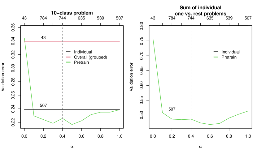
We begin by describing the multinomial (or binomial) setting, and then we extend this to the multiresponse case. Suppose we have response classes and wish to fit a multinomial model. Figure 7 shows an overview of our two-stage procedure. It is much the same as our earlier algorithm, the only difference being the way in which the models are combined at the end. Here is the procedure in detail:
-
1.
At the first stage, let be the coefficient matrix. Fit a grouped multinomial model to all classes (using two-norm penalties on the rows of ).
-
2.
Second stage: for each class , define the offset equal to the th column of . Define to be the support of the th column of . Use penalty factor . Fit a two class model for class vs the rest using the offset and penalty factor.
-
3.
Classify each observation to the class having the maximum probability across all of the one versus rest problems.
This is applied to real data in Section 4.2 next.
When the target is multi-response, the procedure is nearly identical. At the first stage, we again fit a grouped multinomial model to all classes. Then at the second stage, we fit a separate model for each column of , using the corresponding offset and support from the first stage as described earlier.
4.2 Example: classifying cell types with features derived from the SPLASH algorithm
We applied the pretrained lasso together with SPLASH (Chaung et al., 2023; Kokot et al., 2023), a new approach to analyzing genomics sequencing data. SPLASH is a statistics-first alignment-free inferential approach to analyzing genomic sequencing. SPLASH is directly run on raw sequencing reads and returns k-mers which show statistical variation across samples. Here we used the output of SPLASH run on 10x muscle cells (2,760 cells from the 10 most common muscle cell types in donor 1) from the Tabula Sapiens consortium (Consortium et al., 2022), a comprehensive human single-cell atlas. SPLASH yielded about 800,000 (sparse) features.
We divided the data into 80% train and 20% test sets so that the distribution across the 10 cell types was roughly the same in train and test, and we used cross validation to select the pretraining hyperparameter . Results across a range of values are shown in Figure 8. We find that, for most values of , pretraining outperforms the overall and individual models.
An important open biological question is to determine which of the features selected by SPLASH are cell-type-specific or predictive of cell type. We tested whether the pretrained lasso could be used to determine which alternative splicing events found by SPLASH were predictive of cell type. Without tuning, the pretrained lasso reidentified cell-type-specific alternative splicing in MYL6, RPS24, and TPM2, all genes with established cell-type-specific alternative splicing (Olivieri et al., 2021). In addition, SPLASH and the pretrained lasso identified a regulated alternative splicing event in Troponin T (TNNT3) in Stromal fast muscles cells which to our knowledge has not been reported before, though it is known to exhibit functionally important splicing regulation (Schilder et al., 2012). These results support the precision of SPLASH coupled with the pretrained lasso for single cell alternative splicing analysis.
4.3 Different groupings in the train and test data
In the settings described above, our training data are naturally partitioned into groups, and we observe the same groups at test time. Now, we consider the setting where the test groups were not observed at train time. For example, we may have a training set of people, each of whom has many observations, and at test time, we wish to make predictions for observations from new people.
To address this, we use pretraining as previously described. Now, however, we fit an extra model to predict the training group for each observation. This is a multinomial classifier, and for each new observation, it returns a vector of probabilities describing how similar the observation is to each training group. Now, at prediction time for a new observation, we first make a prediction using each of the pretrained models to obtain a prediction vector . Then, we use the multinomial classifier to predict similarity to each of the training groups; this results in a -vector . Our final prediction is , a weighted combination of and . This procedure is illustrated in Figure 9, described in detail in Algorithm 3 and applied to real data in Section 4.4 below.
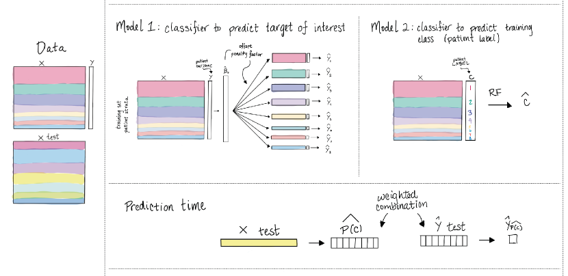
For simplicity assume that the target is binary, there are groups in the training set and (different) groups in the test set.
-
1.
Apply Algorithm 1 to yield individual models for each input group. Let the estimated probabilities Pr(Y=1|x) in group be .
-
2.
Fit a separate model to predict the training group from the features, using for example a random forest. Let be the resulting estimated class probabilities for for classes ,
-
3.
Given , the feature vector for a test observation, compute
(9) the estimated probability that for test group .
Although expression (9) makes sense mathematically, we have often found better empirical results if we instead train a supervised learning algorithm to predict from and .
4.4 Mass spectrometry cancer data
This data comes from a proteomics study of melanoma (Margulis et al., 2018). A total of 2094 peak heights from DESI mass spectometry were measured for each image pixel, with about a thousand pixels measured for each patient. There are 28 training patients, 15 test patients; a total of 29,107 training pixels, 20,607 test pixels. There is an average of about 1000 pixels per patient. The output target is binary (healthy vs disease). All error rates quoted are per pixel rates.
We clustered the training patients using K-means into 4 groups (see Table (2).
| Cluster | Members |
|---|---|
| 1 | 3 4 7 10 11 12 16 17 19 |
| 2 | 1 2 20 23 24 25 26 27 28 |
| 3 | 15 21 22 |
| 4 | 5 6 8 9 13 14 18 |
Tables 3, 4 and Figure 10 show the test error and AUC results. We see that the pretrained lasso provides a small advantage in AUC as compared to the overall model.
| Cluster | CV-AUC Pretrain | AUC Pretrain |
|---|---|---|
| 1 | 0.932 | 0.945 |
| 2 | 0.973 | 0.887 |
| 3 | 0.938 | 0.929 |
| 4 | 0.955 | 0.930 |
| Method | Test AUC |
|---|---|
| Overall model | 0.940 |
| Pretrained lasso using (9) | 0.935 |
| Pretrained lasso using supervised learner to predict | 0.960 |

Remark 6.
Pretrained lasso fits an interaction model. In general, suppose we have a target variable , features and grouping variables , As illustrated above, the grouping variables can stratify the inputs or the target (either multinomial or multi-response). Introduction of a grouping variable corresponds to the addition of an interaction term between and .
Thus one could imagine a more general forward stepwise pretraining process as follows:
-
1.
Start with an overall model, predicting from , without any consideration of the grouping variables. Let the and be the offset and penalty factor from the chosen model.
-
2.
Introduce the grouping variable by fitting individual models to the levels of , with the offset and penalty factor and . From these models extract and for the levels .
-
3.
Introduce the grouping variable , either as an interaction or an interaction , and so on.
Remark 7.
Input “grouping” with a continuous variable: Instead of a discrete grouping variable , suppose that we have a continuous modifying variable such as age. Here, we can use the pretrained lasso idea as follows:
-
1.
At the first stage, train a model using all rows of the , and without use of .
-
2.
At the second stage: fit a model again using all rows of , but now multiply each column, and the offset, by . Use the offset and penalty factor from the first model as defined in Section 2.3.
In the second stage, we force an interaction between age and the other features. This mirrors the case where the grouping variable is discrete; fitting separate models for each group is an interaction between the grouping variable and all other variables.
5 Learning the input groups
Here we consider the setting where there are no fixed input groups, but instead we learn potentially useful input groups from a CART tree. Typically, the features that we make available for splitting are not the full set of features but instead a small set of clinical variables that are meaningful to the scientist.
We illustrate this on the U.K. Biobank data, where we have derived 299 features on 64,722 white British individuals. There are 249 metabolites from nuclear magnetic resonance and 50 genomic PCs. We focus on myocardial infraction phenotype. The features available for splitting were age, PRS (polygenic risk score) and sex (0=female, 1=male).
We split the data into two equal parts at random (train/test) and built a CART tree using the R package rpart, limiting the depth of the tree to be 3 (for illustration). The left panel of Figure 11 shows the resulting tree. The right-most terminal node contains men with high PRS scores: their risk of MI is much higher than the other two groups (0.17 versus 0.027 and 0.05). The predictions using just this CART tree had a test AUC of 0.49.
We then applied the pretrained lasso for fixed input groups (Algorithm 1) to the three groups defined by the terminal nodes of the tree. The resulting tests AUC for the pretrained lasso and the overall model (an -regularized logistic regression) is shown in the right panel. We see that the pretrained lasso delivers about a 4-5% AUC advantage, for all values of .
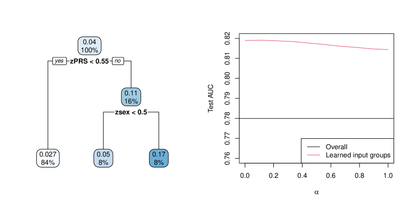
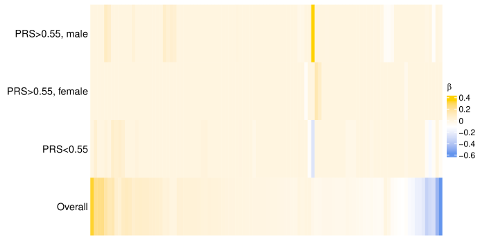
Figure 12 displays a heatmap of the non-zero coefficients within each of the three groups, and overall.
Another way to grow the a decision tree in this procedure would be to use “Oblique Decision Trees”, implemented in the ODRF R language package.222We thank Yu Liu and Yingcun Xia for implementing changes to their R package ODRF so that we could use it in our setting. These trees fit linear combinations the features at each split. Since the pretrained lasso fits a linear model (rather than a constant) in each terminal node, this seems natural here. We tried ODT in this example: it produced a very similar tree to that from CART, and hence we omit the details.
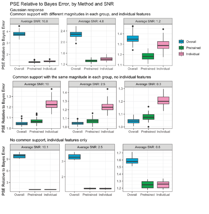
6 Simulation studies
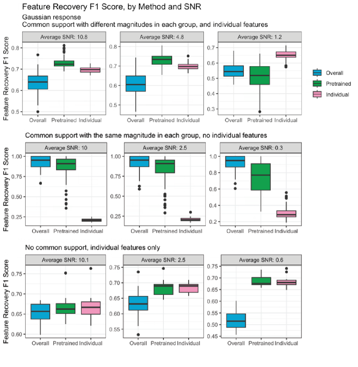
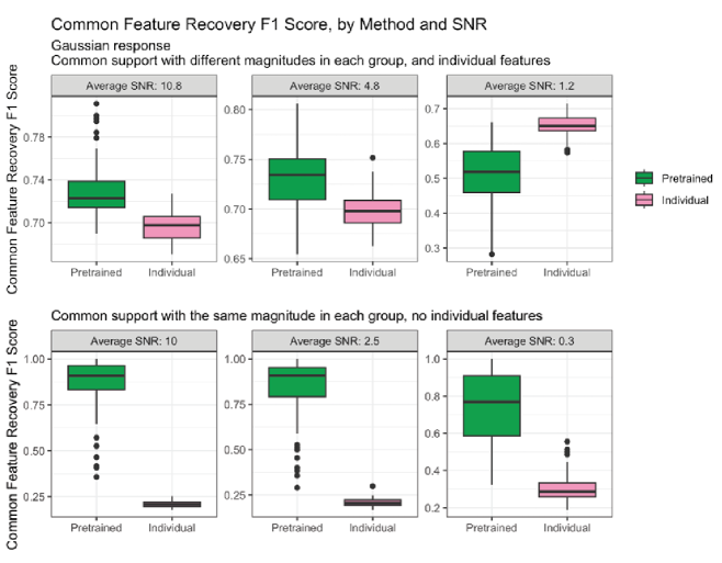
Here, we use simulations to compare pretraining with the overall model and individual models. The three approaches are compared in terms of (1) their predictive performance on test data and (2) their F1 scores for feature selection. Additionally, we compare pretraining to the individual models in terms of their ability to recover the common features; the features shared across all groups. Pretraining naturally identifies common features (using those identified in the first stage of training). For the individual model, we define common features as those which are selected for at least 51% of the group-specific models.
We focus here on data with a continuous response (Figures 13, 14 and 15) and five input groups (with observations each), across a range of signal-to-noise ratios (SNRs). In the first simulation, we create data with a common support and group-specific features, where the magnitude of the coefficients in the common support differs across groups. Then, we simulate data with a common support only (same magnitude), and finally we simulate data with individual features only. In the latter two cases, we expect the overall model and the individual models respectively to have the best performance. In general, we find that pretraining outperforms the overall and individual models when our assumptions are met: when there are features shared across all groups and features specific to each individual group. Further, pretraining has a particular advantage when the shared features have different magnitudes in each group.
We share the results from a more complete simulation study in Appendix A. There, the simulations cover three settings: grouped data with a continuous response (Table 5), grouped data with a binomial response (Table 6), and data with a multinomial response (Table 7).
7 Theoretical results on support recovery
In this section, we prove that the pretraining process recovers the true support and characterize the structure of the learned parameters under suitable assumptions on the training data.
7.1 Preliminaries
We call a random variable sub-Gaussian if it is centered, i.e., and
| (10) |
where is called the variance proxy of . For such a random variable, the following tail bound holds
| (11) |
We call that the random variable has bounded variance when its variance proxy is bounded by a constant. Examples of such random variables include the standard Gaussian and any random varible that is zero-mean and bounded by a constant.
7.2 An overview of the theoretical results
7.2.1 Conditions for deterministic designs
The recovery of the support of coefficients in lasso models is traditionally guaranteed by conditions like the irrepresentability condition. In this paper, we extend these conditions to the pretraining lasso. Specifically, we introduce a set of deterministic conditions that ensure the recovery of the true support in the shared support model, even when observations are mixed. These conditions, referred to as Pretraining Irrepresentability Conditions, are necessary and sufficient for the pretraining estimator to discard irrelevant variables and recover the true support. Although these conditions are slightly more complex than the classical irrepresentability condition due to the mixed observation model, they are easily interpretable. In summary, there are three key requirements: (1) the off-support features need to be incoherent with the features in the support, (2) the empirical covariance of the features in the support need to be well conditioned, (3) the individual parameters need to be bounded in magnitude.
7.2.2 Conditions for random designs
Two key aspects are studied when the design matrix is random:
-
•
Pretraining under isometric features: We introduce the subgroup isometry condition (18) to capture how representative the empirical covariance of a subgroup is in relation to the full dataset. This condition holds when the features are independent sub-Gaussian random variables, and helps in analyzing the behavior of the pretraining estimator.
-
•
Recovery under sub-Gaussian covariates: We prove in Theorems 1 and 2 that under certain conditions on the sample size, variable bounds, and noise levels, the pretraining estimator can recover the true support with high probability under the shared support model (12) where the supports are common. These results are similar in spirit to the existing recovery results for lasso (Wainwright, 2009), with a few crucial differences. In particular, it is known in the classical setting that measurements are necessary for support recovery with high probability. However, in our setting, our result given in Theorem 1 show that the number of measurements needs to scale as , where is an upper-bound on the magnitude of the weights . The extra factor is due to the mixture observation model (12) instead of a simple linear relation studied in earlier literature. It is an open question to verify that this factor is unavoidable, which we leave for future work.
In addition, we extend the shared support model (12) to lift the assumption that the supports are common, and consider the common and individual support model (23). In this model, there is a shared support between the groups, as well as additional individual supports. We show that support recovery results given in Theorems 1 and 2 still hold under the assumption that the magnitudes that belong to the individual support are sufficiently small for each . This is a necessary condition to ensure that the pretraining estimator only recovers the common support and discards individual supports for each group.
7.3 Shared support model
Consider sets of observations
| (12) |
where are unknown vectors which share a support of size . More precisely, we have where is the complement of the subset . Here, is a noise vector to account for the measurement errors, which are initially assumed to be deterministic. We assume that is an integer and each subgroup has at least samples, i.e., . We let to denote the full dataset and observations .
We define the pretraining estimator as
| (13) |
The individual models are defined as
| (14) |
for all . Here, we require an appropriate choice of the regularization weights .
7.3.1 Pretraining irrepresentability conditions
We now provide a set of deterministic conditions which guarantee that the pretraining estimator recovers the support of . Note that existing results on support recovery for lasso including the irrepresentability condition (Zhao & Yu, 2006), restricted isometry property (Van De Geer & Bühlmann, 2009) or random designs (Wainwright, 2009) are not applicable due to the mixed observation model in (12).
Recall that in the shared support model, the vectors have the same support of size . Let us use to denote the submatrix of the data matrix restricted to the support .
Lemma 1 (Pretraining irrepresentability).
Suppose that the conditions
| (15) | ||||
| (16) |
hold. Then, the pretraining estimator discards the complement of the true support , i.e., in the noiseless case, i.e., . In the noisy case, if the condition
| (17) |
holds, the same result holds for an arbitrary noise vector . Here, is the sign of the vectors constrained to their support S, and is the diagonal selector matrix for the -th set of samples, i.e., is padded with zeros.
7.3.2 Pretraining under isometric features
We now analyze the behaviour of the solution under the assumptions that the samples from the subgroups follow an isometric distribution relative to the entire dataset.
We introduce the subgroup isometry condition:
| (18) |
for some . The above quantity represents the ratio of empirical covariances of features restricted to the subset , comparing the entire dataset with the subgroup defined by the -th group of samples. It quantifies how representative the empirical covariance of the subgroup is in relation to the full dataset.
Remark 9.
Note that we have , where is the subset of samples that belong to the group and are features restricted to the true support .
Lemma 2.
Suppose that the samples are i.i.d. sub-Gaussian variables with bounded variance and let , where is a constant. Then, the subgroup isometry condition in (18) hold with probability at least , where and are constants.
Lemma 3.
Remark 10.
The above result shows that the pretraining estimator approximates the average of the individual models , in addition to a shrinkage term proportional to .
The above result is derived from the standard optimality conditions for the Lasso model, as detailed in Wainwright (2009) (see Appendix).
7.3.3 Recovery under random design
Next, we prove that the Pretraining Irrepresentability condition holds with high probability when the features are generated from a random ensemble.
Theorem 1.
Suppose that the samples are i.i.d. sub-Gaussian variables with bounded variance and the noise vectors are sub-Gaussian with variance proxy . In addition, assume that for some , and the number of samples satisfy
| (20) |
for some constant . Then, the conditions (15) and (16) when hold with probability at least where are constants. Therefore, discards the complement of the true support with the same probability.
Remark 11.
It is instructive to compare the condition (20) with the known results on recovery with lasso under the classical linear observation setting (Wainwright, 2009) that require observations. Therefore, using only the individual observations without pretraining, i.e., taking in (14), we need to achieve the same support recovery. Comparing this with Theorem 1, we observe that the pretraining procedure gives a factor improvement in the required sample size.
Remark 12.
We note that the factor is the extra cost on the number of samples induced by the mixture observation model, which is due to the second condition (16). In order the pretraining estimator to discard irrelevant variables, the magnitude of each linear model weight is required to be small. Furthermore, the pretraining estimator can discard variables from the true support .
Theorem 2.
Suppose that the samples are i.i.d. sub-Gaussian variables with bounded variance and the noise vectors are sub-Gaussian with variance proxy . Set . In addition, assume that for some , and the number of samples satisfy
| (21) |
and
| (22) |
for some constants . Then, the pretraining estimator exactly recovers the ground truth support with probability at least where are constants.
Remark 13.
Remark 14.
Note that there are pathological cases for which the pretraining estimator fails to recover the support. A simple example is where and . In this case, the condition (22) can not hold since . However, we are guaranteed that the pretraining estimator discards all the variables not in the ground truth support under the remaining assumptions.
7.4 Common and individual support model
We now consider sets of observations
| (23) |
where is an sparse vector to account for shared features and are sparse unknown vectors modeling individual features. We assume that the support of and are not-overlapping.
7.4.1 Recovery under random design
Next, we prove that the pretraining estimator discards the complement of the true support with high probability when the features are generated from a random ensemble and the magnitude of the individual coefficients are sufficiently small.
Theorem 3.
Suppose that the samples are i.i.d. sub-Gaussian variables with bounded variance and the noise vectors are sub-Gaussian with variance proxy . Set . In addition, assume that and for some and , and the number of samples satisfy
| (24) |
and
| (25) |
Then, the pretraining estimator exactly recovers the support of the common parameter with probability at least . Here, are constants.
Remark 15.
We note that the above theorem imposes the condition for some on the individual coefficients. This is a more stringent requirement compared to Theorem 1 where is unrestricted.
8 Multi-response models and chaining of the outcomes
Another interesting use-case is the multi-response setting, where the outcome has columns. The data in these columns may be quantitative or integers. The multinomial target discussed earlier can be expressed as a multi-response problem corresponding to one-hot encoding of the classes. But the multi-response setup is more general, and can be for example in problems where each observation can fall in more than one class.
To apply the pretrained lasso here, we simply fit a multi-response model (Gaussian or multinomial) to all of the columns, and then fit individual models to each of the columns separately.
Figure 16 shows an example taken from Skagerberg et al. (1992), simulating the production of low-density polyethylene. The data were generated to show that quality control could be performed using measurements taking during polyethylene production to predict properties of the final polymer. The authors simulated 56 samples with 22 features including temperature measurements and solvent flow-rate, and 6 outcomes: number-average molecular weight, weight-average molecular weight, frequency of short chain branching, the content of vinyl groups and vinylidene groups. Figure 16 shows the LOOCV squared error over the 6 outcomes, using both the best common (left plot) and the allowing to vary over the 6 outcomes. We see that pretrained lasso performs best in both settings.
Other multi-response settings include time-ordered target columns, and outcomes of different types (e.g. quantitative, survival, binary). In both cases we can apply pretrained lasso in a sequential (chained) fashion. We fit a model to the first outcome, compute the offset and penalty factor, and pass these to a model which fits to the second outcome, and so on.
We illustrate the second scenario in Figure 17. We generated three outcome variables— quantitative, censored survival and binary— all functions of a (sparse) linear predictor . The and noise levels were chosen so that the Gaussian linear model (for the first outcome) had an SNR of about 2. The figure panels show the test set results (in green) for the survival outcome and the binary outcome, as a function of the pretraining hyperparameter . For comparison, the test set C-index and AUC for the survival and binary outcomes, modelled separately, are shown in red. We see that the pretrained lasso is able to borrow strength from one target to the next, and as a result, yields higher accuracy.
This application of pretrained lasso to mixed outcomes requires a prior ordering of the outcomes. In real applications it might make sense to place the primary outcome measure in the first position, and the rest in decreasing order of importance.

9 Conditional average treatment effect (CATE) estimation
An important problem in causal inference is the estimation of conditional average treatment effects. In the most common setting, the data is of the form where is a vector of covariates, is a quantitative outcome and is a binary treatment indicator. We denote by the corresponding outcomes we would have observed given the treatment assignment or 1 respectively. The goal is to estimate the CATE . We make the usual assumption that the treatment assignment is unconfounded.
One popular approach is the “R-learner” of Nie & Wager (2021). It is based on the objective function
| (26) |
where is the overall mean function and is the treatment propensity . In the simplest case (which we focus on here), a linear model is used for and . The lasso version of the R-learner adds an penalty to the objective function.
The steps of the R-learner are as follows:
-
1.
Estimate by fitting on , on , using cross-fitting
-
2.
Estimate by solving (26) above
For simplicity we assume here that the treatment is randomized so that we can set .
Now we can combine the R-learner with the pretrained lasso as follows: We assume the shared support model
| (27) | |||||
| (28) |
where has the same support and signs as . To fit this, we use the same R-learner procedure above, but include in the model for the penalty factor computed from the model for [we do not include the offset, since the target in the two models are different]. If this shared support assumption is true or approximately true, we can potentially do a better job at estimating . This assumption also seems reasonable: it says that the predictive features are likely to overlap with the features that modify the treatment effect.
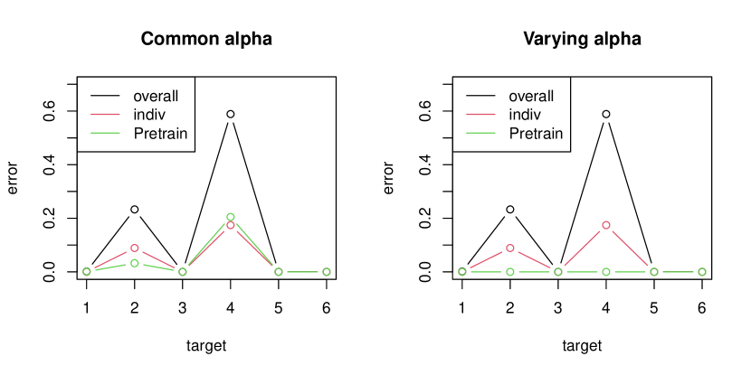
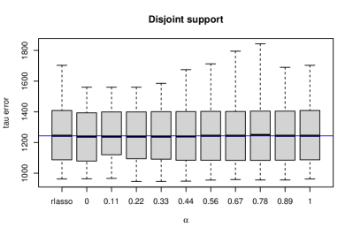
Figure 18 shows an example with and an SNR of about 2. The first 10 components of are positive, while the second 10 components are zero. In left panel the treatment effect has the same support and positive signs as , while in the right panel, its support is in the second 10 features, with no overlap with the support of . The figure shows boxplots of the absolute estimation error in over 20 realizations.
In the left panel we see that for all values of the pretrained R-learner outperforms the R-learner, while in the right panel, they behave very similarly. It seems that there is little downside in assuming the shared support model. Upon closer examination, the reason becomes clear: under Model 28 with disjoint support, all 20 features are predictive of the outcome, and hence there is no support restriction resulting from the fit of the outcome model.
10 Beyond linear models: an application to gradient boosting
Here we explore the use of basis functions beyond the linear functions used throughout the paper. Suppose we run gradient boosting (Chen & Guestrin, 2016) for steps, giving trees. Then we can consider the evaluated trees as our new variables, yielding a new set of features. We then apply the pretrained lasso to these new features. Here is the procedure in a little more detail:
-
•
run iterations of xgboost to get trees (basis functions) ()
-
•
run the pretrained lasso on .
Consider this procedure in the fixed input groupings use-case. We use the lasso to estimate optimal weights for each of the trees, both for an overall model, and for individual group models. For the usual lasso, this kind of “post-fitting” is not new (see e.g. RuleFit (Friedman & Popescu, 2008) and ESL (Hastie et al., 2009) page 622).
It is easy to implement this procedure using the xgboost library in R (Chen et al., 2023). Figure 19 shows the results from a simulated example. We first used xgboost to generate 50 trees of depth 1 (stumps). Then we simulated data using these trees as features, with a strong common weight vector .
The test error results are shown in Figure 19. The first method— xgboost— is vanilla boosting applied to the raw features, while the other three methods use the 50 initial trees generated by xgboost.

We see that lasso pretraining can help boosting as well.
11 Does cross-validation work here?
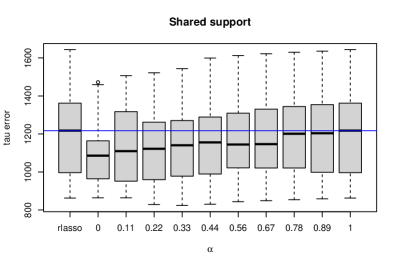
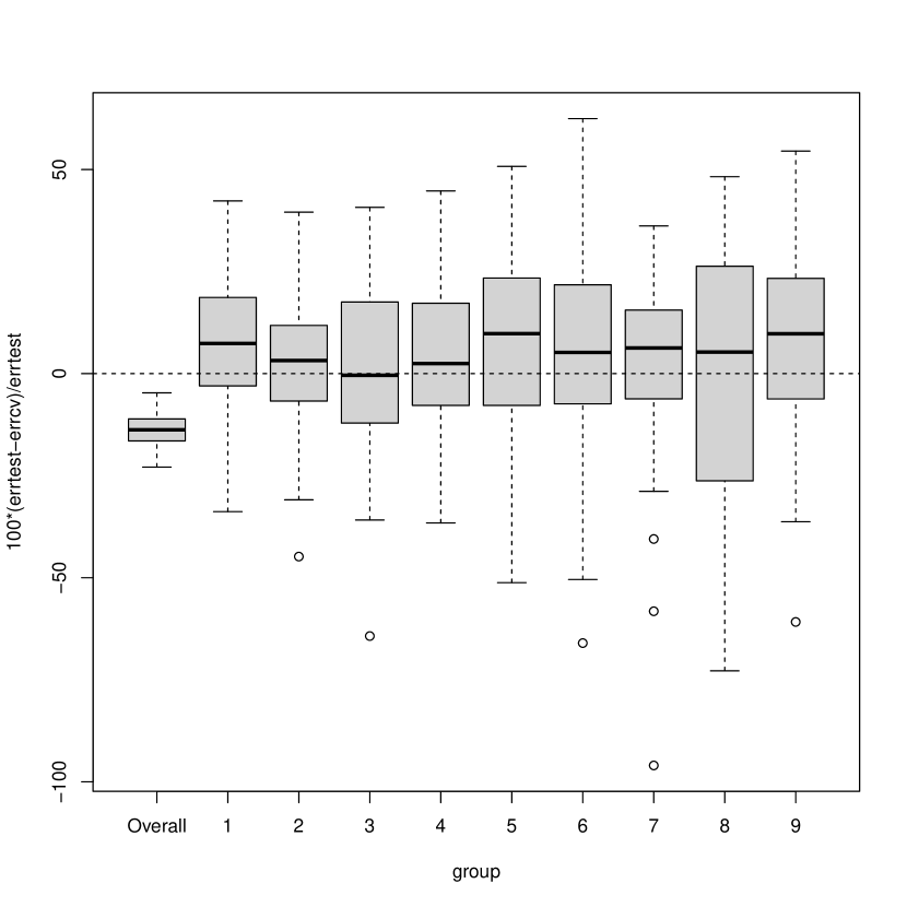
In lasso pretraining, “final” cross-validated error that we use for the estimation of both and is the error reported in the last application of cv.glmnet. There are many reasons why this estimate might be biased for the test-error. As with usual cross-validation with folds, each training set has observations (rather than and hence the CV estimate will be biased upwards. On the other hand, in the pretrained lasso, we re-used the data in the applications of cv.glmnet, and this should cause a downward bias. Note that we could instead do proper cross-validation— leaving out data and running the entire pipeline for each fold. But this would be prohibitively slow.
We ran a simulation experiment to examine this bias. The model was the same as that used in Figure 5, with the results in Figure 20. The y-axis shows the relative error in the CV estimate as a function of the true test error. The boxplot on the left corresponds to the overall model fit via the lasso: as expected, the estimate is a little biased upwards. The other boxplots show that the final reported CV error is on the order of 5 or 10% too small as an estimate of the test error, Hence this bias does not seem like a major practical problem, but should be kept in mind.
12 Discussion
In this paper we have developed a framework that enables the power of ML pretraining — designed for neural nets — to be applied in a simpler statistical setting (the lasso). We discuss many diverse applications of this paradigm, including stratified models, multinomial targets, multi-response models, conditional average treatment estimation and gradient boosting. There are likely to be other interesting applications of these ideas, including the transfer of knowledge from a model pretrained on a large corpus, and then fine-tuned on a smaller dataset for the task at hand.
We plan to release an open source R language package that implements these ideas.
Acknowledgements
The authors would like to thank Emmanuel Candes, Daisy Ding, Trevor Hastie, Sarah McGough, Vishnu Shankar, Lu Tian, Ryan Tibshirani, and Stefan Wager for helpful discussions. We thank Yu Liu and Yingcun Xia for implementing changes to their R package ODRF. B.N. was supported by National Center For Advancing Translational Sciences of the National Institutes of Health under Award Number UL1TR003142. M.A.R. is in part supported by National Human Genome Research Institute (NHGRI) under award R01HG010140, and by the National Institutes of Mental Health (NIMH) under award R01MH124244 both of the National Institutes of Health (NIH). R.T. was supported by the National Institutes of Health(5R01EB001988-16) and the National Science Foundation(19DMS1208164). M.P. was supported in part by the National Science Foundation (NSF) under Grant DMS-2134248, in part by the NSF CAREER Award under Grant CCF-2236829, in part by the U.S. Army Research Office Early Career Award under Grant W911NF-21-1-0242, and in part by the Stanford Precourt Institute. E.C. was supported by the Stanford Data Science Scholars Program and the Stanford Graduate Fellowship. J.S. was supported by the National Institute of General Medical Sciences grant R35 GM139517, Stanford University Discovery Innovation Award, and the Chan Zuckerberg Data Insights.
Appendix A Simulation study results
Here we include more complete results of the simulation study described in Section 6. As before, we compare pretraining with the overall model and individual models in terms of (1) predictive performance on test data, (2) their F1 scores for feature selection and (3) F1 scores for feature selection among the common features only. Our simulations cover grouped data with a continuous response (Table 5), grouped data with a binomial response (Table 6), and data with a multinomial response (Table 7).
| SNR | PSE relative to Bayes error | Feature F1 score | Common feature F1 score | |||||
| Overall | Pretrain | Indiv. | Overall | Pretrain | Indiv. | Pretrain | Indiv. | |
| Common support with same magnitude, individual features | ||||||||
| Features: common, per group, total | ||||||||
| As above, but now | ||||||||
| Features: common, per group, total | ||||||||
| Common support with same magnitude, no individual features | ||||||||
| Features: common, per group, total | ||||||||
| Common support with different magnitudes, no individual features | ||||||||
| Features: common, per group, total | ||||||||
| As above, but now with individual features | ||||||||
| Features: common, per group, total | ||||||||
| Individual features only | ||||||||
| Features: common, per group, total | ||||||||
| — | — | |||||||
| — | — | |||||||
| — | — | |||||||
| Test AUC | Feature F1 score | Common feature F1 score | ||||||
| Bayes | Overall | Pretrain | Indiv. | Overall | Pretrain | Indiv. | Pretrain | Indiv. |
| Common support with same magnitude, individual features | ||||||||
| Features: 5 common, 5 per group, 40 total | ||||||||
| As above, but now | ||||||||
| Features: 5 common, 5 per group, 320 total | ||||||||
| Common support with same magnitude, no individual features | ||||||||
| Features: 5 common, 0 per group, 40 total | ||||||||
| Common support with different magnitudes, no individual features | ||||||||
| Features: 5 common, 0 per group, 40 total | ||||||||
| As above, but now with individual features | ||||||||
| Features: 5 common, 5 per group, 40 total | ||||||||
| Individual features only | ||||||||
| — | — | |||||||
| — | — | |||||||
| — | — | |||||||
| Test misclass. rate | Feature F1 score | Common feature F1 score | ||||||
| Bayes rule | Overall | Pretrain | Indiv. | Overall | Pretrain | Indiv. | Pretrain | Indiv. |
| Common support, individual features | ||||||||
| Features: 3 common, 10 per group, 159 total | ||||||||
| As above, but now | ||||||||
| Features: 3 common, 10 per group, 640 total | ||||||||
| Common support, no individual features | ||||||||
| Features: 3 common, 0 per group, 159 total | ||||||||
| Individual features only | ||||||||
| Features: 0 common, 10 per group, 159 total | ||||||||
| — | — | |||||||
| — | — | |||||||
Appendix B Mathematical Proofs
B.1 Proof of Lemma 1
We analyze the conditions for optimality of the pretraining estimator given in (13). We apply the scaling and to absorb the factor and simplify our notation. Suppose that the support of the optimal solution is , which is assumed to contain the support of . The optimality conditions that ensure is the unique solution with support are as follows
| (29) | ||||
| (30) |
where is the optimal solution. When the matrix is full column-rank, the matrix is invertible and we can solve for as follows
| (31) |
Plugging in the observation model , we obtain
| (32) |
Plugging in the above expression into the condition (30), and dividing both sides by , we obtain
| (33) |
Using triangle inequality, we upper-bound the left-hand-side to arrive the sufficient condition
| (34) |
Therefore by imposing the conditions
| (35) | ||||
| (36) | ||||
| (37) |
we observe that the optimality conditions for with the support are satisfied.
B.2 Proof of Theorem 1
First condition
We consider the first condition of pretraining irrepresentability given by
| (38) |
Note that and are independent for . Therefore, is sub-Gaussian with variance proportional to .
When for some constant , the matrix is a near-isometry in spectral norm, i.e.,
| (39) |
with probability at least where are constants. Therefore for , we have and .
Applying union bound, we obtain
| (40) | ||||
| (41) | ||||
| (42) |
for some constant .
Consequently, for we have with probability at least where are constants.
Second condition
We proceed bounding the second irrepresentability condition involving the matrix using the same strategy used above.
Note the critical fact that the shared support model implies the matrices and
are independent since the latter matrix only depends on the features .
Note that
| (43) | ||||
| (44) |
Recalling the scaling of the by , we note that is an formed by the concatenation of an an matrix of i.i.d. sub-Gaussian variables with variance with an matrix of zeros. From standard results on the singular values of sub-Gaussian matrices Vershynin (2018), we have with probability at least . Using the fact that has entries bounded in , we obtain the upper-bound
| (45) | ||||
| (46) | ||||
| (47) | ||||
| (48) | ||||
| (49) |
where we used , i.e., each subgroup has at least samples, in the final inequality. Repeating the same sub-Gaussianity argument and union bound used for the first condition above, we obtain that for we have with probability at least where are constants.
Third condition
Using standard results on Gaussian vectors, and repeating the union bound argument used in analyzing the first condition, we obtain that when we set and with probability at least where are constants.
Applying union bound to bound the probability that all of the three conditions hold simultaneously, we complete the proof of the theorem.
B.3 Proof of Lemma 2
We apply well-known concentration bounds for the extreme singular values of i.i.d. Gaussian matrices (see e.g. Vershynin (2018)). These bounds and for each fixed with high probability when . Applying union bound over , we obtain the claimed result.
B.4 Proof of Lemma 3
B.5 Proof of Theorem 2
Note that we only need to control the signs of given in (31), in addition to the guarantees of Theorem 1. Our strategy is to bound the norm of via its norm and establishing entrywise control on by the assumption on the minimum value of the average . We combine Lemma 2 and Lemma 3 with the expression to obtain
| (50) |
with high probability. Noting that with high probability, and by our assumption on the magnitude of , we obtain the claimed result.
B.6 Proof of Theorem 3
The main difference of this result compared to the proof of Theorem 1 is in the analysis of the quantity . Unfortunately, and are no longer independent. We proceed as follows
| (51) | ||||
| (52) | ||||
| (53) |
we bound the last term via and impose . Note that with high probability due to the rescaling by . The rest of the proof is identical to the proof of Theorem 1.
References
- (1)
-
Chaung et al. (2023)
Chaung, K., Baharav, T. Z., Henderson, G., Zheludev, I. N., Wang, P. L.
& Salzman, J. (2023), ‘Splash: A
statistical, reference-free genomic algorithm unifies biological discovery’,
Cell 186(25), 5440–5456.e26.
https://www.sciencedirect.com/science/article/pii/S0092867423011790 - Chen & Guestrin (2016) Chen, T. & Guestrin, C. (2016), Xgboost: A scalable tree boosting system, in ‘Proceedings of the 22nd acm sigkdd international conference on knowledge discovery and data mining’, pp. 785–794.
-
Chen et al. (2023)
Chen, T., He, T., Benesty, M., Khotilovich, V., Tang, Y., Cho, H., Chen, K.,
Mitchell, R., Cano, I., Zhou, T., Li, M., Xie, J., Lin, M., Geng, Y., Li, Y.
& Yuan, J. (2023), xgboost:
Extreme Gradient Boosting.
R package version 1.7.6.1.
https://CRAN.R-project.org/package=xgboost - Consortium et al. (2022) Consortium, T. T. S., Jones, R. C., Karkanias, J., Krasnow, M. A., Pisco, A. O., Quake, S. R., Salzman, J., Yosef, N., Bulthaup, B., Brown, P. et al. (2022), ‘The tabula sapiens: A multiple-organ, single-cell transcriptomic atlas of humans’, Science 376(6594), eabl4896.
- Friedman & Popescu (2008) Friedman, J. H. & Popescu, B. E. (2008), ‘Predictive learning via rule ensembles’.
- Friedman et al. (2010) Friedman, J., Tibshirani, R. & Hastie, T. (2010), ‘Regularization paths for generalized linear models via coordinate descent’, Journal of Statistical Software 33(1), 1–22.
- Goldman et al. (2020) Goldman, M. J., Craft, B., Hastie, M., Repečka, K., McDade, F., Kamath, A., Banerjee, A., Luo, Y., Rogers, D., Brooks, A. N. et al. (2020), ‘Visualizing and interpreting cancer genomics data via the xena platform’, Nature biotechnology 38(6), 675–678.
- Gross & Tibshirani (2016) Gross, S. M. & Tibshirani, R. (2016), ‘Data shared lasso: A novel tool to discover uplift’, Computational statistics & data analysis 101, 226–235.
- Hastie et al. (2009) Hastie, T., Tibshirani, R., Friedman, J. H. & Friedman, J. H. (2009), The elements of statistical learning: data mining, inference, and prediction, Vol. 2, Springer.
- Kokot et al. (2023) Kokot, M., Dehghannasiri, R., Baharav, T., Salzman, J. & Deorowicz, S. (2023), ‘Splash2 provides ultra-efficient, scalable, and unsupervised discovery on raw sequencing reads’, BioRxiv .
- Margulis et al. (2018) Margulis, K., Chiou, A. S., Aasi, S. Z., Tibshirani, R. J., Tang, J. Y. & Zare, R. N. (2018), ‘Distinguishing malignant from benign microscopic skin lesions using desorption electrospray ionization mass spectrometry imaging’, Proceedings of the National Academy of Sciences 115(25), 6347–6352.
-
McGough et al. (2023)
McGough, S. F., Lyalina, S., Incerti, D., Huang, Y., Tyanova, S., Mace, K.,
Harbron, C., Copping, R., Narasimhan, B. & Tibshirani, R.
(2023), ‘Prognostic pan-cancer and
single-cancer models: A large-scale analysis using a real-world
clinico-genomic database’, medRxiv .
https://www.medrxiv.org/content/early/2023/12/19/2023.12.18.23300166 - Nie & Wager (2021) Nie, X. & Wager, S. (2021), ‘Quasi-oracle estimation of heterogeneous treatment effects’, Biometrika 108(2), 299–319.
- Olivieri et al. (2021) Olivieri, J. E., Dehghannasiri, R., Wang, P. L., Jang, S., De Morree, A., Tan, S. Y., Ming, J., Wu, A. R., Quake, S. R., Krasnow, M. A. et al. (2021), ‘Rna splicing programs define tissue compartments and cell types at single-cell resolution’, Elife 10, e70692.
- Schilder et al. (2012) Schilder, R. J., Kimball, S. R. & Jefferson, L. S. (2012), ‘Cell-autonomous regulation of fast troponin t pre-mrna alternative splicing in response to mechanical stretch’, American Journal of Physiology-Cell Physiology 303(3), C298–C307.
- Skagerberg et al. (1992) Skagerberg, B., MacGregor, J. F. & Kiparissides, C. (1992), ‘Multivariate data analysis applied to low-density polyethylene reactors’, Chemometrics and intelligent laboratory systems 14(1-3), 341–356.
- Tuck & Boyd (2021) Tuck, J. & Boyd, S. (2021), ‘Fitting laplacian regularized stratified gaussian models’, Optimization and Engineering pp. 1–21.
- Van De Geer & Bühlmann (2009) Van De Geer, S. A. & Bühlmann, P. (2009), ‘On the conditions used to prove oracle results for the lasso’.
- Vershynin (2018) Vershynin, R. (2018), High-dimensional probability: An introduction with applications in data science, Vol. 47, Cambridge university press.
- Wainwright (2009) Wainwright, M. J. (2009), ‘Sharp thresholds for high-dimensional and noisy sparsity recovery using l1-constrained quadratic programming (lasso)’, IEEE transactions on information theory 55(5), 2183–2202.
- Yu et al. (2019) Yu, G., Bien, J. & Tibshirani, R. (2019), ‘Reluctant interaction modeling’, arXiv preprint arXiv:1907.08414 .
- Zhao & Yu (2006) Zhao, P. & Yu, B. (2006), ‘On model selection consistency of lasso’, The Journal of Machine Learning Research 7, 2541–2563.