Propagation reversal on trees in the large diffusion regime
Hermen Jan Hupkes
hhupkes@math.leidenuniv.nlMathematisch Instituut, Universiteit Leiden, P.O. Box 9512, 2300 RA Leiden, The NetherlandsMia Jukić
mia.jukic@tno.nlMathematisch Instituut, Universiteit Leiden, P.O. Box 9512, 2300 RA Leiden, The NetherlandsElectromagnetic Signatures & Propagation, Netherlands Organisation for Applied Scientific Research (TNO), 2509 JG The Hague, The Netherlands
Abstract
In this work we study travelling wave solutions to bistable reaction diffusion equations on bi-infinite -ary trees in
the continuum regime where the diffusion parameter is large.
Adapting the spectral convergence method developed by Bates and his coworkers,
we find an asymptotic prediction for the speed of
travelling front solutions. In addition, we prove that
the associated profiles converge to the solutions of
a suitable limiting reaction-diffusion PDE. Finally,
for the standard cubic nonlinearity we provide explicit formula’s
to bound the thin region in parameter space where
the propagation direction undergoes a reversal.
In this work we study the reaction-diffusion-advection lattice differential equation (LDE)
(1.1)
As explained below, we view the (real-valued) parameter as a branching factor. In addition, encodes the diffusion strength and the nonlinearity is of bistable type, for example
(1.2)
This LDE is known [13] to admit travelling front solutions, i.e. solutions
of the form
(1.3)
In this paper we apply a version of the ‘spectral convergence’ technique
to study the behaviour of the pair in the regime
where is large, the so-called continuum regime. In particular, our results supplement our earlier work [9],
where we studied the small and intermediate regime using an
entirely different set of techniques.
Dynamics on -ary trees
Our primary motivation to study (1.1) is that
the wavefronts (1.3) can be seen as
layer-wave solutions of bistable reaction-diffusion equations posed on -ary trees. In particular, the sign of the wavespeed determines which of the two stable roots of the nonlinearity can be expected to spread throughout the tree. We refer the reader to our previous work [9] and a prior paper by Kouvaris, Kori and Mikhailov [11] for numerical studies to support this claim and and an in-depth discussion of the potential application areas for our results.
Related results for monostable equations can be found in [8]. Preliminary numerical investigations
show that for general trees, studying (1.1)
with the average branch-factor still has important
predictive capabilities.
For each fixed , the main results in [9]
provide non-empty open sets of parameters where the expressions
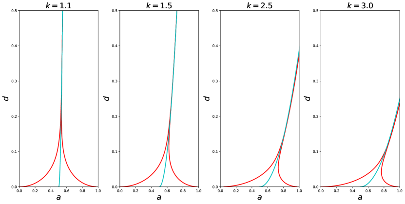
, respectively are guaranteed to hold. In fact, upon steadily increasing the diffusion parameter for a fixed , waves transition from being pinned , travelling ‘down’ the tree , being pinned once more
towards finally travelling ‘up’ the tree . This is illustrated
by the numerical results in Fig. 1.
These results were achieved by constructing explicit sub- and super-solutions and invoking the comparison principle. Although the boundaries of these regions agree reasonably well with numerical observations for small ,
they are - by construction - not ‘asymptotically precise’. In particular, they do not accurately capture the transition region between and , which appears to converge to a curve as increases. The main purpose of our results here is to increase our understanding of this transition
region where propagation reversal occurs.
Continuum regime
In order to gain some preliminary intuition into the
diffusion-driven propagation reversal discussed above,
we recall from [9] that
the LDE (1.1) can also
be interpreted as a spatial discretization of the
partial differential equation (PDE)
(1.4)
Indeed, using the correspondence
and the relation
(1.5)
the standard central difference schemes
(1.6)
reduce (1.4) back to (1.1). Vice-versa, expanding the shifted terms in (1.1) up to order
leads directly to (1.4).
For the cubic (1.2), the PDE (1.4) admits explicit travelling front solutions
(1.7)
Upon introducing the appropriate speed-scaling
and recalling the coefficients (1.5),
we readily obtain the asymptotic prediction
(1.8)
which changes sign at the critical value
(1.9)
The numerical results in Figure 1 illustrate
that this prediction retains its accuracy for intermediate values of , corresponding to values of that are far removed from the critical
regime .
Spectral convergence
Our main results provide a rigorous interpretation
and quantification for asymptotic predictions of this type.
This is achieved by using the spectral convergence approach
that was pioneered by Bates and his coworkers in
[5]. The main
feature of this approach is that
Fredholm properties of
linearized operators associated to travelling wave solutions
can be transferred from the spatially continuous setting of
(1.4) to the spatially discrete
setting of (1.1).
The latter operators can then be used
in a standard fashion to close a fixed-point argument
and construct travelling front solutions to (1.1)
that are close to those of their PDE counterpart
(1.4).
The main difficulty that needs to be overcome is that
this perturbation is highly singular, since (unbounded) derivatives
are replaced by difference quotients. As a consequence,
one must carefully work with weak limits
and use spectral properties of the (discrete) Laplacian together with
the bistable structure of the nonlinearity
to counteract the loss of information that typically occurs
when using the weak topology.
In the present paper, the main additional complication
is the extra convective term appearing in the limiting
PDE (1.4) for . Indeed,
the coefficients
introduced in (1.5) scale differently
with respect to . In particular, in our analysis
the associated extra terms cannot be seen as ‘small’
and must be handled with care by invoking the
natural directional asymmetry that trees have.
A second main issue is that we want to obtain estimates
that are uniform in terms of the parameters and .
Such control is necessary in order to formulate quantitative results
for the critical curves .
Outlook
Let us emphasize that we expect that our techniques
can be applied to a much larger class of problems
than the scalar setting of (1.1).
For example, following the framework developed in [16],
it should be possible to perform a similar analysis
for the FitzHugh-Nagumo system
and other multi-component reaction-diffusion problems.
Indeed, we do not use the comparison principle in this paper,
as opposed to the earlier work in [9].
We also note that the results in [5] are actually strong enough to
handle discretizations of the Laplacian that have infinite range
interactions. In particular, our analysis here should also be applicable
for (regular) dense graphs. We also envision possible extensions to irregularly structured sparse graphs through the use of the recently developed theory of graphops [3, 12].
It is well-known that travelling waves can be used as building blocks to uncover and describe more complex dynamics occurring in spatially extended systems [2]. We therefore view the current paper as part of a push towards understanding and uncovering the behaviour of systems
in spatially structured environments, which can often naturally be modelled using graphs [1, 18, 19, 21]. The ability to incorporate such spatial structures into models is becoming more and more important in our increasingly networked world.
Indeed, dynamical systems on networks are being
used in an ever-increasing range of disciplines, including chemical reaction theory [6],
neuroscience [20], systems biology [14],
social science [17], epidemiology [4]
and transportation
networks [15].
Organization
We state our assumptions and main results in §2
and discuss the general strategy towards solving the
associated fixed point in §3. The relevant linear
theory is developed in §4, while the required nonlinear
estimates are obtained in §5.
Acknowledgments
Both authors acknowledge support from the Netherlands Organization for Scientific Research (NWO) (grant 639.032.612).
Figure 1: The red curves denote the numerically computed boundaries of the pinning region where . The cyan
curves originating from represent
the asymptotic prediction (1.9), which retains its accuracy even for relatively large values of the branching factor .
2 Main results
In order to state our main result for (1.1),
we first formalize the bistability condition that we impose
on the nonlinearity .
(Hg)
The map is -smooth on and
for all we have the identities
together with the inequalities
and the sign conditions
Fixing and turning to travelling waves, it turns out to be convenient to link the diffusion strength to a new grid-size parameter
via the (invertible) relations
(2.1)
which reduce to in the symmetric case .
To appreciate this, we recall the standard central difference schemes
(1.6)
and introduce the associated operators
we find that the (rescaled) profile
must satisfy the mixed-type functional differential equation (MFDE)
(2.4)
with ,
to which we couple the standard spatial limits
(2.5)
On the one hand, this MFDE is covered by the general framework developed by Mallet-Paret in [13]. This provides the solutions
that lie at the basis of our analysis in this paper.
Proposition 2.1.
[13, Thm. 2.1]
Suppose that (Hg) holds and pick
together with and .
Then there exist a speed and a non-decreasing profile that satisfy (2.4) with ,
together with the boundary conditions (2.5).
Moreover, is uniquely determined and depends -smoothly on all parameters when . In this case the profile is -smooth with and unique up to translation.
On the other hand, under the convergence assumption
(2.6)
one may readily take
the formal limit of (2.4)
to arrive at the ODE
(2.7)
A classic result (see e.g. [7]) states that
there is a unique wavespeed for which
(2.7) with the boundary conditions
(2.5) admits a solution . This waveprofile is unique up to translation and has .
The goal of this paper is to link these two viewpoints together from
a spectral convergence perspective, extending earlier
work in [5] that applies to the case.
The presence of the discrete derivative
in (2.4) with a
coefficient of size introduces complications.
In fact, our approach can only keep this (large) term under control
if it satisfies a sign condition, which we will achieve
by exploiting the
asymmetry that the parameter introduces into our problem.
In particular, we need to restrict the values of the detuning parameter
by requiring positive values for the continuum wave speed .
To this end, we introduce the set
(2.8)
noting that the second characterization can be obtained by integrating (2.7) against . With this notation in place,
we are ready to state our main result.
Assume that holds and pick a compact subset . Then there exist constants
and so that for any , any
and any
we have the bound
(2.9)
In order to illustrate the application range of this theorem and highlight the uniformity of
the estimates, we return to the setting of the cubic nonlinearity (1.2).
In this case we have
(2.10)
and we recall the critical curve
(2.11)
discussed in §1.
Applying the bound (2.9)
with as given in (2.1), we immediately find
(2.12)
Our final result formulates a number of such estimates directly in
terms of this critical curve . In particular, we capture the
transition between waves that propagate up the tree
and down the tree. For explicitness,
we have absorbed all unknown constants into a single upper bound
for the branch factor. The price is that the exponent
appearing in the correction curves is not optimal; it can
be increased up to (but not including) .
Corollary 2.3.
Let be the standard cubic nonlinearity (1.2) and
pick . Then there exists
so that the following properties hold
for all
and .
(i)
We have the bound
(2.13)
(ii)
We have whenever
(2.14)
(iii)
We have whenever
(2.15)
Proof.
We write
and recall the constants and defined in
Theorem 2.2. In addition, we write
(2.16)
for the implicitly predicted wavespeed appearing
in (2.9). In order to exploit
these upper and lower bounds,
we pick , write and set out to solve
(2.17)
Upon introducing the expressions
(2.18)
the quadratic formula formally yields the two solutions
By further restricting we can ensure that and that (2.12)
can be simplified to (2.13), which
completes the proof.
∎
3 Fixed point problem
In this section we setup the fixed point problem that
will enable us to extract the bounds (2.9).
In particular, we isolate the correct linear and nonlinear parts
and formulate a convergence result for the associated linear operators.
The overall strategy closely resembles the approach originally developed in [5] and generalized
in [10, 16].
In order to extract the anticipated speed correction
(2.6), we recall
the discrete derivatives (2.2)
and introduce the combined operator
(3.1)
This allows us to recast the MFDE (2.4)
in the form
(3.2)
We now consider the pair as a perturbation
from the profile and the
anticipated wavespeed (2.6)
by writing
(3.3)
A direct computation shows that solving (3.2) is equivalent to finding a solution to the problem
(3.4)
where we have introduced the two nonlinearities
(3.5)
together with the linear operator
(3.6)
The key point is that the nonlocal operator formally converges to the well-known second order differential operator that acts as
Our first main contribution is the analogue of [10, Thm. 2.3] for the current setting and shows
in a sense that the characterization (3.8) can be transferred to the operators .
Consider the setting of Theorem 2.2. Then there exists
and such that for all , and , the fixed point problem
(3.16) posed on the set with
has a unique solution .
The result follows directly from Proposition 3.2 and the identifications (3.3).
∎
4 Linear theory
Our goal in this section is to establish Proposition 3.1, modifying
the approach in [5] to
account for the term present in the operator
defined in (3.1). As a preparation,
we introduce the formal adjoints
(4.1)
together with
(4.2)
Our key task is to establish lower bounds for the quantities
(4.3)
as stated in the following result,
which is analogous to [5, Lem. 6].
Proposition 4.1.
Suppose that (Hg) is satisfied and pick
a compact set .
Then there exists and
such that for every
we have
(4.4)
Indeed, for small these lower bounds readily allow us to extend
the estimate
(4.5)
that is available for the limiting second-order differential operator
(3.7); see e.g. [5, Lem. 5].
We remark that the constant in (4.5) can be chosen uniformly
with regards to the parameter in compact subsets of on account of the smoothness of .
This extension result should be compared
to [5, Thm. 4] and can be used
to establish Proposition 3.1
by following the procedure in [10].
Corollary 4.2.
Suppose that (Hg) is satisfied and pick a
compact set .
There exists constants and
together with a map
so that the following holds true.
For any ,
any , any and any , the operator
is invertible as a map
from onto and satisfies the bound
(4.6)
Proof.
Following the proof of
[5, Thm. 4],
we fix and a
sufficiently small . We subsequently pick
an arbitrary and .
By Proposition 4.1,
the operator is an homeomorphism
from onto its range
(4.7)
with a bounded inverse . The latter fact
shows that is a closed subset of .
If , there exists a non-zero
so that ,
i.e.,
(4.8)
Restricting this identity to test functions
implies that in fact .
In particular, we find
(4.9)
which by the density of in means that .
Applying Proposition 4.1 once more
yields the contradiction
and establishes .
The bound (4.6)
with the constant that does not depend on the parameters
now follows directly from the definition (4.3) of the
quantities
and the uniform lower bound (4.4).
∎
Setting out to find lower bounds for the quantities
(4.3),
we first provide some basic properties of the operator .
An important difference with [5, Lem. 3] is
that the estimate (4.13)
only provides inequalities instead of the equalities that are possible for .
Lemma 4.3.
Consider a function , write
(4.10)
and suppose that . Then
for any and
we have the bound
(4.11)
In addition, the inequalities
(4.12)
hold for any , and .
If in fact , then we also have the inequalities
(4.13)
Proof.
In view of the uniform bound for ,
the estimate (4.11) follows
directly from a Taylor expansion. Turning to
the remaining inequalities,
we note that the Fourier symbol associated to is given by
(4.14)
In particular, the functions
(4.15)
are both even and non-positive, from which the claims follow
readily.
∎
The next step is to show that
the limiting
values in (4.4)
can be approached
via a sequence of realizations
that convergence in an appropriate
weak sense. The key point is that weak limits
can also be extracted from the operators
when considered on appropriate sequences in ;
see (4.22).
Lemma 4.4.
Consider the setting of Proposition
4.1 and fix a constant
.
Then there exist triplets
(4.16)
together with sequences
(4.17)
that satisfy the following properties.
(i)
For any , we have
(4.18)
together with
(4.19)
(ii)
Recalling the constants
defined in
(4.4),
we have and together with the limits
(4.20)
(iii)
As , we have
and . In addition, we have the weak convergences
(4.21)
together with
(4.22)
and finally
(4.23)
Proof.
The existence of the sequences
(4.17)
that satisfy (i) and (ii)
with and
follows directly from the definitions
(4.4).
Notice that (4.20)
implies that we can pick for which
we have the uniform bound
(4.24)
for all .
In particular, after taking a subspace
we obtain (4.21)
and (4.23).
To obtain (4.21), we notice that
and are bounded sequences in since and are. In particular, there exist
for which we have
the weak limits
(4.25)
Focusing on the first sequence,
we now pick an arbitrary test function
and compute
(4.26)
Taking limits, and using the uniform convergence (4.11) we hence find
(4.27)
which by the density of test functions in implies
that with . The analogous argument
works for .
∎
In the remainder of this section we
obtain upper and lower bounds for the size of
the limiting functions and .
Upper bounds can be obtained relatively
directly from
(4.5)
following the procedure in [5, §3.2].
Lemma 4.5.
Consider the setting
of Proposition 4.1.
There exist constants and so
that for any ,
the functions and defined in Lemma
4.4
satisfy the bounds
(4.28)
Proof.
Using item (iii) of Lemma 4.4
to take the weak limit of (4.19),
we find that
(4.29)
The lower-semicontinuity of the -norm
under weak limits implies that
(4.30)
so the conclusion follows from
the uniform estimate (4.5).
The bound for follows in a similar fashion.
∎
The next result controls the size of the derivatives
, which is crucial to rule out
the leaking of energy into oscillations
that are not captured by the relevant weak limits.
It is here that we need to use the inequalities
(4.13) instead of the usual equalities.
This requires us to impose the restriction ,
corresponding to the fact that the reflection symmetry
breaks when passing from a grid to a tree.
Lemma 4.6.
Consider the setting
of Proposition 4.1.
There exists a constant that does not depend on
so that the sequences in Lemma 4.4 satisfy the inequalities
(4.31)
for all .
Proof.
We expand the identity
(4.32)
to obtain
(4.33)
Using the identity
and the inequality (4.13),
we may hence compute
(4.34)
for some constant .
We now use the compactness of
to obtain a strictly positive lower bound
for . Dividing
(4.34)
through by
and squaring, we hence obtain
(4.35)
for some . The same procedure works for .
∎
We are now ready to
obtain lower bounds for
and .
Arguing as in [5], the key
ingredient is the bistable nature of our nonlinearity.
Indeed, this allows us to restrict attention to a
compact interval on which (subsequences of) the series and converge strongly.
Lemma 4.7.
Consider the setting
of Proposition 4.1.
There exists constants
and so
that for any
the functions and defined in Lemma
4.4
satisfy the bounds
(4.36)
Proof.
Pick and
in such a way that
(4.37)
holds for all and all .
This is possible on account
of the fact that
and , the compactness of
and the smoothness of .
For any and , Lemma’s
4.5 and
4.7 show that
the function defined in
Lemma 4.4
satisfies
(4.48)
which gives
,
as desired.
The same computation works for
.
∎
5 Nonlinear bounds
In this section we establish Proposition
3.2 by
obtaining bounds on the nonlinearities
and . The computations are relatively
straightforward and included for completeness.
Lemma 5.1.
Consider the setting of Theorem 2.2
and Proposition 3.2.
There exists so that
for any ,
any and any ,
the estimate
(5.1)
holds for each ,
while the estimate
(5.2)
holds for each set of pairs
and .
Proof.
The first term in can be handled
by the elementary estimates
(5.3)
Writing ,
we obtain the pointwise bounds
(5.4)
for some
as a consequence of the a-priori bounds on ,
and . In particular,
we find
(5.5)
The desired bounds follow
readily from these estimates.
∎
Lemma 5.2.
Consider the setting of Theorem 2.2
and Proposition 3.2.
There exists
so that for each ,
every and each
we have the bound
(5.6)
Proof.
In view of (4.13), this follows readily
from the exponential decay of the functions
and the compactness of .
∎
for some .
In particular, upon taking and sufficiently small,
we see that maps to and is a contraction, which yields
the result.
∎
References
[1]
A. Arenas, A. Díaz-Guilera and R. Guimera (2001), Communication in
networks with hierarchical branching.
Physical review letters86(14), 3196.
[2]
D. G. Aronson and H. F. Weinberger (1975), Nonlinear diffusion in population
genetics, combustion, and nerve pulse propagation.
In: Partial differential equations and related topics.
Springer, pp. 5–49.
[3]
Á. Backhausz and B. Szegedy (2022), Action convergence of operators and
graphs.
Canadian Journal of Mathematics74(1), 72–121.
[4]
A. Barrat, M. Barthelemy and A. Vespignani (2008), Dynamical processes on
complex networks.
Cambridge university press.
[5]
P. W. Bates, X. Chen and A. J. J. Chmaj (2003), Traveling Waves of Bistable
Dynamics on a Lattice.
SIAM Journal on Mathematical Analysis35(2), 520–546.
[6]
M. Feinberg (1987), Chemical reaction network structure and the stability of
complex isothermal reactors - I. The deficiency zero and deficiency one
theorems.
Chemical engineering science42(10), 2229–2268.
[7]
P. C. Fife and J. B. McLeod (1977), The approach of solutions of nonlinear
diffusion equations to travelling front solutions.
Archive for Rational Mechanics and Analysis65(4),
335–361.
[8]
A. Hoffman and M. Holzer (2019), Invasion fronts on graphs: The Fisher-KPP
equation on homogeneous trees and Erdős-Réyni graphs.
Discrete & Continuous Dynamical Systems - B24(2),
671–694.
[9]
H. J. Hupkes, M. Jukić, P. Stehlík and V. Švígler (2023),
Propagation reversal for bistable differential equations on trees.
SIAM Journal on Applied Dynamical Systems22(3),
1906–1944.
[10]
H. J. Hupkes and E. S. Van Vleck (2022), Travelling Waves for Adaptive Grid
Discretizations of Reaction Diffusion Systems II: Linear theory.
J Dyn Diff Equations34, 1679–1728.
[11]
N. E. Kouvaris, H. Kori and A. S. Mikhailov (2012), Traveling and Pinned Fronts
in Bistable Reaction-Diffusion Systems on Networks.
PLoS ONE7(9), e45029.
[12]
C. Kuehn (2020), Network dynamics on graphops.
New Journal of Physics22(5), 053030.
[13]
J. Mallet-Paret (1999), The global structure of traveling waves in spatially
discrete dynamical systems.
Journal of Dynamics and Differential Equations11(1),
49–127.
[14]
B. Ø. Palsson (2006), Systems biology: properties of reconstructed
networks.
Cambridge university press.
[15]
B. Ran and D. Boyce (2012), Modeling dynamic transportation networks: an
intelligent transportation system oriented approach.
Springer Science & Business Media.
[16]
W. M. Schouten-Straatman and H. J. Hupkes (2019), Nonlinear Stability of
Pulse Solutions for the Discrete FitzHugh-Nagumo equation with
Infinite-Range Interactions.
Discrete and Continuous Dynamical Systems A39(9),
5017–5083.
[17]
J. Scott (1988), Trend report social network analysis.
Sociology pp. 109–127.
[18]
F. Sélley, A. Besenyei, I. Z. Kiss and P. L. Simon (2015), Dynamic
control of modern, network-based epidemic models.
SIAM J. Appl. Dyn. Syst.14(1), 168–187.
[19]
A. Slavík (2020), Lotka-Volterra competition model on graphs.
SIAM J. Appl. Dyn. Syst.19(2), 725–762.
[20]
O. Sporns (2016), Networks of the Brain.
MIT press.
[21]
P. Stehlík (2017), Exponential number of stationary solutions for
Nagumo equations on graphs.
J. Math. Anal. Appl.455(2), 1749–1764.