How Chaotic is the Dynamics Induced by a Hermitian Matrix?
Abstract
Given an arbitrary Hermitian matrix, considered as a finite discrete quantum Hamiltonian, we use methods from graph and ergodic theories to construct a corresponding stochastic classical dynamics on an appropriate discrete phase space. It consists of the directed edges of a graph with vertices that are in one-to-one correspondence with the non-vanishing off-diagonal elements of . The classical dynamics is a stochastic variant of a Poincaré map at an energy and an alternative to standard quantum-classical correspondence based on a classical limit . Most importantly it can be constructed where no such limit exists. Using standard methods from ergodic theory we then proceed to define an expression for the Lyapunov exponent of the classical map. It measures the rate of separation of stochastic classical trajectories in phase space. We suggest to use this Lyapunov exponent to quantify the amount of chaos in a finite quantum system.
Chaos is a well defined concept in classical mechanics, where both physical and mathematical frameworks are available to study and quantify chaotic dynamics [1, 2]. They provide a solid explanation why conservative mechanical systems are not predictable. This justifies their treatment using statistical rather than deterministic methods.
When a classically chaotic system is quantized, one cannot transplant these classical concepts and methods. However one could still ask what are the finger-prints of classical chaos in the quantum description [3, 4], which was the main questions addressed in “quantum chaos”. The BGS conjecture [5] suggests that the spectral statistics of ‘typical’ classically chaotic quantum systems follow the statistics provided by Random Matrix Theory (RMT). This conjecture does not apply in the other direction – namely, a quantum system may display RMT statistics without having a chaotic classical counterpart. As an example consider two different random matrix ensembles: The Wigner-Dyson ensembles where all the matrix elements are randomly distributed, and the Dumitriu-Edelman ensembles (GE) [6] with random entries forming tri-diagonal matrices. They share precisely the same spectral distribution functions. However, while eigenvectors of the former are uniformly distributed (an indicator for chaos via the Shnirelman theorem [7]), those of the latter display a transition from localized eigenfunctions (implying suppressed chaos) for values to extended eigenfunctions otherwise [8]. We will return to this example in the sequel. In general, a single quantum signature of chaos – such as spectral statistics – as indicator might lead to an incomplete or insufficient picture of the chaoticity of the quantum system.
The interest in finding indicators of chaoticity in complex quantum problems was revived recently by the introduction of the Out-of-Time-Ordered Commutator (OTOC) [9, 10, 11, 12] as an indicator of chaoticity. It has the advantage that it enables the investigation of the quantum dynamics of many-body or disordered systems which do not have a classical limit. The main feature of the OTOC methods is the study of its time dependence. An exponential growth is associated with an approach to ergodicity and information scrambling. The growth rate is often referred to as ‘quantum Lyapunov exponent’. Limitations of this approach have been discussed in previous studies where it was shown that the OTOC can grow exponentially even in classically regular systems [13, 14].
In this letter we propose a method to associate a classical Lyapunov exponent to any given quantum Hamiltonian represented as a finite Hermitian matrix. It describes the deviation of (stochastic) trajectories in a discrete phase space which is constructed specifically for the Hermitian matrix of interest. After presenting the new approach which involves ideas, results and methods from spectral graph theory and Ergodic theory, the theoretical results will be illustrated by a few examples.
Theory. – The quantum system under study is governed by a Hamiltonian which is represented as a Hermitian matrix with non-vanishing off-diagonal elements. Without loss of generality it is assumed that is not block-diagonal. The energy spectrum and eigenvectors satisfy,
| (1) |
The theory presented bellow starts (Step 1 ) by showing that Eq. (1) can be written as a discrete Schrödinger equation on a graph with vertices and directed edges. The set of vertices is naturally defined as the configuration-space on the graph. The analogoues classical dynamics is that of hopping between neighboring vertices. In Step 2 we introduce the discrete momentum on the graph. The classical phase-space is shown to be the set of directed edges on the graph. The quantum evolution operator is expressed as a unitary matrix in the directed-edge basis. The intimate connection between and is evident since the spectrum of consists of the zeros of . In (Step 3) we identify the corresponding classical dynamic by defining the classical transition probabilities to be the absolute squares of the quantum transition amplitudes which are the matrix elements of . The matrix obtained this way is a bi-stochastic matrix which defines a Markovian evolution on the graph. Finally, in (Step 4) standard methods from ergodic theory are used to compute the Lyapunov exponent and its variance for the classical map associated to (1) at a given energy .
Many of the ideas and methods applied in this work were discussed and used in other contexts. We harness them here in order to introduce the novel approach to chaoticity which is to be unfolded.
Step 1. We associate to the matrix an underlying graph with vertices and adjacency matrix
| (2) |
The degree of a vertex is denoted by . On the graph the vertex set forms the configuration space. The Hamiltonian can be written as a generalized tight-binding Schrödinger operator with a kinetic energy (Laplacian) part that describes the hopping and a diagonal potential
| (3) | |||||
is known as Gershgorin parameter [15]. It will appear often in the sequel. is a non-negative matrix [15]. If the Gershgorin parameters reduce to and to the standard combinatorial graph Laplacian [16, 17].
Step 2. To define the corresponding phase space, recall in classical mechanics the momentum points from the present point in configuration space to its future position. A-priori, any vertex could be the “next” vertex to the starting vertex . However, the graph connectivity limits the possible choices to the adjacent vertices where . It is natural to define the momentum space as the vertex set which can be reached from a given vertex by a single hopping. A directed pair of connected vertices forms a directed edge.Thus, Phase space is the space of all directed edges. Their total number is . For a given directed edge the origin is and the terminus is . Classical trajectories in phase space are strings of connected directed edges where .
The phase space evolution will now be expressed in terms of a unitary evolution operator on a dimensional space of amplitudes with . On a given edge that connects and the amplitudes and are defined in terms of the vertex amplitudes of (1). It is convenient to denote with and . Then,
| (4a) | |||||
| (4b) | |||||
Consider a vertex with degree and the vertices which are connected to it. There are directed edges with (outgoing) or (incoming). The corresponding set of must all satisfy (4a) on all edges connected to . This requirement offers independent homogeneous linear equations which the set of must satisfy. One further homogeneous linear equation follows directly from (1) by considering the -th row which involves and all the connected . Thus the set of amplitudes must satisfy equations – which provide a linear relation between the set of all outgoing amplitudes and the set of all incoming amplitudes :
| (5a) | |||||
| (5b) | |||||
The matrix is a unitary matrix for any real . It depends on the matrix-elements of the row in . Combining all the vertex conditions (5a) to a single dimensional matrix and observing the rule that a directed edge plays a double role – incoming (to from ) and outgoing (from to ) – one finds that the dimensional amplitude vector must satisfy . Hence is satisfied if and only if is in the spectrum of . is a unitary matrix defined by
| (6) |
where is a permutation matrix and is a block diagonal matrix with the diagonal blocks . is unitary for any real . The determinant identity
| (7) |
proves that the real zeros of coincide with the spectrum of and its poles lie in the lower half of the complex plane [16, 17].
Step 3. The matrix elements of the quantum map are the transition amplitudes for the discrete step. The absolute squares
| (8) |
are transion probabilities which define an analogue classical dynamics in terms of a Markov process on the underlying phase space of directed edges. The classical propabilities to be on the directed edge after time steps evolve by
| (9) |
This ‘Liouvillian dynamics’ is the natural classical counterpart of the quantum mechanical description induced by the quantum map .The trajectories which contribute to the transition in steps are the same for both the classical and quantum descriptions. However the quantum interference obtained by summing amplitudes is replaced in the classical expression by summing transition probabilities. Comment : The matrix elements of do not depend on the phases of when . This could be overcome partially by constructing the stochastic matrix from elements of [23].
The matrix is bi-stochastic . As such has the following properties: Its spectrum, denoted by is restricted to the unit disc in the complex plane, complex eigenvalues appear in conjugate pairs. The uniform distribution is invariant, that is, it is an eigenvector with eigenvalue . This is known as the Frobenius eigenvalue and eigenvector and we reserve the index . When all eigenvalues but are strictly inside a disc of radius the evolution is mixing and the dynamics decays to the uniform distribution exponentially fast.
Many properties of the system can be computed in terms of the matrix and its spectrum. E.g. the rate of entropy production and the probability to return to the starting position after a given time. We focus on measures of chaoticity as expressed in terms of the Lyapunov exponents.
Step 4. In the present context a trajectory is just a sequence of connected edges:
The propagation along the itinerary is described by the shift operation . Systems with trajectories which follow the above definitions are called shifts of finite type and are abundantly studied in ergodic theory [18, 19, 20, 21].
Consider a finite section of a trajectory: which start at a prescribed directed edge . The probability that this trajectory will be traversed in the stochastic evolution induced by is
| (10) |
The mean Lyapunov exponent is defined as
| (11) |
where the average is over all trajectories of length and all initial .
The thermodynamic formalism provides powerful methods to compute the Lyapunov exponent. This is done by introducing an auxiliary matrix
| (12) |
Denoting the eigenvalue of with the largest real part by , one finds
| (13a) | |||||
| (13b) | |||||
A simple computation shows
| (14) |
The derivation of the variance is slightly more lengthy and so is the resulting expression. Here, we discuss the mean Lyapunov only. A complete exposé will be deffered to a forthcoming publication [23].
More detailed information is obtained by the local Lyapunov exponents which measure the spread of trajectories at a directed edge or a vertex :
| (15) | |||||
| (16) |
where the first sum goes over the set of directed edges starting from the terminus of and the second sum is over the directed edges terminating at the vertex .
When considering matrices which correspond to bipartite graphs (e.g., finite trees or linear graphs as associated with tridiagonal matrices) the matrix is ergodic but not mixing since is in the spectrum. To restore the stronger property of mixing, one uses the fact that the underlying matrix can be decomposed to four square blocks each of dimension , with vanishing two diagonal blocks and unitary off-diagonal blocks denoted by and . The spectral secular equation equation reads . The unitary matrix can be used to define a bistochastic matrix which has the eigenvalue removed. We will use this below for the example of the tridiagonal GE ensemble.
The local Lyapunov exponents obey the inequalities
| (17) |
in terms of the degrees and of the vertices and . The lower bound is obtained if there is one directed edge that follows with probability one while the maximum is reached when all connected directed edges can be reached with the same probability . It follows that the full Lyapunov exponent obeys
| (18) |
In a -regular graph where all vertices have the same degree one has and the upper bound reduces to . The above upper bounds hold for arbitrary bi-stochastic matrices that obey the connectivity of the underlying graph. Typical values for the bi-stochastic matrix are smaller. If the energy is chosen outside the spectrum of then (5a) implies in the limit . The same applies to local Lyapunov exponents.
Illustrative examples – The following examples will give an idea how the Lyapunov exponents can be used to quantify chaos.
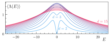
Example 1. The Lyapunov exponent takes a very simple form if is equal to the adjacency matrix of a connected -regular graph. All the vertex scattering matrices are then identical and the Gershgorin radius is for all vertices. At any given vertex, the transmission and reflection probabilities are and . The mean and local Lyapunov exponents are identical - (see Fig. 1). For the maximal Lyapunov exponent is attained at and given by the upper bound derived before in (17). Otherwise the maximal Lyapunov exponent occurs at where
| (19) |
For this is strictly smaller than the upper bound . For one has . These maximal values may be used as benchmarks for local and global Lyapunov exponents in general where one replaces by the mean degree of the graph) as any degree of non-uniformity decreases the Lyapunov exponent further. It also shows that comparing actual values of Lyapunov exponents on different graph structures needs to be performed with care. Example 2 shows how the combination of the local and global Lyapunov exponents provides a tool for analyzing the dynamics under study.
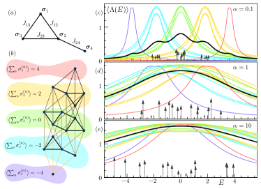
(b) Corresponding graph of the Hamiltonian where the 16 vertices correspond to spin configurations.
(c-e) Mean Lyapunov exponent (black), local Lyapunov exponents (colored lines, colours correspond to the ones used in (b)). The spectrum is located at the black arrows where the height corresponds to the participation ratio divided by . We show results for , , , and .
Example 2. Consider spins attached to vertices on a graph that interact pairwise according to the connectivity of the graph with real coupling strengths . The Hilbert space of dimension is spanned by product states with eigenvalues equal to . All spins are subject to a homogeneous magnetic field. For definiteness we choose a Hamiltonian
| (20) |
and controls the relative strength. In Fig. 2 we show the mean and local Lyapunov exponents for a particular choice of the spin graph and some values of the interaction strength . The figure shows that the mean Lyapunov exponent remains much smaller than the maximal local one for a weak coupling where eigenstates remain mainly within a subspace of constant while stronger couplings lead to more uniform distributions.
Example 3. The GE ensemble [6] of tridiagonal matrices offers a simple case for studying the the local Lyapunov exponent when the Hamiltonian consists of independently distributed random entries. The diagonal are distributed normally with zero mean and variance . The off-diagonal elements are distributed with . is a parameter which characterize the ensemble. The spectral statistics coincides with the counterpart Wigner-Dyson ensembles for .For large one finds to leading order
| (21) |
While the mean of is growing as , its variance tends to a constant. Hence, by increasing , the mean value of the off-diagonal entries become increasingly dominant, and the effect of fluctuations diminish. This leads to the mean field discrete Schrödinger equation
| (22) |
with . For the ODE analogue of (22) reads
| (23) |
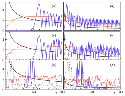
It describes a particle with “energy” subject to a potential , with classical turning point at . Fig. 3(a-b) show the absolute square values of the eigenfunctions and the Lyapunov exponents for (22) for two eigenvalues which belong to the higher (left) and lower (right) parts of the spectrum. The main feature is the appearance of domains on the axis where the eigenvector amplitudes are small. The domains starts at and extend to larger values as the spectral parameter increases. The local Lyapunov exponents follow this behavior, indicating that the phenomenon is captured by the underlying classical dynamics. This feature can be derived from a uniform semi-classical analysis [22]. The turning point occurs at where .
Fig. 3(c-f) show results for individual realizations of the ensemble for comparison. Fig 3 (c-d) are computed for . The wave functions and the local Lyapunov exponents are rather similar to their counterpart shown in Fig. 3(a-b), albeit more noisy. Fig 3 (e-f) are computed for . It displays a radically different behavior because for low values of the random potential dominates leading to localization of the wave functions. Note that the dependence on is through its square root, so the actual effect of changing is only a factor . Averaging over many realizations the Lyapunov exponents approach the results obtained for the mean potentials. Once the interaction is composed of classical and purely quantum effects, the local Lyapunov exponents give a good indication of the effects due to the former.
Summary and Discussion – We defined a classical stochastic process for a given Hermitian matrix. This gives an alternative quantum-classical correspondence to standard classical limits and exists where the latter cannot be defined. Lyapunov exponents for the classical process were derived, and studied for some examples. They are easy to compute from the given matrix and do not require involved numerical methods. We demonstrated the sensitivity of the Lyapunov exponents to localization properties of the eigenstates. The Lyapunov exponents thus form a very useful tool to analyze quantum dynamics from the perspective of quantum chaos.
Moreover, this new tool opens many new avenues for further research and we conclude this letter with a few questions that need to be addressed but will be deferred for a future publication. For example, how is this alternative quantum-classical correspondence related to OTOC? What additional information is stored in the variance of the Lyapunov exponent? And many more.
Acknowledgment
We are indebted to Omri Sarig for clarifying several issues in ergodic theory and to Sasha Sodin for discussing some of his new results on the GE model before publication, to Hans Weidenmüller who recommended corrections to an early draft of the manuscript, to Micha Barkooz for discussing the relation to the OTOC approach, and to Tomasz Maciążek and to Yiyang Jia for sharing with us their many spins models.
References
- [1] E. Ott, Chaos in Dynamical Systems (2nd ed, Cambridge University Press, 2002).
- [2] P. Cvitanović, R. Artuso, R. Mainieri, G. Tanner, G. Vattay, Chaos: Classical and Quantum, ChaosBook.org (Niels Bohr Institute, Copenhagen 2020).
- [3] M. Gutzwiller Chaos in Classical and Quantum Mechanics (Springer, 1990).
- [4] F. Haake, S. Gnutzmann, M. Kuś, Quantum Signatures of Chaos, (4th ed, Springer, 2018)
- [5] O. Bohigas, M.J. Giannoni, C. Schmit, Characterization of chaotic quantum spectra and universality of level fluctuation laws, Phys. Rev. Lett. 52, 1 (1984).
- [6] I. Dumitriu, A. Edelman, Matrix models for beta ensembles, J. Math. Phys. 43, 5830 (2002).
- [7] A.I. Shnirelman, Ergodic properties of eigenfunctions [in russian], Uspekhi Mat. Nauk. 29, 181 (1974).
- [8] Y. Breuer, P. Forrester, U. Smilansky, Random discrete Schrödinger operators from random matrix theory, J. Phys A 40, F161 (2007).
- [9] A. Larkin, Y.N. Ovchinnikov, Quasiclassical method in the theory of superconductivity, JETP 28, 960 (1969).
- [10] S.H. Shenker, D. Stanford, Black holes and the butterfly effect, JHEP 3, 067 (2014).
- [11] J. Maldacena, S.H. Shenker, D. Stanford, A bound on chaos, JHEP 8, 106 (2016).
- [12] A. Kitaev, A simple model of quantum holography, talk given at KITP Program: Entanglement in Strongly-Correlated Quantum Matter, Vol. 7 (USA April, 2015).
- [13] K. Hashimoto, K.-B. Huh, K.-Y. Kim, R. Watanabe, Exponential growth of out-of-time-order correlator without chaos: the inverted harmonic oscillator, JHEP 11, 068 (2020).
- [14] A. Bhattacharyya, W. Chemissany, S.S. Haque, J. Murugan, B. Yan, The multi-faceted inverted harmonic oscillator: Chaos and complexity, SciPost Physics Core 4, 002 (2021).
- [15] S. Gerschgorin, Über die Abgrenzung der Eigenwerte einer Matrix [in german], Izv. Akad. Nauk. USSR Otd. Fiz.-Mat. Nauk 6, 749–754 (1931).
- [16] U. Smilansky, Quantum chaos on discrete graphs, J. Phys. A 40, F621 (2007).
- [17] S. Gnutzmann, U. Smilansky, Trace formulas for general hermitian matrices, J. Phys. A 53, 035201 (2020).
- [18] F. Barra, P. Gaspard, Classcial Dynamics on Graphs, Phys. Rev. A 63, 066215 (2001).
- [19] P. Walters, An Introduction to Ergodic Theory (Springer, New York, 1982).
- [20] W. Parry, M. Pollicott, Zeta Functions and the Periodic Orbit Structure of Hyperbolic Dynamics, (Société Mathématique de France, 1990).
-
[21]
Omri Sarig, Lecture notes on Ergodic Theory,
Weizmann Institute (2023),
https://www.weizmann.ac.il/math/sarigo/lecture-notes. - [22] S. Sodin, O. Zeitouni, On the shape of the eigenvectors of tridiagonal GE matrices, to be published.
- [23] Sven Gnutzmann and Uzy Smilansky, To be published (2024).