Gridsemble: Selective Ensembling for
False Discovery Rates

Abstract

In this paper, we introduce Gridsemble, a data-driven selective ensembling algorithm for estimating local false discovery rates (fdr) in large-scale multiple hypothesis testing. Existing methods for estimating fdr often yield different conclusions, yet the unobservable nature of fdr values prevents the use of traditional model selection. There is limited guidance on choosing a method for a given dataset, making this an arbitrary decision in practice. Gridsemble circumvents this challenge by ensembling a subset of methods with weights based on their estimated performances, which are computed on synthetic datasets generated to mimic the observed data while including ground truth. We demonstrate through simulation studies and an experimental application that this method outperforms three popular R software packages with their default parameter values—common choices given the current landscape. While our applications are in the context of high throughput transcriptomics, we emphasize that Gridsemble is applicable to any use of large-scale multiple hypothesis testing, an approach that is utilized in many fields. We believe that Gridsemble will be a useful tool for computing reliable estimates of fdr and for improving replicability in the presence of multiple hypotheses by eliminating the need for an arbitrary choice of method. Gridsemble is implemented in an open-source R software package available on GitHub at jennalandy/gridsemblefdr.

Keywords False Discovery Rates  $\cdot$ Multiple Hypothesis Testing  $\cdot$ Model Selection  $\cdot$ Ensembling

1 Introduction

Multiple hypothesis testing problems are common when working with high-dimensional data across a range of scientific fields. For example, in high throughput transcriptomics, a common question is which of many genes are expressed differently between two groups, such as two cell types. This biological question can be translated to a statistical problem: for each gene, test a null hypothesis of equal mean expression between the groups against a two-sided alternative. With many hypotheses being tested at once, typically on the order of thousands, the number of falsely rejected hypotheses can grow unreasonably large, and accounting for multiplicities is recommended in order to draw reliable inferences based on significance testing (Dudoit et al., 2003; Farcomeni, 2008). More generally, controlling for multiplicities has been identified as one of the potential remedies to the so-called replicability crisis in fields including biology, sociology, psychology and others (Committee on Reproducibility and Replicability in Science, 2019).

Early approaches account for multiplicities by controlling the Type-I error rate of the set of hypotheses. Examples include setting a family-wise error rate (FWER) (Tukey, 1953, 1991) or a global false discovery rate (FDR) (Benjamini and Hochberg, 1995) to adjust p-values or significance cutoffs. Tail-end (Fdr) (Benjamini and Hochberg, 1995) and local (fdr) (Efron et al., 2001) false discovery rates are instead reported for each hypothesis and can be used in place of p-values to quantify evidence against the null. All of these quantities are unknown, as they rely on the unobservable truths of hypotheses, so they must be estimated or bounded for practical application. In this paper, we focus on local false discovery rates (fdr) estimation, which can in turn be leveraged for Fdr and FDR estimation.

An fdr model takes in a set of test statistics and returns fdr estimates as well as an estimate of the proportion of hypotheses that are null. In practice, there are many models to choose from, the most popular of which are implemented in the R software packages locfdr (Efron et al., 2015), fdrtool (Klaus and Strimmer, 2021; Strimmer, 2008), and qvalue (Storey et al., 2015). Each software package and choice of parameter values may result in very different fdr estimates and thus different conclusions as to which hypotheses are rejected. For example, in the dataset of Section 5, one model estimates that only 6% of hypotheses are null, while another estimates that 100% are null.

To choose an fdr model, we need to understand the performance of each model on the given data set. However, hypotheses and therefore fdr’s are not observable, meaning a model’s performance cannot be estimated empirically. Currently, there is limited practical guidance on which models to use and under what conditions, making this an arbitrary choice that may have substantial consequences on conclusions.

In this paper, we address this challenge through a selective ensembling approach called gridsemble with three main components: 1) generation of synthetic datasets that mimic observed data but include ground truth, 2) estimation of model performances using these datasets and selection of a high-performing subset of models, and 3) weighted ensembling of these models’ estimates. Our simulation studies and an experimental application show that this method outperforms three popular R software packages with their default parameter values, both in terms of the estimated fdr and the downstream classification of hypotheses. Furthermore, this method eliminates the need for an arbitrary choice of model, improving replicability in the presence of multiple hypotheses. An R software package for gridsemble is publicly available on GitHub at jennalandy/gridsemblefdr.

2 Definitions and Motivation

2.1 False Discovery Rates

Consider a collection of $I$ null hypotheses $H_{01},\ldots,H_{0I}$, associated test statistics $u_{1},\dots,u_{I}$, and rejection regions $R_{1},\dots,R_{I}$ produced by some testing procedure. False discovery rate methodologies encompass various estimands of interest, reviewed next.

The global false discovery rate (FDR) is the unknown overall proportion of null hypotheses among those whose test statistics fall into their rejection regions (Benjamini and Hochberg, 1995), that is:

$$\mbox{global FDR}=\frac{\sum_{i=1}^{I}\mathbf{1}\{u_{i}\in R_{i}\cap H_{0i}\}}{\sum_{i=1}^{I}\mathbf{1}\{u_{i}\in R_{i}\}},$$ (1)

where $\mathbf{1}$ is a binary indicator of its argument. Here, a single value refers to the group of hypotheses.

Tail-end (Fdr) (Efron and Tibshirani, 2002) and local (fdr) (Efron et al., 2001) false discovery rates are reported for each hypothesis. The tail-end Fdr for hypothesis $i$ is the unknown proportion of hypotheses that are null among those with test statistics as or more extreme than $u_{i}$, assuming that all statistics are on a comparable scale (Benjamini and Hochberg, 1995). When large magnitudes of $u$’s denote more extreme departures from the null, we have:

$$\mbox{Tail-end Fdr}(u_{i})=\frac{\sum_{i^{\prime}=1}^{I}\mathbf{1}\{|u_{i^{\prime}}|\geq|u_{i}|\cap H_{0i^{\prime}}\}}{\sum_{i^{\prime}=1}^{I}\mathbf{1}\{|u_{i^{\prime}}|\geq|u_{i}|\}}.$$ (2)

Quantities (1) and (2) are defined as $0$ when their denominator is $0$.

Local fdr is approximately the proportion of null hypotheses in the vicinity of $u_{i}$. A commonly made assumption is that the test statistics come from a continuous mixture distribution with components $f_{0}(u)$ and $f_{1}(u)$, describing the distributions of test statistics generated by null and alternative hypotheses, respectively. The mixing parameter $\pi_{0}$ is the unknown proportion of null hypotheses. Then, local false discovery rates can be defined with Bayes rule as:

$$\mbox{fdr}(u_{i}) =\pi_{0}f_{0}(u_{i})/f(u_{i}),$$ (3)

where

$$f(u_{i})=\pi_{0}f_{0}(u_{i})+(1-\pi_{0})f_{1}(u_{i}).$$ (4)

In most implementations, fdr’s are estimated from test statistics $\mathbf{u}$ alone (Efron et al., 2015; Klaus and Strimmer, 2021; Storey et al., 2015), though important variations exist (Stephens, 2016-10).

2.2 Estimating fdr

Estimating local fdr takes advantage of the large number of hypotheses with an empirical Bayes approach (Efron et al., 2001), first estimating $f$ and $\pi_{0}f_{0}$ using all $\mathbf{u}$, then evaluating Equation 3 at each $u_{i}$ to obtain a vector of estimates, $\widehat{\mathbf{fdr}}$. Different R software packages, and within them parameter values, use different estimation methods, distributional assumptions, and subsets of the data in estimating $f$ and $\pi_{0}f_{0}$. Importantly, different models can return very different estimates, and thus can lead to different conclusions.

Estimates of fdr can be leveraged to additionally estimate Fdr and FDR. Again assuming large magnitudes of $u$ denote more extreme departures from the null, we have the relation

$$\mbox{Fdr}(u_{i})=E_{f}\left[\hbox{fdr}(U)\Big{|}|U|\geq|u_{i}|\right],\;\;\;\;\;\text{where }U\sim f.$$ (5)

Thus, estimates of fdr can easily be converted into estimates of Fdr via:

$$\widehat{\mbox{Fdr}}(u_{i}) =\frac{\sum_{i^{\prime}=1}^{I}\mathbf{1}\{|u_{i^{\prime}}|\geq|u_{i}|\}\widehat{\hbox{fdr}}_{i^{\prime}}}{\sum_{i^{\prime}=1}^{I}\mathbf{1}\{|u_{i^{\prime}}|\geq|u_{i}|\}}$$ (6)

Additionally, if the rejection region is $R_{i}=\{|u_{i}|\geq|u_{0}|\}$ for all tests, then $\widehat{\mbox{Fdr}}(u_{0})$ estimates global FDR. These quantities can also be estimated using Bayesian decision theoretic approaches (Müller et al., 2007).

2.3 Model Subset Selection and Ensembling

An fdr model is indexed by $\theta$, a combination of software package and parameter values. Evaluating model $\theta$ given the observed test statistics $\mathbf{u}$ returns estimates of local fdr values as well as an estimate of $\pi_{0}$, denoted by $\widehat{\mathbf{fdr}}_{\theta}(\mathbf{u})$ and $\widehat{\pi}_{0\theta}(\mathbf{u})$, respectively.

If true $\mathbf{fdr}$ is known, we can evaluate the performance of a model by a loss function ${L:\mathbb{R}^{N}\times\mathbb{R}^{N}\rightarrow\mathbb{R}}$ mapping model predictions $\widehat{\mathbf{fdr}}$ and true $\mathbf{fdr}$ to a real number representing prediction error or the information lost. The objective we aim to minimize is the expected loss, $\mathcal{L}=E_{\mathcal{P}}[L(\widehat{\mathbf{fdr}},\mathbf{fdr})]$. Here, $\mathcal{P}$ is the true data generating function for $\{\mathbf{u},\mathbf{fdr},\mathbf{l}\}$, where $l_{i}=1-\mathbf{1}\{H_{0i}\}$.

A common approach in model selection is a grid search, which exhaustively considers all combinations of parameters and orders models from best to worst by estimated objective (Yu and Zhu, 2020). When true outputs can be observed, the objective can be estimated empirically by the loss in a held-out portion of the data (Kuhn et al., 2013). In some cases, the objective is estimated by the loss in external datasets (Nomura and Saito, 2021) or synthetic datasets constructed by bootstrap or jackknife resampling (Efron, 1982; Kohavi et al., 1995). However, true $\mathbf{fdr}$ is unknown, making this challenging.

An alternative to selecting a single model is to combine, or ensemble, estimates from multiple models. The literature on ensembling is extensive (Dong et al., 2020) and shows that ensembling over all possible models with weights corresponding to model performance can improve predictive ability over using a single model. Further improvement can be seen when being selective to only include well-performing models in an ensemble, as, for example, in Occam’s window (Madigan and Raftery, 1994).

2.4 Motivation

The motivation for this work is the need for a practical and data-driven approach to estimate fdr in the current landscape. Models disagree, and their relative merits vary widely across data applications. Because fdr is not observed, model performances cannot be assessed empirically. Instead, we estimate model performances using synthetic datasets generated to mimic the observed data while including ground truth, and we ensemble a high performing subset of models to arrive at more robust and replicable estimates.

3 Gridsemble

Gridsemble is a selective ensembling algorithm for estimating fdr in large-scale multiple hypothesis testing. First, we generate synthetic datasets with both test statistics $\mathbf{u}$ and ground truth $\mathbf{fdr}$ through a parametric bootstrap, where the parametric working model is fit on observed test statistics. Next, we estimate model performances using these datasets and select a high performing subset of models. Finally, we ensemble the estimates from selected models with a weighted average where weights are proportional to model performances.

Our work focuses on two-sided hypotheses where the distribution of test statistics is centered at zero under the null and large magnitudes provide evidence against the null. In the context of differential expression, this includes two-sample t-tests (Ryu et al., 2002; Cui and Churchill, 2003) and log fold change estimates from over-dispersed log-linear models (Lu et al., 2005; Robinson and Smyth, 2007) such as from R software packages EdgeR (Chen et al., 2020) and DESeq2 (Varet et al., 2016).

We consider fdr models implemented by two R packages that estimate fdr from this type of test statistic: locfdr (Efron et al., 2015) and fdrtool (Klaus and Strimmer, 2021; Strimmer, 2008). A third R package, qvalue (Storey et al., 2015), instead takes in p-values, but we still recognize it as a widely used and valuable implementation. We incorporate qvalue by converting statistics $\mathbf{u}$ to p-values. In the gridsemble R package, the user may provide their own function to convert statistics to p-values, but the results presented assume a t-distributed null (or a standard Normal if degrees of freedom are not provided). We acknowledge that these p-values are only valid when statistics are t-distributed, and conjecture that the poorer results of qvalue in some of our simulation studies may be attributable to this conversion rather than to qvalue itself. We highlight, though, that gridsemble is able to rule out fdr models from qvalue when such conversion is not appropriate.

We use a grid of $M=292$ models, which includes the three packages with all possible combinations of categorical parameters and equally spaced choices of numeric parameters. For a given dataset, we exclude models that do not converge or produce errors. There are three key steps to this approach, summarized next: fitting the working model, selecting a subset of models, and ensembling. Algorithm 1 outlines the method.

Step 1: A working model is defined as a mixture of two components. The first, $f_{W0}(u|\phi_{0})$, corresponding to statistics under the null hypothesis, is Normal and centered at zero. The second, $f_{W1}(u|\phi_{1})$, corresponding to statistics under the alternative hypothesis, is a Non-Local Normal (Rossell and Telesca, 2017), which is symmetric with density away from zero. The mixture model is completed by the mixture weight $\pi_{0}$, defined earlier. For conciseness, $\phi=(\phi_{0},\phi_{1},\pi_{0})$, and $f_{W}(u|\phi)$ is the implied marginal. This model is fit to the observed statistics with the Expectation-Maximization (EM) algorithm (Dempster et al., 1977). Conditional on the working model, we can generate synthetic datasets comprising statistics $\mathbf{u}$, as well as $\mathbf{fdr}$ and hypothesis labels $\mathbf{l}$. $N$ synthetic datasets are generated from the working model. This working model is separate from the fdr estimation models.

Step 2: We select a subset of models with the smallest estimated objectives. For each fdr model, the estimated objective is the model loss (in our applications, MSE) averaged across the synthetic datasets. This estimate is unbiased if the working model is the same as the true data generating model (Section 7.5.1). A subset of the $m$ highest performing models is selected. Based on simulation studies, we use $N=10$ synthetic datasets and $m=10$ selected models.

Step 3: The best $m$ models are combined in an ensemble. Model weights are inversely proportional to their estimated objectives. The ensemble helps to account for uncertainty in the estimated objectives, in contrast to relying only on the single model with minimum estimated objective.

The gridsemble approach could be extended to other types of test statistics with adjustments to the working model and the grid of possible fdr models. The null and alternative components of the working model should match the assumed low- and high-evidence regions of the test statistic. Each model in the grid must be able to use the test statistic as input, possibly after a conversion, as seen with qvalue here.

Algorithm 1 – Gridsemble
Input: Observed test statistics $\mathbf{u}$, number of synthetic datasets $N$, loss function $L$, ensemble size $m$, grid of model specifications $\Theta$ where $||\Theta||=M\geq m$
Output: $\widehat{\textbf{fdr}}$, $\widehat{\textbf{Fdr}}$ and $\widehat{\pi}_{0}$

1: # Step 1: Working Model

2:$\hat{\phi}\leftarrow$ MLE of $\phi$ under the working model with data $\mathbf{u}$ via Expectation-Maximization (EM) algorithm

3:for $n=1,\dots,N$ do

4:     Draw synthetic data $\{\mathbf{u}^{n},\mathbf{fdr}^{n},\mathbf{l}^{n}\}$ given $\hat{\phi}$

5:

6:# Step 2: Model Subset Selection

7:for $\theta\in\Theta$ do

8:     $\widehat{\mathcal{L}}(\theta)\leftarrow\frac{1}{N}\sum_{n=1}^{N}L(\widehat{\mathbf{fdr}}_{\theta}(\mathbf{u}^{n}),\mathbf{fdr}^{n})$

9:Sort models such that $\widehat{\mathcal{L}}(\theta_{(1)})\leq\widehat{\mathcal{L}}(\theta_{(2)})\leq\dots\leq\widehat{\mathcal{L}}(\theta_{(M)})$ and select $\Theta^{*}=\{\theta_{(1)},\dots,\theta_{(m)}\}$

10:

11:# Step 3: Ensemble

12:Compute model weights $w_{\theta}=\frac{1/\widehat{\mathcal{L}}(\theta)}{\sum_{\theta\in\Theta^{*}}1/\widehat{\mathcal{L}}(\theta)}$    $\forall\theta\in\Theta^{*}$

13:$\widehat{\mathbf{fdr}}=\sum_{\theta\in\Theta^{*}}w_{\theta}\;\widehat{\mathbf{fdr}}_{\theta}(\mathbf{u})$

14:$\widehat{\hbox{Fdr}}_{i}=\frac{\sum_{i^{\prime}=1}^{I}\mathbf{1}\{|u_{i^{\prime}}|\geq|u_{i}|\}\widehat{\hbox{fdr}}_{i^{\prime}}}{\sum_{i^{\prime}=1}^{I}\mathbf{1}\{|u_{i^{\prime}}|\geq|u_{i}|\}}$

15:$\widehat{\pi}_{0}=\sum_{\theta\in\Theta^{*}}w_{\theta}\widehat{\pi}_{0,\theta}(\mathbf{u})$

16:Return $\widehat{\text{{fdr}}}$, $\widehat{\textbf{Fdr}}$, and $\widehat{\pi}_{0}$

4 Simulation Studies

4.1 Simulated Data

We consider three simulation studies to evaluate the performance of gridsemble on different types of data. For each, we simulate $200$ repetitions of $I=1000$ hypotheses.

Symmetric: In the symmetric simulation study, 80% of hypotheses are null ($\pi_{0}=0.8$). Based on Strimmer (2008), statistics from null hypotheses follow a Normal distribution with mean zero and those from alternative hypotheses follow a mixture of Uniforms away from zero. Specifically:

$$f_{0}=N(\mu=0,\sigma=3)$$

$$f_{1}=\frac{1}{2}U(-12,-4)+\frac{1}{2}U(4,12).$$

Asymmetric: In the asymmetric study, $\pi_{0}=0.85$. The majority of alternative hypotheses have positive test statistics, but the range of negative statistics is wider. Specifically:

$$f_{0}=N(\mu=0,\sigma=2)$$

$$f_{1}=\frac{1}{3}U(-12,-5)+\frac{2}{3}U(3,9).$$

Curated Ovarian Data (COD) Based: The COD-based simulation study comes from real gene expression data with induced differential expression. We start with the TCGA expression set of 13,104 genes across 578 samples provided by the curatedOvarianData R software package (Ganzfried et al., 2013). We randomly assign group labels with approximately equal group sizes, and twenty percent of genes are sampled to be differentially expressed ($\pi_{0}=0.8$). Differential expression is induced in each gene by multiplying expression levels in one group by a scalar, sampled to be unique for each gene. A two-sample t-test is then computed for each gene. Group labels, sampled genes, and scalars are different for each repetition.

4.2 Benchmarks and Partial Implementations

As benchmarks, we use the three R packages, locfdr, fdrtool, and qvalue, with their default parameter values. Without existing guidance on model selection for fdr, these benchmarks reflect common choices in practice.

To investigate gridsemble’s performance gain due to ensembling versus model selection, we investigate three partial implementations. grid is the single model with the best estimated objective, only utilizing model selection. ensemble is an equally-weighted ensemble over ten randomly chosen models, only utilizing ensembling and using the same ensemble size as gridsemble. ensemble_all is an equally weighted ensemble over all models in the grid (up to 292).

4.3 Evaluation

We evaluate fdr estimation approaches using five metrics. fdr RMSE is the root mean squared error between the estimated and true local fdr values. The true fdr can be calculated only for symmetric and asymmetric studies using the known distributions of test statistics. For the COD-based study, we instead look at Fdr RMSE as the RMSE between estimated and empirical tail-end Fdr values. These metrics are important for the goal of accurate Fdr and fdr estimates. The next three metrics are important for the goal of accurate classifications of hypotheses into null versus alternative. PR AUC and ROC AUC are the areas under the precision-recall and receiver operating characteristic curves, respectively. Test label Brier score is the average squared distance between the positive predictive values, $1-\widehat{\mathbf{fdr}}$, and binary test labels, $\mathbf{l}$.

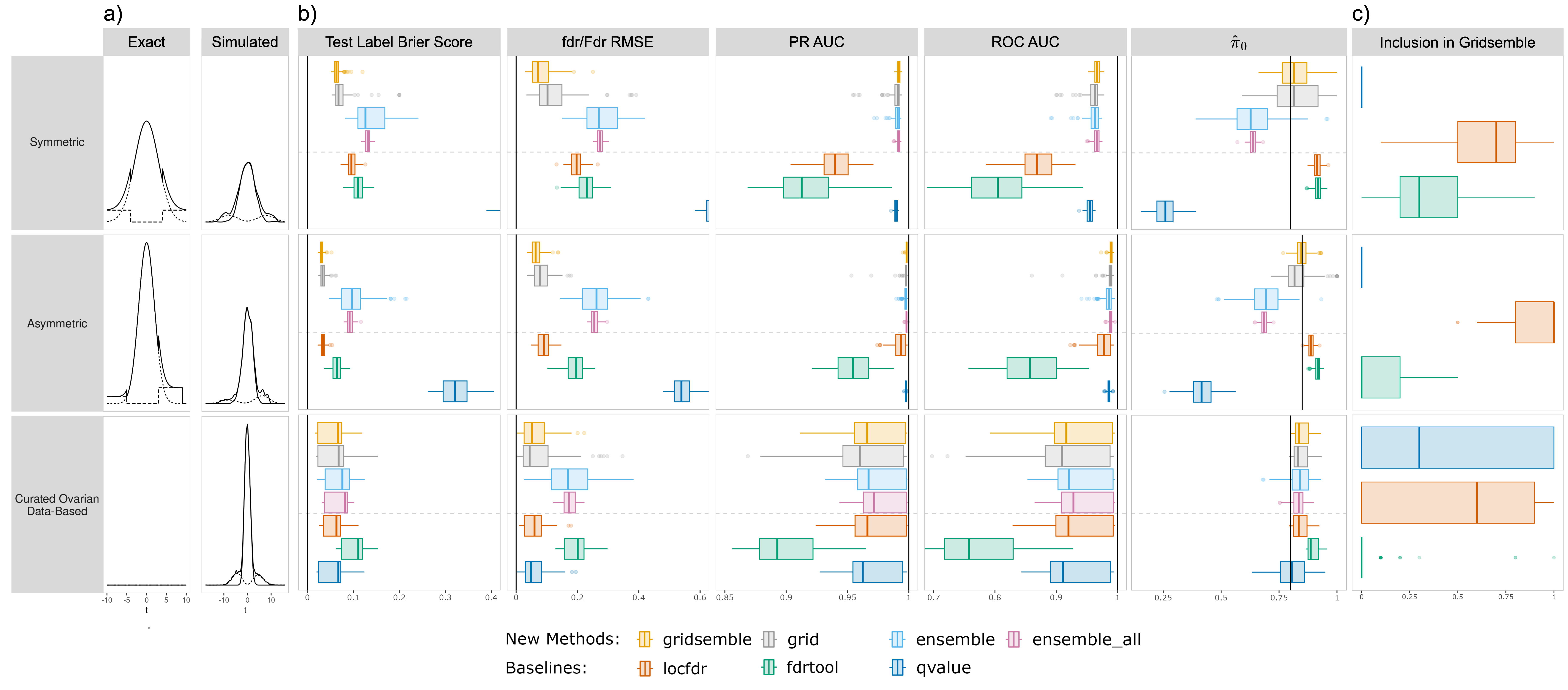
Figure 1: a) Simulation study distributions. Exact densities (left) and a single simulated example (right) for symmetric, asymmetric and curated ovarian data-based simulation studies. Plotted are mixtures (solid) and weighted nulls (dotted) and alternatives (dashed). b) Simulation study results of gridsemble and partial implementations grid, ensemble, and ensemble_all (above dashed line) versus each of the benchmarks locfdr, fdrtool, and qvalue (below dashed line) with their default parameters. Plotted are metrics of interest (test label Brier score, fdr or Fdr RMSE, and areas under the PR and ROC curves) and estimated $\pi_{0}$ over 200 repetitions. Optimal values of are indicated with black vertical lines. For exact values of medians, see Supplementary Table 1. c) Proportion of models from each package included in gridsemble over 200 repetitions. Key results include the improvement of median gridsemble over benchmark methods in most cases, indicating gridsemble performs better than existing packages with their default parameters, as well as frequent improvement of gridsemble over partial implementations, indicating the need for our joint approach utilizing both model subset selection and an ensemble. gridsemble also estimates $\pi_{0}$ as or more accurately than other methods.

4.4 Results

Figure 1 summarizes simulation study results. Comparing median metrics, gridsemble outperforms benchmarks in all simulation studies for most metrics (Figure 1b). The variation around the median shows that gridsemble may be outperformed by one of the benchmarks, but the magnitudes of potential losses are much smaller than the magnitudes of potential improvements. gridsemble outperforms baselines by as much as 0.62 points in median fdr RMSE (compared to qvalue in the symmetric study), as much as 0.09 in median PR AUC (compared to fdrtool in the COD-based study), as much as 0.20 in median ROC AUC (compared to fdrtool in the COD-based study), and as much as 0.39 in median test label Brier score (compared to qvalue in the symmetric study). In the other direction, the worst case is that gridsemble perfoms only up to 0.001 points worse in median fdr RMSE (compared to qvalue in the COD-based study), 0.005 points worse in median PR AUC (compared to locfdr in the COD-based study), and 0.007 points worse in median ROC AUC (compared to locfdr in the COD-based study). gridsemble is never worse than the benchmarks in terms of median test label Brier score. In terms of estimated $\pi_{0}$, gridsemble performs similarly to or better than other methods, and is only slightly outperformed by qvalue in the COD-based study.

gridsemble also outperforms each partial implementation (Figure 1b). The improvement of gridsemble over grid and ensemble emphasizes the utility of combining the model subset selection and ensemble procedures . The improvement of gridsemble over ensemble_all highlights that being selective over which models to included in an ensemble is more important than increasing ensemble size.

Finally, we see that gridsemble is able to selectively avoid packages whose models perform poorly on the data at hand (Figure 1c). qvalue performs poorly on the symmetric and asymmetric studies due to our improper conversion of test statistics to p-values, and models from qvalue do not appear in the subset of models selected by gridsemble. Similarly, fdrtool doesn’t perform well in the COD-based study, and its models are almost always excluded from gridsemble’s selection. This gives insight into how gridsemble functions to preferentially include models that work well on a given dataset and exclude models that don’t.

5 Experimental Application

5.1 Data

The Platinum Spike dataset (Zhu et al., 2010) is an experimental spike-in study of 18 Affymetrix Drosophilia Genome 2.0 microarrays under two conditions. There are three observations for each condition with three technical replicates per observation. 36.2% of these genes are differentially expressed with fold changes between 0.25 and 3.5. Expression data are available on GEO Browser as GSE21344 and the fold change data is in an additional file of the Platinum Spike paper (Zhu et al., 2010).

We aggregate the 535,824 Affymetrix probes over 18,952 genes using robust multi-array average expression measure (Irizarry et al., 2003). We remove empty probe sets, those assigned to multiple clones, and those whose clones have multiple fold change values. This results in expression measures for 5,370 genes across our 18 samples. We then average across technical replicates and compute a two-sample t-statistic for each gene.

5.2 Analysis

The Platinum Spike dataset allows us to look at real differential gene expression data and to perform multiple hypothesis testing with known labels of which hypotheses are null and alternative. However, this dataset has a proportion of null hypotheses $\pi_{0}=0.64$, while “practical applications of large-scale testing usually assume a large [$\pi_{0}$ above] 0.9” (Efron, 2007). To evaluate gridsemble and benchmark methods on real differential expression data with a practical $\pi_{0}$, we sample subsets of genes to construct datasets with varying $\pi_{0}$.

We consider true $\pi_{0}$’s between 0.6 and 0.95. For each $\pi_{0}$, we sample ten subsets of 1000 genes. On each, we evaluate methods with Fdr MSE, test label Brier score, PR AUC, and ROC AUC. We also report calibration results, summarized with the slope and intercept of a logistic regression model predicting hypothesis labels from estimated log odds, $\mbox{ln}((1-\widehat{\mathbf{fdr}})/\widehat{\mathbf{fdr}})$ (Steyerberg and Vergouwe, 2014). Perfectly calibrated $\widehat{\mathbf{fdr}}$ would have an intercept of 0 and a slope of 1.

Finally, we examine the downstream utility of $\widehat{\mathbf{fdr}}$ in classifying hypotheses as null or alternative. We consider three cutoffs for classification: first, the standard cutoff of 0.2 recommended in (Efron, 2007), second, a cutoff chosen so that $\widehat{\pi}_{0}$ proportion of tests are classified as null, and third, an oracle cutoff chosen so that true $\pi_{0}$ proportion of genes are classified as null. In summary, cutoffs are:

$$c^{(standard)} =0.2$$ (7)

$$c^{(\widehat{\pi}_{0})}(\widehat{\mathbf{fdr}}) =(1-\widehat{\pi}_{0})*100\text{th quantile of }\widehat{\mathbf{fdr}}$$

$$c^{(\pi_{0})}(\widehat{\mathbf{fdr}}) =(1-\pi_{0})*100\text{th quantile of }\widehat{\mathbf{fdr}}$$

and classification rules, for a given cutoff $c$, are:

$$\hat{l}_{i}=\begin{cases}\hbox{null}&\hbox{ if }\widehat{\hbox{fdr}}_{i}>c\\ \hbox{not null}&\hbox{ if }\widehat{\hbox{fdr}}_{i}\leq c.\end{cases}$$ (8)

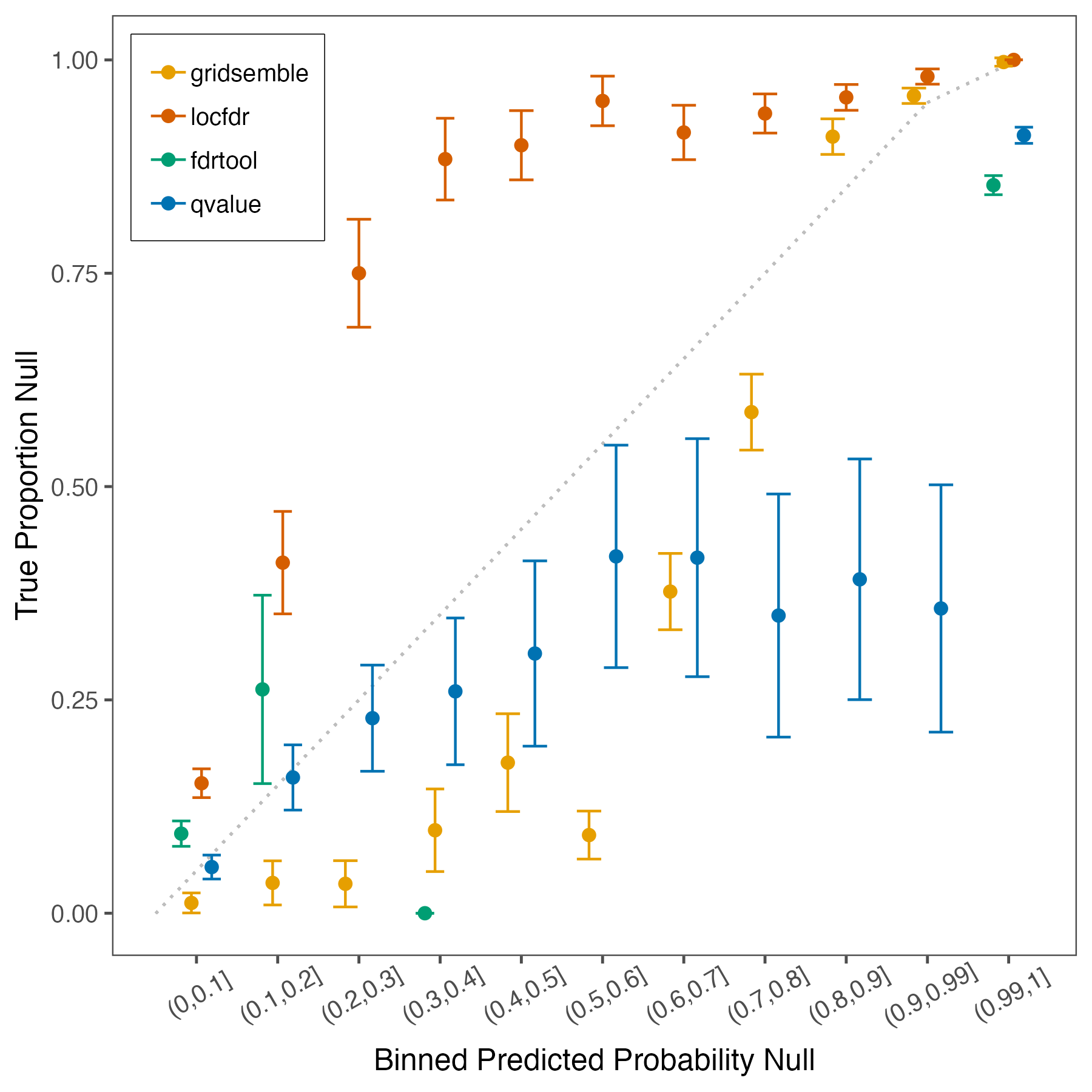
Figure 2: Calibration of experimental application results comparing gridsemble to each of the baseline methods. Plotted is the true proportion of tests which are null and a 95% binomial confidence interval for each method and bin of predicted probabilities. Perfect calibration is indicated by the dotted line. Bins are evenly spaced, with the exception of the final bin (0.99, 1], which is to emphasize how many tests have estimated fdr very close to $1$.

Results on the full Platinum Spike dataset are available in Supplementary Figure 2 and Supplementary Table 2.

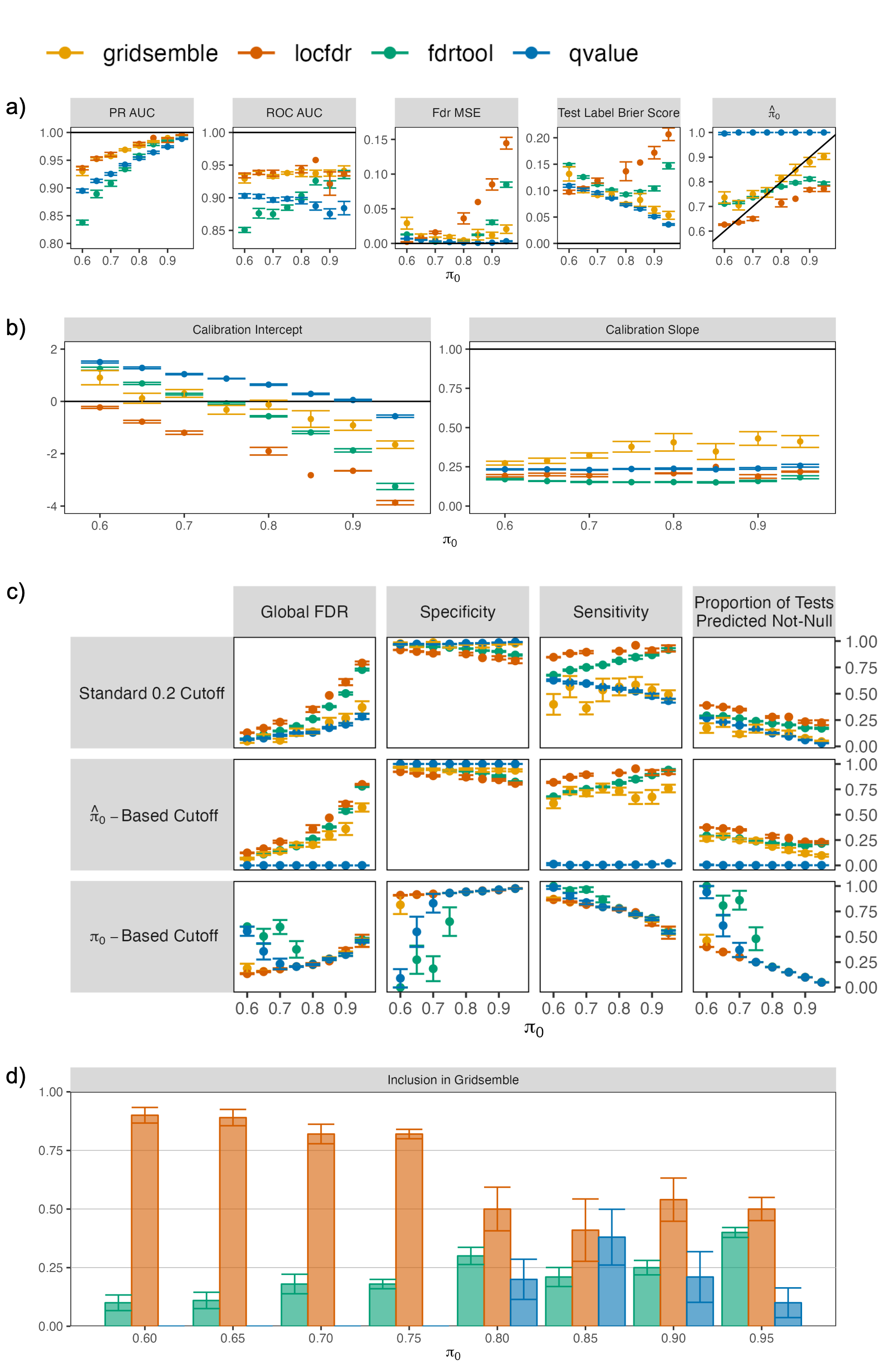
Figure 2: Results on Platinum Spike dataset. For each $\pi_{0}$, 10 subsets of the Platinum spike dataset were generated for analysis. Mean and standard error of each quantity is plotted for every $\pi_{0}$. a) Metrics on $\widehat{\mathbf{fdr}}$. b) Calibration results as summarized by the slope and intercept of a logistic regression on hypothesis labels versus estimated log odds. c) Classification metrics with three cutoff strategies: the standard 0.2 cutoff recommended in (Efron, 2007), a cutoff chosen so that the estimated $\widehat{\pi}_{0}$ proportion of tests are classified as null, and an oracle cutoff chosen so that the true $\pi_{0}$ proportion of tests are classified as null (Equation 7). We note that when $\pi_{0}$ is low and the $\pi_{0}$-based cutoff is used, the poor results of fdrtool and qvalue are due to a large proportion of their $\widehat{\mathbf{fdr}}$’s at exactly 1. The cutoff is then also 1, and all hypotheses are classified as not-null. d) Proportion of models from each package included in gridsemble for each value of $\pi_{0}$. The key result is that gridsemble performs well across all values of true $\pi_{0}$.

5.3 Results

For metrics on $\widehat{\mathbf{fdr}}$, gridsemble performs very well across values of $\pi_{0}$ (Figure 2a). Importantly, for Fdr MSE and ROC AUC, we see that gridsemble is consistent in its high performance even when other methods’ performances vary with $\pi_{0}$. Further, gridsemble yields the most consistently accurate $\pi_{0}$ estimates. These results reinforce the simulation study conclusions that gridsemble results in more accurate estimates of fdr, Fdr, and $\pi_{0}$.

The calibration results show that all methods are poorly calibrated with slopes far below 1, but gridsemble is the best (Figure 2b). The calibration intercepts are comparably good for gridsemble and qvalue, but the calibration slope is much better for gridsemble. We note that all slopes are below one, indicating that predictions are too extreme. Further, the majority of intercepts are below zero, indicating a systematic underestimation of positive predictive values, or equivalently, a systematic overestimation, or conservative estimation, of fdr.

Classification results using a cutoff based on the true $\pi_{0}$ show that for all methods and most values of $\pi_{0}$, $\widehat{\mathbf{fdr}}$ can lead to good classification metrics given the right cutoff value (Figure 2c). However, in practice, we don’t have access to the true $\pi_{0}$ values. The classification results using cutoffs based on the estimated $\widehat{\pi}_{0}$ show that in practice, gridsemble is best equipped to make an accurate cutoff decision because of its accurate $\widehat{\pi}_{0}$ estimates. gridsemble has the best global FDR and specificity without predicting all hypotheses as null like qvalue. With a cutoff of 0.2, gridsemble and qvalue perform comparably well.

The models chosen to be included in gridsemble tend to come from the packages with high performing default parameters. Figure 2d shows that models from locfdr dominate the gridsemble for low values of $\pi_{0}$, while fdrtool and qvalue are more often included for high values of $\pi_{0}$. This reinforces that gridsemble is able to preferentially select models that work best on the empirical data.

6 Discussion

We designed and evaluated gridsemble, a practical and data-driven approach to estimate local, tail-end, and global false discovery rates. These are valuable uncertainty quantifications whose practical impact is hampered by the need for an arbitrary choice of model. gridsemble overcomes this problem using a three-step approach: generating synthetic datasets, estimating model performances using these datasets and model subset selection via grid search, and an ensemble. Along with demonstrated improvement over benchmark models, this framework reduces the subjectivity of model choice, improving reproducibility. This work is implemented in an open-source R software package on GitHub at jennalandy/gridsemblefdr.

Our simulation studies and experimental application show that gridsemble generally outperforms benchmarks, but this improvement is not a guarantee. Overall, however, we observe that across simulated and experimental data, the magnitude of potential improvements is greater than the magnitude of potential losses. Two interesting results are (1) the demonstrated importance of selective model inclusion over large ensemble size and (2) the demonstrated need for our combined approach utilizing both model subset selection and ensembling.

gridsemble can serve as the blueprint for approaches using a similar architecture in at least three important dimensions: the specification of the working model, the design of the selective ensembling methodology, and the quantification of generalizability. These are briefly discussed next.

First, other distributions or fitting methods could be used for the working model. For instance, our Normal null distribution could be replaced with a t-distribution with a scale parameter to allow for heavier tails. Another option we explored is to borrow estimates from an existing fdr model. We found, though, that a working model fit from scratch does as good or better than borrowing estimates from benchmark models, especially when benchmarks severely over-estimate $\pi_{0}$. Fitting from scratch also ensures synthetic datasets are not biased towards the model the estimates came from.

Second, we chose to use a grid search for model subset selection, but could have alternatively performed a random search or Bayesian optimization (Yu and Zhu, 2020) using our estimator for the objective. Supplementary Figure 1 shows paired differences in metrics between a grid search approach and a random search approach for gridsemble and all partial implementations. We see that there is little to no change in the results of gridsemble. Bayesian optimization is challenging with categorical variables (Garrido-Merchán and Hernández-Lobato, 2020), of which we have many, so we chose not to explore this route.

Third, although this work borrows some strategies from model selection, at this time we do not perform train-test-split or cross validation. This is because we would run into the same issue that prompted the development of gridsemble itself: fdr’s are unobservable, so model performances cannot be estimated empirically on a test set. Further, we note that this would require substantial re-working of the R software packages locfdr, fdrtool, and qvalue to allow fdr estimations on new data, which is not currently supported.

Finally, along with its high performance, we emphasize that without gridsemble, practitioners must currently make arbitrary choices of what inference to report, compromising the replicability of results reported in the presence of multiplicities. A key potential impact of this work is on replicable research, through the use of a data-driven selective ensemble over a subjective human choice of model.

7 Methods

7.1 Step 1: Working Model

The working model $f_{W}$ is fit on observed test statistics and is able to generate both test statistics and associated local false discovery rates using parametric bootstrap. This “working model” (and associated parameters $\phi$) is separate from the fdr estimation “models” (indexed by $\theta$).

We use the mixture model assumption of Equation 4 with parametric specification of the components

$$f_{W}(u|\phi)=\pi_{0}f_{W,0}(u|\phi)+(1-\pi_{0})f_{W,1}(u|\phi),$$ (9)

where statistics arising from null hypotheses follow a Normal distribution centered at zero $f_{W,0}(u)=N(u;0,\sigma_{0})$ and statistics arising from alternative hypotheses follow a Non-Local Normal distribution with mass away from zero $f_{W,1}(u)=u^{2}N(u;0,\sigma_{1})/\sigma_{1}^{2}$. Mixing parameter $\pi_{0}$ is the proportion of null hypotheses.

The parameters $\phi=(\sigma^{2}_{0},\sigma^{2}_{1},\pi_{0})$ are estimated as $\hat{\phi}$ using the Expectation-Maximization (EM) algorithm (Dempster et al., 1977) on observed test statistics. Synthetic datasets $\{\mathbf{u}^{n},\mathbf{fdr}^{n},\mathbf{l}^{n}\}$ are generated from $f_{W}(u|\hat{\phi})$. First, hypothesis labels $l_{i}=1-\mathbf{1}\{H_{0i}\}$ are sampled using the estimated proportion null, $\widehat{\pi}_{0}$. Test statistics are then generated from their label-specific distributions $f_{W,0}$ or $f_{W,1}$. Local false discovery rates are then computed using Equation 3. Each synthetic dataset has the same number of hypotheses as the observed dataset, $i=1,...,I$. In summary, we draw synthetic datasets $\{\mathbf{u}^{n},\mathbf{fdr}^{n},\mathbf{l}^{n}\}$ for $n=1,\ldots N$ and $i=1,...,I$:

$$l_{i}^{n} \sim\mbox{Bernoulli}(1-\widehat{\pi}_{0})$$ (10)

$$u_{i}^{n} \sim\begin{cases}f_{W,0}(u|\hat{\phi})&\text{ if }l_{i}^{n}=0\\ f_{W,1}(u|\hat{\phi})&\text{ if }l_{i}^{n}=1\end{cases}$$

$$\mbox{fdr}_{i}^{n} =\mbox{fdr}(u_{i}^{n})=\frac{\widehat{\pi}_{0}f_{W,0}(u_{i}^{n}|\hat{\phi})}{f_{W}(u_{i}^{n}|\hat{\phi})}.$$

7.2 Step 2: Model Subset Selection

The loss of interest is mean squared error (MSE) between estimated and true fdr’s:

$$L(\widehat{\mathbf{fdr}},\mathbf{fdr})=\frac{1}{I}||\widehat{\mathbf{fdr}}-\mathbf{fdr}||^{2}_{2}$$ (11)

Our estimated objective for a given model $\theta$ is an average of empirical losses across the synthetic datasets:

$$\widehat{\mathcal{L}}(\theta)=\frac{1}{N}\sum_{n=1}^{N}\widehat{\mathcal{L}}^{n}(\theta)=\frac{1}{N}\sum_{n=1}^{N}L(\widehat{\mathbf{fdr}}_{\theta}(\mathbf{u}^{n}),\mathbf{fdr}^{n}).$$ (12)

With estimated objectives, we can reorder models such that $\hat{\mathcal{L}}(\theta_{(1)})\leq\dots\leq\hat{\mathcal{L}}(\theta_{(M)})$. We choose a subset of $m$ models with the best estimated objectives $\Theta^{*}=\{\theta_{(1)},\dots,\theta_{(m)}\}$.

7.3 Step 3: Ensemble

The $m$ models with the best estimated performances, $\Theta^{*}$, are ensembled with weights inversely proportional to their estimated objectives:

$$w_{\theta} =\frac{1/\widehat{\mathcal{L}}(\theta)}{\sum_{\theta\in\Theta^{*}}1/\widehat{\mathcal{L}}(\theta)}$$ (13)

$$\widehat{\mathbf{fdr}}(\mathbf{u}) =\sum_{\theta\in\Theta^{*}}w_{\theta}\widehat{\mathbf{fdr}}_{\theta}(\mathbf{u})$$

$$\widehat{\pi}_{0}(\mathbf{u}) =\sum_{\theta\in\Theta^{*}}w_{\theta}\widehat{\pi}_{0,\theta}(\mathbf{u})$$

We additionally estimate $\widehat{\mathbf{Fdr}}$ using Equation 6.

7.4 Implementation

The gridsemble method is implemented and publicly available in the R package gridsemblefdr on GitHub at jennalandy/gridsemblefdr. The main function takes in a vector of test statistics and returns estimates of $\pi_{0}$ and both local and tail-end false discovery rates.

7.4.1 Grid of fdr Models

Local fdr models are indexed by $\theta$, the package and parameter values. A grid of 292 models is used, including all possible combinations of categorical parameters and evenly spaced values of numeric parameters. Because fdrtool only has two parameters while locfdr and qvalue each have four, there are fewer models using the fdrtool package. In application, models that result in convergence errors on observed data are excluded.

The locfdr package (Efron, 2007) assumes a Normal distribution for the weighted null density $\pi_{0}f_{0}$. We consider four key parameters. nulltype determines whether the weighted null is estimated by maximum likelihood or central matching. pct0 determines the quantile range [pct0, 1-pct0] of central test statistics used to fit the weighted null. The default value is 0.25, and in our grid, we consider pct0 $\in$ [0, 0.3]. type determines whether the marginal density $f$ is fit with a natural spline or polynomial model. pct is the proportion of outliers excluded when fitting the marginal density. The default value is 0, and in our grid, we consider pct $\in$ [0, 0.3]. Out of the full grid of 292 models, 150 use locfdr.

The fdrtool package (Strimmer, 2008; Klaus and Strimmer, 2021) also assumes a Normal distribution for the weighted null, but uses a non-parametric Grenander estimator for the marginal density. We consider two key parameters. cutoff.method chooses the method that determines which central test statistics to use when fitting the weighted null. If the cutoff.method = "pct0", then pct0 defines the proportion of central statistics used to fit the null. We consider pct0 $\in$ [0.4, 1], matching the range used in locfdr. Out of the full grid of 292 models, 22 use fdrtool.

The qvalue package (Storey et al., 2015) takes in p-values and estimates the weighted null p-value density as a Uniform distribution. It uses a natural spline to fit the marginal density. We consider four key parameters. pi0.method determines whether to use a bootstrap or a smoother to tune a parameter used to estimate $\pi_{0}$. transf is whether a probit or logit transformation is applied to the p-values. adj defines the smoothing bandwidth used in the full density estimation. The default value is 1.5, and we consider values of adj $\in$ [0.5, 2]. If pi0.method = "smoother", then smooth.log.pi0 controls whether a smoother is applied to $\hbox{log}(\pi_{0})$ in the procedure estimating $\pi_{0}$. Out of the full grid of 292 models, 120 use qvalue.

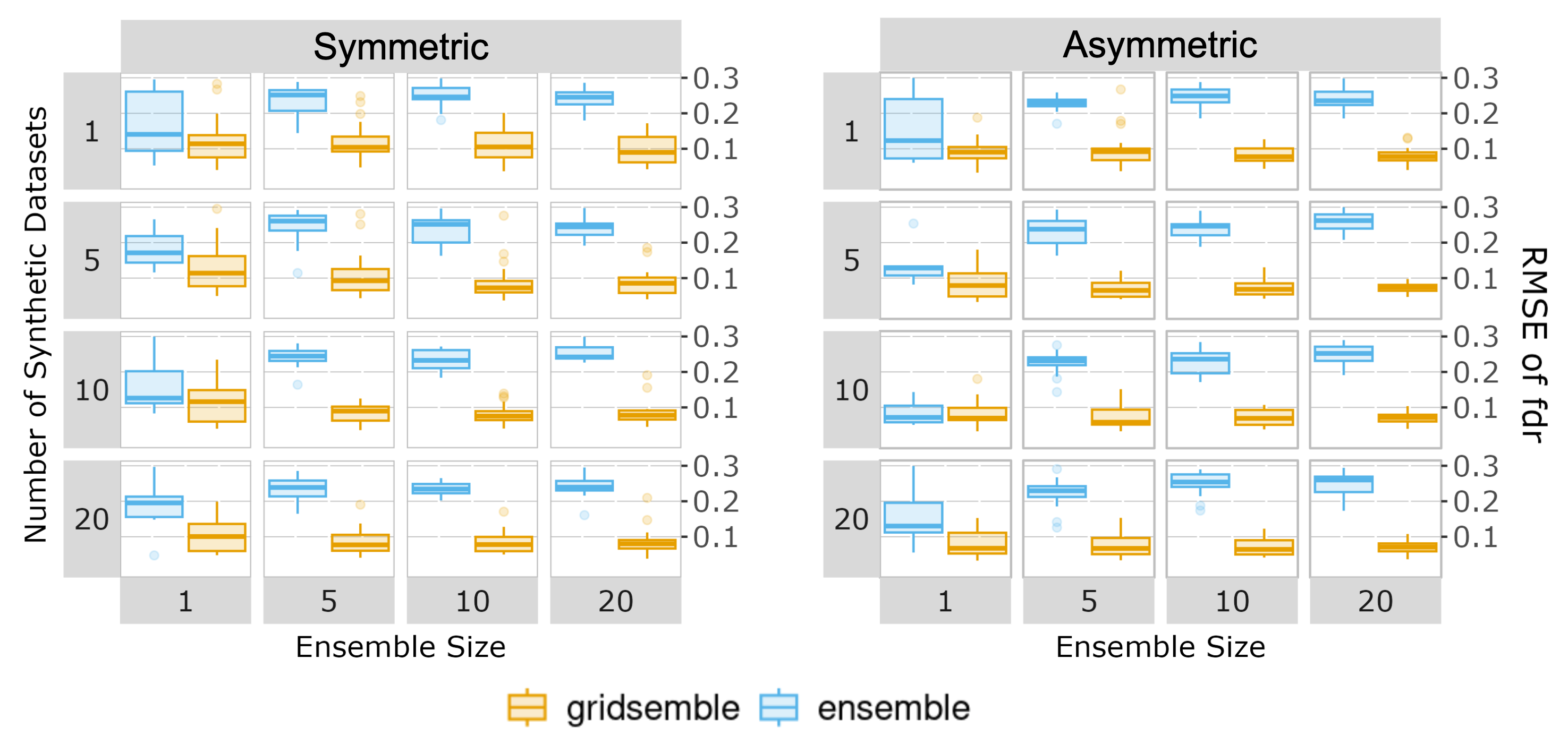
Figure 3: Comparing gridsemble to ensemble for varying ensemble size and number of synthetic datasets. Each box plot shows RMSE of fdr over 200 repetitions across the symmetric (left) and asymmetric (right) simulation studies. Key results include the improvement of gridsemble with increased number of synthetic datasets and with increased ensemble size, as well a plateau in the performance of gridsemble at 10 synthetic datasets and an ensemble size of 10.

7.4.2 Choosing $\mathbf{N}$ and $\mathbf{m}$

Computational power and time requirements increase with the number of synthetic datasets, $N$, and model size increases with ensemble size, $m$. To see the effects of these values on performance and determine optimal values of $N$ and $m$, we compare our new methods gridsemble and ensemble with varying number of synthetic datasets and ensemble sizes on the symmetric and asymmetric simulation studies (Figure 3).

In both studies, gridsemble improves as ensemble size increases and as the number of synthetic datasets increases. ensemble is unchanged by the number of synthetic datasets and performs worse as ensemble size increases. Around 10 synthetic datasets and an ensemble size of 10, the performance of gridsemble seems to plateau. Weighing the considerations of model size and computational requirements with these results, we move forward with 10 synthetic datasets and an ensemble size of 10, though these can be user-specified with our R package.

7.5 Statistical Properties of the Gridsemble Estimator

7.5.1 Bias

In this section, we derive an upper bound for the absolute bias of our estimator of the objective. As before, let the subscript $W$ refer to our working model with marginal density $f_{W}(u)$ while $\mathcal{P}$ refers to the real (unknown) data generating model with marginal density $f(u)$.

All synthetic datasets are drawn from the same working model, thus all $L(\widehat{\mathbf{fdr}}_{\theta}(\mathbf{u}^{n}),\mathbf{fdr}^{n})$ have the same expectation for a given $\theta$. We assume that $L(\widehat{\mathbf{fdr}}_{\theta}(\mathbf{u}),\mathbf{fdr})=\frac{1}{I}\sum_{i=1}^{I}L(\hbox{fdr}_{\theta}(u_{i}),\hbox{fdr}_{i})$.

$$\mathcal{L}(\theta) =E_{\mathcal{P}}\left[L(\widehat{\mathbf{fdr}}_{\theta}(\mathbf{u}),\mathbf{fdr})\right]=E_{\mathcal{P}}\left[L(\hbox{fdr}_{\theta}(u),\hbox{fdr})\right]$$ (14)

$$E\left[\widehat{\mathcal{L}}(\theta)\right] =E_{W}[L(\widehat{\mathbf{fdr}}_{\theta}(\mathbf{u}),\mathbf{fdr})]=E_{W}\left[L(\widehat{\hbox{fdr}}_{\theta}(u),\hbox{fdr})\right]=E_{\mathcal{P}}\left[\frac{f_{W}(u)}{f(u)}L(\widehat{\hbox{fdr}}_{\theta}(u),\hbox{fdr})\right]$$ (15)

$$\text{Bias}\left[\widehat{\mathcal{L}}(\theta)\right] =E\left[\widehat{\mathcal{L}}(\theta)\right]-\mathcal{L}(\theta)=E_{\mathcal{P}}\left[L(\widehat{\hbox{fdr}}_{\theta}(u),\hbox{fdr})\left(\frac{f_{W}(u)}{f(u)}-1\right)\right]$$ (16)

Equation 15 utilizes the fact that the working model has the same support as $\mathcal{P}$. We can immediately recognize that if our working model is equivalent to the real data model, then $\frac{f_{W}(u)}{f(u)}=1$ and the estimator is unbiased for the objective. Otherwise, the Cauchy-Schwartz inequality can be used to put an upper bound on absolute bias

$$\big{|}\mbox{Bias}\big{[} \widehat{\mathcal{L}}(\theta)\big{]}\big{|}\leq\Big{(}\underbrace{E_{\mathcal{P}}\Big{[}\Big{(}\frac{f_{W}(u)}{f(u)}-1\Big{)}^{2}\Big{]}}_{(1)} \underbrace{E_{\mathcal{P}}\Big{[}L\Big{(}\widehat{\hbox{fdr}}_{\theta}(u),\hbox{fdr}\Big{)}^{2}\Big{]}}_{(2)}\Big{)}^{1/2}$$ (17)

where (1) $=\mbox{Div}_{\chi^{2}}(f_{W}(u)||f(u))$ and (2) $=\mbox{Var}_{\mathcal{P}}\left[L(\widehat{\hbox{fdr}}_{\theta}(u),\hbox{fdr})\right]+\mathcal{L}(\theta)^{2}$.

This upper bound increases with (1) the Pearson $\chi^{2}$-divergence between the real and working marginal distributions and (2) the variance of the loss under the real data distribution plus the true objective squared.

7.5.2 Variance

In this section, we look at the variance of our estimate of the objective. Synthetic datasets are independent from one another and draws within each synthetic dataset are independent. Again, all synthetic datasets are drawn from the same working distribution.

Var $$\left[\hat{\mathcal{L}}(\theta)\right]=\frac{1}{N^{2}}\sum_{n=1}^{N}\mbox{Var}_{W}\left[L(\widehat{\mathbf{fdr}}_{\theta}(\mathbf{u}^{n}),\mathbf{fdr}^{n})\right]$$ (18)

$$=\frac{1}{N}\mbox{Var}_{W}\left[L(\widehat{\mathbf{fdr}}_{\theta}(\mathbf{u}),\mathbf{fdr})\right]$$

The variance of our estimator increases with the variance of the loss under the working model.

	Method	Brier Score	RMSE	PR AUC	ROC AUC
Symmetric	gridsemble	0.064	0.079	0.992	0.966
	grid	0.068	0.101	0.991	0.962
	ensemble	0.127	0.266	0.991	0.963
	ensemble_all	0.132	0.273	0.992	0.966
	locfdr	0.096	0.197	0.941	0.870
	fdrtool	0.110	0.231	0.916	0.810
	qvalue	0.462	0.636	0.990	0.955
Asymmetric	gridsemble	0.032	0.069	0.998	0.989
	grid	0.034	0.083	0.998	0.988
	ensemble	0.095	0.262	0.998	0.986
	ensemble_all	0.091	0.255	0.998	0.989
	locfdr	0.034	0.089	0.993	0.976
	fdrtool	0.063	0.193	0.955	0.858
	qvalue	0.313	0.536	0.998	0.986
Curated Ovarian Data-Based	gridsemble	0.066	0.050	0.966	0.919
	grid	0.067	0.048	0.964	0.913
	ensemble	0.074	0.163	0.970	0.925
	ensemble_all	0.081	0.171	0.972	0.929
	locfdr	0.061	0.058	0.968	0.924
	fdrtool	0.107	0.196	0.903	0.776
	qvalue	0.067	0.047	0.965	0.913

Table 1: Simulation study results showing median metrics of gridsemble and each of the sub-models grid, ensemble, and ensemble_all versus each of the baselines locfdr, fdrtool, and qvalue. Best value of each metric in each study is highlighted. Companion to Figure 1 recording median values from each boxplot. Used to discuss difference in median metrics in Results.

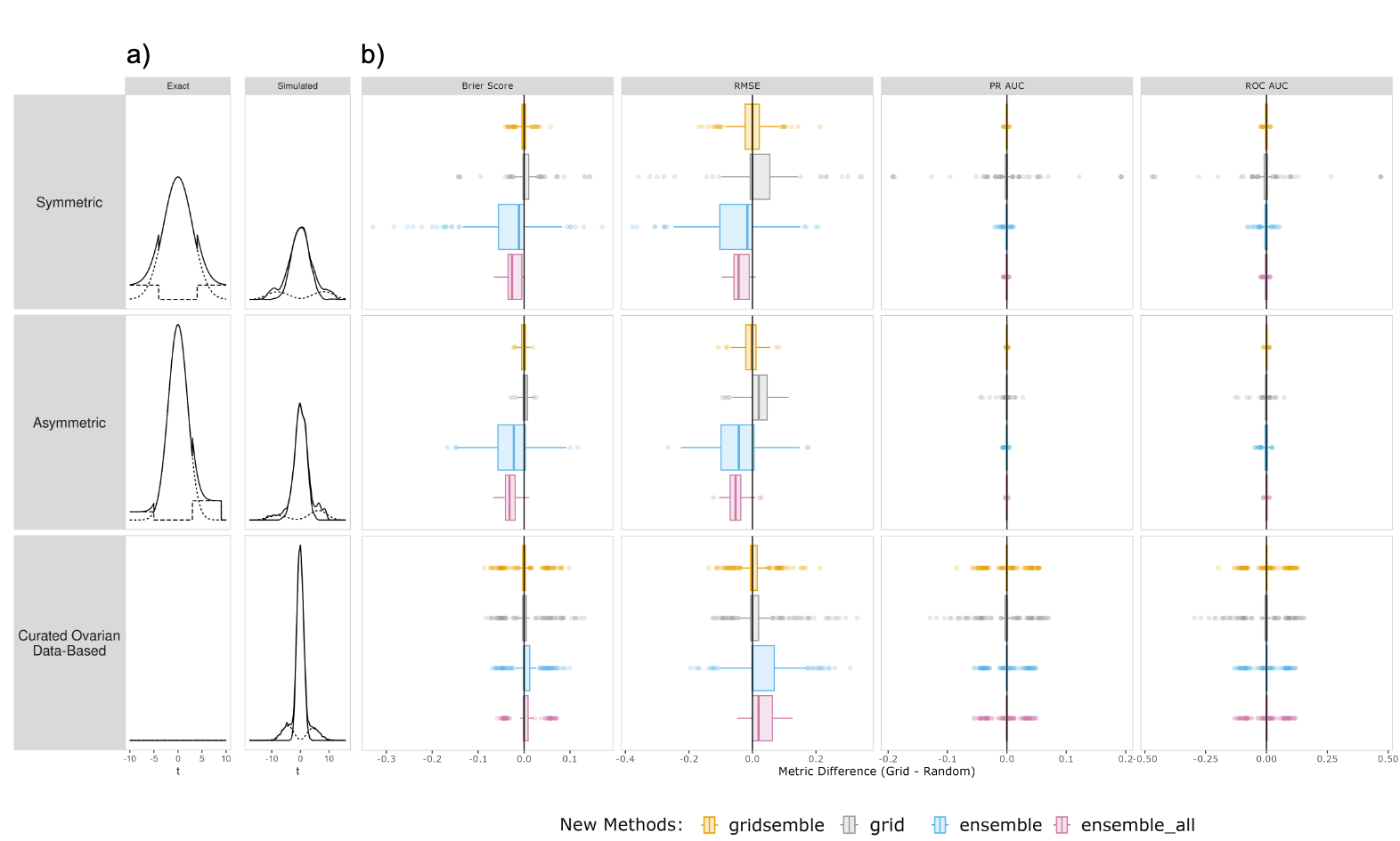
Figure 1: Simulation study results comparing equally-spaced vs random grid. a) Simulation study distributions. b) Simulation study results of gridsemble and each of the sub-models grid, ensemble, and ensemble_all using an equally-spaced grid versus randomly selected parameter values (i.e., grid search versus random search). Plotted are the pairwise differences in metrics (grid search - random search).

	gridsemble	locfdr	fdrtool	qvalue
ROC AUC	0.944	0.943	0.849	0.899
PR AUC	0.962	0.962	0.856	0.905
Brier Score	0.112	0.135	0.132	0.104
MSE Fdr	0.014	0.028	0.007	0.005
$\hat{\pi}_{0}$	0.77	0.59	0.72	1
Standard 0.2 Cutoff
cutoff $c^{(1)}$	0.2	0.2	0.2	0.2
FDR	0.021	0.176	0.100	0.082
Sensitivity	0.266	0.899	0.708	0.638
True Discoveries	518	1747	1377	1240
False Discoveries	11	372	153	110
$\pi_{0}$-Based Cutoff
cutoff $c^{(2)}$	0.74	0.13	1	1
FDR	0.150	0.150	0.638	0.638
Sensitivity	0.850	0.850	0.999	1
True Discoveries	1652	1652	1943	1944
False Discoveries	292	292	3426	03426
$\hat{\pi}_{0}$-Based Cutoff
cutoff $c^{(2)}$	0.60	0.23	0.12	0
FDR	0.073	0.197	0.096	0
Sensitivity	0.599	0.908	0.705	0.001
True Discoveries	1165	1765	1370	2
False Discoveries	92	434	146	0

Table 2: Results on experimental application comparing gridsemble to each of the baseline methods. Best values of each metric are shaded. The top four metrics evaluate estimated false discovery rates. $\hat{\pi}_{0}$ should be compared to the true value $\pi_{0}=0.638$. Classification metrics show the downstream utility of estimated fdr values in classifying tests as null (small fdr) or not-null (large fdr). FDR is global false discovery rate, the proportion of discovered tests that are actually null. Recall, or sensitivity, is the proportion of non-null tests that were correctly discovered. Classification 1 uses a constant cutoff of 0.2. Classification 2 uses a different cutoff for each method such that $\hat{\pi}_{0}$ proportion of tests are classified as null.

References

- Dudoit et al. [2003] Sandrine Dudoit, Juliet Popper Shaffer, and Jennifer C. Boldrick. Multiple hypothesis testing in microarray experiments. Statistical Science, 18(1):71–103, 2003. doi:10.1214/ss/1056397487.
- Farcomeni [2008] Alessio Farcomeni. A review of modern multiple hypothesis testing, with particular attention to the false discovery proportion. Statistical methods in medical research, 17(4):347–388, 2008. doi:10.1177/0962280206079046.
- Committee on Reproducibility and Replicability in Science [2019] Committee on Reproducibility and Replicability in Science. Reproducibility and Replicability in Science. National Academies Press, Washington, D.C., 2019. ISBN 978-0-309-48616-3. doi:10.17226/25303.
- Tukey [1953] John Wilder Tukey. The problem of multiple comparisons. Multiple comparisons, 1953.
- Tukey [1991] John W Wilder Tukey. The Philosophy of Multiple Comparisons. Statistical science, pages 100–116, 1991. doi:10.1214/ss/1177011945.
- Benjamini and Hochberg [1995] Y. Benjamini and Y. Hochberg. Controlling the false discovery rate: A practical and powerful approach to multiple testing. Journal of the Royal Statistical Society Series B, 57:289–300, 1995. doi:10.1111/j.2517-6161.1995.tb02031.x.
- Efron et al. [2001] Bradley Efron, Robert Tibshirani, John D Storey, and Virginia Tusher. Empirical bayes analysis of a microarray experiment. Journal of the American Statistical Association, 96:456:1151–1160, 2001. doi:10.1198/016214501753382129.
- Efron et al. [2015] Bradley Efron, Brit Turnbull, Balasubramanian Narasimhan, and Korbinian Strimmer. locfdr: Computes Local False Discovery Rates, 2015. R package version 1.1-8.
- Klaus and Strimmer [2021] Bernd Klaus and Korbinian Strimmer. fdrtool: Estimation of (Local) False Discovery Rates and Higher Criticism, 2021. R package version 1.2.17.
- Strimmer [2008] Korbinian Strimmer. fdrtool: a versatile r package for estimating local and tail area-based false discovery rates. Bioinformatics, 24:1461–1462, 2008.
- Storey et al. [2015] John Storey, Andrew Bass, Alan Dabney, and David Robinson. qvalue: Q-value estimation for false discovery rate control, 2015. R package version 2.28.0.
- Efron and Tibshirani [2002] Bradley Efron and Robert Tibshirani. Empirical bayes methods and false discovery rates for microarrays. Genetic Epidemiology, 23(1)(1):70–86, June 2002. doi:10.1002/gepi.1124.
- Stephens [2016-10] Matthew Stephens. False discovery rates: a new deal. Biostatistics (Oxford, England), 18(2):275–294, April 2016-10. ISSN 1465-4644. doi:10.1093/biostatistics/kxw041.
- Müller et al. [2007] Peter Müller, Giovanni Parmigiani, and Kenneth Rice. FDR and Bayesian multiple comparisons rules. In Bayesian Statistics 8. Oxford University Press, 2007. doi:10.1093/oso/9780199214655.003.0014.
- Yu and Zhu [2020] Tong Yu and Hong Zhu. Hyper-parameter optimization: A review of algorithms and applications. arXiv preprint arXiv:2003.05689, 2020. doi:10.48550/arXiv.2003.05689.
- Kuhn et al. [2013] Max Kuhn, Kjell Johnson, et al. Applied predictive modeling, volume 26. Springer, 2013. doi:10.1007/978-1-4614-6849-3.
- Nomura and Saito [2021] Masahiro Nomura and Yuta Saito. Efficient hyperparameter optimization under multi-source covariate shift. CIKM, 2021. doi:10.1145/3459637.3482336.
- Efron [1982] Bradley Efron. The jackknife, the bootstrap and other resampling plans. SIAM, 1982.
- Kohavi et al. [1995] Ron Kohavi et al. A study of cross-validation and bootstrap for accuracy estimation and model selection. In Ijcai, volume 14, pages 1137–1145. Montreal, Canada, 1995.
- Dong et al. [2020] Xibin Dong, Zhiwen Yu, Wenming Cao, Yifan Shi, and Qianli Ma. A survey on ensemble learning. Frontiers of Computer Science, 14(2):241–258, 2020. ISSN 2095-2236. doi:10.1007/s11704-019-8208-z.
- Madigan and Raftery [1994] David Madigan and Adrian E. Raftery. Model selection and accounting for model uncertainty in graphical models using occam’s window. Journal of the American Statistical Association, 89(428):1535–1546, 1994. ISSN 01621459. doi:10.1080/01621459.1994.10476894.
- Ryu et al. [2002] Byungwoo Ryu, Jessa Jones, Natalie J Blades, Giovanni Parmigiani, Michael A Hollingsworth, Ralph H Hruban, and Scott E Kern. Relationships and differentially expressed genes among pancreatic cancers examined by large-scale serial analysis of gene expression. Cancer research, 62(3):819–826, 2002.
- Cui and Churchill [2003] Xiangqin Cui and Gary A Churchill. Statistical tests for differential expression in cDNA microarray experiments. Genome biology, 4:1–10, 2003. doi:10.1186/gb-2003-4-4-210.
- Lu et al. [2005] Jun Lu, John K Tomfohr, and Thomas B Kepler. Identifying differential expression in multiple sage libraries: an overdispersed log-linear model approach. BMC bioinformatics, 6:1–14, 2005. doi:10.1186/1471-2105-6-165.
- Robinson and Smyth [2007] Mark D Robinson and Gordon K Smyth. Moderated statistical tests for assessing differences in tag abundance. Bioinformatics, 23(21):2881–2887, 2007. doi:10.1093/bioinformatics/btm453.
- Chen et al. [2020] Yunshun Chen, Davis McCarthy, Matthew Ritchie, Mark Robinson, Gordon Smyth, and E Hall. edgeR: differential analysis of sequence read count data user’s guide. R Package, pages 1–121, 2020.
- Varet et al. [2016] Hugo Varet, Loraine Brillet-Guéguen, Jean-Yves Coppée, and Marie-Agnès Dillies. Sartools: a deseq2-and edger-based r pipeline for comprehensive differential analysis of rna-seq data. PloS one, 11(6):e0157022, 2016. doi:10.1371/journal.pone.0157022.
- Rossell and Telesca [2017] David Rossell and Donatello Telesca. Non-local priors for high-dimensional estimation. Journal of the American Statistical Association, 112:254–265, 2017. doi:10.1080/01621459.2015.1130634.
- Dempster et al. [1977] Arthur P Dempster, Nan M Laird, and Donald B Rubin. Maximum likelihood from incomplete data via the em algorithm. Journal of the royal statistical society: series B (methodological), 39(1):1–22, 1977. doi:10.1111/j.2517-6161.1977.tb01600.x.
- Ganzfried et al. [2013] BF Ganzfried, M Riester, B Haibe-Kains, T Risch, S Tyekucheva I Jazic, XV Wang, M Ahmadifar, M Birrer, G Parmigiani, C Huttenhower, and L Waldron. curatedOvarianData: Clinically annotated data for the ovarian cancer transcriptome. 2013. doi:10.1093/database/bat013.
- Zhu et al. [2010] Q. Zhu, J.C. Miecznikowski, and M.S. Halfon. Preferred analysis methods for affymetrix genechips. II. an expanded, balanced, wholly-defined spike-in dataset. BMC Bioinformatics, 11:285, 2010. doi:https://doi.org/10.1186/1471-2105-11-285.
- Irizarry et al. [2003] Rafael A Irizarry, Bridget Hobbs, Francois Collin, Yasmin D Beazer-Barclay, Kristen J Antonellis, Uwe Scherf, and Terence P Speed. Exploration, normalization, and summaries of high density oligonucleotide array probe level data. Biostatistics, 4(2):249–264, 2003. doi:10.1093/biostatistics/4.2.249.
- Efron [2007] Bradley Efron. Size, power and false discovery rates. The Annals of Statistics, 35:1351–1377, 2007. doi:10.1214/009053606000001460.
- Steyerberg and Vergouwe [2014] Ewout W Steyerberg and Yvonne Vergouwe. Towards better clinical prediction models: seven steps for development and an ABCD for validation. European heart journal, 35(29):1925–1931, 2014. doi:10.1093/eurheartj/ehu207.
- Garrido-Merchán and Hernández-Lobato [2020] Eduardo C Garrido-Merchán and Daniel Hernández-Lobato. Dealing with categorical and integer-valued variables in bayesian optimization with gaussian processes. Neurocomputing, 380:20–35, 2020. doi:https://doi.org/10.1016.
Supplementary Materials for