Threshold Quantum State Tomography

Abstract

Quantum state tomography (QST) aims at reconstructing the state of a quantum system. However in conventional QST the number of measurements scales exponentially with the number of qubits. Here we propose a QST protocol, in which the introduction of a threshold allows one to drastically reduce the number of measurements required for the reconstruction of the state density matrix without compromising the result accuracy. In addition, one can also use the same approach to reconstruct an approximated density matrix depending on the available resources. We experimentally demonstrate this protocol by performing the tomography of states up to 7 qubits. We show that our approach can lead to the same accuracy of QST even when the number of measurements is reduced by more than two orders of magnitudes.

I Introduction

In the last few years, the race for quantum technologies has favoured the realization of large and complex quantum states in various platforms, including superconducting Cao et al. (2023), atomic Häffner et al. (2005); Monz et al. (2011), and photonic systems Wang et al. (2016); Zhang et al. (2019); Gao et al. (2010); Agnew et al. (2011); Reimer et al. (2019); Madsen et al. (2022). Such advances are an important resource for the implementation of useful quantum computers and an extraordinary opportunity for fundamental studies in quantum mechanics.

Ideally, one would like to know the complete state of a quantum system, for this is sufficient to compute the value of any other observable. However, as the dimension of the quantum system increases, this task is not trivial at all. For example, consider quantum state tomography (QST) James et al. (2001), which is arguably the most famous approach for quantum state reconstruction. The idea is to obtain the density matrix of the system from the measurements of a set of observables on a large enough ensemble of identical copies of the state. This method is general and does not make any a priori hypothesis on the state. However, a system composed of $n$ qudits requires determining the expectation value of at least $d^{2n}$ observables, that is the number of independent entries of the density matrix. Such an exponential growth of the number of measurements with the number of qudits can make the experimental implementation of QST unfeasible even for just three or four qudits, depending on the quantum system under investigation.

Over the years, strategies have been developed to decrease the number of required measurements, usually by leveraging certain assumptions about the state or the anticipated outcome. For example, the efficiency of compressed sensing QST depends on the rank of the density matrix, with the state characterization done via a certain number of random Pauli measurements Gross et al. (2010). Further improvements of this approach have reduced the number of necessary measurement sets significantly Ahn et al. (2019a, b). In QST via reduced density matrices, one requires the state to be uniquely determined by local reduced density matrices or the hypothesis that the global state is pure Xin et al. (2017). In Bayesian QST, one defines conditional probabilities starting from measurement results and a suitable a priori distribution over the space of possible states Derka et al. (1997). In self-guided QST one addresses tomography through optimization rather than estimation, iteratively learning the quantum state by treating tomography as a projection measurement optimization problem Ferrie (2014); Chapman et al. (2016); Rambach et al. (2021).

Figure 1: Pictorial representation of the tQST process. (1) Measurement of the diagonal terms $\rho_{ii}$; (2) Choice of the threshold $t$. The choice of $t$ resembles that of positioning the bar in a limbo competition. If the bar is very low ($t\ll 1$), a successful performance will certainly be spectacular. However, if the bar is too low, the dance may be prohibitive even for a most skilled athlete. This is the situation of conventional QST when the number of measurements to be performed is unreasonable. On the contrary, for a sufficiently high bar, even a beginner may be able to dance, but the result may not be particularly noteworthy. (3) Construction and measurement of the observable associated with the off-diagonal terms; (4) Reconstruction of the density matrix; we plot the absolute values of the matrix elements colored by their phase as indicated by the color bar.

Other strategies avoid the reconstruction of the density matrix by focusing only on some relevant information about the state. For instance, in shadow tomography, one can estimate the value of a large number of observables with a few copies of the unknown state Aaronson (2018); Huang et al. (2020); Struchalin et al. (2021). Finally, quantum witnesses are useful to verify some crucial properties of a quantum state, such as its degree of entanglement and the kind of quantum correlation Zhu et al. (2010). While these last two approaches are extremely useful and applicable to states of large dimensions, it is somewhat disappointing that, after all the efforts to implement a state, one cannot look at it as a whole.

In this work, we introduce threshold Quantum State Tomography (tQST), a protocol that allows one to reconstruct the density matrix of a quantum state, even of large dimension, by allowing an efficient trade-off between the number of measurements and the accuracy of the state reconstruction through the presence of a threshold parameter. We show that tQST can drastically reduce the resources required for state reconstruction, but it can also be used to obtain an approximated density matrix by further reducing the number of measurements and the experimental efforts. The protocol can be applied to any quantum system and does not make any assumption about the state to be characterized. First, we outline the tQST procedure and discuss its implementations in the case of $n$-qubits. Second, we experimentally verify the protocol by performing tQST on systems up to 7 qubits with the IBMQ platform and compare the results with conventional QST. Finally, we draw our conclusions.

II Results

II.1 The threshold quantum state tomography protocol

In conventional QST, the number of measurements required to reconstruct the density matrix is uniquely determined by its dimension James et al. (2001). Specifically, a system of $n$ qubits requires at least $4^{n}$ measurements, that is the number of independent parameters of the state density matrix. These measurements can be performed in an arbitrary sequence, and the results are finally combined to obtain the state density matrix (through maximum likelihood estimation or other approaches Kaznady and James (2009); Lukens et al. (2020)).

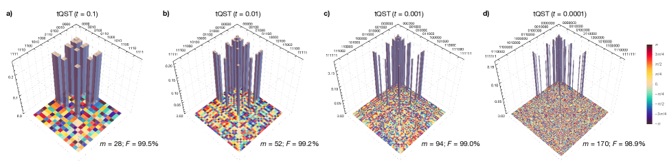
Figure 2: Reconstruction of the density matrix of a W state via tQST. We consider different numbers of qubits and threshold values: a) 4 qubits, $t=0.1$ b) 5 qubits, $t=0.01$, c) 6 qubits, $t=0.001$, and d) 7 qubits, $t=0.0001$. For each case, we indicate the number of measurements used and the fidelity with the corresponding target state.

Here, we start by observing that any element $\rho_{ij}$ of a physical density matrix $\rho$ must satisfy $|\rho_{ij}|\leq\sqrt{\rho_{ii}\rho_{jj}}$. This inequality follows from the fundamental properties of $\rho$ of being unit-trace, Hermitian, and positively defined Nielsen and Chuang (2010). Thus, measuring the diagonal elements of the density matrix (i.e., projecting on the states of the computational basis) provides some information on the off-diagonal terms. Indeed, if $\rho_{ii}$ is found to be zero, then one can immediately set to zero all the elements of the $i$-th row and column of $\rho$. Similarly, if $\rho_{ii}$ and $\rho_{jj}$ are different from zero but small compared to the other diagonal elements, one knows that the modulus of $\rho_{ij}$ will be small too.

These considerations are at the basis of tQST, whose protocol is illustrated in Fig. 1. First, one measures the diagonal elements $\{\rho_{ii}\}$ of the density matrix, which are directly accessible by projecting on the chosen computational basis. Second, one chooses a threshold $t$ and, by exploiting the information on $\{\rho_{ii}\}$, identifies those $\rho_{ij}$ for which $\sqrt{\rho_{ii}\rho_{jj}}\geq t$. Third, one constructs a proper set of observables associated with these $\rho_{ij}$ (see Methods) and performs only those measurements. Finally, one uses these results to reconstruct the density matrix, for example, using a maximum-likelihood estimation.

In tQST, the information achieved by measuring the diagonal terms of $\rho$ is immediately used to decide the subsequent measurements to be performed, by choosing to neglect the terms of $\rho$ that in modulus are smaller than a certain threshold. Unlike conventional QST, the resources necessary to reconstruct the state are not uniquely determined by the dimension of the quantum system but can be controlled with the threshold $t$. For example, if one sets $t=0$, all the elements of $\rho$ are considered, and the protocol reduces to conventional QST. On the contrary, for $t>0$, the protocol may require fewer measurements than those needed with conventional QST and, in any case, no more than them. Importantly, one does not make any a priori hypothesis on the state or the result of the characterization. It should be noted that unlike adaptive approaches Ahn et al. (2019a, b), in which the necessary measurement sets cannot be known a priori, for each one is chosen based on the outcomes of the previous measurement set, in tQST the projectors can all be determined once the system is measured in the chosen computational basis.

The threshold $t$ determines the amount of information one is willing to trade in exchange for fewer measurements. This has several consequences. First, one may be able to reconstruct the entire density matrix of a large state by reducing the amount of measurements to a level compatible with the available experimental resources. Second, fewer measurements can give a significant advantage in terms of storing and handling experimental data. Third, one may be able to avoid useless measurements and increase the integration time for the remaining measurements, leading to an improvement of the signal-to-noise ratio. The amount of information obtainable in the characterization of a quantum state is always limited, for example by noise or the finite precision of the experimental setup. Such experimental constraints de facto bound the accuracy with which $\rho$ can be determined, even for traditional QST. Thus, although one may naively expect that reducing the number of measurements will decrease the quality of the results, as we shall see in the following, a wise choice of $t$ can still guarantee reaching the best achievable result but by implementing fewer resources.

In Fig. 2 we show the simulated reconstruction of the density matrix via tQST with maximum likelihood estimation of several W states for different numbers of qubits ranging from 4 to 7 Dür et al. (2000). Even for the case of 7 qubits, in which traditional QST would have required 16,384 measurements, one can reconstruct $\rho$ with a fidelity of about 99% with the target state by implementing only 170 measurements. We stress that here the dramatic reduction of measurements is not simply given by the choice of a particular state, but rather by the employed computational basis, which affects the final state representation. As in compressed sensing tomography or similar approaches, sparse matrices are usually easier to reconstruct, because most of the information is contained in fewer elements of the density matrix. Yet, for sparse matrices the advantage of tQST can be significantly larger than with other approaches. Take for example the 7-qubit state reconstructed in Ref. Riofrio et al. (2017) via compressed sensing QST, in which the characterization required 16,256 projective measurements. While this number is significantly smaller than $6^{n}$, which is the number of observables of the typical tomographically overcomplete set, this is still 99% of the $4^{n}$ observables that are strictly necessary James et al. (2001). On the contrary, the very same state could be reconstructed via tQST by performing only 184 measurements, which is about 1% of those required by compressed sensing (see Supplementary Material). We stress that tQST can also be applied to matrices that are not sparse, where the threshold $t$ will determine both the number of measurements and the accuracy of the results.

As shown in Fig. 2, a notable feature of tQST is that a significant reduction in the number of measurements does not necessarily lead to large errors in the reconstruction of the density matrix. However, this feature is strongly dependent on the state representation. More in general, one may be interested in using tQST because the available resources are simply not enough to implement the traditional QST. In this case, it is important to have an estimate of the largest error that is associated with the threshold choice. Specifically, given $\{\rho_{ii}\}$ and $t$, one can estimate a lower bound for the fidelity of the state $\rho$ obtained via tQST with an expected target state $\rho_{t}$ (see Methods):

$$F_{\mathrm{bound}}(\rho,\rho_{t},t)=\left(1-\sqrt{r(\rho_{t})\sum_{(i,j)\in\mathcal{C}_{t}}\rho_{ii}\rho_{jj}}\right)^{2},$$ (1)

where $r\left(\rho_{t}\right)$ is the rank of $\rho_{t}$ and $\mathcal{C}_{t}$ defines the ensemble of $\rho_{ij}$ that are below threshold (i.e., $\mathcal{C}_{t}=\left\{\left(i,j\right)\mid\sqrt{\rho_{ii}\rho_{jj}}<t\right\}$). We stress that in some cases this can be a quite conservative lower bound but still useful to verify whether a resulting low fidelity depends on the choice of an excessively high threshold, or rather a real dissimilarity between $\rho$ and the target state.

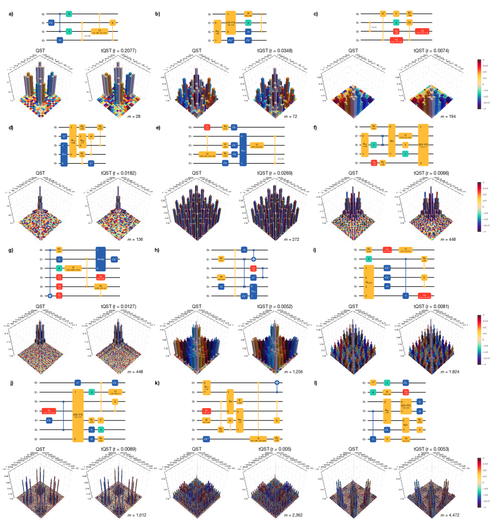
Figure 3: tQST on random circuits implemented in a IBMQ processor. a), b), c): 4-qubit states generated with the shown circuits with a diagonal filling of 25% , 50%, and 75%, respectiv4ely. d) - l): same as before, with 5, 6, and 7 qubits.

Figure 4: Quantitative comparison between the reconstructed QST and tQST density matrices of the random circuits illustrated in Fig. 3. a) Comparison of QST and tQST density matrix fidelities. The red line represents the tQST fidelity bound corresponding to the specified circuit threshold. b) Scaling of the required measurements with the number of qubits for both QST and tQST reconstructions.

II.2 Implementation on an IBMQ processor

We experimentally demonstrate tQST by using the IBMQ processor lagos Qiskit contributors (2023); Kanazawa et al. (2023), which allows one to prepare states with up to 7 superconducting qubits. In our implementation, each time we program the system to generate a target quantum state by constructing the corresponding quantum circuit (Methods, Sec. IV.5). We first reconstruct the state density matrix by performing conventional QST as implemented by IBMQ, which uses linear inversion on the outcomes of an overcomplete set of $6^{n}$ observables. This process generally yields a non-positive reconstructed state, which is subsequently rescaled to be positively defined using the method outlined in Smolin et al. (2012) (Methods, Sec. IV.5). We then reconstruct the same state by using tQST, where the threshold $t$ is chosen by considering the typical signal-to-noise ratio (SNR) of the system to avoid unnecessary measurements (Methods, Sec. IV.2). In this case, we use a maximum likelihood estimation to obtain the (positive-definite) density matrix from the measured expectation values (Methods, Sec. IV.4). To compare the results we compute the fidelities between the target state and the reconstructed ones, and also that between the two reconstructed states.

In our analysis, we generated several random states and sorted them according to the diagonal filling, i.e., the percentage of expected non-vanishing diagonal elements. In Fig. 3 we show representative results for filling percentages of 25% (a,d,g,j), 50% (b,e,h,k), and 75% (c,f,i,l) for a number of qubits ranging from 4 (a,b,c) to 7 (j,k,l). Each panel of the figure shows the circuit to generate the state, the density matrix reconstructed with conventional QST, and the one obtained with tQST. In this last case, we also report the value of the threshold $t$ and the corresponding number of measurements used in the reconstruction. Since we choose $t$ according to the typical SNR of the system, such a number is also related to the sparsity of the state representation. For the cases of 4, 5, and 6 qubits, we observe up to a 100-fold reduction in the number of required measurements compared to IBMQ-QST. For the case of 7 qubits, such reduction is $\sim 300$ for the case of Fig. 3j.

As evident from the state representation, despite the significant difference in the number of measurements, the state reconstructed with IBMQ-QST and tQST are very similar. A more quantitative analysis is obtained by calculating the fidelity between the two reconstructed states, which in all cases is about 90% or above, as shown in Fig. 4. The same figure also reports the fidelity of the tQST-reconstructed state with the target one. Remarkably, this is always slightly higher or comparable to the fidelity between the IBMQ-QST reconstructed state and the target one. Thus no advantage is obtained with IBMQ-QST by performing more measurements than those set by the threshold in tQST. This suggests that when the threshold is determined by the SNR of the system, the tQST protocol can extract all the amount of information accessible with conventional QST, yet with a smaller number of measurements.

The IBMQ processor lagos limits our analysis to 7 qubits. Yet, it is interesting to further investigate the performance of tQST by extrapolating the analysis to a larger number of qubits. In this analysis we considered simulated data with a SNR analogous to that of the IBMQ system and followed the same strategy for the threshold choice. We considered the case of W states and increased the number of qubits up to 14, limited now only by our hardware. In Table 1 we report the number of qubits, the threshold $t$, the number of measurements, and the fidelity with respect to the target state. In all the cases we obtained fidelities exceeding 90%. We stress that in the cases of 14 qubits, the 16,556 measurements required by tQST make the reconstruction in principle experimentally accessible today. On the contrary, conventional QST would necessitate at least $4^{14}=268,435,456$ measurements that, at the moment, appear as a prohibitive number.

Qubits	Threshold ($t$)	Measures	Fidelity
8	0.053	312	91.5%
9	0.047	584	91.9%
10	0.042	1,114	91.2%
11	0.038	2,158	91.4%
12	0.035	4,228	91.4%
13	0.032	8,348	91.3%
14	0.030	16,556	91.3%

Table 1: tQST reconstruction of a W state from synthetic data where an ad-hoc noise similar to the one observed in Ref. Häffner et al. (2005) has been introduced. The number of the needed off-diagonal measures for the state reconstruction scales as $n^{2}-n$ with the number of qubits, and therefore it is subdominant with respect to the number of diagonal measurements ($2^{n}$) necessary for the determination of the threshold.

III Discussion

We have proposed and implemented a protocol for QST that allows one to reconstruct the density matrix of any quantum state with a number of measurements that can be considerably smaller than that required by conventional QST. Such an approach does not make any a priori hypothesis on the state and employs a threshold $t$ to control the amount of information used in the state reconstruction. The presence of such a threshold allows one to trade the minimum fidelity with which the state can be reconstructed with the amount of resources to perform the characterization, thus reducing the number of measurements significantly. In addition, the threshold can be set to take into account the experimental limitations that may lead to unnecessary measurements. Our protocol was implemented on the IBMQ system lagos to characterize random states up to 7 qubits. In all the considered cases the fidelity achieved with tQST was comparable (or slightly larger) than that obtained by using conventional QST but with a smaller amount of measurements (in some cases $\sim 300$ times smaller). This suggests that our protocol is able to efficiently access all the information that can be extracted from the system. Finally, by using synthetic data, we pushed the approach to our computational limit and performed the characterization of W states up to 14 qubits, reaching a fidelity larger than 90% with only $\sim 16,000$ expectation values, four orders of magnitudes less than what would be required by conventional QST.

Our protocol is a flexible and practical approach for the full characterization of large quantum systems, including those based on atoms or photons. For this reason, we believe that it will be particularly useful to the whole quantum community.

IV Methods

IV.1 $n$-qubit projectors

The real (respectively, imaginary) part of an off-diagonal element of a density matrix $\rho$, can be obtained from:

$$\rho^{\mathrm{re,im}}_{i,j}=\mathrm{tr}\left({\cal O}^{\mathrm{re,im}}_{ij}\rho\right),$$ (2)

where ${\cal O}^{\mathrm{re}}_{ij}$ (respectively, ${\cal O}^{\mathrm{im}}_{ij}$) is an operator with: $1/2$ (respectively, $i/2$) at the entry $ij$; $1/2$ (respectively, $-i/2$) at the entry $ji$; and zero otherwise. How to experimentally conduct a series of measurements corresponding to these operators remains unknown. Instead, one can explore a set of $4^{n}$ projectors, denoted as $P=\left|{\psi}\right\rangle\left\langle{\psi}\right|$, where $\left|{\psi}\right\rangle$ is separable ($\left|{\psi}\right\rangle=\otimes_{k}\left|{\phi_{k}}\right\rangle$). These projectors are then associated with the real or imaginary part of the matrix element $ij$ of the density matrix by ensuring that

$$P^{\mathrm{re,im}}_{ij}=\mathrm{min}_{P}\|{\cal O}^{\mathrm{re,im}}_{ij}-P\|_{2},$$ (3)

where $\|{\circ}\|_{2}$ represents the Frobenius norm.

A given set of projectors is said to be tomographically complete if there exists a unique set of scalars $a^{\mathrm{re,im}}_{K}$ (with $K=\{(ij\})$ a multi-index) such that the density matrix can be reconstructed, that is

$$\rho=\sum_{K}a^{\mathrm{re,im}}_{K}P^{\mathrm{re,im}}_{K}.$$ (4)

Equivalently, suppressing the “re” and “im” superindices, one gets

$$\mathrm{tr}\left(P_{L}^{\dagger}\rho\right)=\sum_{K}a_{K}\mathrm{tr}\left(P_{L}^{\dagger}P_{K}\right)=\sum_{K}M_{LK}a_{K}.$$ (5)

which means that the matrix $M_{LK}=\mathrm{tr}\left(P_{L}^{\dagger}P_{K}\right)=|\langle\psi_{L}|\psi_{K}\rangle|^{2}$ has to be invertible and the scalars $a_{K}$ are uniquely determined as $a_{K}=\left(M^{-1}\right)_{KL}\mathrm{tr}\left(P_{L}^{\dagger}\rho\right)$ James et al. (2001). Notice that, owing to the presence of equivalent minima in Eq. (3), it is not guaranteed that a complete set exists; however, if that is the case, then the matrix $M$ is positive definite.

We found that in the case of an $n$-qubit system, a tomographically complete set of projectors associated to the elements of a $n$-qubit density matrix can be obtained from the eigenvectors of the Pauli matrices. In the conventional polarization notation, these eigenvectors are:

$$\left|{H}\right\rangle;\! \left|{D}\right\rangle=\frac{1}{\sqrt{2}}\left(\left|{H}\right\rangle+\left|{V}\right\rangle\right); \left|{R}\right\rangle=\frac{1}{\sqrt{2}}\left(\left|{H}\right\rangle+i\left|{V}\right\rangle\right),$$

$$\left|{V}\right\rangle; \left|{A}\right\rangle=\frac{1}{\sqrt{2}}\left(\left|{H}\right\rangle-\left|{V}\right\rangle\right); \left|{L}\right\rangle=\frac{1}{\sqrt{2}}\left(\left|{H}\right\rangle-i\left|{V}\right\rangle\right).$$ (6)

In the 1-qubit case one possibility is: $P^{\mathrm{re}}_{11}=\left|{H}\right\rangle$; $P^{\mathrm{re}}_{22}=\left|{V}\right\rangle$; $P^{\mathrm{re}}_{12}=\left|{D}\right\rangle$; and $P^{\mathrm{im}}_{12}=\left|{R}\right\rangle$; or, in a more suggestive form

$$\pi_{1}\equiv\begin{bmatrix}\left|{H}\right\rangle&\left|{D}\right\rangle+i\left|{R}\right\rangle\\ 0&\left|{V}\right\rangle\end{bmatrix}.$$ (7)

This is a $2\times 2$ table structured in such a way that the projector associated with measuring the real or imaginary component of the element $\rho_{i,j}$ of the 1-qubit density matrix is given by the real or imaginary part of the entry $(i,j)$ in (7). For example, information on the imaginary part of $\rho_{1,2}$ is encoded in the matrix element $\left\langle{R}\right|\rho\left|{R}\right\rangle$. Entries with a value of “0” (which indeed acts as the zero element for the recursive operations below) do not need to be explicitly determined, as the density matrix is Hermitian. Consequently, we will assume, without loss of generality, that $j\geq i$ whenever we aim to determine $P_{ij}$.

A set of tomographically complete separable projectors for $n>1$ can be then constructed through the following recursion relation:

$$\pi_{n}=\begin{bmatrix}\left|{H}\right\rangle\pi_{n-1}&\left|{D}\right\rangle\pi_{n-1}+i(\left|{R}\right\rangle\pi_{n-1}^{\dagger})\\ 0&\left|{V}\right\rangle\pi_{n-1}\end{bmatrix}.$$ (8)

This yields a total of $4^{n}$ projectors, and we have numerically verified that up to $n=14$ the corresponding matrix $M$ is invertible. In Eq. (8), the notation $\left|{H}\right\rangle\pi$ signifies a table where the entries result from the product of the ket $\left|{H}\right\rangle$ and the kets contained in $\pi$. Therefore, $\pi_{n}$ is a table that has twice the number of rows and columns compared to $\pi_{n-1}$.

The recursive structure outlined in Eq. (8) can be leveraged to reduce the necessity of generating the entire set of projectors upfront. Instead, we can generate projectors on-demand, specifically for elements of the density matrix that need to be measured to achieve faithful reconstruction given a certain threshold.

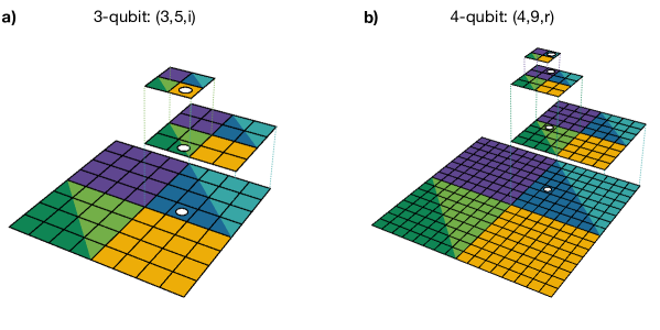
Figure 5: Example determination of the projectors associated to two density matrix elements of 3- and 4-qubit systems using the recursive procedure outlined in the main text. At each state, the density matrix is divided into 4 different quadrants: quadrant “1” is colored in violet, quadrant “2” in blue, quadrant “3” in green, and quadrant “4” in golden yellow. Quadrants “2” and “3” are further subdivided into an upper (lighter) and a lower (darker) part. Each plane represents a successive iteration of the algorithm outlined in the main text, which proceeds from bottom to top. a) The 3-qubit matrix element $\rho_{3,5}^{\mathrm{im}}$ is located in quadrants “$2l3l4$” and corresponds to the $\left|{RDV}\right\rangle$ projector according to Tab. 2 b) 4-qubit matrix element $\rho_{4,9}^{\mathrm{re}}$ is located in quadrants “$2l3u12u$” therefore corresponding to the projector $\left|{RRHD}\right\rangle$ according to Table 2.

To this end, we divide $\pi_{n}$ into four quadrants, with “1” referring to the upper-left quadrant and “4” indicating the lower-right quadrant. Each of the quadrants 2 and 3 is further divided into an upper (“$u$”) and a lower (“$l$”) triangular part. The real part of the elements along the diagonal is assigned to the $u$ portion, while the imaginary part is assigned to the $l$ portion. This subdivision is pictorially represented in Fig. 5.

To determine the projector corresponding to the density-matrix element $\rho_{i,j}$, we initially locate it within $\pi_{n}$ which immediately determines the projector associated with the first qubit, that is $\left|{H}\right\rangle$, $\left|{D}\right\rangle$, $\left|{R}\right\rangle$, or $\left|{V}\right\rangle$ according to its position: 1, $2u$, $2l$, or 4, respectively. We then continue splitting the quadrant where the element is found until we reach a resulting quadrant size of $2\times 2$. At each splitting step, if the element falls into quadrants 1 or 4, the projector associated to the next qubit is $\left|{H}\right\rangle$ (for 1) or $\left|{V}\right\rangle$ (for 4). Conversely, if it falls into quadrants 2 or 3, the projector choice depends on its position in the previous splitting step. For an element in an upper quadrant, we select $\left|{D}\right\rangle$; and, for an element in a lower quadrant, we select $\left|{R}\right\rangle$ unless the previous quadrant was either $2l$ or $3l$, in which case the choice is reversed. Table 2 summarizes these steps.

As an illustration, Fig. 5 shows the determination of two projectors for a 3- and a 4-qubit system. More specifically, in the 3-qubit case, we consider the matrix element $\rho_{3,5}^{\mathrm{im}}$; its successive locations in $\pi_{3}$ are described by the sequence “$2l3l4$” which, according to Table 2, corresponds to the local projector $\left|{RDV}\right\rangle$. The projector associated with $\rho_{4,9}^{\mathrm{re}}$ in a 4-qubit system, is instead determined by the locations in $\pi_{4}$ described by the sequence “$2l3u12u$”; using Table 2, one then finds $\left|{RRHD}\right\rangle$.

Previous quadrant	New quadrant	1-qubit projector
any	1	$\left|{H}\right\rangle$
any	4	$\left|{V}\right\rangle$
any except $2l$, $3l$	$2u$, $3u$	$\left|{D}\right\rangle$
any except $2l$, $3l$	$2l$, $3l$	$\left|{R}\right\rangle$
$2l$, $3l$	$2u$, $3u$	$\left|{R}\right\rangle$
$2l$, $3l$	$2l$, $3l$	$\left|{D}\right\rangle$

Table 2: Table determining the choice of the 1-qubit projector at each recursive step in Eq. (8). In the first step, “previous quadrant” is always “any”. See text and Fig. 5 for details on the procedure.

IV.2 Choice of threshold

The selection of an appropriate threshold value is dependent on the specific physical system used to implement the qubits (e.g., noise level), the amount of available resources (e.g., time requirements), and the desired quantum state to be generated.

In the case of IBMQ quantum processors considered here, it is possible to evaluate an optimal circuit-specific threshold using the IBMQ simulator available in the qiskit package. First, one simulates the unitary evolution of a ground-state initialized quantum register according to the circuit itself (we have used 10,000 shots). Measuring all qubits yields the expected diagonal counts in the absence of errors, which can be separated into zero and non-zero counts. Second, one uses the IBMQ simulator (which includes the effect of noise) to run the circuit a number of times (100 in our case) and record: the maximum value of the counts among the expected zero elements of the diagonal, $c_{0}^{\mathrm{max}}$; and the minimum value of the counts for the smallest expected non-zero diagonal element, $c_{>0}^{\mathrm{min}}$. Third, one defines, in a conservative way: the noise threshold as $t_{0}=c_{0}^{\mathrm{max}}+n\sqrt{c_{0}^{\mathrm{max}}}$; and the signal threshold as $t_{>0}=c_{>0}^{\mathrm{min}}-n\sqrt{c_{>0}^{\mathrm{min}}}$. The square root terms consider the variability of the counts $c_{0}^{\mathrm{max}}$, $c_{>0}^{\mathrm{min}}$ each time the circuit is simulated; the $n$ factor takes finally into account that, for the quantum processors considered, the noise increases with the number of qubits $n$. The optimal threshold is then

$$t=\mathrm{max}(t_{0},t_{>0}).$$ (9)

Obviously, tQST works best whenever $t_{>0}\gg t_{0}$, $t_{>0}\sim t_{0}$ being the worst case having an unfavorable signal-to-noise ratio. In the case of a noiseless system, $t_{0}=0$ and the threshold is determined solely by the smallest non-zero diagonal element of the density matrix.

IV.3 Fidelity lower bound

Fixing a threshold $t$ establishes a lower bound on the fidelity achievable through a tQST reconstruction. Let ${\cal C}_{t}=\{K\mid\sqrt{\rho_{ii}\rho_{jj}}<t\}$, and consider the estimator matrix $\rho_{t}=\{0\quad\forall\ K\in{\cal C}_{t};\sqrt{\rho_{ii}\rho_{jj}}\ {\mathrm{otherwise}}\}$. Then, one has the inequalities Fuchs and Van De Graaf (1999); Haah et al. (2016)

$$1-\sqrt{F(\rho,\rho_{t})}\leq\frac{1}{2}\|\delta_{t}\|_{1},$$ (10a)

$$\|\delta_{t}\|_{1}\leq 2\sqrt{{\mathrm{min}}(r(\rho),r(\rho_{t}))}\|\delta_{t}\|_{2},$$ (10b)

with the fidelity defined according to $F(\rho,\rho_{t})={\mathrm{Tr}}\left[\sqrt{\rho}\rho_{t}\sqrt{\rho}\right]$, $\|{\circ}\|_{1}$ the trace distance, $\delta_{t}=\rho-\rho_{t}$, and $r\left(\rho\right)$ the rank of the density matrix. Now, as $t$ increases, the state purity of $\rho_{t}$ decreases, so that $r(\rho)\leq r(\rho_{t})$; additionally, $\|\delta_{t}\|_{2}\leq\sqrt{\sum_{{\mathcal{C}}_{t}}\rho_{ii}\rho_{jj}}$. Thus, we obtain the lower bound

$$F_{\mathrm{bound}}(t)\geq\left(1-\sqrt{r(\rho)\sum_{{\cal C}_{t}}\rho_{ii}\rho_{jj}}\right)^{2}.$$ (11)

In our investigations, we noticed that the actual tQST fidelity can be significantly greater than the one established by (11).

IV.4 Maximum likelihood reconstruction

After measuring the counts $N_{K}$ associated with the density matrix elements $|\rho_{K}|>t$ using the corresponding projectors, the density matrix is reconstructed by minimizing the function James et al. (2001)

$$L =\sum_{K}\left(\frac{n_{K}-N_{K}}{2\sqrt{n_{K}}}\right)^{2}; n_{K}=\left\langle{P_{K}}\right|\rho\left|{P_{K}}\right\rangle.$$ (12)

In order to minimize $L$, it is necessary to parametrize the density matrix $\rho$, in such a way that it fulfills the physical conditions of being Hermitian and positive definite. A general approach is to write $\rho=T^{\dagger}T$ where $T$ is a triangular matrix. In this case, the number of parameters to be determined grows as $4^{n}$. If one has reasons to believe that $\rho$ describes a high-purity state, then one can express it as $\rho=V^{\dagger}V$ with ${\mathrm{dim}}(V)=r(\rho_{t})\times 2^{n}$. In this case, the parameters needed for the reconstruction will scale more favourably with the system dimension.

IV.5 IBMQ circuits and tomography state experiments

Random circuits were generated through the corresponding qiskit command random_circuit fixing the circuit depth to 3. We performed 10 independent runs for each circuit, with the threshold $t$ fixed as discussed in Sec. IV.2. Due to the presence of noise, different runs may result in different number of measurements, whenever some of the diagonal elements are close to the threshold $t$. Results reported in Sec. II correspond to the run with the minimum number of measurements performed.

For each run, we conducted a qiskit state tomography experiment, wherein the density matrix was reconstructed through a linear inversion of an over-complete set of $6^{n}$ measurements. This process generally yields a non-positive reconstructed state, which is subsequently rescaled to be positively defined. The rescaling is achieved by computing the eigen-decomposition of the state and adjusting its eigenvalues using the method outlined in Ref. Smolin et al. (2012). In Sec. II, we present the reconstruction with the highest fidelity with the circuit’s target state.

Code availability

The code implementing tQST is available upon reasonable request.

Acknowledgments

We thank Prof. Daniel F.V. James of the University of Toronto for useful discussions. This work is supported by PNRR MUR project PE0000023-NQSTI.

Author information

These authors have contributed equally: Daniele Binosi, Giovanni Garberoglio.

Contributions

M.L. conceived the original idea. All authors developed the protocol. D.B. and G.G. developed the code and performed the experiments on IBMQ. All authors have contributed to writing the manuscript. D.B. and G.G. contributed equally to the work.

Corresponding author

Correspondence to Daniele Binosi (binosi@ectstar.eu).

Ethics declaration

Competing interests

All authors declare no competing interests.

References

- Cao et al. (2023) S. Cao, B. Wu, F. Chen, M. Gong, Y. Wu, Y. Ye, C. Zha, H. Qian, C. Ying, S. Guo, et al., Nature 619, 738 (2023).
- Häffner et al. (2005) H. Häffner, W. Hänsel, C. Roos, J. Benhelm, D. Chek-al Kar, M. Chwalla, T. Körber, U. Rapol, M. Riebe, P. Schmidt, et al., Nature 438, 643 (2005).
- Monz et al. (2011) T. Monz, P. Schindler, J. T. Barreiro, M. Chwalla, D. Nigg, W. A. Coish, M. Harlander, W. Hänsel, M. Hennrich, and R. Blatt, Phys. Rev. Lett. 106, 130506 (2011).
- Wang et al. (2016) X.-L. Wang, L.-K. Chen, W. Li, H.-L. Huang, C. Liu, C. Chen, Y.-H. Luo, Z.-E. Su, D. Wu, Z.-D. Li, H. Lu, Y. Hu, X. Jiang, C.-Z. Peng, L. Li, N.-L. Liu, Y.-A. Chen, C.-Y. Lu, and J.-W. Pan, Phys. Rev. Lett. 117, 210502 (2016).
- Zhang et al. (2019) M. Zhang, L.-T. Feng, Z.-Y. Zhou, Y. Chen, H. Wu, M. Li, S.-M. Gao, G.-P. Guo, G.-C. Guo, D.-X. Dai, et al., Light: Science & Applications 8, 41 (2019).
- Gao et al. (2010) W.-B. Gao, C.-Y. Lu, X.-C. Yao, P. Xu, O. Gühne, A. Goebel, Y.-A. Chen, C.-Z. Peng, Z.-B. Chen, and J.-W. Pan, Nature 6, 331 (2010).
- Agnew et al. (2011) M. Agnew, J. Leach, M. McLaren, F. S. Roux, and R. W. Boyd, Phys. Rev. A 84, 062101 (2011).
- Reimer et al. (2019) C. Reimer, S. Sciara, P. Roztocki, M. Islam, L. Romero Cortés, Y. Zhang, B. Fischer, S. Loranger, R. Kashyap, A. Cino, et al., Nature Physics 15, 148 (2019).
- Madsen et al. (2022) L. S. Madsen, F. Laudenbach, M. F. Askarani, F. Rortais, T. Vincent, J. F. Bulmer, F. M. Miatto, L. Neuhaus, L. G. Helt, M. J. Collins, et al., Nature 606, 75 (2022).
- James et al. (2001) D. F. V. James, P. G. Kwiat, W. J. Munro, and A. G. White, Phys. Rev. A 64, 052312 (2001).
- Gross et al. (2010) D. Gross, Y.-K. Liu, S. T. Flammia, S. Becker, and J. Eisert, Phys. Rev. Lett. 105, 150401 (2010).
- Ahn et al. (2019a) D. Ahn, Y. S. Teo, H. Jeong, F. Bouchard, F. Hufnagel, E. Karimi, D. Koutný, J. Řeháček, Z. Hradil, G. Leuchs, and L. L. Sánchez-Soto, Phys. Rev. Lett. 122, 100404 (2019a).
- Ahn et al. (2019b) D. Ahn, Y. S. Teo, H. Jeong, D. Koutný, J. Řeháček, Z. Hradil, G. Leuchs, and L. L. Sánchez-Soto, Phys. Rev. A 100, 012346 (2019b).
- Xin et al. (2017) T. Xin, D. Lu, J. Klassen, N. Yu, Z. Ji, J. Chen, X. Ma, G. Long, B. Zeng, and R. Laflamme, Phys. Rev. Lett. 118, 020401 (2017).
- Derka et al. (1997) R. Derka, V. Buzek, G. Adam, and P. Knight, arXiv preprint quant-ph/9701029 (1997).
- Ferrie (2014) C. Ferrie, Phys. Rev. Lett. 113, 190404 (2014).
- Chapman et al. (2016) R. J. Chapman, C. Ferrie, and A. Peruzzo, Phys. Rev. Lett. 117, 040402 (2016).
- Rambach et al. (2021) M. Rambach, M. Qaryan, M. Kewming, C. Ferrie, A. G. White, and J. Romero, Phys. Rev. Lett. 126, 100402 (2021).
- Aaronson (2018) S. Aaronson, in Proceedings of the 50th annual ACM SIGACT symposium on theory of computing (2018) pp. 325–338.
- Huang et al. (2020) H.-Y. Huang, R. Kueng, and J. Preskill, Nature Physics 16, 1050 (2020).
- Struchalin et al. (2021) G. Struchalin, Y. A. Zagorovskii, E. Kovlakov, S. Straupe, and S. Kulik, PRX Quantum 2, 010307 (2021).
- Zhu et al. (2010) H. Zhu, Y. S. Teo, and B.-G. Englert, Phys. Rev. A 81, 052339 (2010).
- Kaznady and James (2009) M. S. Kaznady and D. F. V. James, Phys. Rev. A 79, 022109 (2009).
- Lukens et al. (2020) J. M. Lukens, K. J. H. Law, A. Jasra, and P. Lougovski, New Journal of Physics 22, 063038 (2020).
- Nielsen and Chuang (2010) M. A. Nielsen and I. L. Chuang, Quantum Computation and Quantum Information (Cambridge University Press, 2010).
- Dür et al. (2000) W. Dür, G. Vidal, and J. I. Cirac, Phys. Rev. A 62, 062314 (2000).
- Riofrio et al. (2017) C. A. Riofrio, D. Gross, S. T. Flammia, T. Monz, D. Nigg, R. Blatt, and J. Eisert, Nature communications 8, 15305 (2017).
- Qiskit contributors (2023) Qiskit contributors, “Qiskit: An open-source framework for quantum computing,” (2023).
- Kanazawa et al. (2023) N. Kanazawa, D. J. Egger, Y. Ben-Haim, H. Zhang, W. E. Shanks, G. Aleksandrowicz, and C. J. Wood, Journal of Open Source Software 8, 5329 (2023).
- Smolin et al. (2012) J. A. Smolin, J. M. Gambetta, and G. Smith, Phys. Rev. Lett. 108, 070502 (2012), arXiv:1106.5458 [quant-ph] .
- Fuchs and Van De Graaf (1999) C. A. Fuchs and J. Van De Graaf, IEEE Transactions on Information Theory 45, 1216 (1999).
- Haah et al. (2016) J. Haah, A. W. Harrow, Z. Ji, X. Wu, and N. Yu, in Proceedings of the forty-eighth annual ACM symposium on Theory of Computing (2016) pp. 913–925.