Characterizing the Average Interstellar Medium Conditions of Galaxies at $z\sim$ 5.6 – 9
with UV and Optical Nebular Lines

Abstract

Ultraviolet (UV; rest-frame $\sim 1200-2000$ Å) spectra provide a wealth of diagnostics to characterize fundamental galaxy properties, such as their chemical enrichment, the nature of their stellar populations, and their amount of Lyman-continuum (LyC) radiation. In this work, we leverage publicly released JWST data to construct the rest-frame UV-to-optical composite spectrum of a sample of 63 galaxies at $5.6<z<9$, spanning the wavelength range from 1500 to 5200 Å. Based on the composite spectrum, we derive an average dust attenuation $E(B-V)_{\mathrm{gas}}=0.16^{+0.10}_{-0.11}$ from H$\beta$/H$\gamma$, electron density $n_{e}=570^{+510}_{-290}$ cm^-3 from the [O II] doublet ratio, electron temperature $T_{e}=17000^{+1500}_{-1500}$ K from the [O III] $\lambda 4363$/[O III] $\lambda 5007$ ratio, and an ionization parameter $\log(U)=-2.18^{+0.03}_{-0.03}$ from the [O III]/[O II] ratio. Using a direct $T_{e}$ method, we calculate an oxygen abundance $12+\log\mathrm{(O/H)}=7.67\pm 0.08$ and the carbon-to-oxygen (C/O) abundance ratio $\log\mathrm{(C/O)}=-0.87^{+0.13}_{-0.10}$. This C/O ratio is smaller than compared to $z=0$ and $z=2$ – 4 star-forming galaxies, albeit with moderate significance. This indicates the reionization-era galaxies might be undergoing a rapid build-up of stellar mass with high specific star-formation rates. A UV diagnostic based on the ratios of C III] $\lambda\lambda 1907,1909$/He II $\lambda 1640$ versus O III] $\lambda 1666$/He II $\lambda 1640$ suggests that the star formation is the dominant source of ionization, similar to the local extreme dwarf galaxies and $z\sim 2$ – 4 He II–detected galaxies. The [O III]/[O II] and C IV/C III] ratios of the composite spectrum are marginally larger than the criteria used to select galaxies as LyC leakers, suggesting that some of the galaxies in our sample are strong contributors to the reionizing radiation.

1 Introduction

One of the most important questions in modern astronomy is how the galaxies in the early Universe evolve and contribute to cosmic reionization. Those galaxies are expected to have an extreme environment capable of producing large amounts of high-energy photons and building up a highly ionized interstellar medium (ISM) that allows the escape of high-energy photons. The highly ionized gas nebulae can also produce a number of emission lines, of which the strengths are determined by the abundance of each species (Maiolino & Mannucci, 2019), the physical condition of gas nebulae (Kewley et al., 2019; Berg et al., 2021; Mingozzi et al., 2022), dust attenuation (Buat et al., 2002), and the nature of ionizing sources (Jaskot & Ravindranath, 2016; Feltre et al., 2016; Xiao et al., 2018; Byler et al., 2020), providing keys to understand the extreme environment in those reionization-era galaxies.

Before the commissioning of the James Webb Space Telescope (JWST; Gardner et al., 2006; Gardner & et al., 2023), early exploration of nebular emission lines in reionization-era galaxies mostly focused on the rest-frame UV lines acquired by ground-based telescopes (e.g., Stark et al., 2015, 2017; Laporte et al., 2017; Hu et al., 2017; Mainali et al., 2017; Hutchison et al., 2019; Topping et al., 2021). The detections of high-ionization UV lines (N V, C IV, He II, C III]) in these works indicate a lower metallicity and a higher ionization field, and hint at the possible activity of central massive black holes or the presence of Population III stars. However, due to the high sky background and strong telluric absorption, only a small number of detections have been achieved and usually only one of the high-ionization lines is detected, leading to large uncertainty on galaxy properties. Indirect constraints from optical emission lines have also been performed based on the mid-infrared multi-band photometry. The observed mid-infrared colors of high-redshift galaxies reveal a significant contribution of [O III] $\lambda\lambda$4959,5007 and H$\beta$ lines (e.g., González et al., 2012; Roberts-Borsani et al., 2016; Smit et al., 2016; Bridge et al., 2019; Endsley et al., 2021), implying a high star formation rate and a highly ionized ISM. However, the broadband photometry cannot resolve into individual lines, limiting a comprehensive analysis of galaxy properties.

The advent of JWST enables the detection of rest-frame UV and optical emission lines of reionization-era galaxies at an unprecedented high signal-to-noise (S/N) ratio and spectral resolution. With the public release of the first JWST data, the rest-frame optical emission lines have been intensively studied with a large sample of galaxies at $z\gtrsim 6$ and have revealed that high-redshift galaxies exhibit generally low oxygen abundance, high ionization, high electron density, and high temperature (e.g., Curti et al., 2023; Rhoads et al., 2023; Tang et al., 2023; Trump et al., 2023; Sanders et al., 2023; Cameron et al., 2023; Williams et al., 2023; Fujimoto et al., 2023; Bunker et al., 2023a; Isobe et al., 2023a; Jung et al., 2023). In contrast, the rest-frame UV lines, providing complementary information on carbon and nitrogen abundance (Feltre et al., 2016; Jones et al., 2023; Isobe et al., 2023b; Arellano-Córdova et al., 2022; Hirschmann et al., 2019, 2023), ionization source classification (Bunker et al., 2023a; Senchyna et al., 2023; Larson et al., 2023), and ionizing photon escaping (Plat et al., 2019), but are considerably weaker compared to the strong optical lines. Nonetheless, we are able to recover the average UV line properties from a high S/N composite spectrum of a large sample of galaxies. In this work, we leverage the publicly released spectroscopic data of reionization-era galaxies from the Cosmic Evolution Early Release Science Survey (CEERS; Finkelstein et al., 2023) and the JWST Advanced Deep Extragalactic Survey (JADES; Eisenstein et al., 2023; Bunker et al., 2023a) to construct the composite spectrum and investigate the rest-frame UV to optical lines.

This paper is organized as follows. We describe the sample in Section 2. In Section 3, we present our method to generate the composite spectrum and measure the line fluxes. In Section 4, we present the measurements of galaxy properties, including dust attenuation, electron density and temperature, and carbon and oxygen abundances. In Section 5, we discuss the evolution of the carbon-to-oxygen (C/O) abundance ratio, the ionization diagnostic, and the ionizing photon leakage.

2 Data and Sample

2.1 NIRSpec Data from CEERS and JADES

The CEERS and JADES NIRSpec observations utilize several combinations of dispersers and filters to achieve low ($R\sim 100$; prism), medium ($R\sim 1000$; G140M/F100LP, G140M/F070LP, G235M/F170LP, G395M/F290LP), and high resolutions ($R\sim 2700$; G395H/F290LP, JADES only) spanning a wavelength coverage of 1 – 5.3 $\mu$m and 0.7 – 5.3 $\mu$m. The goal of this work is to detect and resolve the UV nebular lines by stacking the two-dimensional (2D) NIRSpec spectra. Therefore, we adopt the medium-resolution grating spectra (hereafter M-Grating) from these two surveys.

The CEERS M-Grating data are obtained with the G140M/F100LP, G235M/F170LP, and G395M/F290LP grating/filter pairs, providing a wavelength coverage of 1 – 5.3 $\mu$m. Each configuration has a total exposure time of 3063.667 s. We adopt the NIRSpec data produced by the CEERS collaboration using the STScI JWST Calibration Pipeline (Bushouse et al., 2022). Specifically, we use the JWST pipeline to perform the standard reductions, including the removal of dark current and bias, flat-fielding, background, photometry, wavelength, and slitloss correction for each exposure. We also perform additional reductions to remove the $1/f$ noise and the snowballs. The 2D spectra of each target are then rectified and combined to generate the final 2D spectra. The details of the data reduction are presented in Arrabal Haro et al. (2023) and Arrabal Haro et al. in prep.

The JADES M-Grating data are obtained with the G140M/F070LP, G235M/F170LP, and G395M/F290LP grating/filter pairs, providing a wavelength coverage of 0.7 – 5.3 $\mu$m. The JADES NIRSpec observation is split into three visits and the exposure time for each configuration for each visit is 8,315.667 s. The single object might be observed in multiple visits and thus, the exposure time for individual objects could be 8,315.667, 16,631.334, or 24,947.0 s. The JADES NIRSpec data used in this work is downloaded from the MAST HLSP archive. It is reduced by the JADES collaboration using the NIRSpec GTO collaboration pipeline (Carniani et al. in prep). We refer the readers to Bunker et al. (2023a) for details.

We note that the flux units of the CEERS 2D spectral data products are MJy, while the flux units of JADES data products are erg s^-1 cm^-2 Å^-1. To unify the flux units of data used in this work, we convert the JADES data to the flux units of MJy.

2.2 Redshift Determination

Here we use Marz (Hinton et al., 2016) to estimate the redshifts of CEERS objects. Marz employs a line-matching algorithm (Baldry et al., 2014), which cross-correlates both the emission- and absorption-line features of the template and the observed spectrum. This matches our requirements well as the strong emission lines are usually the only feature of the reionization-era galaxies.

The templates used in Marz include stars, absorption-line galaxies, emission-line galaxies, and quasars. However, since Marz is designed for ground-based optical surveys, the typical rest-frame near-infrared emission lines are not covered in those templates. To enable the redshift determination for both low- and high-redshift galaxies, we use Bagpipes (Carnall et al., 2018) to generate a template with wavelength coverage from 3400 Å to 20000 Å. We adopt a star-formation history including two exponentially-decaying starburst activities with an earlier starburst to form the majority of stellar masses and a late starburst to produce strong emission lines. This template shows significant Balmer series, [O III] $\lambda\lambda 4959,5007$ doublets, Paschen-series, He I $\lambda 10830$, and [S III] $\lambda 9530$ lines. Since the line-matching algorithm is not sensitive to the relative strength between emission lines, altering the Bagpipes input does not significantly change the redshift determination.

To generate the input one-dimensional (1D) spectra, we combine the short- (G140M/F100LP), medium- (G235M/F170LP), and long-wavelength (G395M/F290LP) CEERS 1D spectra by resampling them to a common wavelength grid with the wavelength interval of 6 Å. For the wavelength ranges that are covered by two adjacent grating/filter pairs, we adopt the average of two spectra. In most cases, clear emission lines are detected and an unambiguous redshift can be determined. However, if the 1D spectra are too noisy, we visually inspect the 2D spectra to identify the potential emission lines and then use Marz to estimate redshift with the identified emission lines. If the redshift cannot be estimated, we exclude the object from the final sample.

The redshift estimated by the Marz can sometimes be biased by the noise spikes. Thus, we refine the redshifts of high-redshift galaxies by fitting Gaussian profiles to H$\alpha$, H$\beta$, and/or [O III] $\lambda\lambda 4959,5007$ lines, whichever is applicable, simultaneously with the Marz redshift as a prior and the wavelengths tied based on the vacuum wavelengths. For the JADES objects, we adopt the redshifts measured by the JADES collaboration (Bunker et al., 2023a). Finally, we identified 60 $z>5$ galaxies from the CEERS and 36 $z>5$ galaxies from the JADES with the redshift uncertainties of 30 – 60 km s^-1.

2.3 Sample

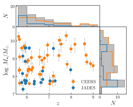
Figure 1: Redshift versus stellar mass diagram of the galaxies used in this work. The orange and blue circles represent the CEERS and JADES samples, respectively. We also present the distributions of the redshift and stellar mass of the sample as the histograms in the top and the bottom right panels. The gray histograms indicate the distributions of the full sample, while the median redshift is 6.33 and the median stellar mass is $10^{8.55}\ M_{\odot}$.

Because we are interested in the rest-frame UV nebular lines, we select the galaxies of which the C IV to C III] are covered by the M-Grating spectra. Further, we constrain the galaxies of which the [O III] $\lambda\lambda 4959,5007$ are also covered as these lines are critical to determining the galaxy properties. These criteria give a redshift range of $5.6<z<9.0$. Additionally, we visually examine the spectra and remove two galaxies that are severely contaminated by artifacts. In total, 42 and 21 galaxies are selected from CEERS and JADES, respectively. We present their properties in Table 4.

In Figure 1, we present the redshift and the stellar mass of the final sample. The stellar mass is estimated by using Bagpipes (Carnall et al., 2018) to fit their multi-wavelength photometry data following the description in Papovich et al. (2023). The redshift is fixed to be the spectroscopic redshift. We used a star-formation history that follows a delayed-$\tau$ model, where SFR $\sim t\times\exp(-t/\tau)$ with $0.1<\tau/\mathrm{Gyr}<10$ and where the age ($t$) is in the range 1 – 2000 Myr. The metallicity is allowed to span 0 – 2.5 $Z_{\odot}$. We allow for dust attenuation following Calzetti et al. (2000) with $A(V)$ in the range 0.0 to 5.0 mag. We include nebular emission with the metallicity of the gas equal to that of the stellar populations, and an ionization parameter, $\log U$ in the range $-4$ to $-1$. We also allow the nebular escape fraction to span from $10^{-4}$ to 1 (following Cole et al. 2023). We use a linear prior on all parameters except the escape fraction, which uses a log-linear prior.

The stellar masses of the final sample cover from $10^{7}$ – $10^{11}$ $M_{\odot}$, while on average the JADES galaxies have lower mass compared to the CEERS galaxies. This is because the CEERS survey is relatively shallower and wider than the JADES survey, and thus preferentially focuses on the brighter galaxies. The median redshift and median stellar mass of the full sample are 6.33 and $10^{8.55}\ M_{\odot}$, respectively.

3 Composite Spectrum and Emission Lines

3.1 Constructing Composite Spectrum

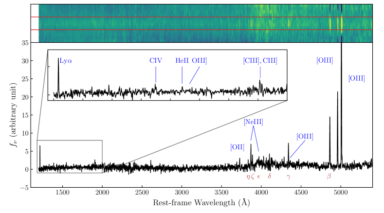
Figure 2: The 2D (top) and 1D (bottom) composite spectra of 63 galaxies at 1200 Å $<\lambda<$ 5400 Å from CEERS and JADES surveys. The 1D composite spectrum is binned by 2 wavelength intervals (i.e., 1 Å) for better illustration. We use blue to label the emission lines detected in this work and use Greek symbols to indicate the hydrogen Balmer lines. The inset panel shows a zoom-in of the wavelength range of 1200 – 2000 Å.

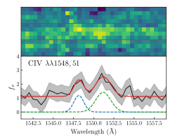
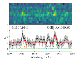
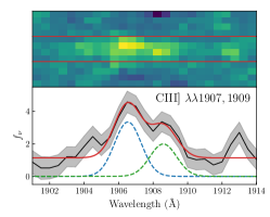
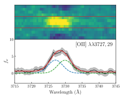
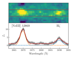
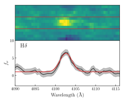
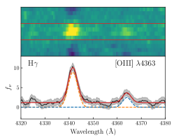
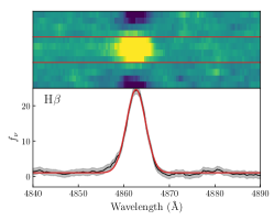
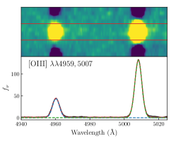
Figure 3: The 2D and unbinned 1D spectra of UV and optical emission lines. In the top panel of each sub-figure, we present the 2D spectra and the extraction window indicated by the two red lines. In the bottom panel of each sub-figure, we present the 1D spectra (black). We use the gray shade to indicate the $1\sigma$ error. The red solid line indicates the best-fit spectra and the orange, blue, or green dashed lines indicate the different components of the best-fit model.

We construct the composite spectrum by median-stacking the normalized 2D spectra of our sample. Compared with the mean-stacking method, the median-stacking method can avoid the spectral features being dominated by the few outliers in the sample. In addition, the 2D-stacking method allows us to inspect the composite 2D spectrum to verify the reliability of emission lines.

For each observed spectrum, we first extract a cutout from the 2D spectrum using a 12-pixel window in the spatial direction (corresponding to 1$\farcs$2) centered on the local maximum of [O III] $\lambda 5007$. In cases where [O III] lacks the spectral coverage, we use H$\alpha$, and if both [O III] and H$\alpha$ are unavailable, we adopt H$\beta$. We then use cubic spline interpolation to shift the spectrum to the rest frame on a common wavelength grid, which covers 1200 – 6000 Å with a wavelength interval of 0.5 Å. An associated variance image is generated based on the error extension and is also shifted to the common wavelength grid. At the same time, we generate a mask image to mask the wavelength range that falls on the NIRSpec detector gaps.

We normalize each spectrum based on the galaxy’s broadband photometry. We adopt the JWST/F150W band to avoid contamination from strong emission lines and Ly$\alpha$ breaks. If JWST/F150W photometry is not available, we adopt the HST/F160W band from CANDELS (Grogin et al., 2011; Koekemoer et al., 2011). Since our objects span a wide redshift range, the JWST/F150W and HST/F160W bands cover different rest-frame wavelengths. To mitigate this effect, we adopt the rest-frame 1500 Å magnitudes as the normalization factors, which are converted from their JWST/F150W or HST/F160W photometry with a UV slope of $f_{\lambda}=\lambda^{-2}$. Our assumption on the UV slope is consistent with the recent observations of reionization-era galaxies (Cullen et al., 2023). In this step, the variance images are also scaled accordingly. We do not attempt to correct the spectra for the dust attenuation here because we cannot reliably measure the Balmer decrement for all the galaxies in the sample (see Section 4.1).

Although the median-stacking method is less prone to outliers, the outliers still potentially bias the composite spectrum and produce artificial signals. By examining the 2D spectra, we find that the outliers usually have very large values compared to other pixels. Thus, we utilize a $10\sigma$-clipping method to effectively remove the extreme outliers, where the $\sigma$ is the median absolute deviation of all pixels used in the stack, and use the median-stacking method to generate the composite 2D spectrum. Meanwhile, the error spectrum is constructed by propagating the variance spectrum of each object.

In the top panel of Figure 2, we present the full 2D composite spectrum derived in this work. The strong emission lines can be easily recognized, along with the faint continuum. Those optical emission lines are extended in spatial direction and are always accompanied by two dark stripes on both sides, which are caused by the nodded background subtraction. The weaker UV emission lines are fainter. Nonetheless, the zoom-in 2D spectra in Figure 3 unambiguously reveal the detections of several UV lines. To compromise between the S/N of UV emission lines, the spatial extent of optical lines, and the dark stripes due to background subtraction, we sum the fluxes within a window of 4 pixels (corresponding to 0.4″) to extract the 1D spectrum. We do not perform additional background subtraction as it has been applied during the raw data reduction. In the bottom panels of Figure 2, we present the full 1D composite spectrum and the zoom-in 1D spectrum of the UV and optical emission lines used in this work.

3.2 Line Measurements

The emission line fluxes are measured by fitting the spectra with Gaussian profiles and a constant continuum $f_{\nu,cont}$. The optical emission lines are sufficiently bright that varying the continuum level does not significantly change the flux measurements. Therefore, the continuum level is a free parameter when fitting the optical lines. However, the UV lines are much weaker and the flux measurements are sensitive to the continuum determination. To mitigate the uncertainty introduced by the continuum determination, we mask the emission lines and adopt the $3\sigma$-clipped median within a wavelength range of $-30$Å to $+30$ Å of emission lines as the continuum levels for UV lines.

We also adopt different recipes for Gaussian components of the UV and optical emission lines:

• C IV $\lambda\lambda 1548,1551$: Since C IV is resonance lines and sometimes show P-Cygni profiles in local galaxies (Mingozzi et al., 2022), the widths and line centers are allowed to vary.

• [C III] $\lambda$1907,C III] $\lambda$1909 (hereafter C III] $\lambda\lambda 1907,1909$): The line centers of C III] $\lambda\lambda 1907,1909$ are fixed to their vacuum wavelengths and the line widths are set to be same.

• He II $\lambda 1640$, O III] $\lambda\lambda 1660,1666$: Since these three emission lines are marginally detected, we fix their line centers based on their vacuum wavelengths. We also set the line widths of O III] $\lambda\lambda 1660,1666$ to be the same and fix the ratio of O III] $\lambda 1666/\lambda 1660$ to be the theoretical value of 2.49 (Aggarwal & Keenan, 1999).

• [O II] $\lambda\lambda 3727,3729$: The [O II] doublet is resolved in our composite spectrum. To separate the two lines, we fix the line centers of [O II] $\lambda\lambda 3727,3729$ lines based on their vacuum wavelengths and set the line widths to be the same.

• [O III] $\lambda\lambda 4959,5007$: We set the widths of [O III] $\lambda\lambda 5007,4959$ to be same, and fix the ratio of [O III] $\lambda 4959/\lambda 5007$ to be the theoretical value of 2.98 (Storey & Zeippen, 2000).

• Balmer lines: Although H$\beta$ and H$\gamma$ lines are detected at very high S/N, allowing us to robustly measure their fluxes, the S/Ns of other Balmer lines are much lower. Thus, to reliably measure the fluxes of fainter Balmer lines, we utilize the information from H$\beta$ line. We first use a Gaussian profile with free width, strength, and line center to fit the H$\beta$ line. We then fix the line widths and centers of the Gaussian profile for other Balmer lines based on H$\beta$.

To estimate the uncertainty of the flux measurements, we adopt a Monte Carlo approach by perturbing the line profiles according to their error spectrum. We generate 1000 realizations for each line and refit them using the above method. Then we adopt the standard deviation of the distribution of flux measurements as the uncertainty. We do not attempt to measure the continuum and the equivalent widths of those lines, because some systematic background issues shown in the 2D composite spectrum (see Figure 2) may result in an overestimation of the continuum and underestimation of the equivalent widths. In Table 1 and Table 2, we list the fluxes of the emission lines of interest.

We do not consider the effect of absorption when we measure the Balmer line fluxes because our composite spectrum cannot resolve them. However, the contribution of Balmer absorption lines, which relies on the average stellar population of our sample, might not be negligible, in particular to the fluxes of high-order Balmer lines. To estimate their contribution, we adopt the relation between the equivalent widths of the Balmer emission line and absorption line presented in Peng et al. (2023). From the composite spectrum, we derive a lower limit of the equivalent width of the H$\gamma$ line to be $>40$ Å. Compared to Figure 4 in Peng et al. (2023), we find that the equivalent width of the H$\gamma$ absorption line should be $\lesssim 3$ Å. Assuming the H$\beta$ and H$\delta$ absorption lines have the same equivalent width as H$\gamma$ absorption line (Groves et al., 2012), we expect the contribution of absorption lines to H$\beta$, H$\gamma$, and H$\delta$ to be $<2.2\%$, $<7.5\%$, and $<15\%$, respectively. We consider these as systematic uncertainties on these emission-line fluxes.

We further acknowledge several potential issues of flux measurement related to the data reduction. First, the flux calibration of the JWST pipeline is based on the pre-launch models, which can result in systematic flux calibration uncertainties in the range of 15% – 40%. Second, the slit losses of the CEERS and JADES data are corrected by assuming the objects are point-like sources and adopting the pre-launch models. In addition, since the PSF of JWST varies significantly with the wavelength (de Graaff et al., 2023), the extraction window adopted in this work can also result in different flux losses for UV and optical emission lines. These three effects are wavelength-dependent and can introduce uncertainties to the absolute flux measurements. Thus, in this work, we focus on the flux ratios of emission lines with small wavelength separations, which are relatively insensitive to these effects.

Table 1: Line Fluxes Relative to H$\beta$ 

Line	Fluxa	Dust-corrected Fluxb
C IV $\lambda$1548	$14.57\pm 7.99$	$33.00\pm 18.08$
C IV $\lambda$1551	$26.20\pm 9.93$	$59.32\pm 22.50$
He II $\lambda$1640	$19.71\pm 6.87$	$42.68\pm 14.87$
O III] $\lambda$1660	$8.28\pm 1.99$	$17.76\pm 4.27$
O III] $\lambda$1666	$20.60\pm 4.97$	$44.00\pm 10.63$
[C III] $\lambda$1907	$34.14\pm 4.98$	$66.16\pm 9.64$
C III] $\lambda$1909	$20.28\pm 4.41$	$39.37\pm 9.67$
[O II] $\lambda$3727	$28.31\pm 3.70$	$34.09\pm 4.45$
[O II] $\lambda$3729	$27.97\pm 3.15$	$33.67\pm 3.79$
[Ne III] $\lambda$3869	$42.07\pm 2.34$	$49.31\pm 2.74$
H$\zeta$	$17.20\pm 2.11$	$20.08\pm 2.46$
H$\delta$	$22.55\pm 1.94$	$25.35\pm 2.18$
H$\gamma$	$43.91\pm 2.20$	$47.45\pm 2.37$
[O III] $\lambda$4363	$11.74\pm 2.05$	$12.64\pm 2.20$
H$\beta$	$100\pm 1.81$	$100\pm 1.81$
[O III] $\lambda$4959	$170.70\pm 0.74$	$168.78\pm 0.73$
[O III] $\lambda$5007	$508.84\pm 2.14$	$498.27\pm 2.10$

Note. — Arbitrary line fluxes measured from the composite spectrum and the dust-corrected composite spectrum.

• The dust-uncorrected line fluxes are presented as the values relative to dust-uncorrected H$\beta$ flux.

• The dust-corrected line fluxes are presented as the values relative to dust-corrected H$\beta$ flux. We adopt a Calzetti et al. (2000) attenuation law with $R_{V}=4.05$ and an $E(B-V)_{\mathrm{gas}}=0.16$ to correct the dust attenuation. For details see Section 4.1.

Table 2: Line Ratios

Line Pair(s)	Flux Ratio
C IV $\lambda\lambda 1548,1551$/He II $\lambda 1640$	$2.16\pm 1.01$
O III] $\lambda 1666$/He II $\lambda 1640$	$1.03\pm 0.44$
C III] $\lambda\lambda 1907,1909$/He II $\lambda 1640$	$2.48\pm 0.92$
C III] $\lambda\lambda 1907,1909$/O III] $\lambda 1666$	$2.40\pm 0.66$
C IV$\lambda\lambda 1548,1551$ /C III] $\lambda\lambda 1907,1909$	$0.874\pm 0.296$
[C III] $\lambda$1907/C III] $\lambda$1909	$1.68\pm 0.41$
[O II] $\lambda$3729/[O II] $\lambda$3727	$1.01\pm 0.18$
[Ne III] $\lambda 3869$/[O II] $\lambda 3727,3729$	$0.727\pm 0.071$
O III] $\lambda$1666/[O III] $\lambda$5007	$0.0883\pm 0.0213$
[O III] $\lambda$4363/[O III] $\lambda$5007	$0.0254\pm 0.0044$
[O III] $\lambda\lambda 4959,5007$/[O II] $\lambda 3727,3729$	$9.84\pm 0.79$
([O III] $\lambda\lambda 4959,5007$+[O II] $\lambda 3727,3729$)/H$\beta$	$7.35\pm 0.15$

Note. — Line ratios calculated based on the dust-corrected line fluxes in Table 1.

4 Results

In this section, we use the line ratios measured in Section 3.2 to derive the average physical properties of the nebular gas in these reionization-era galaxies, including the dust attenuation, the electron density, the electron temperature, and chemical abundance, as shown in Table 3.

4.1 Dust attenuation

Correcting for dust attenuation is necessary when inferring galaxy properties from line ratios, especially lines widely separated in wavelength. The dust attenuation is commonly estimated by comparing the observed Balmer line ratios to the theoretical ratios. To reliably measure the Balmer line ratios, it is required to detect at least two Balmer lines at high S/N ratios. However, most individual galaxy spectra in this work can not provide sufficiently high-S/N Balmer lines for more than a single line ratio. Thus, we do not correct the dust attenuation for individual galaxies. Instead, we adopt the Balmer decrement measured from the composite spectrum to correct the dust attenuation. Here we use the ratios of H$\beta$/H$\gamma$ and H$\beta$/H$\delta$, and assume a Calzetti et al. (2000) attenuation law with $R_{V}=4.05$.

We calculate the intrinsic H$\beta$/H$\gamma$ and H$\beta$/H$\delta$ ratios to be 2.11 and 3.80 using pyneb (Luridiana et al., 2015) assuming a Case B recombination with temperature $T_{e}$ of 17000 K and density $n_{e}$ of 500 cm^-3. The temperature and the density adopted here are consistent with our measurements based on the emission line ratios (see Section 4.2). Comparing the observed ratio to the intrinsic ratio, we obtain the dust attenuation of $E(B-V)_{\mathrm{gas}}=0.16^{+0.10}_{-0.11}$ and $0.21^{+0.12}_{-0.13}$ from H$\beta$/H$\gamma$ and H$\beta$/H$\delta$, which agree within $1\sigma$ uncertainty. We stress again that the contribution of Balmer absorption lines to the emission-line fluxes is not considered here, because they are not resolved in our composite spectrum (see Section 3.2). If we adopt the upper limit of the estimation for Balmer line fluxes estimated in Section 3.2, we obtain the dust attenuation of $E(B-V)_{\mathrm{gas}}=0.06^{+0.10}_{-0.06}$ and $0.04^{+0.10}_{-0.04}$ from H$\beta$/H$\gamma$ and H$\beta$/H$\delta$, respectively. The estimation of dust attenuation from H$\beta$/H$\delta$ is more affected by the underlying absorption. We, therefore, adopt $E(B-V)_{\mathrm{gas}}=0.16$ from H$\beta$/H$\gamma$ and correct the dust attenuation of emission lines using this value. The uncertainty from dust attenuation is roughly $\pm 0.1$ mag, which translates to 10% at 3727 Å and 18% at 1500 Å. The dust-corrected fluxes and line ratios are presented in Table 1 and 2.

4.2 Temperature and Electron Density

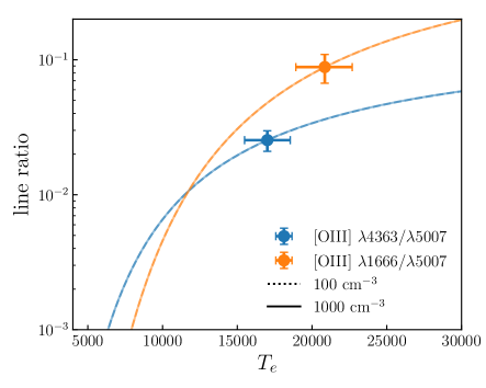
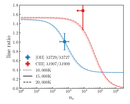
Figure 4: The temperature (left) and electron density (right) diagnostics. We mark the observed line ratios as solid circles. The left panel shows the [O III] $\lambda 4363/\lambda 5007$ (blue) and O III] $\lambda 1666/$[O III] $\lambda 5007$ (orange) ratios as a function of temperature. We present the line ratios for the electron densities of 100 and 1000 cm^-3 as the dotted and solid lines. The relations are nearly unchanged from 100 to 1000 cm^-3. The right panel shows the [O II] $\lambda 3729/\lambda 3727$ (blue) and C III] $\lambda 1907/\lambda 1909$ (red) as a function of electron density. We use dotted, solid, and dashed lines to indicate the line ratios for the temperatures of 10000, 15000, and 20000 K, respectively.

The electron temperature and density are calculated using pyneb and the line ratios observed in this work. For most ions in this work, we adopt the default atomic data in pyneb while assuming a five-level atom model. For O III] $\lambda\lambda 1660,1666$, we adopt the data from Aggarwal & Keenan (1999) which calculates the collision strengths for the necessary six-level atom. For illustration, we use pyneb to calculate the line ratios as a function of temperature and density and present in Figure 4.

We first use O III] $\lambda 1666$/[O III] $\lambda 5007$ and [O III] $\lambda 4363$/[O III] $\lambda 5007$ to calculate the temperature as it is insensitive to the electron density. In the left panel of Figure 4, we present the line ratio-temperature relations for different electron densities and the relations are nearly unchanged from 100 to 1000 cm^-3. We derive temperatures of $17000^{+1500}_{-1500}$ K and $20800^{+1900}_{-1900}$ K from [O III] $\lambda 4363$/[O III] $\lambda 5007$ and O III] $\lambda 1666$/[O III] $\lambda 5007$, respectively. We note a small difference between these two temperatures. This might indicate the UV dust attenuation of high-redshift galaxies deviates from our dust correction constrained by optical Balmer lines. For example, if the UV-dust attenuation is underestimated from the Balmer-line ratios, the intrinsic O III] $\lambda 1666$/[O III] $\lambda 5007$ ratio would increase, bringing it in line with the measurement from [O III] $\lambda 4363$/[O III] $\lambda 5007$. This would require an increase in the O III] $\lambda$1666 flux of about 40%, corresponding to a magnitude correction of $A$(1666 Å) $\approx 0.3-0.4$ mag. On the other hand, as mentioned in Section  3.2, the wavelength-dependent flux losses can result in an overestimation of O III] $\lambda 1666$/[O III] $\lambda 5007$ and thus, overestimate the temperature. Thus, in this work, we adopt the temperature measurement from [O III] $\lambda 4363$/[O III] $\lambda 5007$, which is much less sensitive to these effects. Future studies of JWST spectra of high-redshift galaxies with accurate flux calibration can test the details of the nebular temperature and the UV–optical dust attenuation.

We then use [O II] $\lambda 3729/\lambda 3727$ and C III] $\lambda 1907/\lambda 1909$ lines ratios to calculate the electron densities. As shown in the right panel of Figure 4, the two line ratios probe different electron density ranges: the [O II] $\lambda 3729/\lambda 3727$ is sensitive to 10 – $10^{4}$ cm^-3 while the C III]$\lambda 1907/\lambda 1909$ is sensitive $10^{3}$ – $10^{6}$ cm^-3. These line ratios show little dependence on the temperature, which is relatively small compared to the uncertainties of observed line ratios. Thus, in this work, we assume the [O III] temperature and do not consider the uncertainties introduced by the temperature uncertainty. We obtain electron densities of $570^{+510}_{-290}$ and $<8600$ cm^-3 from [O II] and C III], respectively. The electron density derived from [O II] is consistent with the measurements for individual galaxies at similar redshift (Isobe et al., 2023a). Because the electron density measured from C III] only provides an upper limit, we adopt the measurement from [O II] in this work.

Table 3: Average Galaxy Properties

Property	Line Ratio Used	Value	Note
$z_{\mathrm{med}}$		6.33
$E(B-V)_{\mathrm{gas}}$	H$\beta$/H$\gamma$	$0.16^{+0.10}_{-0.11}$	Section 4.1
	H$\beta$/H$\delta$	$0.21^{+0.12}_{-0.13}$	Section 4.1
$T_{e}(\mathrm{[O\ \textsc{iii}]})$	[O III] $\lambda 4363$/[O III] $\lambda 5007$	$17000^{+1500}_{-1500}$	Section 4.2
	O III] $\lambda 1666$/[O III] $\lambda 5007$	$20800^{+1900}_{-1900}$	Section 4.2
$n_{e}(\mathrm{[O\ \textsc{ii}]})$	[O II] $\lambda 3729/\lambda 3727$	$570^{+510}_{-290}$	Section 4.2
$n_{e}(\mathrm{[C\ \textsc{iii}]})$	C III] $\lambda 1907/\lambda 1909$	$<8600$	Section 4.2
$\log(U)$	[O III] $\lambda\lambda 4959,5007$/[O II] $\lambda\lambda 3727,3729$	$-2.18^{+0.03}_{-0.03}$	Section 4.3.2
$12+\log\mathrm{(O/H)}$	[O III] $\lambda\lambda 4959,5007$/H$\beta$, [O II] $\lambda\lambda 3727,3729$/H$\beta$	$7.672\pm 0.083$	Section 4.3.1
$\log\mathrm{(C/O)}$	C III] $\lambda 1909$/O III] $\lambda 1666$, $\log(U)$	$-0.87^{+0.13}_{-0.10}$	Section 4.3.2
	C III] $\lambda 1909$/O III] $\lambda 1666$, C IV $\lambda\lambda 1548,1551$/C III] $\lambda\lambda 1907,1909$	$-0.70^{+0.13}_{-0.10}$	Section 4.3.2

Note. — Average galaxy properties estimated from the line ratios derived in this work.

4.3 Chemical Abundances

4.3.1 Oxygen abundance

With the temperature and electron density measured above, we are able to use the direct $T_{e}$ method to determine the oxygen abundance, 12 + log(O/H). We adopt the parameterizations for O⁺ and O²⁺ from Peng et al. (2023), which are optimized for the temperature range of 7000 – 25000 K and the density range of 10 – 1000 cm^-3. Because the temperature-sensitive [O II] lines (e.g., [O II] $\lambda\lambda 7320,7330$) are not covered in our composite spectrum, we estimate the [O II] temperature $T_{e}$[O II] from the [O III] temperature $T_{e}$[O III] using the relation in Arellano-Córdova & Rodríguez (2020). We obtain 12 + log(O/H) $=7.672\pm 0.083$ from the composite spectrum, corresponding to 10% of the Solar value (8.69; Asplund et al., 2021).

4.3.2 Carbon-to-Oxygen abundance ratio

We determine the C/O abundance ratio using the C²⁺/O²⁺ ratio and apply a carbon ionization correction factor (ICF) to account for the contribution of C³⁺ ions:

$$\frac{\mathrm{C}}{\mathrm{O}}=\frac{\mathrm{C^{2+}}}{\mathrm{O^{2+}}}\times\left[\frac{X(\mathrm{C^{2+}})}{X(\mathrm{O^{2+}})}\right]^{-1}=\frac{\mathrm{C^{2+}}}{\mathrm{O^{2+}}}\times\mathrm{ICF},$$ (1)

where $X(\mathrm{C^{2+}})$ and $X(\mathrm{O^{2+}})$ are the $\mathrm{C^{2+}}$ and $\mathrm{O^{2+}}$ column fraction, respectively. The C²⁺/O²⁺ abundance is calculated using the C III] $\lambda 1909$/O III] $\lambda 1666$ ratio and the corresponding emissivity ratio calculated by pyneb. We adopt the temperature $T_{e}=17000^{+1500}_{-1500}$ K and electron density $n_{e}=570^{+510}_{-290}$ cm^-3 obtained in Section 4.2 and find log(C²⁺/O²⁺) to be $-0.88^{+0.13}_{-0.10}$, significantly lower than the Solar value, $\log(\mathrm{C/O})=-0.23$ (Asplund et al., 2021). We note that here we assume the C²⁺ zone has the same temperature and electron density as the O²⁺ zone. If we adopt the upper limit of electron density (8600 cm^-3) measured from C III] $\lambda 1907/\lambda 1909$ line flux ratio for the C²⁺ zone, the log(C²⁺/O²⁺) changes by only $\sim 0.005$ dex.

The contribution of C³⁺ ions might not be negligible, as the C IV emission lines are visible in the composite spectrum. We use the photoionization model-derived ICF from Berg et al. (2019) to correct the C³⁺ abundance. Berg et al. (2019) use CLOUDY (Ferland et al., 2013) and BPASS (Eldridge & Stanway, 2016; Stanway et al., 2016) to estimate the ICF as a function of ionization parameter. We use the relations in Berg et al. (2019) for $Z=0.1\ Z_{\odot}$ to convert the [O III]/[O II] (O32) ratio to the ionization parameter and the ICF. We find that the ionization parameter is $\log\ U=-2.18^{+0.03}_{-0.03}$ and the ICF for Equation 1 is $1.026^{+0.008}_{-0.009}$. The errors are propagated from the uncertainty of the [O III]/[O II] ratio and we do not consider the uncertainty from different models, which could be much larger. Applying this modest ICF to C²⁺/O²⁺, we obtain the C/O abundance ratio of log (C/O) $=-0.87^{+0.13}_{-0.10}$.

On the other hand, the detection of C IV allows us to directly estimate the C³⁺/C²⁺ abundance using the C IV/C III] (C43) ratio. Assuming all the observed C IV is from nebular emission and the temperature and density in C³⁺ zone are the same as those in C²⁺, we obtain C³⁺/C²⁺ to be $0.45\pm 0.13$, similar to the C³⁺/C²⁺ recently estimated for one galaxy at $z=6.23$ (Jones et al., 2023). This ratio indicates a correction of $1.45\pm 0.13$ to C²⁺/O²⁺ and leads to a C/O abundance ratio of log (C/O) $=-0.70^{+0.13}_{-0.10}$.

Interestingly, the C43-based ICF is significantly larger than the O32-based ICF, resulting in different estimations of the C/O abundance ratio. This discrepancy is also seen in some low-redshift studies (Berg et al., 2016, 2019). As C IV can also originate from stellar photospheres, this discrepancy might reflect that a large fraction of C IV emission is of stellar origin. For example, by comparing the stellar population model STARBURST99 (Leitherer et al., 1999) to the galaxy spectra at $z\sim 3.1$ – 4.6, Saxena et al. (2022) found that on average $\sim 25\%$ of the C IV flux could be attributed to the stellar origin. Due to insufficient resolution and relatively low S/N in the rest-frame UV, we are unable to directly determine the stellar contribution of C IV. If we assume the excess of C43-based ICF is contributed by the stellar C IV emission, we can find that 91 – 95$\%$ of C IV flux originates from hot stars, rather than the ionized ISM.

In this work, we adopt the C/O abundance ratio derived using the O32-based ICF to avoid the complexity of C IV origins.

5 Discussion

5.1 Interpretation of the C/O Abundance Ratio

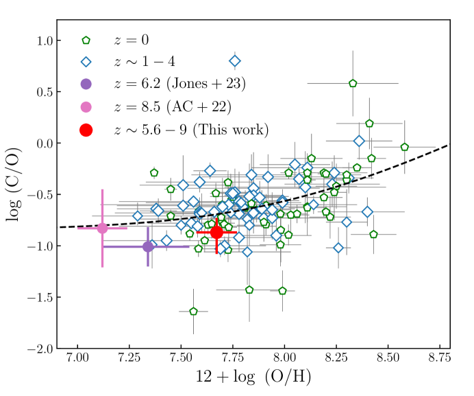
Figure 5: C/O-O/H relationship. We mark our measurement of the composite spectrum as the red circle. For comparison, we compile several objects at $z\sim 0$, $z\sim 1-4$, and $z>6$ from the literature. The first two JWST C/O measurements of reionization-era galaxies are presented as pink (Arellano-Córdova et al., 2022, AC+22 in the figure) and purple (Jones et al., 2023) circles. The green open pentagons mark the measurements of dwarf galaxies at $z\sim 0$ (Berg et al., 2016, 2019; Peña-Guerrero et al., 2017; Senchyna et al., 2017, 2021; Rogers et al., 2023). The blue open diamonds mark the measurements of galaxies at $z\sim 1-4$ (Erb et al., 2010; Christensen et al., 2012; James et al., 2014; Bayliss et al., 2014; Stark et al., 2014; Steidel et al., 2016; Amorín et al., 2017; Berg et al., 2018; Mainali et al., 2020; Matthee et al., 2021; Citro et al., 2023; Iani et al., 2023; Llerena et al., 2023). Motivated by Equation 3 in Nicholls et al. (2017), we use a similar equation to fit the C/O-O/H relation of $z\sim 0$ and $z\sim 1-4$ galaxies, and the best-fit curve is indicated by the black dashed line.

The chemical enrichment of galaxies is a powerful probe for studying galaxy evolution. The relative abundance of carbon to oxygen (C/O) is particularly of interest because those elements are produced by different nucleosynthetic processes on different timescales (for a review see Maiolino & Mannucci, 2019). Oxygen is primarily produced by short-lived massive stars (with lifetimes of $\sim 10$ Myr) and then ejected to the ISM by core-collapse supernovae. The strong outflows driven by short-lived massive stars can also preferentially remove oxygen on short timescales prior to C production. In contrast, carbon enrichment is eventually dominated by the intermediate-mass stars ($2<M/M_{\odot}<8$) during their Asymptotic Giant Branch (AGB) phase (with lifetimes of $\sim 200$ Myr – 1 Gyr). Consequently, the C/O abundance ratio can indicate the key ingredients of galaxy evolution, such as outflows (e.g., Yin et al., 2011) and star formation history (e.g., Berg et al., 2019; Vincenzo & Kobayashi, 2018).

In Figure 5, we compare our C/O-O/H measurements from the composite spectrum of reionization-era galaxies with other measurements from the literature, including the first two JWST C/O measurements of galaxies at $z>6$ (Arellano-Córdova et al., 2022; Jones et al., 2023), measurements of local dwarf galaxies (Berg et al., 2016, 2019; Peña-Guerrero et al., 2017; Senchyna et al., 2017, 2021; Rogers et al., 2023) and intermediate-redshift galaxies ($z\sim 1-4$; Erb et al., 2010; Christensen et al., 2012; James et al., 2014; Bayliss et al., 2014; Stark et al., 2014; Steidel et al., 2016; Amorín et al., 2017; Berg et al., 2018; Mainali et al., 2020; Matthee et al., 2021; Citro et al., 2023; Iani et al., 2023; Llerena et al., 2022, 2023). Although our measurement from the composite spectrum falls within the distribution of $z\sim 0$ and $z\sim 1-4$ galaxies on the C/O-O/H plane, the C/O and O/H ratios of the composite spectrum tend to be lower than the average values at lower redshifts, implying that the reionization-era galaxies on average are more carbon-poor at a given oxygen abundance.

Quantitatively, we follow Nicholls et al. (2017) to fit the distribution of $z\sim 0$ and $z\sim 1-4$ galaxies with a simple expression that combines the two origins of carbon enrichment:

$$\mathrm{log\ (C/O)}=\log\ (10^{a}+10^{[\mathrm{log\ (O/H)+b}]}).$$ (2)

The best-fit curve, denoting the average C/O-O/H relation of low-redshift galaxies, is plotted as the black dashed line in Figure 5. We obtain $a=-0.85$ and $b=-8.88$. Compared to the best-fit curve, the C/O ratio of our composite spectrum is lower by $\sim 1\sigma$.

A potentially smaller C/O ratio with moderate oxygen abundance might suggest that reionization-era galaxies are undergoing a rapid build-up of stellar mass, during which the oxygen has been largely released by supernovae but the secondary carbon enrichment from AGB stars has only mildly proceeded. Considering that secondary carbon enrichment occurs at $>200$ Myr (Maiolino & Mannucci, 2019), this indicates that the majority of the stellar mass is assembled rapidly in these galaxies, on timescales of 100 – 200 Myr ago. This is consistent with the short star-forming episodes ($\lesssim 100$ Myr) inferred from the photometric data of galaxies at these redshifts (e.g., Whitler et al., 2023; Caputi et al., 2023; Cole et al., 2023; Endsley et al., 2023, Papovich, in prep.) This is also in alignment with the chemical abundance calculation of the $z=6.2$ galaxy reported by Jones et al. (2023), for which the C/O abundances suggest a very young age ($<150$ Myr), consistent with its star formation history inferred from modeling its broad-band photometry.

Another possibility is that reionization-era galaxies have a relatively lower preferential removal of oxygen by outflows compared with low-redshift galaxies with similar oxygen abundances. Berg et al. (2019) used a chemical evolution model to demonstrate that the vertical location of the chemical evolutionary track in the C/O-O/H plane is determined by the fraction of oxygen ($X_{\mathrm{out}}$(O)) removed by the outflows. However, this possible origin is at odds with the recent observation of the mass-metallicity relation of reionization-era galaxies. Curti et al. (2023) found that the high-redshift galaxies deviate from the local fundamental metallicity relation, which might hint at the oxygen-enhanced outflows. Consequently, the lower preferential removal of oxygen by outflows is unlikely the case for reionization-era galaxies.

We note again that our measurement significance of a lower C/O ratio in reionization-era galaxies is small and if we adopt the C43-based ICF (i.e., assuming the observed C IV is nebular origin), the C/O ratio of our composite spectrum would agree with the low-redshift trend. Thus, to firmly establish the redshift evolution of C/O ratios, it is necessary to assemble a larger sample of galaxies with measurements of C IV, C III], and O III] at high redshift and discriminate the stellar and nebular contributions to the observed C IV lines.

5.2 Interpretation of the Ionization Properties

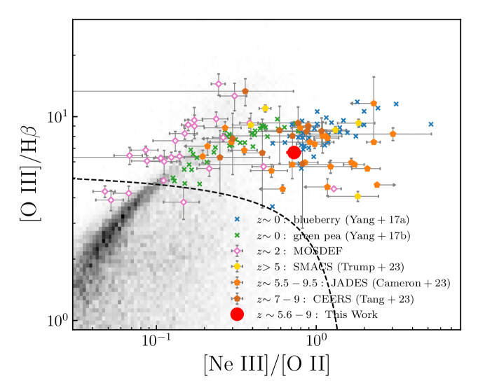
Figure 6: [O III] $\lambda\lambda 4959,5007$/H$\beta$ versus [Ne III] $\lambda 3869$/[O II] $\lambda\lambda 3727,3729$ diagram. The line ratios measured from this work are marked as the red circle. We also plot a series of comparison samples from the literature. The background shows the 2D distribution of $z\sim 0$ galaxies from SDSS (Aihara et al., 2011) and the black dashed line indicates the SF-AGN separator suggested in Backhaus et al. (2022). The local blueberries (Yang et al., 2017a) and green peas (Yang et al., 2017b) are shown as blue and green crosses. The $z\sim 2$ galaxies from the MOSDEF survey (Kriek et al., 2015) are shown as pink diamonds. The recent JWST measurements of galaxies at $z>5$ from SMACS (Trump et al., 2023), JADES (Cameron et al., 2023), and CEERS (Tang et al., 2023) surveys are shown as the yellow, orange, and dark orange pentagons.

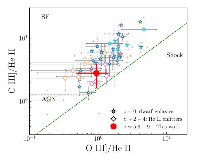
Figure 7: C III] $\lambda\lambda 1907,1909$/He II $\lambda 1640$ versus O III] $\lambda 1666$/He II $\lambda 1640$ diagram. The line ratios measured from this work are marked as the red circle. A series of local galaxies compiled from the literature are marked as purple (Berg et al., 2016), cyan (Berg et al., 2019), green (Senchyna et al., 2017), and blue (Berg et al., 2022; Mingozzi et al., 2023; Olivier et al., 2022) stars. We also include the $z\sim 2-4$ He II emitters as pink (Nanayakkara et al., 2019) and orange (Saxena et al., 2020) diamonds and a $z=6.2$ galaxy as a purple circle (Jones et al., 2023). The lines in this figure that separate star-formation (SF)–AGN and SF–shock regions from Mingozzi et al. (2023) are plotted as the black and green dashed lines, respectively. Compared to the region spanned by the dwarf stars, our measurement is offset to the lower-left region, close to the two well-known dwarf galaxies with the lowest O III]/He II ratios, SBS 0335-052 and I Zw 18.

Recent JWST observations have detected the high ionization lines in several individual galaxies, revealing a diverse nature of ionizing sources in high-redshift galaxies from AGNs, possible Population III stars, to young massive stars (e.g., Fujimoto et al., 2023; Larson et al., 2023; Cleri et al., 2023; Wang et al., 2022; Bunker et al., 2023b). However, it remains unclear which ionizing source is the most common in all high-redshift galaxies. Directly observing the hard ionizing photons from the ionizing source is infeasible. Thus, the flux ratios between emission lines with distinct ionization potentials are frequently used to depict the hardness of the ionizing spectrum. In particular, pairs of lines with small wavelength separations are chosen to mitigate the uncertainties from dust attenuation and observation effects. In this section, we utilize the rest-frame optical and UV line ratio diagnostics to explore the average ionization status in the composite spectrum.

5.2.1 Optical line diagnostics

Figure 6 presents the [O III] $\lambda\lambda 4959,5007$/H$\beta$ versus [Ne III] $\lambda 3869$/[O II] $\lambda\lambda 3727,3729$ diagram (O3Hb-Ne3O2; Trouille et al., 2011; Zeimann et al., 2015) with our measurements shown by the red circle. We also plot a series of comparison samples, including $z\sim 0$ galaxies from the SDSS MPA-JHU catalog (Aihara et al., 2011), $z\sim 0$ dwarf galaxies (including blueberries and green peas from Yang et al., 2017a, b), $z\sim 2$ star-forming galaxies from the MOSDEF survey (Kriek et al., 2015), and reionization-era galaxies from the JWST SMACS, JADES, and CEERS surveys (Trump et al., 2023; Cameron et al., 2023; Tang et al., 2023). Our measurements generally agree with the distributions of individual galaxies in previous JWST studies.

Compared to $z\sim 0$ SDSS galaxies and $z\sim 2$ MOSDEF galaxies, the [Ne III]/[O II] ratio of our composite spectrum is much higher. This is consistent with previous studies of $z\gtrsim 5.5$ galaxies (Cameron et al., 2023; Tang et al., 2023; Trump et al., 2023), indicating that the ionizing sources in the reionization-era galaxies can produce a much harder ionizing spectrum than is typical for $z\sim 0$ – 3 galaxies. However, we are unable to constrain the type of ionizing source from this diagnostic diagram (dashed line in Figure  6), because modes of AGN and star formation can recover the region spanned by the composite spectrum and individual $z>5$ galaxies (see Figure 4 in Cleri et al., 2023). Nonetheless, the local dwarf galaxies (including green peas and blueberries) overlap better with our composite spectrum and the individual galaxies from previous studies. In particular, the blueberries on average have even larger [O III]/H$\beta$ and [Ne III]/[O II] ratios than our composite spectrum. Therefore, the origin of the ionizing source of [Ne III]/[O II] remains uncertain. Studying the local dwarf galaxies could provide clues to understanding the ionizing source in high-redshift galaxies.

5.2.2 UV line diagnostics

Several diagnostic diagrams using UV lines have been proposed in recent works (Feltre et al., 2016; Jaskot & Ravindranath, 2016; Nakajima et al., 2018; Byler et al., 2020; Hirschmann et al., 2022) to distinguish between star-formation, AGN, and shock-driven photoionization. In this work, we adopt the C III] $\lambda\lambda 1907,1909$/He II $\lambda 1640$ versus O III] $\lambda 1666$/He II $\lambda 1640$ diagram (hereafter C3He2-O3He2), which is suggested to show the best classification power among those diagnostics (Mingozzi et al., 2023). In Figure 7, we present our measurements along with those from local dwarf galaxies (Berg et al., 2016, 2019, 2022; Senchyna et al., 2017) and He II emitters at $z\sim 2-4$ (Nanayakkara et al., 2019; Saxena et al., 2020).

We overplot the separators between star formation, AGN, and shocks derived by comparing the ionization models (Gutkin et al., 2016; Feltre et al., 2016; Alarie & Morisset, 2019) with the well-studied local dwarf galaxies (Mingozzi et al., 2023). The position of the composite spectrum in the C3He2-O3He2 diagram indicates that high-redshift galaxies are dominated by ionization from star formation with a modest significance of $\sim 1\sigma$. Hirschmann et al. (2019) also proposed another set of line separators to distinguish between AGN, star formation, and AGN – star-formation composites, obtained by coupling Gutkin et al. (2016) and Feltre et al. (2016) models. However, if we adopt the line separators from Hirschmann et al. (2019, see their Figure 6), our composite spectrum falls in the AGN–star-formation–composite region, suggesting that a large fraction of our sample could host weak AGNs. However, the local dwarf galaxies and He II emitters are also classified as AGN–star-formation composites. Thus, the composite region introduced in Hirschmann et al. (2019) may be more applicable to massive galaxies, where lower-mass galaxies (like local dwarfs and high-redshift galaxies) are more likely to show extreme ionization from star formation instead of having a contribution of weak AGNs.

Compared to the values of C3He2-O3He2 spanned by the local dwarf galaxies, our high-redshift composite spectrum is offset to the lower-left region, close to the two well-known dwarf galaxies with the lowest O III]/He II ratios, SBS 0335-052 and I Zw 18. Our high-redshift composite spectrum overlaps better with the region spanned by the $z\sim 2$ – 4 He II emitters. The offset from the region spanned by most dwarf galaxies might suggest that reionization-era galaxies generally have harder ionizing radiation and are capable of producing more He II ionizing photons ($>54.4$ eV) than those typical dwarf galaxies.

The two extreme dwarf galaxies, SBS 0335-052 and I Zw 18, might be more similar to the high-redshift galaxies and could provide some hints at the He II ionizing sources. In particular, the extended He II $\lambda$4686 emission has already been observed in these two galaxies (Kehrig et al., 2015, 2018; Rickards Vaught et al., 2021). The extended He II $\lambda$4686 emission disfavors the hypothesis that an AGN is the dominant He II ionizing source. X-ray observations would improve the interpretation and rule out other scenarios. For example, ionization from high-mass X-ray binaries is also disfavored by comparing the observed X-ray luminosity to He II luminosity in SBS 0335-052 (Kehrig et al., 2018) and I Zw 18 (Kehrig et al., 2021). Stellar-population models that include the effects of binary stars and their evolution (BPASS; Eldridge et al., 2017; Stanway & Eldridge, 2018) might be able to explain the observed He II fluxes in the SBS 0335-052 (Kehrig et al., 2018), but these models require extremely low metallicities ($Z=0.0005\ Z_{\odot}$). A similar problem is also seen in $z\sim 2$ – 4 He II emitters (Nanayakkara et al., 2019; Saxena et al., 2020) where the He II equivalent widths are usually underpredicted by the BPASS models (Xiao et al., 2018) with more realistic metallicities ($Z=0.005,0.1,1\ Z_{\odot}$). Consequently, additional ionizing sources, such as Wolf-Rayet stars and stripped helium stars (Drout et al., 2023), might still be needed to reproduce the observed line strengths.

On the other hand, the offset could also be (partly) attributed to the lower C/O abundance ratio of reionization-era galaxies (see Section 5.1), which suppresses the carbon emission (Jaskot & Ravindranath, 2016) and decreases the C III]/He II ratio. The overall origin could be a combination of both effects, which is hard to determine yet with our composite spectrum. Distinguishing between these effects would require high-significance detection of UV lines in a large sample of individual galaxies to establish the evolution track of carbon and oxygen enrichment and determine the statistical offset in the UV diagnostic diagrams.

5.3 Ionizing photon leakage

One of the main topics of interest regarding the reionization-era galaxies is to understand how the ionizing photons escape from those galaxies and reionize the Universe. Due to the heavy attenuation of neutral IGM, it is infeasible to directly measure the Lyman continuum (LyC) escape fraction ($f^{\mathrm{esc}}_{\mathrm{LyC}}$) for those galaxies. A variety of indirect probes have been proposed, including the Ly$\alpha$ profile, [O III]/[O II] (O32) ratio, UV absorption lines, Mg II emission line, and C IV emission line (e.g., Izotov et al., 2016; Chisholm et al., 2020; Gazagnes et al., 2020; Hu et al., 2023; Xu et al., 2023; Saxena et al., 2022; Schaerer et al., 2022). We refer the readers to Flury et al. (2022) for a comprehensive discussion of those indirect probes.

The O32 ratio is one of the most frequently used probes to select ionizing-photon leakers as a high O32 ratio might suggest the existence of density-bounded channels through which the ionizing photos can escape. Although the correlation between the $f^{\mathrm{esc}}_{\mathrm{LyC}}$ and O32 ratio is still under debate (Izotov et al., 2018; Katz et al., 2020; Flury et al., 2022), Flury et al. (2022) found a high fraction ($>50\%$) of ionizing-photon leakers in highest-O32 sample (O32 $>10$). Further, Hu et al. (2023) presented an anti-correlation between Ly$\alpha$ peak separation and O32 ratio (see also Jaskot et al., 2019). Although the correlation might be disturbed by the orientation of density-bounded halos, Hu et al. (2023) found that the highest-O32 sample (O32 $>10$) has the smallest Ly$\alpha$ peak separation $<250$ km s^-1, supporting the presence of density-bounded channels. In this work, we obtain an O32 ratio of $9.84\pm 0.79$ from the composite spectrum, close to the criterion suggested by previous works. This would imply that on average the galaxies in our sample have an O32 ratio indicative of non-zero LyC escape.

The resonance line C IV has recently been proposed as a promising probe because the strong C IV line emission is detected in six out of eight ionizing-photon leakers (Schaerer et al., 2022, see also Saxena et al., 2022; Mascia et al., 2023a). This is for several proposed reasons. First, the observation of C IV might suggest the absence of high-column density gas which could scatter the C IV photons. Second, the C IV/C III] (C43) ratio probes the ionization structure, similar to the O32 ratio. In this work, we observe a C43 ratio of $0.874\pm 0.296$, marginally larger than the criterion (C43 $>0.75$) suggested by Schaerer et al. (2022). This again suggests that on average the galaxies in our sample have the conditions for LyC escape observed in other local and moderate-redshift galaxy samples,

Therefore, combining the above evidence, we conclude that indeed there is a moderate fraction of galaxies in our sample that should be the ionizing photon leakers. At the moment our best constraints come from the O32 and C43 line ratios are just at or slightly above the critical values proposed in previous works. This evidence is indirect as we must compare the properties of our galaxies to those from lower redshift studies. Moreover, because we used a stacked spectrum, the exact fraction of galaxies that are leakers, and the fraction of LyC radiation that escapes from them, are unknown. Assuming an extreme case, because we adopt the median stacking, we would expect $\sim 50\%$ of galaxies having O32 $>10$ and $C43>0.75$. Considering that the fraction of ionizing-photon leakers in local galaxies with O32 $>10$ is $\sim 50\%$ (Flury et al., 2022), we would expect that $\sim 25\%$ galaxies in our sample are ionizing-photon leakers. Recently, Mascia et al. (2023b) also studied the ionizing photon escape of CEERS galaxies at $5.6<z<9$ based on an empirical relation between $f^{\mathrm{esc}}_{\mathrm{LyC}}$ and UV slope, H$\beta$ equivalent width, and galaxy size. They found that only $\sim 22\%$ galaxies have $f^{\mathrm{esc}}_{\mathrm{LyC}}>20\%$, consistent with our conclusion. However, much work needs to be done in this area to determine the LyC leakage from individual galaxies in the epoch of reionization.

6 Summary

In this work, we construct a composite spectrum based on the JWST CEERS and JADES NIRSpec M-Grating spectra of 63 galaxies at $5.6<z<9$ with a median redshift of $z_{\mathrm{med}}=6.33$. The composite spectrum covers from rest-frame 1500 Å to 5200 Å, and reliably detects high-ionization UV emission lines, such as C IV, He II, O III], C III], and strong optical emission lines, such as [Ne III], [O II], [O III], H$\beta$. Those emission lines enable us to study the average ISM properties of high-redshift galaxies, such as the chemical abundance, ionization status, and ionizing photon escape. The major results are listed as follows:

• For the nebular gas, we derive an average dust attenuation $E(B-V)_{\mathrm{gas}}=0.16^{+0.10}_{-0.11}$ from H$\beta$/H$\gamma$, an average electron density $n_{e}=570^{+510}_{-290}$ cm^-3 from the [O II] doublet ratio, an electron temperature $T_{e}=17000^{+1500}_{-1500}$ K from the[O III] $\lambda 4363$/[O III] $\lambda 5007$ ratio, and an ionization parameter $\log(U)=-2.18^{+0.03}_{-0.03}$ from the [O III] $\lambda\lambda 4959,5007$/[O II] $\lambda\lambda 3727,3729$ ratio.

• Using a direct method to determine the electron temperature with the ISM conditions and dust attenuation derived in this work, we calculate an oxygen abundance $12+\log\mathrm{(O/H)}=7.672\pm 0.083$ from the O III] $\lambda\lambda 4939,5007$/H$\beta$ and [O II] $\lambda\lambda 3727,3729$/H$\beta$ratios. We also calculate a carbon-to-oxygen (C/O) abundance ratio $\log\mathrm{(C/O)}=-0.87^{+0.13}_{-0.10}$ from the ratio of C III] $\lambda\lambda 1907,1909$/O III] $\lambda 1666$. However, the ICF derived by the C IV $\lambda\lambda 1548,1551$/C III] $\lambda\lambda 1907,1909$ is larger than that derived by the [O III] $\lambda\lambda 4959,5007$/[O II] $\lambda\lambda 3727,3729$. This might suggest that as much as 91 – 95% of the observed C IV emission-line flux originates from stellar photospheres and not the nebular gas.

• Compared to the lower-redshift star-forming galaxies, the composite spectrum of galaxies at $z_{\mathrm{med}}=6.33$ here indicates a smaller C/O ratio at fixed oxygen abundance, albeit with moderate significance. Considering that the oxygen is released by the supernova of massive stars with lifetimes of $\sim 10$ Myr while the carbon can also be released by the longer-lived AGB stars with lifetimes of $>200$ Myr, this result suggests that the stellar mass is assembled quickly, with $\lesssim 100$ Myr, prior to substantial enrichment from the latter.

• We study the optical line-ratio diagnostic diagram of [O III] $\lambda\lambda 4959,5007$/H$\beta$ versus [Ne III] $\lambda 3869$/[O II] $\lambda\lambda 3727,3729$, and the UV line-ratio diagnostic diagram of, C III] $\lambda\lambda 1907,1909$/He II $\lambda 1640$ versus O III] $\lambda 1666$/He II $\lambda 1640$. Our optical diagnostic results are consistent with previous work that high-redshift galaxies have a much harder ionizing spectrum than the $z\sim 0$ – 3 typical galaxies. The UV line-ratio diagnostic diagram also classifies our composite spectrum as high ionization, with a possible presence of weak AGN. The position of the composite spectrum on the UV line-ratio diagnostic diagram overlaps the regions spanned by the local extreme dwarf galaxies, I Zw 18 and SBS 0335-052, and $z\sim 2$ – 4 He II emitters, suggesting high ionization mechanisms. It may be possible to study these lower redshift extreme galaxies as analogs of “normal” star-forming high-redshift galaxies, This can provide clues to the ionization mechanisms in high-redshift galaxies.

• We use the [O III] $\lambda\lambda 4959,5007$/[O II] $\lambda\lambda 3727,3729$ (O32) and C IV $\lambda\lambda 1548,1551$/C III] $\lambda\lambda 1907,1909$ (C43) ratios to infer indirectly an estimate of the average ionizing photon leakage of our sample. These emission-line ratios have been shown to correlate with the LyC radiation escape fraction in low-redshift galaxy studies. The O32 and C43 ratios of the composite spectrum are close to, or marginally larger than, the critical values proposed to indicate LyC radiation leakage. This suggests that at least some of the high-redshift galaxies in our sample should be the ionizing-photon leakers. However, it is unlikely they dominate the galaxy population in our sample given that the values are just at the critical values. Future studies that have direct detections of these line ratios will better constrain the fraction of LyC leakers and the fraction of the LyC radiation that escapes from these galaxies.

Appendix A Object Properties

Table 4 lists the properties of galaxies used in this work.

Table 4: Properties of Galaxies Used in This Work

MSA ID	R.A.	Dec.	$z_{\mathrm{spec}}$	Mag.	log $M_{\star}/M_{\odot}$
CEERS
24	214.897231	52.843854	8.999	28.20a	$8.60^{+0.18}_{-0.28}$
23	214.901253	52.846996	8.880	28.45a	$8.72^{+0.17}_{-0.20}$
1025	214.967532	52.932953	8.714	26.08a	$8.81^{+0.15}_{-0.16}$
1019	215.035392	52.890667	8.678	25.09a	$9.20^{+0.13}_{-0.13}$
1029	215.218762	53.069862	8.610	25.72b	$9.84^{+0.28}_{-0.36}$
1149	215.089714	52.966183	8.175	26.75b	$9.81^{+0.34}_{-0.46}$
4	215.005366	52.996697	7.993	27.72a	$9.55^{+0.22}_{-0.22}$
1027	214.882996	52.840417	7.819	26.40a	$8.69^{+0.19}_{-0.20}$
1023	215.188413	53.033647	7.776	26.23b	$10.30^{+0.21}_{-0.28}$
689	214.999053	52.941977	7.546	25.98b	$9.82^{+0.30}_{-0.42}$
698	215.050317	53.007441	7.471	25.28b	$10.04^{+0.20}_{-0.25}$
1163	214.990468	52.971990	7.448	26.48b	$9.18^{+0.33}_{-0.31}$
1038	215.039717	52.901598	7.194	27.53a	$8.03^{+0.24}_{-0.26}$
499	214.813006	52.834167	7.169	29.24a	$7.71^{+0.27}_{-0.25}$
407	214.839318	52.882566	7.029	28.30a	$7.58^{+0.45}_{-0.38}$
717	215.081406	52.972180	6.932	25.45b	$9.77^{+0.16}_{-0.21}$
1143	215.077006	52.969504	6.927	27.05b	$9.20^{+0.33}_{-0.39}$
1064	215.177167	53.048975	6.790	27.15b	$9.03^{+0.40}_{-0.39}$
613	214.882081	52.844349	6.729	27.33a	$8.51^{+0.27}_{-0.20}$
1414	215.128020	52.984952	6.676	25.90a	$8.92^{+0.21}_{-0.17}$
386	214.832186	52.885082	6.614	28.31a	$8.12^{+0.22}_{-0.27}$
496	214.864737	52.871719	6.569	27.51a	$8.12^{+0.17}_{-0.18}$
1160	214.805047	52.845877	6.568	27.07b	$9.10^{+0.43}_{-0.46}$
1115	215.162817	53.073097	6.300	27.32b	$9.17^{+0.44}_{-0.40}$
792	214.871768	52.833167	6.257	27.67a	$8.50^{+0.26}_{-0.26}$
67	215.015598	53.011857	6.203	28.56a	$8.36^{+0.18}_{-0.21}$
1561	215.166097	53.070755	6.196	27.16b	$9.06^{+0.36}_{-0.36}$
428	214.824554	52.868856	6.102	27.64a	$7.60^{+0.26}_{-0.10}$
355	214.806485	52.878826	6.099	27.04a	$8.42^{+0.20}_{-0.20}$
603	214.867249	52.836736	6.057	26.49a	$8.90^{+0.13}_{-0.17}$
648	214.899825	52.847646	6.053	28.51a	$8.40^{+0.17}_{-0.23}$
618	214.876471	52.839412	6.050	27.13a	$8.32^{+0.14}_{-0.18}$
397	214.836183	52.882678	6.001	25.43a	$8.84^{+0.16}_{-0.13}$
676	214.908480	52.845090	5.990	28.86a	$8.05^{+0.13}_{-0.23}$
1677	215.188738	53.064378	5.867	26.03b	$9.71^{+0.18}_{-0.25}$
403	214.828970	52.875701	5.761	26.18a	$9.60^{+0.10}_{-0.16}$
323	214.872559	52.875948	5.666	27.98a	$7.62^{+0.18}_{-0.15}$
672	214.889680	52.832976	5.666	28.99a	$9.10^{+0.17}_{-0.17}$
515	214.878536	52.874142	5.664	28.26a	$8.37^{+0.17}_{-0.20}$
2168	215.152602	53.057062	5.654	25.23b	$10.09^{+0.17}_{-0.17}$
513	214.819364	52.832533	5.646	28.96a	$8.34^{+0.14}_{-0.16}$
746	214.809145	52.868483	5.623	29.36a	$10.25^{+0.23}_{-0.19}$
JADES
21842	53.156827	$-27.767162$	7.980	28.17c	$8.37^{+0.17}_{-0.21}$
10013682	53.167449	$-27.772034$	7.275	30.30c	$7.75^{+0.21}_{-0.25}$
10013905	53.118327	$-27.769010$	7.197	26.77d	$9.58^{+0.34}_{-0.41}$
20961	53.134230	$-27.768916$	7.045	28.10c	$7.75^{+0.19}_{-0.17}$
4297	53.155794	$-27.815209$	6.714	28.52c	$7.83^{+0.20}_{-0.22}$
3334	53.151381	$-27.819165$	6.706	28.58c	$8.31^{+0.09}_{-0.13}$
16625	53.169047	$-27.778834$	6.631	28.26c	$7.66^{+0.19}_{-0.20}$
18846	53.134918	$-27.772711$	6.335	26.90c	$7.72^{+0.16}_{-0.11}$
18976	53.166602	$-27.772402$	6.327	28.10c	$7.58^{+0.22}_{-0.19}$
17566	53.156101	$-27.775881$	6.102	26.64c	$9.60^{+0.09}_{-0.10}$
19342	53.160623	$-27.771611$	5.974	28.02c	$7.75^{+0.18}_{-0.16}$
10013618	53.119112	$-27.760802$	5.944	26.67d	$9.62^{+0.34}_{-0.29}$
6002	53.110417	$-27.808924$	5.937	27.93c	$7.68^{+0.16}_{-0.15}$
9422	53.121757	$-27.797638$	5.936	27.09c	$7.61^{+0.10}_{-0.09}$
10013704	53.126538	$-27.818090$	5.920	27.83c	$8.85^{+0.14}_{-0.16}$
10013620	53.122590	$-27.760569$	5.917	26.58d	$9.61^{+0.22}_{-0.24}$
19606	53.176568	$-27.771131$	5.889	28.39c	$7.78^{+0.17}_{-0.16}$
10005113	53.167302	$-27.802874$	5.821	28.76c	$7.28^{+0.21}_{-0.14}$
10056849	53.113511	$-27.772836$	5.814	27.64d	$9.15^{+0.33}_{-0.36}$
22251	53.154072	$-27.766072$	5.798	27.63d	$8.16^{+0.14}_{-0.14}$
4404	53.115379	$-27.814774$	5.764	27.40c	$7.66^{+0.14}_{-0.16}$

Note. —

• JWST NIRCam F150W magnitude from the CEERS survey (Finkelstein et al., 2023).

• HST WFC3 F160W magnitude from Finkelstein et al. (2022)

• JWST NIRCam F150W magnitude from the JADES survey data release (Eisenstein et al., 2023).

• HST WFC3 F160W magnitude from Whitaker et al. (2019).

References

- Aggarwal & Keenan (1999) Aggarwal, K. M., & Keenan, F. P. 1999, ApJS, 123, 311, doi: 10.1086/313232
- Aihara et al. (2011) Aihara, H., Allende Prieto, C., An, D., et al. 2011, ApJS, 193, 29, doi: 10.1088/0067-0049/193/2/29
- Alarie & Morisset (2019) Alarie, A., & Morisset, C. 2019, Rev. Mexicana Astron. Astrofis., 55, 377, doi: 10.22201/ia.01851101p.2019.55.02.21
- Amorín et al. (2017) Amorín, R., Fontana, A., Pérez-Montero, E., et al. 2017, Nature Astronomy, 1, 0052, doi: 10.1038/s41550-017-0052
- Arellano-Córdova & Rodríguez (2020) Arellano-Córdova, K. Z., & Rodríguez, M. 2020, MNRAS, 497, 672, doi: 10.1093/mnras/staa1759
- Arellano-Córdova et al. (2022) Arellano-Córdova, K. Z., Berg, D. A., Chisholm, J., et al. 2022, ApJ, 940, L23, doi: 10.3847/2041-8213/ac9ab2
- Arrabal Haro et al. (2023) Arrabal Haro, P., Dickinson, M., Finkelstein, S. L., et al. 2023, ApJ, 951, L22, doi: 10.3847/2041-8213/acdd54
- Asplund et al. (2021) Asplund, M., Amarsi, A. M., & Grevesse, N. 2021, A&A, 653, A141, doi: 10.1051/0004-6361/202140445
- Astropy Collaboration et al. (2013) Astropy Collaboration, Robitaille, T. P., Tollerud, E. J., et al. 2013, A&A, 558, A33, doi: 10.1051/0004-6361/201322068
- Astropy Collaboration et al. (2018) Astropy Collaboration, Price-Whelan, A. M., Sipőcz, B. M., et al. 2018, AJ, 156, 123, doi: 10.3847/1538-3881/aabc4f
- Backhaus et al. (2022) Backhaus, B. E., Trump, J. R., Cleri, N. J., et al. 2022, ApJ, 926, 161, doi: 10.3847/1538-4357/ac3919
- Baldry et al. (2014) Baldry, I. K., Alpaslan, M., Bauer, A. E., et al. 2014, MNRAS, 441, 2440, doi: 10.1093/mnras/stu727
- Bayliss et al. (2014) Bayliss, M. B., Rigby, J. R., Sharon, K., et al. 2014, ApJ, 790, 144, doi: 10.1088/0004-637X/790/2/144
- Berg et al. (2021) Berg, D. A., Chisholm, J., Erb, D. K., et al. 2021, ApJ, 922, 170, doi: 10.3847/1538-4357/ac141b
- Berg et al. (2018) Berg, D. A., Erb, D. K., Auger, M. W., Pettini, M., & Brammer, G. B. 2018, ApJ, 859, 164, doi: 10.3847/1538-4357/aab7fa
- Berg et al. (2019) Berg, D. A., Erb, D. K., Henry, R. B. C., Skillman, E. D., & McQuinn, K. B. W. 2019, ApJ, 874, 93, doi: 10.3847/1538-4357/ab020a
- Berg et al. (2016) Berg, D. A., Skillman, E. D., Henry, R. B. C., Erb, D. K., & Carigi, L. 2016, ApJ, 827, 126, doi: 10.3847/0004-637X/827/2/126
- Berg et al. (2022) Berg, D. A., James, B. L., King, T., et al. 2022, ApJS, 261, 31, doi: 10.3847/1538-4365/ac6c03
- Bridge et al. (2019) Bridge, J. S., Holwerda, B. W., Stefanon, M., et al. 2019, ApJ, 882, 42, doi: 10.3847/1538-4357/ab3213
- Buat et al. (2002) Buat, V., Boselli, A., Gavazzi, G., & Bonfanti, C. 2002, A&A, 383, 801, doi: 10.1051/0004-6361:20011832
- Bunker et al. (2023a) Bunker, A. J., Cameron, A. J., Curtis-Lake, E., et al. 2023a, arXiv e-prints, arXiv:2306.02467, doi: 10.48550/arXiv.2306.02467
- Bunker et al. (2023b) Bunker, A. J., Saxena, A., Cameron, A. J., et al. 2023b, A&A, 677, A88, doi: 10.1051/0004-6361/202346159
- Bushouse et al. (2022) Bushouse, H., Eisenhamer, J., Dencheva, N., et al. 2022, JWST Calibration Pipeline, 1.8.2, Zenodo, Zenodo, doi: 10.5281/zenodo.7325378
- Byler et al. (2020) Byler, N., Kewley, L. J., Rigby, J. R., et al. 2020, ApJ, 893, 1, doi: 10.3847/1538-4357/ab7ea9
- Calzetti et al. (2000) Calzetti, D., Armus, L., Bohlin, R. C., et al. 2000, ApJ, 533, 682, doi: 10.1086/308692
- Cameron et al. (2023) Cameron, A. J., Saxena, A., Bunker, A. J., et al. 2023, A&A, 677, A115, doi: 10.1051/0004-6361/202346107
- Caputi et al. (2023) Caputi, K. I., Rinaldi, P., Iani, E., et al. 2023, arXiv e-prints, arXiv:2311.12691, doi: 10.48550/arXiv.2311.12691
- Carnall et al. (2018) Carnall, A. C., McLure, R. J., Dunlop, J. S., & Davé, R. 2018, MNRAS, 480, 4379, doi: 10.1093/mnras/sty2169
- Chisholm et al. (2020) Chisholm, J., Prochaska, J. X., Schaerer, D., Gazagnes, S., & Henry, A. 2020, MNRAS, 498, 2554, doi: 10.1093/mnras/staa2470
- Christensen et al. (2012) Christensen, L., Laursen, P., Richard, J., et al. 2012, MNRAS, 427, 1973, doi: 10.1111/j.1365-2966.2012.22007.x
- Citro et al. (2023) Citro, A., Berg, D. A., Erb, D. K., et al. 2023, arXiv e-prints, arXiv:2305.14414, doi: 10.48550/arXiv.2305.14414
- Cleri et al. (2023) Cleri, N. J., Olivier, G. M., Hutchison, T. A., et al. 2023, ApJ, 953, 10, doi: 10.3847/1538-4357/acde55
- Cole et al. (2023) Cole, J. W., Papovich, C., Finkelstein, S. L., et al. 2023, arXiv e-prints, arXiv:2312.10152, doi: 10.48550/arXiv.2312.10152
- Cullen et al. (2023) Cullen, F., McLure, R. J., McLeod, D. J., et al. 2023, MNRAS, 520, 14, doi: 10.1093/mnras/stad073
- Curti et al. (2023) Curti, M., Maiolino, R., Curtis-Lake, E., et al. 2023, arXiv e-prints, arXiv:2304.08516, doi: 10.48550/arXiv.2304.08516
- de Graaff et al. (2023) de Graaff, A., Rix, H.-W., Carniani, S., et al. 2023, arXiv e-prints, arXiv:2308.09742, doi: 10.48550/arXiv.2308.09742
- Drout et al. (2023) Drout, M. R., Götberg, Y., Ludwig, B. A., et al. 2023, Science, 382, 1287, doi: 10.1126/science.ade4970
- Eisenstein et al. (2023) Eisenstein, D. J., Johnson, B. D., Robertson, B., et al. 2023, arXiv e-prints, arXiv:2310.12340, doi: 10.48550/arXiv.2310.12340
- Eldridge & Stanway (2016) Eldridge, J. J., & Stanway, E. R. 2016, MNRAS, 462, 3302, doi: 10.1093/mnras/stw1772
- Eldridge et al. (2017) Eldridge, J. J., Stanway, E. R., Xiao, L., et al. 2017, PASA, 34, e058, doi: 10.1017/pasa.2017.51
- Endsley et al. (2021) Endsley, R., Stark, D. P., Chevallard, J., & Charlot, S. 2021, MNRAS, 500, 5229, doi: 10.1093/mnras/staa3370
- Endsley et al. (2023) Endsley, R., Stark, D. P., Whitler, L., et al. 2023, arXiv e-prints, arXiv:2306.05295, doi: 10.48550/arXiv.2306.05295
- Erb et al. (2010) Erb, D. K., Pettini, M., Shapley, A. E., et al. 2010, ApJ, 719, 1168, doi: 10.1088/0004-637X/719/2/1168
- Feltre et al. (2016) Feltre, A., Charlot, S., & Gutkin, J. 2016, MNRAS, 456, 3354, doi: 10.1093/mnras/stv2794
- Ferland et al. (2013) Ferland, G. J., Porter, R. L., van Hoof, P. A. M., et al. 2013, Rev. Mexicana Astron. Astrofis., 49, 137, doi: 10.48550/arXiv.1302.4485
- Finkelstein et al. (2022) Finkelstein, S. L., Bagley, M., Song, M., et al. 2022, ApJ, 928, 52, doi: 10.3847/1538-4357/ac3aed
- Finkelstein et al. (2023) Finkelstein, S. L., Bagley, M. B., Ferguson, H. C., et al. 2023, ApJ, 946, L13, doi: 10.3847/2041-8213/acade4
- Flury et al. (2022) Flury, S. R., Jaskot, A. E., Ferguson, H. C., et al. 2022, ApJ, 930, 126, doi: 10.3847/1538-4357/ac61e4
- Fujimoto et al. (2023) Fujimoto, S., Arrabal Haro, P., Dickinson, M., et al. 2023, ApJ, 949, L25, doi: 10.3847/2041-8213/acd2d9
- Gardner & et al. (2023) Gardner, J. P., & et al. 2023, PASP, 135, 068001, doi: 10.1088/1538-3873/acd1b5
- Gardner et al. (2006) Gardner, J. P., Mather, J. C., Clampin, M., et al. 2006, Space Sci. Rev., 123, 485, doi: 10.1007/s11214-006-8315-7
- Gazagnes et al. (2020) Gazagnes, S., Chisholm, J., Schaerer, D., Verhamme, A., & Izotov, Y. 2020, A&A, 639, A85, doi: 10.1051/0004-6361/202038096
- González et al. (2012) González, V., Bouwens, R. J., Labbé, I., et al. 2012, ApJ, 755, 148, doi: 10.1088/0004-637X/755/2/148
- Grogin et al. (2011) Grogin, N. A., Kocevski, D. D., Faber, S. M., et al. 2011, ApJS, 197, 35, doi: 10.1088/0067-0049/197/2/35
- Groves et al. (2012) Groves, B., Brinchmann, J., & Walcher, C. J. 2012, MNRAS, 419, 1402, doi: 10.1111/j.1365-2966.2011.19796.x
- Gruen et al. (2014) Gruen, D., Seitz, S., & Bernstein, G. M. 2014, PASP, 126, 158, doi: 10.1086/675080
- Gutkin et al. (2016) Gutkin, J., Charlot, S., & Bruzual, G. 2016, MNRAS, 462, 1757, doi: 10.1093/mnras/stw1716
- Hinton et al. (2016) Hinton, S. R., Davis, T. M., Lidman, C., Glazebrook, K., & Lewis, G. F. 2016, Astronomy and Computing, 15, 61, doi: 10.1016/j.ascom.2016.03.001
- Hirschmann et al. (2019) Hirschmann, M., Charlot, S., Feltre, A., et al. 2019, MNRAS, 487, 333, doi: 10.1093/mnras/stz1256
- Hirschmann et al. (2022) —. 2022, arXiv e-prints, arXiv:2212.02522, doi: 10.48550/arXiv.2212.02522
- Hirschmann et al. (2023) —. 2023, MNRAS, 526, 3610, doi: 10.1093/mnras/stad2955
- Hu et al. (2017) Hu, W., Wang, J., Zheng, Z.-Y., et al. 2017, ApJ, 845, L16, doi: 10.3847/2041-8213/aa8401
- Hu et al. (2023) Hu, W., Martin, C. L., Gronke, M., et al. 2023, arXiv e-prints, arXiv:2307.04911, doi: 10.48550/arXiv.2307.04911
- Hutchison et al. (2019) Hutchison, T. A., Papovich, C., Finkelstein, S. L., et al. 2019, ApJ, 879, 70, doi: 10.3847/1538-4357/ab22a2
- Iani et al. (2023) Iani, E., Zanella, A., Vernet, J., et al. 2023, MNRAS, 518, 5018, doi: 10.1093/mnras/stac3198
- Isobe et al. (2023a) Isobe, Y., Ouchi, M., Nakajima, K., et al. 2023a, arXiv e-prints, arXiv:2301.06811, doi: 10.48550/arXiv.2301.06811
- Isobe et al. (2023b) Isobe, Y., Ouchi, M., Tominaga, N., et al. 2023b, arXiv e-prints, arXiv:2307.00710, doi: 10.48550/arXiv.2307.00710
- Izotov et al. (2016) Izotov, Y. I., Schaerer, D., Thuan, T. X., et al. 2016, MNRAS, 461, 3683, doi: 10.1093/mnras/stw1205
- Izotov et al. (2018) Izotov, Y. I., Worseck, G., Schaerer, D., et al. 2018, MNRAS, 478, 4851, doi: 10.1093/mnras/sty1378
- James et al. (2014) James, B. L., Pettini, M., Christensen, L., et al. 2014, MNRAS, 440, 1794, doi: 10.1093/mnras/stu287
- Jaskot et al. (2019) Jaskot, A. E., Dowd, T., Oey, M. S., Scarlata, C., & McKinney, J. 2019, ApJ, 885, 96, doi: 10.3847/1538-4357/ab3d3b
- Jaskot & Ravindranath (2016) Jaskot, A. E., & Ravindranath, S. 2016, ApJ, 833, 136, doi: 10.3847/1538-4357/833/2/136
- Jones et al. (2023) Jones, T., Sanders, R., Chen, Y., et al. 2023, ApJ, 951, L17, doi: 10.3847/2041-8213/acd938
- Jung et al. (2023) Jung, I., Finkelstein, S. L., Arrabal Haro, P., et al. 2023, arXiv e-prints, arXiv:2304.05385, doi: 10.48550/arXiv.2304.05385
- Katz et al. (2020) Katz, H., Ďurovčíková, D., Kimm, T., et al. 2020, MNRAS, 498, 164, doi: 10.1093/mnras/staa2355
- Kehrig et al. (2021) Kehrig, C., Guerrero, M. A., Vílchez, J. M., & Ramos-Larios, G. 2021, ApJ, 908, L54, doi: 10.3847/2041-8213/abe41b
- Kehrig et al. (2018) Kehrig, C., Vílchez, J. M., Guerrero, M. A., et al. 2018, MNRAS, 480, 1081, doi: 10.1093/mnras/sty1920
- Kehrig et al. (2015) Kehrig, C., Vílchez, J. M., Pérez-Montero, E., et al. 2015, ApJ, 801, L28, doi: 10.1088/2041-8205/801/2/L28
- Kewley et al. (2019) Kewley, L. J., Nicholls, D. C., & Sutherland, R. S. 2019, ARA&A, 57, 511, doi: 10.1146/annurev-astro-081817-051832
- Koekemoer et al. (2011) Koekemoer, A. M., Faber, S. M., Ferguson, H. C., et al. 2011, ApJS, 197, 36, doi: 10.1088/0067-0049/197/2/36
- Kriek et al. (2015) Kriek, M., Shapley, A. E., Reddy, N. A., et al. 2015, ApJS, 218, 15, doi: 10.1088/0067-0049/218/2/15
- Laporte et al. (2017) Laporte, N., Nakajima, K., Ellis, R. S., et al. 2017, ApJ, 851, 40, doi: 10.3847/1538-4357/aa96a8
- Larson et al. (2023) Larson, R. L., Finkelstein, S. L., Kocevski, D. D., et al. 2023, ApJ, 953, L29, doi: 10.3847/2041-8213/ace619
- Leitherer et al. (1999) Leitherer, C., Schaerer, D., Goldader, J. D., et al. 1999, ApJS, 123, 3, doi: 10.1086/313233
- Llerena et al. (2022) Llerena, M., Amorín, R., Cullen, F., et al. 2022, A&A, 659, A16, doi: 10.1051/0004-6361/202141651
- Llerena et al. (2023) Llerena, M., Amorín, R., Pentericci, L., et al. 2023, A&A, 676, A53, doi: 10.1051/0004-6361/202346232
- Luridiana et al. (2015) Luridiana, V., Morisset, C., & Shaw, R. A. 2015, A&A, 573, A42, doi: 10.1051/0004-6361/201323152
- Mainali et al. (2017) Mainali, R., Kollmeier, J. A., Stark, D. P., et al. 2017, ApJ, 836, L14, doi: 10.3847/2041-8213/836/1/L14
- Mainali et al. (2020) Mainali, R., Stark, D. P., Tang, M., et al. 2020, MNRAS, 494, 719, doi: 10.1093/mnras/staa751
- Maiolino & Mannucci (2019) Maiolino, R., & Mannucci, F. 2019, A&A Rev., 27, 3, doi: 10.1007/s00159-018-0112-2
- Mascia et al. (2023a) Mascia, S., Pentericci, L., Saxena, A., et al. 2023a, A&A, 674, A221, doi: 10.1051/0004-6361/202245152
- Mascia et al. (2023b) Mascia, S., Pentericci, L., Calabrò, A., et al. 2023b, arXiv e-prints, arXiv:2309.02219, doi: 10.48550/arXiv.2309.02219
- Matthee et al. (2021) Matthee, J., Sobral, D., Hayes, M., et al. 2021, MNRAS, 505, 1382, doi: 10.1093/mnras/stab1304
- Mingozzi et al. (2022) Mingozzi, M., James, B. L., Arellano-Córdova, K. Z., et al. 2022, ApJ, 939, 110, doi: 10.3847/1538-4357/ac952c
- Mingozzi et al. (2023) Mingozzi, M., James, B. L., Berg, D., et al. 2023, arXiv e-prints, arXiv:2306.15062, doi: 10.48550/arXiv.2306.15062
- Nakajima et al. (2018) Nakajima, K., Schaerer, D., Le Fèvre, O., et al. 2018, A&A, 612, A94, doi: 10.1051/0004-6361/201731935
- Nanayakkara et al. (2019) Nanayakkara, T., Brinchmann, J., Boogaard, L., et al. 2019, A&A, 624, A89, doi: 10.1051/0004-6361/201834565
- Nicholls et al. (2017) Nicholls, D. C., Sutherland, R. S., Dopita, M. A., Kewley, L. J., & Groves, B. A. 2017, MNRAS, 466, 4403, doi: 10.1093/mnras/stw3235
- Olivier et al. (2022) Olivier, G. M., Berg, D. A., Chisholm, J., et al. 2022, ApJ, 938, 16, doi: 10.3847/1538-4357/ac8f2c
- Papovich et al. (2023) Papovich, C., Cole, J. W., Yang, G., et al. 2023, ApJ, 949, L18, doi: 10.3847/2041-8213/acc948
- Peña-Guerrero et al. (2017) Peña-Guerrero, M. A., Leitherer, C., de Mink, S., Wofford, A., & Kewley, L. 2017, ApJ, 847, 107, doi: 10.3847/1538-4357/aa88bf
- Peng et al. (2023) Peng, Z., Martin, C. L., Thibodeaux, P., et al. 2023, arXiv e-prints, arXiv:2308.00351, doi: 10.48550/arXiv.2308.00351
- Plat et al. (2019) Plat, A., Charlot, S., Bruzual, G., et al. 2019, MNRAS, 490, 978, doi: 10.1093/mnras/stz2616
- Rhoads et al. (2023) Rhoads, J. E., Wold, I. G. B., Harish, S., et al. 2023, ApJ, 942, L14, doi: 10.3847/2041-8213/acaaaf
- Rickards Vaught et al. (2021) Rickards Vaught, R. J., Sandstrom, K. M., & Hunt, L. K. 2021, ApJ, 911, L17, doi: 10.3847/2041-8213/abf09b
- Roberts-Borsani et al. (2016) Roberts-Borsani, G. W., Bouwens, R. J., Oesch, P. A., et al. 2016, ApJ, 823, 143, doi: 10.3847/0004-637X/823/2/143
- Rogers et al. (2023) Rogers, N. S. J., Scarlata, C. M., Skillman, E. D., et al. 2023, arXiv e-prints, arXiv:2308.10927, doi: 10.48550/arXiv.2308.10927
- Sanders et al. (2023) Sanders, R. L., Shapley, A. E., Topping, M. W., Reddy, N. A., & Brammer, G. B. 2023, arXiv e-prints, arXiv:2301.06696, doi: 10.48550/arXiv.2301.06696
- Saxena et al. (2020) Saxena, A., Pentericci, L., Mirabelli, M., et al. 2020, A&A, 636, A47, doi: 10.1051/0004-6361/201937170
- Saxena et al. (2022) Saxena, A., Cryer, E., Ellis, R. S., et al. 2022, MNRAS, 517, 1098, doi: 10.1093/mnras/stac2742
- Schaerer et al. (2022) Schaerer, D., Izotov, Y. I., Worseck, G., et al. 2022, A&A, 658, L11, doi: 10.1051/0004-6361/202243149
- Senchyna et al. (2023) Senchyna, P., Plat, A., Stark, D. P., & Rudie, G. C. 2023, arXiv e-prints, arXiv:2303.04179, doi: 10.48550/arXiv.2303.04179
- Senchyna et al. (2021) Senchyna, P., Stark, D. P., Charlot, S., et al. 2021, MNRAS, 503, 6112, doi: 10.1093/mnras/stab884
- Senchyna et al. (2017) Senchyna, P., Stark, D. P., Vidal-García, A., et al. 2017, MNRAS, 472, 2608, doi: 10.1093/mnras/stx2059
- Smit et al. (2016) Smit, R., Bouwens, R. J., Labbé, I., et al. 2016, ApJ, 833, 254, doi: 10.3847/1538-4357/833/2/254
- Stanway & Eldridge (2018) Stanway, E. R., & Eldridge, J. J. 2018, MNRAS, 479, 75, doi: 10.1093/mnras/sty1353
- Stanway et al. (2016) Stanway, E. R., Eldridge, J. J., & Becker, G. D. 2016, MNRAS, 456, 485, doi: 10.1093/mnras/stv2661
- Stark et al. (2014) Stark, D. P., Richard, J., Siana, B., et al. 2014, MNRAS, 445, 3200, doi: 10.1093/mnras/stu1618
- Stark et al. (2015) Stark, D. P., Walth, G., Charlot, S., et al. 2015, MNRAS, 454, 1393, doi: 10.1093/mnras/stv1907
- Stark et al. (2017) Stark, D. P., Ellis, R. S., Charlot, S., et al. 2017, MNRAS, 464, 469, doi: 10.1093/mnras/stw2233
- Steidel et al. (2016) Steidel, C. C., Strom, A. L., Pettini, M., et al. 2016, ApJ, 826, 159, doi: 10.3847/0004-637X/826/2/159
- Storey & Zeippen (2000) Storey, P. J., & Zeippen, C. J. 2000, MNRAS, 312, 813, doi: 10.1046/j.1365-8711.2000.03184.x
- Tang et al. (2023) Tang, M., Stark, D. P., Chen, Z., et al. 2023, MNRAS, doi: 10.1093/mnras/stad2763
- Topping et al. (2021) Topping, M. W., Shapley, A. E., Stark, D. P., et al. 2021, ApJ, 917, L36, doi: 10.3847/2041-8213/ac1a79
- Trouille et al. (2011) Trouille, L., Barger, A. J., & Tremonti, C. 2011, ApJ, 742, 46, doi: 10.1088/0004-637X/742/1/46
- Trump et al. (2023) Trump, J. R., Arrabal Haro, P., Simons, R. C., et al. 2023, ApJ, 945, 35, doi: 10.3847/1538-4357/acba8a
- Vincenzo & Kobayashi (2018) Vincenzo, F., & Kobayashi, C. 2018, A&A, 610, L16, doi: 10.1051/0004-6361/201732395
- Wang et al. (2022) Wang, X., Cheng, C., Ge, J., et al. 2022, arXiv e-prints, arXiv:2212.04476, doi: 10.48550/arXiv.2212.04476
- Whitaker et al. (2019) Whitaker, K. E., Ashas, M., Illingworth, G., et al. 2019, ApJS, 244, 16, doi: 10.3847/1538-4365/ab3853
- Whitler et al. (2023) Whitler, L., Endsley, R., Stark, D. P., et al. 2023, MNRAS, 519, 157, doi: 10.1093/mnras/stac3535
- Williams et al. (2023) Williams, H., Kelly, P. L., Chen, W., et al. 2023, Science, 380, 416, doi: 10.1126/science.adf5307
- Xiao et al. (2018) Xiao, L., Stanway, E. R., & Eldridge, J. J. 2018, MNRAS, 477, 904, doi: 10.1093/mnras/sty646
- Xu et al. (2023) Xu, X., Henry, A., Heckman, T., et al. 2023, ApJ, 943, 94, doi: 10.3847/1538-4357/aca89a
- Yang et al. (2017a) Yang, H., Malhotra, S., Rhoads, J. E., & Wang, J. 2017a, ApJ, 847, 38, doi: 10.3847/1538-4357/aa8809
- Yang et al. (2017b) Yang, H., Malhotra, S., Gronke, M., et al. 2017b, ApJ, 844, 171, doi: 10.3847/1538-4357/aa7d4d
- Yin et al. (2011) Yin, J., Matteucci, F., & Vladilo, G. 2011, A&A, 531, A136, doi: 10.1051/0004-6361/201015022
- Yung et al. (2020) Yung, L. Y. A., Somerville, R. S., Finkelstein, S. L., et al. 2020, MNRAS, 496, 4574, doi: 10.1093/mnras/staa1800
- Zeimann et al. (2015) Zeimann, G. R., Ciardullo, R., Gebhardt, H., et al. 2015, ApJ, 798, 29, doi: 10.1088/0004-637X/798/1/29