Exploring magnetic fluctuations effects in QED gauge fields: implications for mass generation

Abstract

In this work, we calculate the one-loop contribution to the polarization tensor for photons (and gluons) in the presence of a classical background magnetic field with white-noise stochastic fluctuations. The magnetic field fluctuations are incorporated into the fermion propagator in a quasi-particle picture, which we developed in previous works using the replica trick. By focusing on the strong-field limit, here we explicitly calculate the polarization tensor. Our results reveal that it does not satisfy the transversality conditions outlined by the Ward identity, thus breaking the $U(1)$ symmetry. As a consequence, in the limit of vanishing photon four-momenta, the tensor coefficients indicate the emergence of an effective magnetic mass induced on photons (and gluons) by these stochastic fluctuations, leading to the interpretation of a dispersive medium with a noise-dependent index of refraction.

I Introduction

Understanding the properties of photons and gluons in thermal and magnetized media is essential for a proper interpretation of the observables arising from current high-energy experiments David (2020); Adare et al. (2015). Recent studies on photon production in heavy-ion collisions (HIC) have revealed that photons originating from such scenarios exhibit an elliptic flow coefficient, denoted as $v_{2}$, of similar magnitude to that measured in hadrons Adare et al. (2012); Acharya et al. (2019); Adare et al. (2016). Various sources of photons have been proposed to characterize the observed spectrum. A significant photon yield is generated during the equilibrium stages of HIC, which is utilized to estimate the temperature of the colliding system Ghiglieri (2014). On the other hand, direct photons are believed to be produced during the hadronization stages of HIC, where much of the $v_{2}$ is generated. Furthermore, prompt photons are identified as part of the low $p_{\text{T}}$ spectra Paquet et al. (2016a). Despite the aforementioned identified sources of photons, there remains a discrepancy between the theoretical models developed to describe the photon spectra and the corresponding experimental measurements. In particular, an excess of low-$p_{\text{T}}$ photons is obtained when comparing theory and experimental data Paquet et al. (2016b).

In an effort to provide a more comprehensive description of the experimental data, recent studies have suggested that the production of prompt photons may be influenced by the intense magnetic fields generated during the initial stages of the collision Ayala et al. (2022, 2020a, 2017); Jia et al. (2023). These investigations propose that the background magnetic field induces gluon fusion and splitting processes for photon generation due to the high-density gluon occupation, referred to as the Color Glass Condensate (CGC) Lappi and McLerran (2006); McLerran and Schenke (2014); Harland-Lang et al. (2015); Carrington et al. (2022). Although this hypothesis leads to an improved description of the elliptic flow and yield, the kinematic restrictions arising from the vanishing mass of photons and gluons reduce the available phase space for the number of photons Adler et al. (1970). Therefore, any modification in the dispersion relations for gluons and photons induced by the medium may open up a richer physical scenario. For instance, it is well-known that a thermalized medium can induce an effective photon/gluon mass Nieves et al. (1983); Le Bellac (1996). Similar effects may in principle arise from a magnetized medium, described by a noisy background magnetic field, and this is the main focus of the present work.

Very intense magnetic fields are generated in semi-central HIC by the presence of spectator particles, but they rapidly decay Voronyuk et al. (2011); Adam et al. (2021). This leads to an incomplete electromagnetic response in the effective medium formed at later times, such as the Quark-Gluon Plasma (QGP) Wang et al. (2022). Consequently, the magnetic field is found to be particularly intense during the pre-equilibrium stage. Nevertheless, from a theoretical perspective, the screening effects from magnetized media do not modify the dispersion relation when a constant magnetic field is taken into account Ayala et al. (2021).

The absence of an induced photon/gluon mass in a uniformly magnetized medium arises from symmetry considerations. In the context of the one-loop polarization tensor approximation, the $U(1)$ symmetry remains intact in a constant background magnetic field, as the Ward-Takahashi identity is still satisfied under such condition Ayala et al. (2020b). As a consequence, the inverse propagator for gauge fields continues to exhibit a pole at $q^{2}=0$, thus implying the absence of an induced magnetic mass. Therefore, a physical condition that breaks such a symmetry may lead to the generation of a magnetic gluon/photon mass.

In two of our recent works Castaño Yepes et al. (2023a, b), we investigated the implications of classical background magnetic field, possessing stochastic fluctuations, on the properties of a QED medium. We model this scenario by assuming that the classical background magnetic field arises from a classical gauge field $A_{\text{BG}}^{i}(x)+\delta A_{\text{BG}}^{i}(x)$ with white-noise correlated stochastic fluctuations $\delta A_{\text{BG}}^{i}(x)$, as described by the statistical properties Castaño Yepes et al. (2023a, b)

$$\langle\delta A_{\text{BG}}^{i}(x)\rangle = 0$$

$$\langle\delta A_{\text{BG}}^{i}(x)\delta A_{\text{BG}}^{j}(y)\rangle = \Delta_{B}\delta_{ij}\delta(x-y).$$ (1)

By applying the so-called replica trick Mézard and Parisi (1991), we derived an effective interaction term for QED fermions in the presence of such a noisy magnetic field. This approximation leads, at the perturbative level, to a renormalization of the fermion propagator that now represents quasiparticles propagating in a dispersive medium Castaño Yepes et al. (2023a). On the other hand, when we apply our analysis at the mean field level, the emergence of vector currents is predicted Castaño Yepes et al. (2023b). Both perspectives point towards violations of $U(1)$ symmetry due to the presence of stochastic fluctuations in the background magnetic field.

In this work, we apply our results obtained in Ref. Castaño Yepes et al. (2023a) to calculate the one-loop polarization tensor for photons and gluons, and we find that it is explicitly non-transverse in the sense of the Ward-Takahashi identity. This effect arises from to the breaking of $U(1)$ symmetry due to the incoherent, stochastic nature of the classical background gauge field $A_{\text{BG}}^{\mu}(x)+\delta A_{\text{BG}}^{\mu}(x)$, thus resulting in the generation of a dynamical magnetic mass for the quantum gauge fields (photons and gluons).

II The photon polarization tensor at strong magnetic field

Our starting point is the one-loop contribution to the photon/gluon polarization tensor, which is depicted in Fig. 1 and is given by

$$\mathrm{i}\Pi_{\Delta}^{\mu\nu} = -\frac{1}{2}\int\frac{d^{4}k}{(2\pi)^{4}}\text{Tr}\Big{\{}\mathrm{i}q_{f}\gamma^{\nu}\mathrm{i}S_{\Delta}^{(-)}\left(k\right)\mathrm{i}q_{f}\gamma^{\mu}\mathrm{i}S_{\Delta}^{(-)}(k-p)\Big{\}}$$

$$- \frac{1}{2}\int\frac{d^{4}k}{(2\pi)^{4}}\text{Tr}\Big{\{}\mathrm{i}q_{f}\gamma^{\nu}\mathrm{i}S_{\Delta}^{(+)}(-k+p)\mathrm{i}q_{f}\gamma^{\mu}\mathrm{i}S_{\Delta}^{(+)}(-k)\Big{\}},$$

where $q_{f}$ is the electric charge of the fermion in the loop, and the antiparticle or charge conjugated contribution has been taken into account.

Figure 1: Feynmann diagrams that contribute to the one-loop photon polarization tensor. The arrows in the propagators represent the direction of the flow of charge, whereas the dashed arrows represent the momentum flux.

Note that the only difference between the photon and gluon polarization tensors arises from the trace over color $SU(3)$ space, i.e.,

$$\mathrm{i}\Pi_{\text{gluon}}^{\mu\nu}=\text{Tr}\left\{{t_{a}t_{b}}\right\}\mathrm{i}\Pi_{\text{photon}}^{\mu\nu}=\frac{1}{2}\delta_{ab}\,\mathrm{i}\Pi_{\text{photon}}^{\mu\nu},$$ (3)

where $t_{a,b}$ are the generators of the color group in the fundamental representation.

To analytically compute Eq. (II), we will employ the renormalized fermion propagator in the presence of static (quenched) white noise spatial fluctuations, focusing on the regime of a strong external magnetic field Castaño Yepes et al. (2023a, b). Specifically, the effective fermion-fermion interaction arises as a result of averaging over the background magnetic noise, where we include the magnetic noise-induced interaction effects by dressing the Schwinger propagator with a self-energy, as shown diagrammatically in the Dyson equation depicted in Fig. 2. We remark that for this theory, the skeleton diagram for the self-energy is represented in Fig. 3, and the dressed propagator is provided by

Figure 2: Dyson equation for the ”dressed” propagator (double-line), in terms of the free propagator (single-line) and the self-energy $\Sigma$.

Figure 3: Skeleton diagram representing the self-energy for the effective interacting theory. The dashed line is the disorder-induced interaction $\Delta_{B}$, while the box $\hat{\Gamma}$ represents the 4-point vertex function.

Figure 4: Self-energy diagram at first order in $\Delta=q_{f}^{2}\Delta_{B}$.

$$\mathrm{i}S_{\Delta}^{(\pm)}(p) = C(p)\left(m+\gamma_{0}p^{0}+\frac{\gamma_{3}p^{3}}{z(p)}\right)\mathcal{P}^{(\pm)}(p),$$

where $m$ is the fermion mass and

$$C(p) = \mathrm{i}\frac{z(p)\,e^{-\mathbf{p}_{\perp}^{2}/|q_{f}B|}}{p_{\parallel}^{2}-z^{2}(p)m^{2}},$$ (5a)

$$z(p)=1+\frac{3}{4}\frac{\Delta|q_{f}B|e^{-\mathbf{p}_{\perp}^{2}/|q_{f}B|}}{\pi\sqrt{p_{0}^{2}-m^{2}}}.$$ (5b)

$$z_{3}(p)=\frac{1}{z(p)}\left(1+\frac{\Delta|q_{f}B|e^{-\mathbf{p}_{\perp}^{2}/|q_{f}B|}}{4\pi\sqrt{p_{0}^{2}-m^{2}}}\right),$$ (5c)

$$\mathcal{P}^{(\pm)}(p)=\frac{1}{2}\left[1\pm{\rm sign}(q_{f}B)\mathrm{i}z_{3}(p)\gamma^{1}\gamma^{2}\right].$$ (5d)

As explained in Ref. Castaño Yepes et al. (2023a), the fermion propagator self-energy was computed to order $\Delta\equiv q_{f}^{2}\Delta_{B}$. Therefore, to maintain consistency with this level of approximation, we expand Eq. (LABEL:eq:Prop_Delta) as follows:

$$\mathrm{i}S_{\Delta}^{(\pm)}(p) = \mathrm{i}S_{0}^{(\pm)}(p)+\mathrm{i}\Delta\left(\frac{|q_{f}B|}{2\pi}\right)\Big{[}\Theta_{1}(p)(\not{p}_{\parallel}+m)\mathcal{O}^{(\pm)}$$ (6)

$$- \Theta_{2}(p)\gamma^{3}\mathcal{O}^{(\pm)}\pm\Theta_{3}(p)\mathrm{i}\gamma^{1}\gamma^{2}(\not{p}_{\parallel}+m)\Big{]}$$

$$+ \text{O}(\Delta^{2}),$$

where

$$\mathrm{i}S_{0}^{(\pm)}(p) = 2\mathrm{i}\frac{e^{-\mathbf{p}_{\perp}^{2}/|q_{f}B|}}{p_{\parallel}^{2}-m^{2}}(\not{p}_{\parallel}+m)\mathcal{O}^{(\pm)}$$ (7)

is the fermion propagator in the presence of an intense magnetic field, the spin-projection operator is given by

$$\mathcal{O}^{(\pm)} = \frac{1}{2}\left[1\pm{\rm sign}(q_{f}B)\mathrm{i}\gamma^{1}\gamma^{2}\right],$$ (8)

and we defined the functions

$$\Theta_{1}(p) \equiv \frac{3(p_{\parallel}^{2}+m^{2})e^{-2\mathbf{p}_{\perp}^{2}/|q_{f}B|}}{(p_{\parallel}^{2}-m^{2})^{2}\sqrt{p_{0}^{2}-m^{2}}},$$ (9a)

$$\Theta_{2}(p) \equiv \frac{3p_{3}e^{-2\mathbf{p}_{\perp}^{2}/|q_{f}B|}}{(p_{\parallel}^{2}-m^{2})\sqrt{p_{0}^{2}-m^{2}}},$$ (9b)

$$\Theta_{3}(p) \equiv \frac{e^{-2\mathbf{p}_{\perp}^{2}/|q_{f}B|}}{(p_{\parallel}^{2}-m^{2})\sqrt{p_{0}^{2}-m^{2}}}.$$ (9c)

Here, we separated the parallel ($\parallel$) from the perpendicular ($\perp$) Minkowski subspaces, as defined by their relative direction with respect to the background external magnetic field, by splitting the metric tensor as

$$g^{\mu\nu}=g_{\parallel}^{\mu\nu}+g_{\perp}^{\mu\nu},$$ (10a)

where

$$g_{\parallel}^{\mu\nu} = \text{diag}(1,0,0,-1)$$

$$g_{\perp}^{\mu\nu} = \text{diag}(0,-1,-1,0).$$ (10b)

The latter implies that for any four-vector

$$p^{\mu} = p_{\parallel}^{\mu}+p_{\perp}^{\mu},$$ (11a)

we get

$$p^{2}=p_{\parallel}^{2}-\mathbf{p}_{\perp}^{2},$$ (11b)

with

$$p_{\parallel}^{2} = p_{0}^{2}-p_{3}^{2}$$

$$\mathbf{p}_{\perp}^{2} = p_{1}^{2}+p_{2}^{2}.$$ (11c)

Hence, Eq. (II) takes the form:

$$\mathrm{i}\Pi_{\Delta}^{\mu\nu} = \mathrm{i}\Pi_{0}^{\mu\nu}+\mathrm{i}\frac{q_{f}^{2}|q_{f}B|\Delta}{4\pi}\sum_{i=1}^{3}T_{i}^{\mu\nu},$$ (12)

where $\mathrm{i}\Pi_{0}^{\mu\nu}$ is the one-loop polarization tensor in the strong field limit and in the absence of fluctuations Fukushima (2011):

$$\mathrm{i}\Pi_{0}^{\mu\nu}=\frac{\mathrm{i}q_{f}^{2}|q_{f}B|}{4\pi^{2}}e^{-\mathbf{p}_{\perp}^{2}/2|q_{f}B|}p_{\parallel}^{2}\mathcal{I}_{0}(p_{\parallel}^{2})\left(g_{\parallel}^{\mu\nu}-\frac{p_{\parallel}^{\mu}p_{\parallel}^{\nu}}{p_{\parallel}^{2}}\right)$$ (13)

so that (see Appendix A)

$$\mathcal{I}_{0}(p_{\parallel}^{2}) = \int_{0}^{1}dx\frac{x(1-x)}{x(1-x)p_{\parallel}^{2}-m^{2}}$$

$$= \frac{1}{p_{\parallel}^{2}}\left[1+\frac{2m^{2}/p_{\parallel}^{2}}{\sqrt{1-\frac{4m^{2}}{p_{\parallel}^{2}}}}\log\left[\frac{1+\sqrt{1-\frac{4m^{2}}{p_{\parallel}^{2}}}}{1-\sqrt{1-\frac{4m^{2}}{p_{\parallel}^{2}}}}\right]\right],$$

and the tensors $T_{i}^{\mu\nu}$ are given by:

$$T_{1}^{\mu\nu} \equiv 16\mathrm{i}\int\frac{d^{4}k}{(2\pi)^{4}}\frac{e^{-\mathbf{k}_{\perp}^{2}/|q_{f}B|}}{k_{\parallel}^{2}-m^{2}}\Theta_{1}(k-p)\Bigg{[}(m^{2}+k_{\parallel}\cdot(p_{\parallel}-k_{\parallel}))(g_{\parallel}^{\mu\nu}-g_{\perp}^{\mu\nu})+(k_{\parallel}^{\mu}-p_{\parallel}^{\mu})k_{\parallel}^{\nu}+k_{\parallel}^{\mu}(k_{\parallel}^{\nu}-p_{\parallel}^{\nu})\Bigg{]},$$ (15a)

$$T_{2}^{\mu\nu} \equiv 16\mathrm{i}\int\frac{d^{4}k}{(2\pi)^{4}}\frac{e^{-\mathbf{k}_{\perp}^{2}/|q_{f}B|}}{k_{\parallel}^{2}-m^{2}}\Theta_{2}(k-p)\left(k^{3}g_{\parallel}^{\mu\nu}+k_{\parallel}^{\mu}\delta_{3}^{\nu}+k_{\parallel}^{\nu}\delta_{3}^{\mu}\right)$$ (15b)

and

$$T_{3}^{\mu\nu} \equiv 16\mathrm{i}\int\frac{d^{4}k}{(2\pi)^{4}}\frac{e^{-\mathbf{k}_{\perp}^{2}/|q_{f}B|}}{k_{\parallel}^{2}-m^{2}}\Theta_{3}(k-p)\Bigg{[}(m^{2}+k_{\parallel}\cdot(p_{\parallel}-k_{\parallel}))(g_{\parallel}^{\mu\nu}-g_{\perp}^{\mu\nu})+(k_{\parallel}^{\mu}-p_{\parallel}^{\mu})k_{\parallel}^{\nu}+k_{\parallel}^{\mu}(k_{\parallel}^{\nu}-p_{\parallel}^{\nu})\Bigg{]}.$$ (15c)

Further details are presented in the Appendix B.

III The gauge field mass generation by magnetic fluctuations

To ascertain the role of the magnetic field fluctuations on the possible generation of mass in the gauge fields, we identify the poles of the propagator. From the Dyson equation, its inverse is

$$\left[D^{\mu\nu}(p)\right]^{-1}=\left[D^{\mu\nu}_{0}(p)\right]^{-1}-\mathrm{i}\Pi^{\mu\nu}(p),$$ (16)

where

$$D^{\mu\nu}_{0}(p)=\frac{-\mathrm{i}\,g^{\mu\nu}}{(p^{2}+\mathrm{i}\epsilon)}$$ (17)

is the “free” photon propagator, in the Feynman gauge. Furthermore, we shall approximate the polarization tensor up to one-loop, by applying the results obtained in our previous calculations.

Following the approach outlined in Ref. Le Bellac (1996), the poles associated with the dynamic mass emerge as the coefficients of $g^{\mu\nu}_{\parallel}$ and $g^{\mu\nu}_{\perp}$, respectively, when the limits $p_{0}\to 0$ and $\mathbf{p}\to 0$ in $\mathrm{i}\Pi^{\mu\nu}(p)$ are considered. Calculating those limits in Eqs. (II), we obtain

$$\lim_{\begin{subarray}{c}p_{0}\to 0\\ \mathbf{p}\to 0\end{subarray}}T_{1}^{\mu\nu} = \frac{4\mathrm{i}|q_{f}B|}{\pi m}\int_{\mathbb{R}^{2}}\frac{dydx}{(2\pi)^{2}}\frac{(x^{2}+y^{2}-1)g_{\parallel}^{\mu\nu}}{(x^{2}+y^{2}+1)^{3}\sqrt{y^{2}+1}}$$ (18a)

$$= -\frac{\mathrm{i}|q_{f}B|}{32\pi m}g_{\parallel}^{\mu\nu},$$

$$\lim_{\begin{subarray}{c}p_{0}\to 0\\ \mathbf{p}\to 0\end{subarray}}T_{2}^{\mu\nu} = -\frac{4\mathrm{i}|q_{f}B|}{\pi m}\int_{\mathbb{R}^{2}}\frac{dydx}{(2\pi)^{2}}\frac{x^{2}\left(g_{\parallel}^{\mu\nu}+2\delta_{3}^{\mu}\delta_{3}^{\nu}\right)}{(x^{2}+y^{2}+1)^{2}\sqrt{y^{2}+1}}$$ (18b)

$$= -\frac{\mathrm{i}|q_{f}B|}{2\pi m}\left(g_{\parallel}^{\mu\nu}+2\delta_{3}^{\mu}\delta_{3}^{\nu}\right),$$

and

$$\lim_{\begin{subarray}{c}p_{0}\to 0\\ \mathbf{p}\to 0\end{subarray}}T_{3}^{\mu\nu} = \frac{4\mathrm{i}|q_{f}B|}{3\pi m}\int_{\mathbb{R}^{2}}\frac{dydx}{(2\pi)^{2}}\frac{1}{(x^{2}+y^{2}+1)\sqrt{y^{2}+1}}$$ (18c)

$$\quad\quad\quad\quad\times\left[\frac{1}{(x^{2}+y^{2}+1)^{2}}g_{\parallel}^{\mu\nu}-g_{\perp}^{\mu\nu}\right]$$

$$= \frac{\mathrm{i}|q_{f}B|}{3\pi m}\left[\frac{1}{4}g_{\parallel}^{\mu\nu}-g_{\perp}^{\mu\nu}\right],$$

where the integrals are computed as explained in detail in Appendix B. Then, after integration and by using the fact that

$$\lim_{\begin{subarray}{c}p_{0}\to 0\\ \mathbf{p}\to 0\end{subarray}}\mathrm{i}\Pi^{\mu\nu}_{0}=0,$$ (19)

we can conclude

$$\lim_{\begin{subarray}{c}p_{0}\to 0\\ \mathbf{p}\to 0\end{subarray}}\mathrm{i}\Pi^{\mu\nu}=\frac{\alpha_{\text{em}}m^{2}\mathcal{B}^{2}}{\pi}\widetilde{\Delta}\left(\frac{43}{96}g_{\parallel}^{\mu\nu}+\frac{1}{3}g_{\perp}^{\mu\nu}+\delta_{3}^{\mu}\delta_{3}^{\nu}\right),$$

where

$$\alpha_{\text{em}}\equiv q_{f}^{2}/4\pi,~{}\mathcal{B}\equiv\frac{|q_{f}B|}{m^{2}},~{}\widetilde{\Delta}\equiv m\Delta.$$ (21)

When these results are substituted into the Dyson equation, using $g^{\mu\nu}=g_{\parallel}^{\mu\nu}+g_{\perp}^{\mu\nu}$, we have that at low-energies the inverse photon propagator is given by

$$\left[D^{\mu\nu}(p)\right]^{-1} = \mathrm{i}g^{\mu\nu}_{\parallel}\left(p^{2}+\mathrm{i}M_{\parallel}^{2}+\mathrm{i}\epsilon\right)$$

$$+ \mathrm{i}g^{\mu\nu}_{\perp}\left(p^{2}+\mathrm{i}M_{\perp}^{2}+\mathrm{i}\epsilon\right)+3\mathrm{i}M_{\perp}^{2}\,\mathrm{i}\delta_{3}^{\mu}\delta_{3}^{\nu}+\ldots,$$

or inverting this relation,

$$D^{\mu\nu}(p) = \frac{-\mathrm{i}g^{\mu\nu}_{\parallel}}{p^{2}+\mathrm{i}M_{\parallel}^{2}+\mathrm{i}\epsilon}+\frac{-\mathrm{i}g^{\mu\nu}_{\perp}}{p^{2}+\mathrm{i}M_{\perp}^{2}+\mathrm{i}\epsilon}$$

$$- \frac{3M_{\perp}^{2}\delta_{3}^{\mu}\delta_{3}^{\nu}}{\left(p^{2}+\mathrm{i}M_{\parallel}^{2}+\mathrm{i}\epsilon\right)\left(p^{2}+\mathrm{i}(M_{\parallel}^{2}-3M_{\perp}^{2})+\mathrm{i}\epsilon\right)}$$

where we defined the magnetic effective masses in both parallel and transverse projections by the coefficients

$$M_{\parallel}^{2} \equiv \frac{43\alpha_{\text{em}}\mathcal{B}^{2}\widetilde{\Delta}}{96\pi}m^{2},$$

$$M_{\perp}^{2} \equiv \frac{\alpha_{\text{em}}\mathcal{B}^{2}\widetilde{\Delta}}{3\pi}m^{2}.$$ (24)

We remark the physical interpretation of those effective masses by comparing with the poles of the photon propagator along each polarization, since

$$p^{2}+\mathrm{i}M_{\perp,\parallel}^{2}=p_{0}^{2}-\mathbf{p}^{2}+\mathrm{i}M_{\perp,\parallel}^{2}$$ (25)

indicates an effective photon dispersion relation for each polarization direction

$$\omega_{\perp,\parallel}(\mathbf{p})=\sqrt{\mathbf{p}^{2}-\mathrm{i}M_{\perp,\parallel}^{2}},$$ (26)

where the corresponding effective mass is complex

$$m_{\perp,\parallel}\equiv\left(-\mathrm{i}M_{\perp,\parallel}^{2}\right)^{1/2}=\frac{1-\mathrm{i}}{\sqrt{2}}M_{\perp,\parallel}.$$ (27)

While the real part represents, as usual, a damping effect, the imaginary part generates an oscillatory component. This picture is consistent with our interpretation of the presence of random magnetic fluctuations as generating an effective dispersive medium both for fermions and photons (or gluons) as well.

IV Summary and conclusions

In this study, we computed the one-loop polarization tensor for photons (and gluons) propagating in a medium subjected to a strong magnetic field with white-noise fluctuations. To achieve this, we utilized the fermion propagator developed in our previous work Castaño Yepes et al. (2023b), which is obtained through the application of the replica trick to average the fluctuations over the QED Lagrangian. This approach ensured the consistency of our calculations and allowed us to maintain perturbative accuracy up to order $\text{O}(\Delta)$. Our findings revealed that this tensor does not exhibit transversality in the Ward-Takahashi sense, resulting in the breaking of the system’s $U(1)$ symmetry. Furthermore, by following the standard procedure involving the poles of the inverse gauge field propagator, we identified the emergence of magnetic masses generated solely by the fluctuations. Notably, these masses were observed to be distinct in both parallel and perpendicular spatial dimensions, indicating the presence of birefringence effects resulting from the violation of Lorentz symmetry.

Appendix A Propagator at order and polarization tensor $\Delta$

We expand $C(p)$, $z_{3}(p)$, and $1/z(p)$ up to order $\Delta$ as follows:

$$C(p) = \mathrm{i}\frac{e^{-\mathbf{p}_{\perp}^{2}/|q_{f}B|}}{p_{\parallel}^{2}-m^{2}}$$

$$+ \mathrm{i}\Delta\left(\frac{3|q_{f}B|}{4\pi}\right)\frac{(p_{\parallel}^{2}+m^{2})e^{-2\mathbf{p}_{\perp}^{2}/|q_{f}B|}}{(p_{\parallel}^{2}-m^{2})^{2}\sqrt{p_{0}^{2}-m^{2}}}+\text{O}(\Delta^{2}),$$

$$z_{3}(p) = 1-\Delta\left(\frac{|q_{f}B|}{2\pi}\right)\frac{e^{-\mathbf{p}_{\perp}^{2}/|q_{f}B|}}{\sqrt{p_{0}^{2}-m^{2}}}+\text{O}(\Delta^{2})$$ (29)

$$\frac{1}{z(p)}=1-\Delta\left(\frac{3|q_{f}B|}{4\pi}\right)\frac{e^{-\mathbf{p}_{\perp}^{2}/|q_{f}B|}}{\sqrt{p_{0}^{2}-m^{2}}}+\text{O}(\Delta^{2}),$$ (30)

so that the propagator if Eq. (LABEL:eq:Prop_Delta) is:

$$\mathrm{i}S_{\Delta}^{(\pm)}(p) = \left[\mathrm{i}\frac{e^{-\mathbf{p}_{\perp}^{2}/|q_{f}B|}}{p_{\parallel}^{2}-m^{2}}+\mathrm{i}\Delta\left(\frac{3|q_{f}B|}{4\pi}\right)\frac{(p_{\parallel}^{2}+m^{2})e^{-2\mathbf{p}_{\perp}^{2}/|q_{f}B|}}{(p_{\parallel}^{2}-m^{2})^{2}\sqrt{p_{0}^{2}-m^{2}}}\right]$$ (31)

$$\times \left[(\not{p}_{\parallel}+m)-\Delta\left(\frac{3|q_{f}B|}{4\pi}\right)\frac{e^{-\mathbf{p}_{\perp}^{2}/|q_{f}B|}}{\sqrt{p_{0}^{2}-m^{2}}}\gamma_{3}p^{3}\right]\left[2\mathcal{O}^{(\pm)}\mp\mathrm{i}\Delta\left(\frac{|q_{f}B|}{2\pi}\right)\frac{e^{-\mathbf{p}_{\perp}^{2}/|q_{f}B|}}{\sqrt{p_{0}^{2}-m^{2}}}\gamma^{1}\gamma^{2}\right]$$

$$= \left[\mathrm{i}\frac{e^{-\mathbf{p}_{\perp}^{2}/|q_{f}B|}}{p_{\parallel}^{2}-m^{2}}+\mathrm{i}\Delta\left(\frac{3|q_{f}B|}{4\pi}\right)\frac{(p_{\parallel}^{2}+m^{2})e^{-2\mathbf{p}_{\perp}^{2}/|q_{f}B|}}{(p_{\parallel}^{2}-m^{2})^{2}\sqrt{p_{0}^{2}-m^{2}}}\right]$$

$$\times \left[2(\not{p}_{\parallel}+m)\mathcal{O}^{(\pm)}\mp\mathrm{i}\Delta\left(\frac{|q_{f}B|}{2\pi}\right)\frac{e^{-\mathbf{p}_{\perp}^{2}/|q_{f}B|}}{\sqrt{p_{0}^{2}-m^{2}}}(\not{p}_{\parallel}+m)\gamma^{1}\gamma^{2}-\Delta\left(\frac{3|q_{f}B|}{2\pi}\right)\frac{e^{-\mathbf{p}_{\perp}^{2}/|q_{f}B|}}{\sqrt{p_{0}^{2}-m^{2}}}p_{3}\gamma^{3}\mathcal{O}^{(\pm)}+\text{O}(\Delta^{2})\right]$$

$$= \mathrm{i}S_{0}^{(\pm)}(p)\mp\mathrm{i}\Delta\left(\frac{|q_{f}B|}{2\pi}\right)\frac{e^{-2\mathbf{p}_{\perp}^{2}/|q_{f}B|}}{(p_{\parallel}^{2}-m^{2})\sqrt{p_{0}^{2}-m^{2}}}(\not{p}_{\parallel}+m)\mathrm{i}\gamma^{1}\gamma^{2}-\mathrm{i}\Delta\left(\frac{3|q_{f}B|}{2\pi}\right)\frac{e^{-2\mathbf{p}_{\perp}^{2}/|q_{f}B|}}{(p_{\parallel}^{2}-m^{2})\sqrt{p_{0}^{2}-m^{2}}}p_{3}\gamma^{3}\mathcal{O}^{(\pm)}$$

$$+ \mathrm{i}\Delta\left(\frac{3|q_{f}B|}{2\pi}\right)\frac{(p_{\parallel}^{2}+m^{2})e^{-2\mathbf{p}_{\perp}^{2}/|q_{f}B|}}{(p_{\parallel}^{2}-m^{2})^{2}\sqrt{p_{0}^{2}-m^{2}}}(\not{p}_{\parallel}+m)\mathcal{O}^{(\pm)}+\text{O}(\Delta^{2}),$$

where

$$\mathrm{i}S_{0}^{(\pm)}(p) = 2\mathrm{i}\frac{e^{-\mathbf{p}_{\perp}^{2}/|q_{f}B|}}{p_{\parallel}^{2}-m^{2}}(\not{p}_{\parallel}+m)\mathcal{O}^{(\pm)}$$

$$\mathcal{O}^{(\pm)} = \frac{1}{2}\left(1\pm\mathrm{i}\gamma^{1}\gamma^{2}\right).$$ (32)

Let us define

$$\Theta_{1}(p) \equiv \frac{3(p_{\parallel}^{2}+m^{2})e^{-2\mathbf{p}_{\perp}^{2}/|q_{f}B|}}{(p_{\parallel}^{2}-m^{2})^{2}\sqrt{p_{0}^{2}-m^{2}}},$$ (33a)

$$\Theta_{2}(p) \equiv \frac{3p_{3}e^{-2\mathbf{p}_{\perp}^{2}/|q_{f}B|}}{(p_{\parallel}^{2}-m^{2})\sqrt{p_{0}^{2}-m^{2}}},$$ (33b)

and

$$\Theta_{3}(p) \equiv \frac{e^{-2\mathbf{p}_{\perp}^{2}/|q_{f}B|}}{(p_{\parallel}^{2}-m^{2})\sqrt{p_{0}^{2}-m^{2}}},$$ (33c)

so that the propagator is

$$\mathrm{i}S_{\Delta}^{(\pm)}(p) = \mathrm{i}S_{0}^{(\pm)}(p)+\mathrm{i}\Delta\left(\frac{|q_{f}B|}{2\pi}\right)\Big{[}\Theta_{1}(p)(\not{p}_{\parallel}+m)\mathcal{O}^{(\pm)}-\Theta_{2}(p)\gamma^{3}\mathcal{O}^{(\pm)}\pm\Theta_{3}(p)\mathrm{i}\gamma^{1}\gamma^{2}(\not{p}_{\parallel}+m)\Big{]}+\text{O}(\Delta^{2}).$$ (34)

Therefore, the polarization tensor at order $\text{O}(\Delta^{2})$ reads:

$$\mathrm{i}\Pi_{\Delta}^{\mu\nu} = \mathrm{i}\Pi_{0}^{\mu\nu}+\mathrm{i}\frac{q^{2}|q_{f}B|\Delta}{4\pi}\sum_{i=1}^{12}\int\frac{d^{4}k}{(2\pi)^{4}}t_{i}^{\mu\nu}(k),$$ (35)

where $\mathrm{i}\Pi_{0}^{\mu\nu}$ is the one-loop polarization tensor in the strong field limit and in the absence of fluctuations Fukushima (2011), and

$$t_{1}^{\mu\nu}=\Theta_{1}(k-p)\text{Tr}\left\{{\gamma^{\nu}\mathrm{i}S_{0}^{(-)}(k)\gamma^{\mu}(\not{k}_{\parallel}-\not{p}_{\parallel}+m)\mathcal{O}^{(-)}}\right\},$$ (36a)

$$t_{2}^{\mu\nu}=-\Theta_{2}(k-p)\text{Tr}\left\{{\gamma^{\nu}\mathrm{i}S_{0}^{(-)}(k)\gamma^{\mu}\gamma^{3}\mathcal{O}^{(-)}}\right\},$$ (36b)

$$t_{3}^{\mu\nu}=-\mathrm{i}\Theta_{3}(k-p)\text{Tr}\left\{{\gamma^{\nu}\mathrm{i}S_{0}^{(-)}(k)\gamma^{\mu}(\not{k}_{\parallel}-\not{p}_{\parallel}+m)\gamma^{1}\gamma^{2}}\right\},$$ (36c)

$$t_{4}^{\mu\nu}=\Theta_{1}(k)\text{Tr}\left\{{\gamma^{\nu}(\not{k}_{\parallel}+m)\mathcal{O}^{(-)}\gamma^{\mu}\mathrm{i}S_{0}^{(-)}(k-p)}\right\},$$ (36d)

$$t_{5}^{\mu\nu}=-\Theta_{2}(k)\text{Tr}\left\{{\gamma^{\nu}\gamma^{3}\mathcal{O}^{(-)}\gamma^{\mu}\mathrm{i}S_{0}^{(-)}(k-p)}\right\},$$ (36e)

$$t_{6}^{\mu\nu}=-\mathrm{i}\Theta_{3}(k)\text{Tr}\left\{{\gamma^{\nu}(\not{k}_{\parallel}+m)\gamma^{1}\gamma^{2}\gamma^{\mu}\mathrm{i}S_{0}^{(-)}(k-p)}\right\},$$ (36f)

$$t_{7}^{\mu\nu}=\Theta_{1}(-k)\text{Tr}\left\{{\gamma^{\nu}\mathrm{i}S_{0}^{(+)}(-k+p)\gamma^{\mu}(-\not{k}+m)\mathcal{O}^{(+)}}\right\},$$ (36g)

$$t_{8}^{\mu\nu}=-\Theta_{2}(-k)\text{Tr}\left\{{\gamma^{\nu}\mathrm{i}S_{0}^{(+)}(-k+p)\gamma^{\mu}\gamma^{3}\mathcal{O}^{(+)}}\right\},$$ (36h)

$$t_{9}^{\mu\nu}=\mathrm{i}\Theta_{3}(-k)\text{Tr}\left\{{\gamma^{\nu}\mathrm{i}S_{0}^{(+)}(-k+p)\gamma^{\mu}(-\not{k}_{\parallel}+m)\gamma^{1}\gamma^{2}}\right\},$$ (36i)

$$t_{10}^{\mu\nu}=\Theta_{1}(-k+p)\text{Tr}\left\{{\gamma^{\nu}(-\not{k}_{\parallel}+\not{p}_{\parallel}+m)\mathcal{O}^{(+)}\gamma^{\mu}\mathrm{i}S_{0}^{(+)}(-k)}\right\},$$ (36j)

$$t_{11}^{\mu\nu}=-\Theta_{2}(-k+p)\text{Tr}\left\{{\gamma^{\nu}\gamma^{3}\mathcal{O}^{(+)}\gamma^{\mu}\mathrm{i}S_{0}^{(+)}(-k)}\right\},$$ (36k)

$$t_{12}^{\mu\nu}=\mathrm{i}\Theta_{3}(-k+p)\text{Tr}\left\{{\gamma^{\nu}\gamma^{1}\gamma^{2}\gamma^{\mu}(-\not{k}_{\parallel}+\not{p}_{\parallel}+m)\mathrm{i}S_{0}^{(+)}(-k)}\right\}.$$ (36l)

We can add the similar terms:

$$t_{1}^{\mu\nu}+t_{4}^{\mu\nu}+t_{7}^{\mu\nu}+t_{10}^{\mu\nu}$$ (37)

$$= \Theta_{1}(k-p)\text{Tr}\left\{{\gamma^{\nu}\mathrm{i}S_{0}^{(-)}(k)\gamma^{\mu}(\not{k}_{\parallel}-\not{p}_{\parallel}+m)\mathcal{O}^{(-)}}\right\}+\Theta_{1}(k)\text{Tr}\left\{{\gamma^{\nu}(\not{k}_{\parallel}+m)\mathcal{O}^{(-)}\gamma^{\mu}\mathrm{i}S_{0}^{(-)}(k-p)}\right\}$$

$$+ \Theta_{1}(-k)\text{Tr}\left\{{\gamma^{\nu}\mathrm{i}S_{0}^{(+)}(-k+p)\gamma^{\mu}(-\not{k}+m)\mathcal{O}^{(+)}}\right\}+\Theta_{1}(-k+p)\text{Tr}\left\{{\gamma^{\nu}(-\not{k}_{\parallel}+\not{p}_{\parallel}+m)\mathcal{O}^{(+)}\gamma^{\mu}\mathrm{i}S_{0}^{(+)}(-k)}\right\},$$

given that $\Theta_{1}(-p)=\Theta_{1}(p)$, we get

$$t_{1}^{\mu\nu}+t_{4}^{\mu\nu}+t_{7}^{\mu\nu}+t_{10}^{\mu\nu}$$ (38)

$$= \Bigg{[}\frac{2\mathrm{i}e^{-\mathbf{k}_{\perp}^{2}/|q_{f}B|}}{k_{\parallel}^{2}-m^{2}}\Theta_{1}(k-p)+\frac{2\mathrm{i}e^{-(k-p)^{2}_{\perp}/|q_{f}B|}}{(k-p)_{\parallel}^{2}-m^{2}}\Theta_{1}(k)\Bigg{]}$$

$$\times \Big{[}\text{Tr}\left\{{\gamma^{\nu}(\not{k}_{\parallel}+m)\mathcal{O}^{(-)}\gamma^{\mu}(\not{k}_{\parallel}-\not{p}_{\parallel}+m)\mathcal{O}^{(-)}}\right\}+\text{Tr}\left\{{\gamma^{\nu}(-\not{k}_{\parallel}+\not{p}_{\parallel}+m)\mathcal{O}^{(+)}\gamma^{\mu}(-\not{k}_{\parallel}+m)\mathcal{O}^{(+)}}\right\}\Big{]}.$$

Now, from the identities $\left[\gamma^{\mu}_{\parallel},\mathcal{O}^{(\pm)}\right]=0$, and $\mathcal{O}^{(\pm)}\gamma^{\mu}\mathcal{O}^{(\pm)}=\mathcal{O}^{(\pm)}\gamma^{\mu}_{\parallel}$, it is straightforward to show that:

$$t_{1}^{\mu\nu}+t_{4}^{\mu\nu}+t_{7}^{\mu\nu}+t_{10}^{\mu\nu}$$

$$= 8\mathrm{i}\Bigg{[}\frac{e^{-\mathbf{k}_{\perp}^{2}/|q_{f}B|}}{k_{\parallel}^{2}-m^{2}}\Theta_{1}(k-p)+\frac{e^{-(k-p)^{2}_{\perp}/|q_{f}B|}}{(k-p)_{\parallel}^{2}-m^{2}}\Theta_{1}(k)\Bigg{]}\left[\left(p_{\parallel}\cdot k_{\parallel}-k_{\parallel}^{2}+m^{2}\right)g_{\parallel}^{\mu\nu}+2k_{\parallel}^{\mu}k_{\parallel}^{\nu}-p_{\parallel}^{\mu}k_{\parallel}^{\nu}-p_{\parallel}^{\nu}k_{\parallel}^{\mu}\right]$$

Similarly, we can add the following tensors:

$$t_{2}^{\mu\nu}+t_{5}^{\mu\nu}+t_{8}^{\mu\nu}+t_{11}^{\mu\nu}$$ (40)

$$= -\Theta_{2}(k-p)\text{Tr}\left\{{\gamma^{\nu}\mathrm{i}S_{0}^{(-)}(k)\gamma^{\mu}\gamma^{3}\mathcal{O}^{(-)}}\right\}-\Theta_{2}(k)\text{Tr}\left\{{\gamma^{\nu}\gamma^{3}\mathcal{O}^{(-)}\gamma^{\mu}\mathrm{i}S_{0}^{(-)}(k-p)}\right\}$$

$$- \Theta_{2}(-k)\text{Tr}\left\{{\gamma^{\nu}\mathrm{i}S_{0}^{(+)}(-k+p)\gamma^{\mu}\gamma^{3}\mathcal{O}^{(+)}}\right\}-\Theta_{2}(-k+p)\text{Tr}\left\{{\gamma^{\nu}\gamma^{3}\mathcal{O}^{(+)}\gamma^{\mu}\mathrm{i}S_{0}^{(+)}(-k)}\right\}.$$

In this case, from the fact that $\Theta_{2}(-p)=-\Theta_{2}(p)$:

$$t_{2}^{\mu\nu}+t_{5}^{\mu\nu}+t_{8}^{\mu\nu}+t_{11}^{\mu\nu}$$ (41)

$$= \frac{2\mathrm{i}e^{-\mathbf{k}_{\perp}^{2}/|q_{f}B|}}{k_{\parallel}^{2}-m^{2}}\Theta_{2}(k-p)\Bigg{[}\text{Tr}\left\{{\gamma^{\nu}\gamma^{3}\mathcal{O}^{(+)}\gamma^{\mu}(-\not{k}_{\parallel}+m)\mathcal{O}^{(+)}}\right\}-\text{Tr}\left\{{\gamma^{\nu}(\not{k}_{\parallel}+m)\mathcal{O}^{(-)}\gamma^{\mu}\gamma^{3}\mathcal{O}^{(-)}}\right\}\Bigg{]}$$

$$+ \frac{2\mathrm{i}e^{-(k-p)^{2}_{\perp}/|q_{f}B|}}{(k-p)_{\parallel}^{2}-m^{2}}\Theta_{2}(k)\Bigg{[}\text{Tr}\left\{{\gamma^{\nu}(-\not{k}_{\parallel}+\not{p}_{\parallel}+m)\mathcal{O}^{(+)}\gamma^{\mu}\gamma^{3}\mathcal{O}^{(+)}}\right\}-\text{Tr}\left\{{\gamma^{\nu}\gamma^{3}\mathcal{O}^{(-)}\gamma^{\mu}(\not{k}_{\parallel}-\not{p}_{\parallel}+m)\mathcal{O}^{(-)}}\right\}\Bigg{]}$$

$$= 8\mathrm{i}\left[\frac{e^{-\mathbf{k}_{\perp}^{2}/|q_{f}B|}}{k_{\parallel}^{2}-m^{2}}\Theta_{2}(k-p)+\frac{e^{-(k-p)^{2}_{\perp}/|q_{f}B|}}{(k-p)_{\parallel}^{2}-m^{2}}\Theta_{2}(k)\right]\left(k^{3}g_{\parallel}^{\mu\nu}+k_{\parallel}^{\mu}\delta_{3}^{\nu}+k_{\parallel}^{\nu}\delta_{3}^{\mu}\right)$$

$$- 8\mathrm{i}\frac{e^{-(k-p)^{2}_{\perp}/|q_{f}B|}}{(k-p)_{\parallel}^{2}-m^{2}}\Theta_{2}(k)\left(p^{3}g_{\parallel}^{\mu\nu}+p_{\parallel}^{\mu}\delta_{3}^{\nu}+p_{\parallel}^{\nu}\delta_{3}^{\mu}\right).$$

The last group of tensors is:

$$t_{3}^{\mu\nu}+t_{6}^{\mu\nu}+t_{9}^{\mu\nu}+t_{12}^{\mu\nu}$$

$$= -\mathrm{i}\Theta_{3}(k-p)\text{Tr}\left\{{\gamma^{\nu}\mathrm{i}S_{0}^{(-)}(k)\gamma^{\mu}(\not{k}_{\parallel}-\not{p}_{\parallel}+m)\gamma^{1}\gamma^{2}}\right\}-\mathrm{i}\Theta_{3}(k)\text{Tr}\left\{{\gamma^{\nu}(\not{k}_{\parallel}+m)\gamma^{1}\gamma^{2}\gamma^{\mu}\mathrm{i}S_{0}^{(-)}(k-p)}\right\}$$

$$+ \mathrm{i}\Theta_{3}(-k)\text{Tr}\left\{{\gamma^{\nu}\mathrm{i}S_{0}^{(+)}(-k+p)\gamma^{\mu}(-\not{k}_{\parallel}+m)\gamma^{1}\gamma^{2}}\right\}+\mathrm{i}\Theta_{3}(-k+p)\text{Tr}\left\{{\gamma^{\nu}(-\not{k}_{\parallel}+\not{p}_{\parallel}+m)\gamma^{1}\gamma^{2}\gamma^{\mu}\mathrm{i}S_{0}^{(+)}(-k)}\right\}.$$

Because $\Theta_{3}(-p)=\Theta_{3}(p)$, we get:

$$t_{3}^{\mu\nu}+t_{6}^{\mu\nu}+t_{9}^{\mu\nu}+t_{12}^{\mu\nu}$$ (43)

$$= \frac{2e^{-\mathbf{k}_{\perp}^{2}/|q_{f}B|}}{k_{\parallel}^{2}-m^{2}}\Theta_{3}(k-p)\Bigg{[}\text{Tr}\left\{{\gamma^{\nu}(\not{k}_{\parallel}+m)\mathcal{O}^{(-)}\gamma^{\mu}(\not{k}_{\parallel}-\not{p}_{\parallel}+m)\gamma^{1}\gamma^{2}}\right\}-\text{Tr}\left\{{\gamma^{\nu}(-\not{k}_{\parallel}+\not{p}_{\parallel}+m)\gamma^{1}\gamma^{2}\gamma^{\mu}(-\not{k}_{\parallel}+m)\mathcal{O}^{(+)}}\right\}\Bigg{]}$$

$$+ \frac{2e^{-(k-p)^{2}_{\perp}/|q_{f}B|}}{(k-p)_{\parallel}^{2}-m^{2}}\Theta_{3}(k)\Bigg{[}\text{Tr}\left\{{\gamma^{\nu}(\not{k}_{\parallel}+m)\gamma^{1}\gamma^{2}\gamma^{\mu}(\not{k}_{\parallel}-\not{p}_{\parallel}+m)\mathcal{O}^{(-)}}\right\}-\text{Tr}\left\{{\gamma^{\nu}(-\not{k}_{\parallel}+\not{p}_{\parallel}+m)\mathcal{O}^{(+)}\gamma^{\mu}(-\not{k}_{\parallel}+m)\gamma^{1}\gamma^{2}}\right\}\Bigg{]}$$

$$= \frac{e^{-\mathbf{k}_{\perp}^{2}/|q_{f}B|}}{k_{\parallel}^{2}-m^{2}}\Theta_{3}(k-p)\Bigg{[}8\epsilon_{ab}g_{\perp}^{a\mu}g_{\perp}^{b\nu}\left(m^{2}+p_{\parallel}\cdot k_{\parallel}-k_{\parallel}^{2}\right)-\mathrm{i}\text{Tr}\left\{{\gamma^{\nu}\not{k}_{\parallel}\gamma^{1}\gamma^{2}\gamma^{\mu}\gamma^{1}\gamma^{2}(\not{k}_{\parallel}-\not{p}_{\parallel})}\right\}$$

$$+ \mathrm{i}\text{Tr}\left\{{\gamma^{\nu}(-\not{k}_{\parallel}+\not{p}_{\parallel})\gamma^{1}\gamma^{2}\gamma^{\mu}\not{k}_{\parallel}\gamma^{1}\gamma^{2}}\right\}-2\mathrm{i}m^{2}\text{Tr}\left\{{\gamma^{\nu}\gamma^{1}\gamma^{2}\gamma^{\mu}\gamma^{1}\gamma^{2}}\right\}\Bigg{]}$$

$$+ \frac{e^{-(k-p)^{2}_{\perp}/|q_{f}B|}}{(k-p)_{\parallel}^{2}-m^{2}}\Theta_{3}(k)\Bigg{[}-8\epsilon_{ab}g_{\perp}^{a\mu}g_{\perp}^{b\nu}\left(m^{2}+p_{\parallel}\cdot k_{\parallel}-k_{\parallel}^{2}\right)-\mathrm{i}\text{Tr}\left\{{\gamma^{\nu}\not{k}_{\parallel}\gamma^{1}\gamma^{2}\gamma^{\mu}(\not{k}_{\parallel}-\not{p}_{\parallel})\gamma^{1}\gamma^{2}}\right\}$$

$$+ \mathrm{i}\text{Tr}\left\{{\gamma^{\nu}(-\not{k}_{\parallel}+\not{p}_{\parallel})\gamma^{1}\gamma^{2}\gamma^{\mu}\not{k}_{\parallel}\gamma^{1}\gamma^{2}}\right\}-2\mathrm{i}m^{2}\text{Tr}\left\{{\gamma^{\nu}\gamma^{1}\gamma^{2}\gamma^{\mu}\gamma^{1}\gamma^{2}}\right\}\Bigg{]}$$

From the identity: $\gamma^{1}\gamma^{2}\gamma^{\mu}\gamma^{1}\gamma^{2}=\gamma^{\mu}_{\perp}-\gamma^{\mu}_{\parallel}$, we obtain:

$$t_{3}^{\mu\nu}+t_{6}^{\mu\nu}+t_{9}^{\mu\nu}+t_{12}^{\mu\nu}$$ (44)

$$= \frac{8\mathrm{i}e^{-\mathbf{k}_{\perp}^{2}/|q_{f}B|}}{k_{\parallel}^{2}-m^{2}}\Theta_{3}(k-p)\Bigg{[}(m^{2}+p_{\parallel}\cdot k_{\parallel}-k_{\parallel}^{2})(g_{\parallel}^{\mu\nu}-g_{\perp}^{\mu\nu}-\mathrm{i}\epsilon_{ab}g_{\perp}^{a\mu}g_{\perp}^{b\nu})+2k_{\parallel}^{\mu}k_{\parallel}^{\nu}-p_{\parallel}^{\mu}k_{\parallel}^{\nu}-p_{\parallel}^{\nu}k_{\parallel}^{\mu}\Bigg{]}$$

$$+ \frac{8\mathrm{i}e^{-(k-p)^{2}_{\perp}/|q_{f}B|}}{(k-p)_{\parallel}^{2}-m^{2}}\Theta_{3}(k)\Bigg{[}(m^{2}+p_{\parallel}\cdot k_{\parallel}-k_{\parallel}^{2})(g_{\parallel}^{\mu\nu}-g_{\perp}^{\mu\nu}+\mathrm{i}\epsilon_{ab}g_{\perp}^{a\mu}g_{\perp}^{b\nu})+2k_{\parallel}^{\mu}k_{\parallel}^{\nu}-p_{\parallel}^{\mu}k_{\parallel}^{\nu}-p_{\parallel}^{\nu}k_{\parallel}^{\mu}\Bigg{]}.$$

A.1 The integral $\mathcal{I}(p_{\parallel}^{2})$

Here we present the details on the calculation of the integral

$$\mathcal{I}(p_{\parallel}^{2}) = \int_{0}^{1}dx\frac{x(1-x)}{x(1-x)p_{\parallel}^{2}-m^{2}}$$ (45)

$$= \frac{1}{p_{\parallel}^{2}}\left[1+\frac{m^{2}}{p_{\parallel}^{2}}\int_{0}^{1}\frac{dx}{x(1-x)-m^{2}/p_{\parallel}^{2}}\right].$$

The denominator of the remaining integral is a second-order polynomial in $x$, whose roots (poles) are

$$x=a_{\pm}=\frac{1}{2}\pm\frac{1}{2}\sqrt{1-\frac{4m^{2}}{p_{\parallel}^{2}}}.$$ (46)

Factorizing the denominator accordingly, we have

$$\mathcal{I}(p_{\parallel}^{2}) = \frac{1}{p_{\parallel}^{2}}\left[1-\frac{m^{2}}{p_{\parallel}^{2}}\int_{0}^{1}\frac{dx}{(x-a_{+})(x-a_{-})}\right]$$ (47)

$$= \frac{1}{p_{\parallel}^{2}}\left[1-\frac{m^{2}}{p_{\parallel}^{2}(a_{+}-a_{-})}\int_{0}^{1}dx\left(\frac{1}{x-a_{+}}-\frac{1}{x-a_{-}}\right)\right]$$

$$= \frac{1}{p_{\parallel}^{2}}\left[1-\frac{m^{2}}{p_{\parallel}^{2}(a_{+}-a_{-})}\log\left[\frac{(1-a_{+})}{(1-a_{-})}\frac{a_{-}}{a_{+}}\right]\right].$$

Finally, substituting the definitions of $a_{\pm}$, we obtain

$$\mathcal{I}(p_{\parallel}^{2}) = \int_{0}^{1}dx\frac{x(1-x)}{x(1-x)p_{\parallel}^{2}-m^{2}}$$

$$= \frac{1}{p_{\parallel}^{2}}\left[1+\frac{2m^{2}/p_{\parallel}^{2}}{\sqrt{1-\frac{4m^{2}}{p_{\parallel}^{2}}}}\log\left[\frac{1+\sqrt{1-\frac{4m^{2}}{p_{\parallel}^{2}}}}{1-\sqrt{1-\frac{4m^{2}}{p_{\parallel}^{2}}}}\right]\right].$$

Appendix B Momentum integrals

Let us define the following tensors:

$$T_{1}^{\mu\nu}\equiv\int\frac{d^{4}k}{(2\pi)^{4}}\left(t_{1}^{\mu\nu}+t_{4}^{\mu\nu}+t_{7}^{\mu\nu}+t_{10}^{\mu\nu}\right),$$ (49a)

$$T_{2}^{\mu\nu} \equiv \int\frac{d^{4}k}{(2\pi)^{4}}\left(t_{2}^{\mu\nu}+t_{5}^{\mu\nu}+t_{8}^{\mu\nu}+t_{11}^{\mu\nu}\right),$$ (49b)

and

$$T_{3}^{\mu\nu} \equiv \int\frac{d^{4}k}{(2\pi)^{4}}\left(t_{3}^{\mu\nu}+t_{6}^{\mu\nu}+t_{9}^{\mu\nu}+t_{12}^{\mu\nu}\right)$$ (49c)

B.1 Computing $T_{1}^{\mu\nu}$

$$T_{1}^{\mu\nu}\equiv\int\frac{d^{4}k}{(2\pi)^{4}}\left(t_{1}^{\mu\nu}+t_{4}^{\mu\nu}+t_{7}^{\mu\nu}+t_{10}^{\mu\nu}\right)$$ (50)

$$= 8\mathrm{i}\int\frac{d^{4}k}{(2\pi)^{4}}\Bigg{[}\frac{e^{-\mathbf{k}_{\perp}^{2}/|q_{f}B|}}{k_{\parallel}^{2}-m^{2}}\Theta_{1}(k-p)+\frac{e^{-(k-p)^{2}_{\perp}/|q_{f}B|}}{(k-p)_{\parallel}^{2}-m^{2}}\Theta_{1}(k)\Bigg{]}\left[\left(p_{\parallel}\cdot k_{\parallel}-k_{\parallel}^{2}+m^{2}\right)g_{\parallel}^{\mu\nu}+2k_{\parallel}^{\mu}k_{\parallel}^{\nu}-p_{\parallel}^{\mu}k_{\parallel}^{\nu}-p_{\parallel}^{\nu}k_{\parallel}^{\mu}\right].$$

$$= T_{1(\text{a})}^{\mu\nu}+T_{1(\text{b})}^{\mu\nu},$$

where

$$T_{1(\text{a})}^{\mu\nu} \equiv 8\mathrm{i}\int\frac{d^{4}k}{(2\pi)^{4}}\frac{e^{-\mathbf{k}_{\perp}^{2}/|q_{f}B|}}{k_{\parallel}^{2}-m^{2}}\Theta_{1}(k-p)\left[\left(k_{\parallel}\cdot(p_{\parallel}-k_{\parallel})+m^{2}\right)g_{\parallel}^{\mu\nu}+(k_{\parallel}^{\mu}-p_{\parallel}^{\mu})k_{\parallel}^{\nu}+k_{\parallel}^{\mu}(k_{\parallel}^{\nu}-p_{\parallel}^{\nu})\right]$$ (51a)

and

$$T_{1(\text{b})}^{\mu\nu} \equiv 8\mathrm{i}\int\frac{d^{4}k}{(2\pi)^{4}}\frac{e^{-(k-p)^{2}_{\perp}/|q_{f}B|}}{(k-p)_{\parallel}^{2}-m^{2}}\Theta_{1}(k)\left[\left(k_{\parallel}\cdot(p_{\parallel}-k_{\parallel})+m^{2}\right)g_{\parallel}^{\mu\nu}+(k_{\parallel}^{\mu}-p_{\parallel}^{\mu})k_{\parallel}^{\nu}+k_{\parallel}^{\mu}(k_{\parallel}^{\nu}-p_{\parallel}^{\nu})\right].$$ (51b)

In the second expression for $T_{1(\text{b})}^{\mu\nu}$, let us change the integration variable $k^{\prime}=p-k$, such that $k=p-k^{\prime}$ and $d^{4}k^{\prime}=d^{4}k$,

$$T_{1(\text{b})}^{\mu\nu} \equiv 8\mathrm{i}\int\frac{d^{4}k^{\prime}}{(2\pi)^{4}}\frac{e^{-k^{\prime 2}_{\perp}/|q_{f}B|}}{k_{\parallel}^{\prime 2}-m^{2}}\Theta_{1}(p-k^{\prime})\left[\left((p_{\parallel}-k_{\parallel}^{\prime})\cdot k_{\parallel}^{\prime}+m^{2}\right)g_{\parallel}^{\mu\nu}+(-k_{\parallel}^{\prime\mu})(p_{\parallel}^{\nu}-k_{\parallel}^{\prime\nu})+(p_{\parallel}^{\mu}-k_{\parallel}^{\prime\mu})(-k_{\parallel}^{\prime\nu})\right].$$ (52)

Finally, using the parity symmetry of the function $\Theta_{1}(p-k^{\prime})=\Theta_{1}(k^{\prime}-p)$, and removing the primes, we obtain

$$T_{1(\text{b})}^{\mu\nu} \equiv 8\mathrm{i}\int\frac{d^{4}k}{(2\pi)^{4}}\frac{e^{-k^{2}_{\perp}/|q_{f}B|}}{k_{\parallel}^{2}-m^{2}}\Theta_{1}(k-p)\left[\left((p_{\parallel}-k_{\parallel})\cdot k_{\parallel}+m^{2}\right)g_{\parallel}^{\mu\nu}+k_{\parallel}^{\mu}(k_{\parallel}^{\nu}-p_{\parallel}^{\nu})+(k_{\parallel}^{\mu}-p_{\parallel}^{\mu})k_{\parallel}^{\nu}\right],$$ (53)

to conclude that $T_{1(\text{b})}^{\mu\nu}=T_{1(\text{a})}^{\mu\nu}$, and hence $T_{1}^{\mu\nu}=2T_{1(\text{a})}^{\mu\nu}$.

For both tensors the integration over the perpendicular momenta is the same. For $T_{1(\text{a})}^{\mu\nu}$:

$$\frac{e^{-\mathbf{k}_{\perp}^{2}/|q_{f}B|}}{k_{\parallel}^{2}-m^{2}}\Theta_{1}(k-p)=\frac{3\left[(k-p)_{\parallel}^{2}+m^{2}\right]e^{-\mathbf{k}_{\perp}^{2}/|q_{f}B|}e^{2(\mathbf{k}_{\perp}-\mathbf{p}_{\perp})^{2}/|q_{f}B|}}{(k_{\parallel}^{2}-m^{2})\left[(k-p)_{\parallel}^{2}-m^{2}\right]^{2}\sqrt{(k_{0}-p_{0})^{2}-m^{2}}},$$ (54)

where the factors in the exponential can be reduced as follows:

$$\mathbf{k}_{\perp}^{2}+2(\mathbf{k}_{\perp}-\mathbf{p}_{\perp})^{2}=3\mathbf{k}_{\perp}^{2}-4\mathbf{p}_{\perp}\cdot\mathbf{k}_{\perp}+2\mathbf{p}_{\perp}^{2}=3\left(\mathbf{k}_{\perp}-2\mathbf{p}_{\perp}/3\right)^{2}+2\mathbf{p}_{\perp}^{2}/3.$$ (55)

Then, the suggested change of variables is given by

$$\ell_{\perp}^{\mu}\equiv\mathbf{k}_{\perp}^{\mu}-\frac{2}{3}\mathbf{p}_{\perp}^{\mu},$$ (56)

so that the integration over perpendicular momenta is straightforward:

$$T_{1(\text{a})}^{\mu\nu} = \frac{8\mathrm{i}\pi|q_{f}B|}{(2\pi)^{2}}\exp\left(-\frac{2\mathbf{p}_{\perp}^{2}}{3|q_{f}B|}\right)\int\frac{d^{2}k_{\parallel}}{(2\pi)^{2}}\frac{\left[(k-p)_{\parallel}^{2}+m^{2}\right]\left[\left(p_{\parallel}\cdot k_{\parallel}-k_{\parallel}^{2}+m^{2}\right)g_{\parallel}^{\mu\nu}+2k_{\parallel}^{\mu}k_{\parallel}^{\nu}-p_{\parallel}^{\mu}k_{\parallel}^{\nu}-p_{\parallel}^{\nu}k_{\parallel}^{\mu}\right]}{(k_{\parallel}^{2}-m^{2})\left[(k-p)_{\parallel}^{2}-m^{2}\right]^{2}\sqrt{(k_{0}-p_{0})^{2}-m^{2}}}.$$ (57a)

From the identity:

$$\frac{1}{AB^{2}}=2\int_{0}^{\infty}\frac{\lambda~{}d\lambda}{(\lambda A+B)^{3}},$$ (58)

denominator of $T_{1(\text{a})}^{\mu\nu}$ is

$$\frac{1}{(k_{\parallel}^{2}-m^{2})\left[(k-p)_{\parallel}^{2}-m^{2}\right]^{2}} = 2\int_{0}^{\infty}\frac{\lambda~{}d\lambda}{\left[(1+\lambda)k_{\parallel}^{2}-2p_{\parallel}\cdot k_{\parallel}+p_{\parallel}^{2}-(1+\lambda)m^{2}\right]^{3}}$$ (59)

$$= 2\int_{0}^{\infty}\frac{\lambda~{}d\lambda}{\left[(1+\lambda)\left(k_{\parallel}-\frac{1}{1+\lambda}p_{\parallel}\right)^{2}+\frac{\lambda}{1+\lambda}p_{\parallel}^{2}-(1+\lambda)m^{2}\right]^{3}},$$

which suggest that the shift in the parallel momenta must be

$$\ell_{\parallel}^{\mu}=k_{\parallel}^{\mu}-\frac{1}{1+\lambda}p_{\parallel}^{\mu}.$$ (60)

Similarly:

$$\frac{1}{[(k-p)_{\parallel}^{2}-m^{2}](k_{\parallel}^{2}-m^{2})^{2}}=2\int_{0}^{\infty}\frac{\lambda~{}d\lambda}{\left[(1+\lambda)\left(k_{\parallel}-\frac{\lambda}{1+\lambda}p_{\parallel}\right)^{2}+\frac{\lambda}{1+\lambda}p_{\parallel}^{2}-(1+\lambda)m^{2}\right]^{3}},$$ (61)

so that

$$\ell_{\parallel}^{\mu}=k_{\parallel}^{\mu}-\frac{\lambda}{1+\lambda}p_{\parallel}^{\mu}.$$ (62)

Then

$$T_{1(\text{a})}^{\mu\nu} = \frac{16\mathrm{i}\pi|q_{f}B|}{(2\pi)^{2}}\exp\left(-\frac{2\mathbf{p}_{\perp}^{2}}{3|q_{f}B|}\right)\int_{0}^{\infty}\frac{\lambda d\lambda}{(1+\lambda)^{3}}\int\frac{d^{2}\ell_{\parallel}}{(2\pi)^{2}}\frac{\left(\ell_{\parallel}-\frac{\lambda}{1+\lambda}p_{\parallel}\right)^{2}+m^{2}}{\left(\ell_{\parallel}^{2}+\frac{\lambda}{(1+\lambda)^{2}}p_{\parallel}^{2}-m^{2}\right)^{3}\sqrt{\left(l_{0}-\frac{\lambda}{1+\lambda}p_{0}\right)^{2}-m^{2}}}$$ (63a)

$$\times \left[\left(\frac{\lambda-1}{1+\lambda}p_{\parallel}\cdot\ell_{\parallel}+\frac{\lambda}{(1+\lambda)^{2}}p_{\parallel}^{2}-\ell_{\parallel}^{2}+m^{2}\right)g_{\parallel}^{\mu\nu}+2\ell_{\parallel}^{\mu}\ell_{\parallel}^{\nu}+\frac{1-\lambda}{1+\lambda}(p_{\parallel}^{\mu}\ell_{\parallel}^{\nu}+p_{\parallel}^{\nu}\ell_{\parallel}^{\mu})-\frac{2\lambda}{(1+\lambda)^{2}}p_{\parallel}^{\mu}p_{\parallel}^{\nu}\right].$$

By ignoring odd powers on $\ell_{\parallel}$, and by using the fact that under the integral

$$\ell_{\parallel}^{\mu}\ell_{\parallel}^{\nu}\to\frac{1}{2}\ell_{\parallel}^{2}g_{\parallel}^{\mu\nu}$$ (64)

the expressions reduce to

$$T_{1(\text{a})}^{\mu\nu} = \frac{16\mathrm{i}\pi|q_{f}B|}{(2\pi)^{2}}\exp\left(-\frac{2\mathbf{p}_{\perp}^{2}}{3|q_{f}B|}\right)\int_{0}^{\infty}\frac{\lambda d\lambda}{(1+\lambda)^{3}}\int\frac{d^{2}\ell_{\parallel}}{(2\pi)^{2}}\frac{1}{\left(\ell_{\parallel}^{2}+\frac{\lambda}{(1+\lambda)^{2}}p_{\parallel}^{2}-m^{2}\right)^{3}\sqrt{\left(l_{0}-\frac{\lambda}{1+\lambda}p_{0}\right)^{2}-m^{2}}}$$ (65)

$$\times \left\{\left(\ell_{\parallel}^{2}+\frac{\lambda^{2}}{(1+\lambda)^{2}}p_{\parallel}^{2}+m^{2}\right)\left[\left(\frac{\lambda}{(1+\lambda)^{2}}p_{\parallel}^{2}+m^{2}\right)g_{\parallel}^{\mu\nu}-\frac{2\lambda}{(1+\lambda)^{2}}p_{\parallel}^{\mu}p_{\parallel}^{\nu}\right]\right.$$

$$+ \left.\frac{2\lambda(1-\lambda)}{(1+\lambda)^{2}}(p_{\parallel}\cdot\ell_{\parallel})\left[(p_{\parallel}\cdot\ell_{\parallel})g_{\parallel}^{\mu\nu}-(p_{\parallel}^{\mu}\ell_{\parallel}^{\nu}+p_{\parallel}^{\nu}\ell_{\parallel}^{\mu})\right]\right\}.$$

Now, under the integral we can replace:

$$(p_{\parallel}\cdot\ell_{\parallel})(p_{\parallel}\cdot\ell_{\parallel}) \to \frac{1}{2}p_{\parallel}^{2}\ell_{\parallel}^{2}$$

$$(p_{\parallel}\cdot\ell_{\parallel})p_{\parallel}^{\mu}\ell_{\parallel}^{\nu} \to \frac{1}{2}\ell_{\parallel}^{2}p_{\parallel}^{\mu}p_{\parallel}^{\nu},$$ (66)

therefore,

$$T_{1(\text{a})}^{\mu\nu} = \frac{16\mathrm{i}\pi|q_{f}B|}{(2\pi)^{2}}\exp\left(-\frac{2\mathbf{p}_{\perp}^{2}}{3|q_{f}B|}\right)\int_{0}^{\infty}\frac{\lambda d\lambda}{(1+\lambda)^{3}}\int\frac{d^{2}\ell_{\parallel}}{(2\pi)^{2}}\frac{1}{\left(\ell_{\parallel}^{2}+\frac{\lambda}{(1+\lambda)^{2}}p_{\parallel}^{2}-m^{2}\right)^{3}\sqrt{\left(l_{0}-\frac{\lambda}{1+\lambda}p_{0}\right)^{2}-m^{2}}}$$ (67)

$$\times \left\{\left(\ell_{\parallel}^{2}+\frac{\lambda^{2}}{(1+\lambda)^{2}}p_{\parallel}^{2}+m^{2}\right)\left[\frac{\lambda}{(1+\lambda)^{2}}\left(p_{\parallel}^{2}g_{\parallel}^{\mu\nu}-2p_{\parallel}^{\mu}p_{\parallel}^{\nu}\right)+m^{2}g_{\parallel}^{\mu\nu}\right]+\frac{\lambda(1-\lambda)}{(1+\lambda)^{2}}\ell_{\parallel}^{2}\left(p_{\parallel}^{2}g_{\parallel}^{\mu\nu}-2p_{\parallel}^{\mu}p_{\parallel}^{\nu}\right)\right\},$$

and $T_{1}^{\mu\nu}=2T_{1(a)}^{\mu\nu}$.

B.2 Computing $T_{2}^{\mu\nu}$

$$T_{2}^{\mu\nu} \equiv \int\frac{d^{4}k}{(2\pi)^{4}}\left(t_{2}^{\mu\nu}+t_{5}^{\mu\nu}+t_{8}^{\mu\nu}+t_{11}^{\mu\nu}\right)$$ (68)

$$= 8\mathrm{i}\int\frac{d^{4}k}{(2\pi)^{4}}\left[\frac{e^{-\mathbf{k}_{\perp}^{2}/|q_{f}B|}}{k_{\parallel}^{2}-m^{2}}\Theta_{2}(k-p)+\frac{e^{-(k-p)^{2}_{\perp}/|q_{f}B|}}{(k-p)_{\parallel}^{2}-m^{2}}\Theta_{2}(k)\right]\left(k^{3}g_{\parallel}^{\mu\nu}+k_{\parallel}^{\mu}\delta_{3}^{\nu}+k_{\parallel}^{\nu}\delta_{3}^{\mu}\right)$$

$$- 8\mathrm{i}\int\frac{d^{4}k}{(2\pi)^{4}}\frac{e^{-(k-p)^{2}_{\perp}/|q_{f}B|}}{(k-p)_{\parallel}^{2}-m^{2}}\Theta_{2}(k)\left(p^{3}g_{\parallel}^{\mu\nu}+p_{\parallel}^{\mu}\delta_{3}^{\nu}+p_{\parallel}^{\nu}\delta_{3}^{\mu}\right)$$

$$= T_{2(\text{a})}^{\mu\nu}+T_{2(\text{b})}^{\mu\nu}$$

with

$$T_{2(\text{a})}^{\mu\nu} \equiv 8\mathrm{i}\int\frac{d^{4}k}{(2\pi)^{4}}\frac{e^{-\mathbf{k}_{\perp}^{2}/|q_{f}B|}}{k_{\parallel}^{2}-m^{2}}\Theta_{2}(k-p)\left(k^{3}g_{\parallel}^{\mu\nu}+k_{\parallel}^{\mu}\delta_{3}^{\nu}+k_{\parallel}^{\nu}\delta_{3}^{\mu}\right)$$ (69a)

$$= \frac{8\mathrm{i}\pi|q_{f}B|}{(2\pi)^{2}}\exp\left(-\frac{2\mathbf{p}_{\perp}^{2}}{3|q_{f}B|}\right)\int\frac{d^{2}k_{\parallel}}{(2\pi)^{2}}\frac{(k_{3}-p_{3})\left(k^{3}g_{\parallel}^{\mu\nu}+k_{\parallel}^{\mu}\delta_{3}^{\nu}+k_{\parallel}^{\nu}\delta_{3}^{\mu}\right)}{(k_{\parallel}^{2}-m^{2})[(k-p)_{\parallel}^{2}-m^{2}]\sqrt{(k_{0}-p_{0})^{2}-m^{2}}}$$

$$T_{2(\text{b})}^{\mu\nu} \equiv 8\mathrm{i}\int\frac{d^{4}k}{(2\pi)^{4}}\frac{e^{-(k-p)_{\perp}^{2}/|q_{f}B|}}{(k-p)_{\parallel}^{2}-m^{2}}\Theta_{2}(k)\left((k^{3}-p^{3})g_{\parallel}^{\mu\nu}+(k_{\parallel}^{\mu}-p_{\parallel}^{\mu})\delta_{3}^{\nu}+(k_{\parallel}^{\nu}-p_{\parallel}^{\nu})\delta_{3}^{\mu}\right).$$ (69b)

In the expression for $T_{2(\text{b})}^{\mu\nu}$, let us change the integration variable $k^{\prime}=p-k$, such that $k=p-k^{\prime}$ and $d^{4}k^{\prime}=d^{4}k$,

$$T_{2(\text{b})}^{\mu\nu} \equiv 8\mathrm{i}\int\frac{d^{4}k}{(2\pi)^{4}}\frac{e^{-k^{\prime 2}_{\perp}/|q_{f}B|}}{k_{\parallel}^{\prime 2}-m^{2}}\Theta_{2}(p-k^{\prime})\left(-k^{\prime 3}g_{\parallel}^{\mu\nu}-k_{\parallel}^{\prime\mu}\delta_{3}^{\nu}-k_{\parallel}^{\prime\nu}\delta_{3}^{\mu}\right)$$ (70)

Finally, using the odd property of $\Theta_{2}(p-k^{\prime})=-\Theta_{2}(k^{\prime}-p)$, and removing the primes $k^{\prime}\rightarrow k$, we finally obtain

$$T_{2(\text{b})}^{\mu\nu} \equiv 8\mathrm{i}\int\frac{d^{4}k}{(2\pi)^{4}}\frac{e^{-k_{\perp}^{2}/|q_{f}B|}}{k_{\parallel}^{2}-m^{2}}\Theta_{2}(k-p)\left(k^{3}g_{\parallel}^{\mu\nu}+k_{\parallel}^{\mu}\delta_{3}^{\nu}+k_{\parallel}^{\nu}\delta_{3}^{\mu}\right)$$ (71)

$$= T_{2(\text{a})}^{\mu\nu},$$ (72)

and hence we conclude $T_{2}^{\mu\nu}=2T_{2(\text{a})}^{\mu\nu}$.

Introducing a Feynman parameter $\lambda$ via the integral transformation

$$\frac{1}{AB}=\int_{0}^{\infty}\frac{d\lambda}{(\lambda A+B)^{2}},$$ (73)

we have for $T_{2(\text{a})}^{\mu\nu}$

$$\frac{1}{(k_{\parallel}^{2}-m^{2})[(k-p)_{\parallel}^{2}-m^{2}]} = \int_{0}^{\infty}\frac{d\lambda}{\left[\lambda(k_{\parallel}^{2}-m^{2})+(k-p)_{\parallel}^{2}-m^{2}\right]^{2}}$$ (74)

$$= \int_{0}^{\infty}\frac{d\lambda}{(1+\lambda)^{2}\left[\ell_{\parallel}^{2}+\frac{\lambda}{(1+\lambda)^{2}}p_{\parallel}^{2}-m^{2}\right]^{2}}.$$

where

$$\ell_{\parallel}^{\mu}=k_{\parallel}^{\mu}-\frac{1}{1+\lambda}p_{\parallel}^{\mu},$$ (75)

and

$$\frac{1}{(k_{\parallel}^{2}-m^{2})[(k-p)_{\parallel}^{2}-m^{2}]} = \int_{0}^{\infty}\frac{d\lambda}{\left[\lambda(k-p)_{\parallel}^{2}-\lambda m^{2}+(k_{\parallel}^{2}-m^{2})\right]^{2}}$$ (76)

$$= \int_{0}^{\infty}\frac{d\lambda}{(1+\lambda)^{2}\left[\ell_{\parallel}^{2}+\frac{\lambda}{(1+\lambda)^{2}}p_{\parallel}^{2}-m^{2}\right]^{2}}.$$

where

$$\ell_{\parallel}^{\mu}=k_{\parallel}^{\mu}-\frac{\lambda}{1+\lambda}p_{\parallel}^{\mu},$$ (77)

Therefore, by ignoring odd powers on $\ell_{\parallel}$ and using that $p_{3}p^{3}=-p_{3}^{2}$

$$T_{2(\text{a})}^{\mu\nu} = \frac{8\mathrm{i}\pi|q_{f}B|}{(2\pi)^{2}}\exp\left(-\frac{2\mathbf{p}_{\perp}^{2}}{3|q_{f}B|}\right)\int_{0}^{\infty}\frac{d\lambda}{(1+\lambda)^{2}}\int\frac{d^{2}\ell_{\parallel}}{(2\pi)^{2}}\frac{\left(-(\ell^{3})^{2}+\frac{\lambda}{(1+\lambda)^{2}}p_{3}^{2}\right)\left(g_{\parallel}^{\mu\nu}+2\delta_{3}^{\mu}\delta_{3}^{\nu}\right)}{\left(\ell_{\parallel}^{2}+\frac{\lambda}{(1+\lambda)^{2}}p_{\parallel}^{2}-m^{2}\right)^{2}\sqrt{\left(l_{0}-\frac{\lambda}{1+\lambda}p_{0}\right)^{2}-m^{2}}},$$ (78a)

B.3 Computing $T_{3}^{\mu\nu}$

$$T_{3}^{\mu\nu}\equiv\int\frac{d^{4}k}{(2\pi)^{4}}\left(t_{3}^{\mu\nu}+t_{6}^{\mu\nu}+t_{9}^{\mu\nu}+t_{12}^{\mu\nu}\right)$$ (79)

$$= 8\mathrm{i}\int\frac{d^{4}k}{(2\pi)^{4}}\frac{e^{-\mathbf{k}_{\perp}^{2}/|q_{f}B|}}{k_{\parallel}^{2}-m^{2}}\Theta_{3}(k-p)\Bigg{[}(m^{2}+p_{\parallel}\cdot k_{\parallel}-k_{\parallel}^{2})(g_{\parallel}^{\mu\nu}-g_{\perp}^{\mu\nu}-\mathrm{i}\epsilon_{ab}g_{\perp}^{a\mu}g_{\perp}^{b\nu})+2k_{\parallel}^{\mu}k_{\parallel}^{\nu}-p_{\parallel}^{\mu}k_{\parallel}^{\nu}-p_{\parallel}^{\nu}k_{\parallel}^{\mu}\Bigg{]}$$

$$+ 8\mathrm{i}\int\frac{d^{4}k}{(2\pi)^{4}}\frac{e^{-(k-p)^{2}_{\perp}/|q_{f}B|}}{(k-p)_{\parallel}^{2}-m^{2}}\Theta_{3}(k)\Bigg{[}(m^{2}+p_{\parallel}\cdot k_{\parallel}-k_{\parallel}^{2})(g_{\parallel}^{\mu\nu}-g_{\perp}^{\mu\nu}+\mathrm{i}\epsilon_{ab}g_{\perp}^{a\mu}g_{\perp}^{b\nu})+2k_{\parallel}^{\mu}k_{\parallel}^{\nu}-p_{\parallel}^{\mu}k_{\parallel}^{\nu}-p_{\parallel}^{\nu}k_{\parallel}^{\mu}\Bigg{]}$$

$$= T_{3(\text{a})}^{\mu\nu}+T_{3(\text{b})}^{\mu\nu}$$

where

$$T_{3(\text{a})}^{\mu\nu} \equiv 8\mathrm{i}\int\frac{d^{4}k}{(2\pi)^{4}}\frac{e^{-\mathbf{k}_{\perp}^{2}/|q_{f}B|}}{k_{\parallel}^{2}-m^{2}}\Theta_{3}(k-p)\Bigg{[}(m^{2}+k_{\parallel}\cdot(p_{\parallel}-k_{\parallel}))(g_{\parallel}^{\mu\nu}-g_{\perp}^{\mu\nu}-\mathrm{i}\epsilon_{ab}g_{\perp}^{a\mu}g_{\perp}^{b\nu})+(k_{\parallel}^{\mu}-p_{\parallel}^{\mu})k_{\parallel}^{\nu}+k_{\parallel}^{\mu}(k_{\parallel}^{\nu}-p_{\parallel}^{\nu})\Bigg{]},$$

and

$$T_{3(\text{b})}^{\mu\nu} \equiv 8\mathrm{i}\int\frac{d^{4}k}{(2\pi)^{4}}\frac{e^{-(k-p)^{2}_{\perp}/|q_{f}B|}}{(k-p)_{\parallel}^{2}-m^{2}}\Theta_{3}(k)\Bigg{[}(m^{2}+k_{\parallel}\cdot(p_{\parallel}-k_{\parallel}))(g_{\parallel}^{\mu\nu}-g_{\perp}^{\mu\nu}+\mathrm{i}\epsilon_{ab}g_{\perp}^{a\mu}g_{\perp}^{b\nu})+(k_{\parallel}^{\mu}-p_{\parallel}^{\mu})k_{\parallel}^{\nu}+k_{\parallel}^{\mu}(k_{\parallel}^{\nu}-p_{\parallel}^{\nu})\Bigg{]}$$

. (80b)

We remark that the ”skew” terms proportional to $\mathrm{i}\epsilon_{ab}g_{\perp}^{a\mu}g_{\perp}^{b\nu}$ in the expressions above vanish upon integration when they enter in the combination $T_{3}^{\mu\nu}=T_{3(\text{a})}^{\mu\nu}+T_{3(\text{b})}^{\mu\nu}$. For this purpose, let us consider the expression for $T_{3(\text{b})}^{\mu\nu}$, and perform the change of integration variables $k^{\prime}=p-k$, such that $k=p-k^{\prime}$ and $d^{4}k^{\prime}=d^{4}k$,

$$T_{3(\text{b})}^{\mu\nu} \equiv 8\mathrm{i}\int\frac{d^{4}k^{\prime}}{(2\pi)^{4}}\frac{e^{-\mathbf{k}_{\perp}^{\prime 2}/|q_{f}B|}}{k_{\parallel}^{\prime 2}-m^{2}}\Theta_{3}(p-k^{\prime})\Bigg{[}(m^{2}+(p_{\parallel}-k_{\parallel}^{\prime})\cdot k_{\parallel}^{\prime})(g_{\parallel}^{\mu\nu}-g_{\perp}^{\mu\nu}+\mathrm{i}\epsilon_{ab}g_{\perp}^{a\mu}g_{\perp}^{b\nu})-k_{\parallel}^{\prime\mu}(p_{\parallel}^{\nu}-k_{\parallel}^{\prime\nu})+(p_{\parallel}^{\mu}-k_{\parallel}^{\prime\mu})(-k_{\parallel}^{\prime\nu})\Bigg{]}.$$

Finally, we make use of the parity property of the function $\Theta_{3}(p-k^{\prime})=\Theta_{3}(k^{\prime}-p)$, and further removing the primes of the integration variable $k^{\prime}\rightarrow k$ we obtain

$$T_{3(\text{b})}^{\mu\nu} \equiv 8\mathrm{i}\int\frac{d^{4}k}{(2\pi)^{4}}\frac{e^{-\mathbf{k}_{\perp}^{2}/|q_{f}B|}}{k_{\parallel}^{2}-m^{2}}\Theta_{3}(k-p)\Bigg{[}(m^{2}+k_{\parallel}\cdot(p_{\parallel}-k_{\parallel}))(g_{\parallel}^{\mu\nu}-g_{\perp}^{\mu\nu}+\mathrm{i}\epsilon_{ab}g_{\perp}^{a\mu}g_{\perp}^{b\nu})+k_{\parallel}^{\mu}(k_{\parallel}^{\nu}-p_{\parallel}^{\nu})+(k_{\parallel}^{\mu}-p_{\parallel}^{\mu})(k_{\parallel}^{\nu})\Bigg{]}.$$

Comparing Eq. (LABEL:eq:T3btrans) with Eq. (LABEL:eq:T3a), we see that they are identical except for the opposite sign of the $\mathrm{i}\epsilon_{ab}g_{\perp}^{a\mu}g_{\perp}^{b\nu}$ terms, that hence vanish upon adding them both, such that

$$T_{3}^{\mu\nu}=16\mathrm{i}\int\frac{d^{4}k}{(2\pi)^{4}}\frac{e^{-\mathbf{k}_{\perp}^{2}/|q_{f}B|}}{k_{\parallel}^{2}-m^{2}}\Theta_{3}(k-p)\Bigg{[}(m^{2}+k_{\parallel}\cdot(p_{\parallel}-k_{\parallel}))(g_{\parallel}^{\mu\nu}-g_{\perp}^{\mu\nu})+(k_{\parallel}^{\mu}-p_{\parallel}^{\mu})k_{\parallel}^{\nu}+k_{\parallel}^{\mu}(k_{\parallel}^{\nu}-p_{\parallel}^{\nu})\Bigg{]}$$ (83)

After integrating with respect to perpendicular momenta, we employ the transformation of Eq. (75) for $T_{3(\text{a})}^{\mu\nu}$ and the transformation of Eq. (77) for $T_{3(\text{b})}^{\mu\nu}$. Then, ensuring the elimination of odd powers in $\ell_{\parallel}$:

$$T_{3}^{\mu\nu} = \frac{16\mathrm{i}\pi|q_{f}B|}{3(2\pi)^{2}}\exp\left(-\frac{2\mathbf{p}_{\perp}^{2}}{3|q_{f}B|}\right)\int_{0}^{\infty}\frac{d\lambda}{(1+\lambda)^{2}}\int\frac{d^{2}\ell_{\parallel}}{(2\pi)^{2}}\frac{\left(m^{2}-\ell_{\parallel}^{2}+\frac{\lambda}{(1+\lambda)^{2}}p_{\parallel}^{2}\right)\left(g_{\parallel}^{\mu\nu}-g_{\perp}^{\mu\nu}\right)+\ell_{\parallel}^{2}g_{\parallel}^{\mu\nu}-\frac{2\lambda}{(1+\lambda)^{2}}p_{\parallel}^{\mu}p_{\parallel}^{\nu}}{\sqrt{\left(l_{0}^{2}+\frac{\lambda}{1+\lambda}p_{0}\right)^{2}-m^{2}}\left(\ell_{\parallel}^{2}+\frac{\lambda}{(1+\lambda)^{2}}p_{\parallel}^{2}-m^{2}\right)^{2}}$$

Appendix C Integrals in the limit $p_{0}=0,\mathbf{p}\to 0$

C.1 Computing $T_{1}^{\mu\nu}$

In the limit $p_{0}=0,\mathbf{p}\to 0$ we have

$$T_{1(\text{b})}^{\mu\nu}=T_{1(\text{a})}^{\mu\nu},$$ (85)

so that

$$\lim_{\begin{subarray}{c}p_{0}\to 0\\ \mathbf{p}\to 0\end{subarray}}T_{1}^{\mu\nu} = 2T_{1(\text{a})}^{\mu\nu}$$ (86)

$$= \frac{32\mathrm{i}\pi|q_{f}B|}{(2\pi)^{2}}\int_{0}^{\infty}\frac{\lambda d\lambda}{(1+\lambda)^{3}}\int\frac{d^{2}\ell_{\parallel}}{(2\pi)^{2}}\frac{m^{2}(\ell_{\parallel}^{2}+m^{2})}{(\ell^{2}_{\parallel}-m^{2})^{3}\sqrt{l_{0}^{2}-m^{2}}}g_{\parallel}^{\mu\nu}$$

$$= \frac{16\mathrm{i}\pi|q_{f}B|}{(2\pi)^{2}}\int\frac{d^{2}\ell_{\parallel}}{(2\pi)^{2}}\frac{m^{2}(\ell_{\parallel}^{2}+m^{2})}{(\ell^{2}_{\parallel}-m^{2})^{3}\sqrt{l_{0}^{2}-m^{2}}}g_{\parallel}^{\mu\nu}.$$

Let us define:

$$\mathcal{M}_{1}=\int\frac{d^{2}\ell_{\parallel}}{(2\pi)^{2}}\frac{\ell^{2}_{\parallel}+m^{2}}{\sqrt{\ell_{0}^{2}-m^{2}}(\ell^{2}_{\parallel}-m^{2})^{3}}$$ (87)

so that

$$\lim_{\begin{subarray}{c}p_{0}\to 0\\ \mathbf{p}\to 0\end{subarray}}T_{1}^{\mu\nu}=\frac{16\mathrm{i}\pi|q_{f}B|}{(2\pi)^{2}}m^{2}\mathcal{M}_{1}g_{\parallel}^{\mu\nu}.$$ (88)

To compute $\mathcal{M}_{1}$, it is convenient to pass to the Euclidean space $\ell^{0}\to\mathrm{i}\ell^{4}$,

$$\mathcal{M}_{1}=\frac{1}{m^{3}}\int\frac{dydx}{(2\pi)^{2}}\frac{y^{2}+x^{2}-1}{\sqrt{y^{2}+1}(y^{2}+x^{2}+1)^{3}}$$ (89)

where we have defined

$$x=\ell^{3}/m,~{}\text{and}~{}y=\ell^{4}/m.$$ (90)

If $\alpha_{\pm}^{2}=y^{2}\pm 1$:

$$\mathcal{M}_{1}=\frac{1}{m^{3}}\int_{-\infty}^{+\infty}\frac{dy}{2\pi}\frac{1}{\sqrt{y^{2}+1}}\int_{-\infty}^{+\infty}\frac{dx}{2\pi}\frac{x^{2}+\alpha_{-}^{2}}{(x^{2}+\alpha_{+}^{2})^{3}},$$ (91)

we can perform the $x$-integral of $\mathcal{M}_{1}$ in the complex plane, so that:

$$\int_{-\infty}^{+\infty}\frac{dx}{2\pi}\frac{x^{2}+\alpha_{-}^{2}}{(x^{2}+\alpha_{+}^{2})^{3}}=\lim_{R\to\infty}\oint_{\mathcal{C}}\frac{dz}{2\pi}\frac{z^{2}+\alpha_{-}^{2}}{(z^{2}+\alpha_{+}^{2})^{3}}=\mathrm{i}~{}\text{Res}\left[\frac{z^{2}+\alpha_{-}^{2}}{(z^{2}+\alpha_{+}^{2})^{3}}\right]_{z=\mathrm{i}\alpha_{+}}$$ (92)

where the integration contour $\mathcal{C}$ is shown in Fig. 5(a).

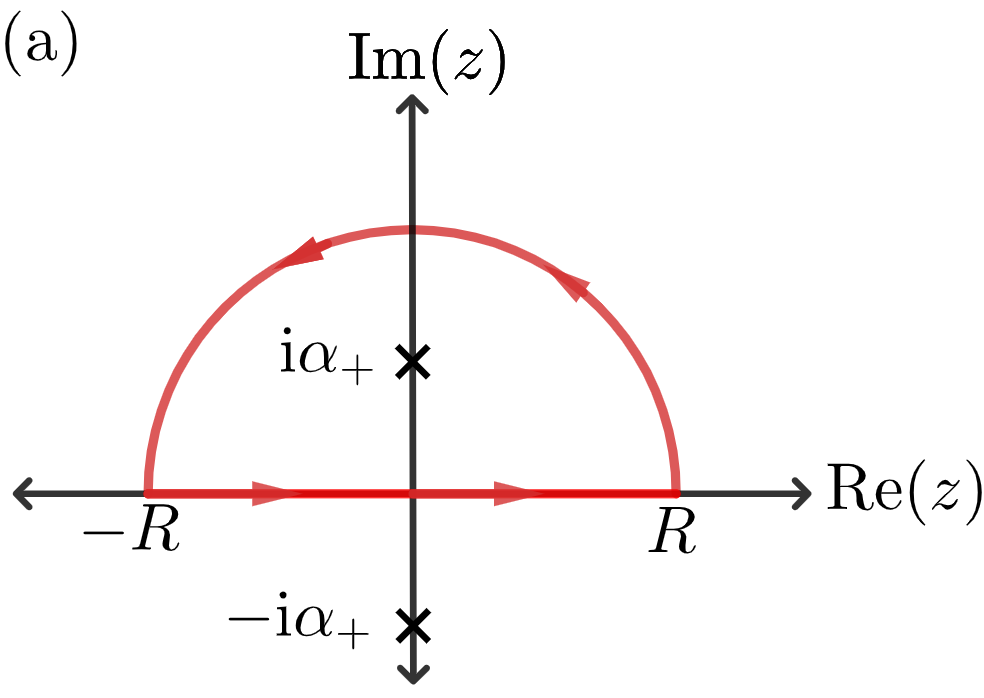
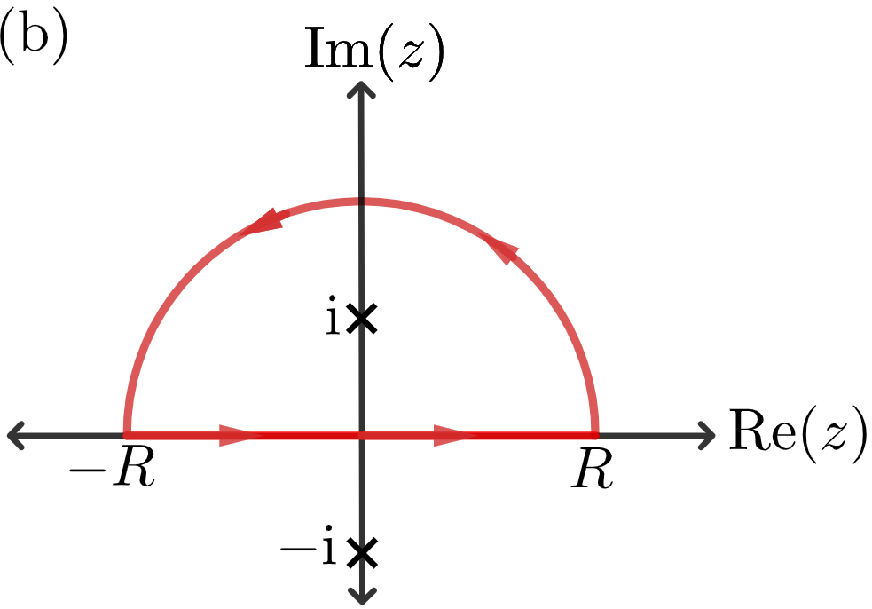
Figure 5: Contours for (a) the $x$-integration of $\mathcal{M}_{1}$, (b) the $y$-integration of $\mathcal{M}_{1}$

Then, it is straightforward to show that

$$\mathcal{M}_{1}=\frac{1}{16m^{3}}\int_{-\infty}^{+\infty}\frac{dy}{2\pi}\left[\frac{1}{(y^{2}+1)^{2}}+\frac{3(y^{2}-1)}{(y^{2}+1)^{3}}\right],$$ (93)

which can be easily computed with the contour of Fig. 5(b):

$$\mathcal{M}_{1}=-\frac{1}{128m^{3}}.$$ (94)

By collecting the results:

$$\lim_{\begin{subarray}{c}p_{0}\to 0\\ \mathbf{p}\to 0\end{subarray}}T_{1}^{\mu\nu}=-\frac{\mathrm{i}|q_{f}B|}{32\pi m}g_{\parallel}^{\mu\nu}.$$ (95)

C.2 Computing $T_{2}^{\mu\nu}$

In the limit $p_{0}=0,\mathbf{p}\to 0$:

$$\lim_{\begin{subarray}{c}p_{0}\to 0\\ \mathbf{p}\to 0\end{subarray}}T_{2(\text{a})}^{\mu\nu}=\lim_{\begin{subarray}{c}p_{0}\to 0\\ \mathbf{p}\to 0\end{subarray}}T_{2(\text{b})}^{\mu\nu},~{}\text{and}~{}\lim_{\begin{subarray}{c}p_{0}\to 0\\ \mathbf{p}\to 0\end{subarray}}T_{2(\text{c})}^{\mu\nu}=0,$$ (96)

then

$$\lim_{\begin{subarray}{c}p_{0}\to 0\\ \mathbf{p}\to 0\end{subarray}}T_{2}^{\mu\nu} = -\frac{16\mathrm{i}\pi|q_{f}B|}{(2\pi)^{2}}\int_{0}^{\infty}\frac{d\lambda}{(1+\lambda)^{2}}\int\frac{d^{2}\ell_{\parallel}}{(2\pi)^{2}}\frac{(\ell^{3})^{2}}{(\ell_{\parallel}^{2}-m^{2})^{2}\sqrt{l_{0}^{2}-m^{2}}}\left(g_{\parallel}^{\mu\nu}+2\delta_{3}^{\mu}\delta_{3}^{\nu}\right)$$ (97)

$$= -\frac{16\mathrm{i}\pi|q_{f}B|}{(2\pi)^{2}}\int\frac{d^{2}\ell_{\parallel}}{(2\pi)^{2}}\frac{(\ell^{3})^{2}}{(\ell_{\parallel}^{2}-m^{2})^{2}\sqrt{l_{0}^{2}-m^{2}}}\left(g_{\parallel}^{\mu\nu}+2\delta_{3}^{\mu}\delta_{3}^{\nu}\right).$$

Passing to the Euclidean space and defining $x$ and $y$ like in Eq. (90):

$$\lim_{\begin{subarray}{c}p_{0}\to 0\\ \mathbf{p}\to 0\end{subarray}}T_{2}^{\mu\nu} = -\frac{16\mathrm{i}\pi|q_{f}B|}{(2\pi)^{2}m}\int_{-\infty}^{+\infty}\frac{dy}{2\pi}\frac{1}{\sqrt{y^{2}+1}}\int_{-\infty}^{+\infty}\frac{dx}{2\pi}\frac{x^{2}}{(x^{2}+\alpha_{+}^{2})^{2}}\left(g_{\parallel}^{\mu\nu}+2\delta_{3}^{\mu}\delta_{3}^{\nu}\right),$$ (98)

so that using the integration contour of Fig. 5(a):

$$\int_{-\infty}^{+\infty}\frac{dx}{2\pi}\frac{x^{2}}{(x^{2}+\alpha_{+}^{2})^{2}}=\lim_{R\to\infty}\oint_{\mathcal{C}}\frac{dz}{2\pi}\frac{z^{2}}{(z^{2}+\alpha_{+}^{2})^{2}}=\mathrm{i}~{}\text{Res}\left[\frac{z^{2}}{(z^{2}+\alpha_{+}^{2})^{2}}\right]_{z=\mathrm{i}\alpha_{+}}=\frac{1}{4\alpha_{+}}=\frac{1}{4\sqrt{y^{2}+1}},$$ (99)

therefore

$$\lim_{\begin{subarray}{c}p_{0}\to 0\\ \mathbf{p}\to 0\end{subarray}}T_{2}^{\mu\nu} = -\frac{4\mathrm{i}\pi|q_{f}B|}{(2\pi)^{2}m}\int_{-\infty}^{+\infty}\frac{dy}{2\pi}\frac{1}{(y^{2}+1)}\left(g_{\parallel}^{\mu\nu}+2\delta_{3}^{\mu}\delta_{3}^{\nu}\right),$$ (100)

and after using the contour of Fig. 5(b):

$$\int_{-\infty}^{+\infty}\frac{dy}{2\pi}\frac{1}{(y^{2}+1)}=\lim_{R\to\infty}\oint_{\mathcal{C}}\frac{dz}{2\pi}\frac{1}{z^{2}+1}=\mathrm{i}~{}\text{Res}\left[\frac{1}{z^{2}+1}\right]_{z=\mathrm{i}}=\frac{1}{2},$$ (101)

so that

$$\lim_{\begin{subarray}{c}p_{0}\to 0\\ \mathbf{p}\to 0\end{subarray}}T_{2}^{\mu\nu} = -\frac{\mathrm{i}|q_{f}B|}{2\pi m}\left(g_{\parallel}^{\mu\nu}+2\delta_{3}^{\mu}\delta_{3}^{\nu}\right).$$ (102)

C.3 Computing $T_{3}^{\mu\nu}$

$$\lim_{\begin{subarray}{c}p_{0}\to 0\\ \mathbf{p}\to 0\end{subarray}}T_{3}^{\mu\nu} = \frac{16\mathrm{i}\pi|q_{f}B|}{3(2\pi)^{2}}\int_{0}^{\infty}\frac{d\lambda}{(1+\lambda)^{2}}\int\frac{d^{2}\ell_{\parallel}}{(2\pi)^{2}}\frac{\left(m^{2}-\ell_{\parallel}^{2}\right)\left(g_{\parallel}^{\mu\nu}-g_{\perp}^{\mu\nu}\right)+\ell_{\parallel}^{2}g_{\parallel}^{\mu\nu}}{(\ell_{\parallel}^{2}-m^{2})^{2}\sqrt{l_{0}^{2}-m^{2}}}$$ (103)

$$= \frac{16\mathrm{i}\pi|q_{f}B|}{3(2\pi)^{2}}\int\frac{d^{2}\ell_{\parallel}}{(2\pi)^{2}}\left[\frac{m^{2}}{(\ell_{\parallel}^{2}-m^{2})^{2}\sqrt{l_{0}^{2}-m^{2}}}g_{\parallel}^{\mu\nu}+\frac{\ell_{\parallel}^{2}-m^{2}}{(\ell_{\parallel}^{2}-m^{2})^{2}\sqrt{l_{0}^{2}-m^{2}}}g_{\perp}^{\mu\nu}\right]$$

$$= \frac{16\mathrm{i}\pi|q_{f}B|}{3(2\pi)^{2}}\int\frac{d^{2}\ell_{\text{E}}}{(2\pi)^{2}}\left[\frac{m^{2}}{(\ell_{\text{E}}+m^{2})^{2}\sqrt{l_{4}^{2}+m^{2}}}g_{\parallel}^{\mu\nu}-\frac{\ell_{\text{E}}^{2}+m^{2}}{(\ell_{\text{E}}+m^{2})^{2}\sqrt{l_{4}^{2}+m^{2}}}g_{\perp}^{\mu\nu}\right]$$

$$= \frac{16\mathrm{i}\pi|q_{f}B|}{3(2\pi)^{2}m}\int_{-\infty}^{+\infty}\frac{dy}{2\pi}\int_{-\infty}^{+\infty}\frac{dx}{2\pi}\left[\frac{1}{(x^{2}+y^{2}+1)^{2}\sqrt{y^{2}+1}}g_{\parallel}^{\mu\nu}-\frac{x^{2}+y^{2}+1}{(x^{2}+y^{2}+1)^{2}\sqrt{y^{2}+1}}g_{\perp}^{\mu\nu}\right]$$

We have the following integrals:

$$\int_{-\infty}^{+\infty}\frac{dy}{2\pi}\frac{1}{\sqrt{y^{2}+1}}\int_{-\infty}^{+\infty}\frac{dx}{2\pi}\frac{1}{(x^{2}+\alpha_{+}^{2})^{2}}=\frac{1}{4}\int_{-\infty}^{+\infty}\frac{dy}{2\pi}\frac{1}{(y^{2}+1)^{2}}=\frac{1}{16},$$ (104a)

and

$$\int_{-\infty}^{+\infty}\frac{dy}{2\pi}\frac{1}{\sqrt{y^{2}+1}}\int_{-\infty}^{+\infty}\frac{dx}{2\pi}\frac{x^{2}+y^{2}+1}{(x^{2}+\alpha_{+}^{2})^{2}}=\frac{1}{2}\int_{-\infty}^{+\infty}\frac{dy}{2\pi}\frac{1}{y^{2}+1}=\frac{1}{4}.$$ (104b)

Therefore:

$$\lim_{\begin{subarray}{c}p_{0}\to 0\\ \mathbf{p}\to 0\end{subarray}}T_{3}^{\mu\nu}=\frac{\mathrm{i}|q_{f}B|}{3\pi m}\left(\frac{1}{4}g_{\parallel}^{\mu\nu}-g_{\perp}^{\mu\nu}\right).$$ (105)

Appendix D Projections onto the standard tensor basis

The tensors $T_{i}^{\mu\nu}$ can be written as:

$$T_{1}^{\mu\nu}=\mathcal{I}_{1}(p)P_{\parallel}^{\mu\nu}+\mathcal{J}_{1}(p)g_{\parallel}^{\mu\nu},$$ (106a)

$$T_{2}^{\mu\nu}=\mathcal{I}_{2}(p)\left(g_{\parallel}^{\mu\nu}+2b^{\mu}b^{\nu}\right),$$ (106b)

$$T_{3}^{\mu\nu}=\mathcal{I}_{3}(p)P_{\parallel}^{\mu\nu}+\mathcal{J}_{3}(p)g_{\parallel}^{\mu\nu}+\mathcal{K}_{3}(p)g_{\perp}^{\mu\nu},$$ (106c)

where we defined the 4-vector $b^{\mu}=(0,0,0,1)$, the tensor

$$P_{\parallel}^{\mu\nu}=g_{\parallel}^{\mu\nu}-\frac{p_{\parallel}^{\mu}p_{\parallel}^{\nu}}{p_{\parallel}^{2}},$$ (107)

and the integrals

$$\mathcal{I}_{1}(p) = \frac{64\mathrm{i}\pi|q_{f}B|}{(2\pi)^{2}}p_{\parallel}^{2}\exp\left(-\frac{2\mathbf{p}_{\perp}^{2}}{3|q_{f}B|}\right)\int_{0}^{\infty}\frac{\lambda^{2}d\lambda}{(1+\lambda)^{5}}\int\frac{d^{2}\ell_{\parallel}}{(2\pi)^{2}}\frac{(1-\lambda)\ell_{\parallel}^{2}+\frac{\lambda^{2}}{(1+\lambda)^{2}}p_{\parallel}^{2}+m^{2}}{\left(\ell_{\parallel}^{2}+\frac{\lambda}{(1+\lambda)^{2}}p_{\parallel}^{2}-m^{2}\right)^{3}\sqrt{\left(l_{0}-\frac{\lambda}{1+\lambda}p_{0}\right)^{2}-m^{2}}}$$ (108a)

$$\mathcal{J}_{1}(p) = \frac{32\mathrm{i}\pi|q_{f}B|}{(2\pi)^{2}}p_{\parallel}^{2}\exp\left(-\frac{2\mathbf{p}_{\perp}^{2}}{3|q_{f}B|}\right)\int_{0}^{\infty}\frac{\lambda^{2}d\lambda}{(1+\lambda)^{5}}\int\frac{d^{2}\ell_{\parallel}}{(2\pi)^{2}}\frac{1}{\left(\ell_{\parallel}^{2}+\frac{\lambda}{(1+\lambda)^{2}}p_{\parallel}^{2}-m^{2}\right)^{3}\sqrt{\left(l_{0}-\frac{\lambda}{1+\lambda}p_{0}\right)^{2}-m^{2}}}$$ (108b)

$$\times \left[\left(\ell_{\parallel}^{2}+\frac{\lambda^{2}}{(1+\lambda)^{2}}p_{\parallel}^{2}+m^{2}\right)\left(m^{2}-\frac{\lambda}{(1+\lambda)^{2}}p_{\parallel}^{2}\right)-\frac{\lambda(1-\lambda)}{(1+\lambda)^{2}}p_{\parallel}^{2}\ell_{\parallel}^{2}\right],$$

$$\mathcal{I}_{2}(p) = \frac{16\mathrm{i}\pi|q_{f}B|}{(2\pi)^{2}}\exp\left(-\frac{2\mathbf{p}_{\perp}^{2}}{3|q_{f}B|}\right)\int_{0}^{\infty}\frac{d\lambda}{(1+\lambda)^{2}}\int\frac{d^{2}\ell_{\parallel}}{(2\pi)^{2}}\frac{-(\ell^{3})^{2}+\frac{\lambda}{(1+\lambda)^{2}}p_{3}^{2}}{\left(\ell_{\parallel}^{2}+\frac{\lambda}{(1+\lambda)^{2}}p_{\parallel}^{2}-m^{2}\right)^{2}\sqrt{\left(l_{0}-\frac{\lambda}{1+\lambda}p_{0}\right)^{2}-m^{2}}},$$ (108c)

$$\mathcal{I}_{3}(p) = \frac{16\mathrm{i}\pi|q_{f}B|}{3(2\pi)^{2}}p_{\parallel}^{2}\exp\left(-\frac{2\mathbf{p}_{\perp}^{2}}{3|q_{f}B|}\right)\int_{0}^{\infty}\frac{\lambda d\lambda}{(1+\lambda)^{4}}\int\frac{d^{2}\ell_{\parallel}}{(2\pi)^{2}}\frac{1}{\sqrt{\left(l_{0}^{2}+\frac{\lambda}{1+\lambda}p_{0}\right)^{2}-m^{2}}\left(\ell_{\parallel}^{2}+\frac{\lambda}{(1+\lambda)^{2}}p_{\parallel}^{2}-m^{2}\right)^{2}},$$ (108d)

$$\mathcal{J}_{3}(p) = \frac{16\mathrm{i}\pi|q_{f}B|}{3(2\pi)^{2}}\exp\left(-\frac{2\mathbf{p}_{\perp}^{2}}{3|q_{f}B|}\right)\int_{0}^{\infty}\frac{d\lambda}{(1+\lambda)^{2}}\int\frac{d^{2}\ell_{\parallel}}{(2\pi)^{2}}\frac{m^{2}-\frac{\lambda}{(1+\lambda)^{2}}p_{\parallel}^{2}}{\sqrt{\left(l_{0}^{2}+\frac{\lambda}{1+\lambda}p_{0}\right)^{2}-m^{2}}\left(\ell_{\parallel}^{2}+\frac{\lambda}{(1+\lambda)^{2}}p_{\parallel}^{2}-m^{2}\right)^{2}},$$ (108e)

$$\mathcal{K}_{3}(p) = -\frac{16\mathrm{i}\pi|q_{f}B|}{3(2\pi)^{2}}\exp\left(-\frac{2\mathbf{p}_{\perp}^{2}}{3|q_{f}B|}\right)\int_{0}^{\infty}\frac{d\lambda}{(1+\lambda)^{2}}\int\frac{d^{2}\ell_{\parallel}}{(2\pi)^{2}}\frac{m^{2}-\ell_{\parallel}^{2}+\frac{\lambda}{(1+\lambda)^{2}}p_{\parallel}^{2}}{\sqrt{\left(l_{0}^{2}+\frac{\lambda}{1+\lambda}p_{0}\right)^{2}-m^{2}}\left(\ell_{\parallel}^{2}+\frac{\lambda}{(1+\lambda)^{2}}p_{\parallel}^{2}-m^{2}\right)^{2}}.$$ (108f)

Let us assume that the full polarization tensor is written in the basis $\left\{P_{\parallel}^{\mu\nu},P_{\perp}^{\mu\nu},P_{0}^{\mu\nu}\right\}$, where

$$P_{\parallel}^{\mu\nu} \equiv g_{\parallel}^{\mu\nu}-\frac{p_{\parallel}^{\mu}p_{\parallel}^{\nu}}{p_{\parallel}^{2}}$$

$$P_{\perp}^{\mu\nu} \equiv g_{\perp}^{\mu\nu}+\frac{p_{\perp}^{\mu}p_{\perp}^{\nu}}{\mathbf{p}_{\perp}^{2}},$$

$$P_{0}^{\mu\nu} \equiv g^{\mu\nu}-\frac{p^{\mu}p^{\nu}}{p^{2}}-P_{\parallel}^{\mu\nu}-P_{\perp}^{\mu\nu},$$ (109)

so that

$$\mathrm{i}\Pi_{\Delta}^{\mu\nu}=\Pi_{\parallel}P_{\parallel}^{\mu\nu}+\Pi_{\perp}P_{\perp}^{\mu\nu}+\Pi_{0}P_{0}^{\mu\nu}.$$ (110)

Hence, given that

$$\mathrm{i}\Pi_{\Delta}^{\mu\nu} = \mathrm{i}\Pi_{0}^{\mu\nu}+\mathrm{i}\frac{q^{2}|q_{f}B|\Delta}{4\pi}\sum_{i=1}^{3}T_{i}^{\mu\nu}$$

$$= \mathrm{i}\frac{q^{2}|q_{f}B|}{4\pi^{2}}\Bigg{\{}\left[e^{-\frac{\mathbf{p}_{\perp}^{2}}{2|q_{f}B|}}p_{\parallel}^{2}\mathcal{I}_{0}+\Delta\left(\mathcal{I}_{1}+\mathcal{I}_{3}\right)\right]P_{\parallel}^{\mu\nu}.$$

$$+ \Delta\left(\mathcal{J}_{1}+\mathcal{I}_{2}+\mathcal{J}_{3}\right)g_{\parallel}^{\mu\nu}+\Delta\mathcal{K}_{3}g_{\perp}^{\mu\nu}+2\Delta\mathcal{I}_{2}b^{\mu}b^{\nu}\Bigg{\}},$$

it is straightforward to show that:

$$\Pi_{\parallel} = \mathrm{i}\frac{q^{2}|q_{f}B|}{4\pi}\Bigg{[}e^{-\frac{\mathbf{p}_{\perp}^{2}}{2|q_{f}B|}}p_{\parallel}^{2}\mathcal{I}_{0}+\Delta\left(\mathcal{I}_{1}+\mathcal{I}_{3}\right)-\frac{2\Delta p_{0}^{2}}{p_{\parallel}^{2}}\mathcal{I}_{2}$$

$$+ \Delta\left(\mathcal{J}_{1}+\mathcal{I}_{2}+\mathcal{J}_{3}\right)\Bigg{]},$$

$$\Pi_{\perp}=\mathrm{i}\frac{q^{2}|q_{f}B|}{4\pi}\Delta\mathcal{K}_{3},$$ (112b)

and

$$\Pi_{0} = \mathrm{i}\frac{q^{2}|q_{f}B|}{4\pi}\Bigg{[}-\frac{\mathbf{p}_{\perp}^{2}}{p^{2}}\Delta\left(\mathcal{J}_{1}+\mathcal{I}_{2}+\mathcal{J}_{3}\right)+\frac{p_{\parallel}^{2}}{p^{2}}\Delta\mathcal{K}_{3}$$ (112c)

$$+ 2\Delta\left(\frac{p_{0}^{2}}{p_{\parallel}^{2}}-\frac{p_{3}^{2}}{p^{2}}-1\right)\mathcal{I}_{2}\Bigg{]},$$

provided by the fact that the basis is orthonormal and

$$P_{\parallel}^{\mu\nu}g_{\mu\nu}^{\parallel}=1$$ (113a)

$$P_{\parallel}^{\mu\nu}b_{\mu}b_{\nu}=-\frac{p_{0}^{2}}{p_{\parallel}^{2}}$$ (113b)

$$P_{\perp}^{\mu\nu}g_{\mu\nu}^{\perp}=1$$ (113c)

$$P_{0}^{\mu\nu}g_{\mu\nu}^{\parallel}=-\frac{\mathbf{p}_{\perp}^{2}}{p^{2}}$$ (113d)

$$P_{0}^{\mu\nu}b_{\mu}b_{\nu}=\frac{p_{0}^{2}}{p_{\parallel}^{2}}-\frac{p_{3}^{2}}{p^{2}}-1,$$ (113e)

and

$$P_{0}^{\mu\nu}g_{\mu\nu}^{\perp}=\frac{p_{\parallel}^{2}}{p^{2}}.$$ (113f)