Towards a more complete description of hybrid leptogenesis

Abstract

Hybrid leptogenesis framework combining type I and type II seesaw mechanism for neutrino mass necessarily include scattering topologies involving both the scalar triplet and the right handed neutrino. We demonstrate that a systematic inclusion of these mixed scatterings can significantly alter the evolution of the number densities leading to an order of magnitude change in the predicted value of present-day asymmetry. We provide quantitative limit on the degeneracy of the seesaw scales where the complete analysis becomes numerically significant, limiting the validity of leptogenesis being dominated by the lightest seesaw species.

1 Introduction

Generating the observed Baryon Asymmetry of the Universe (BAU) through leptogenesis has been widely discussed in the literature as it provides a possible connection between the eluding enigmas of the neutrino mass and the matter-antimatter asymmetry Fukugita:1986hr ; Davidson:2008bu ; DiBari:2021fhs . In this context the seesaw models that provides a natural framework for generating tiny masses for the neutrinos are of interest as they can also provide an handle to drive leptogenesis through CP violating out-of-equilibrium decays of the heavy seesaw states of different types King:2003jb ; deGouvea:2016qpx ; Cai:2017jrq ; Ma:2006km , viz the right handed neutrino(s) for the Type I Mohapatra:1979ia ; Schechter:1980gr , scalar triplet(s) for Type II Lazarides:1980nt ; Mohapatra:1986bd and the fermionic triplet(s) for Type III Foot:1988aq seesaw mechanism.

In general if there are a number of heavy species (of single type) with hierarchical masses that contribute to leptogenesis, the washout effects imply that the final asymmetry is dominated by the lightest species, see Engelhard:2006yg for exceptions. The same is true for a mixed mode of leptogenesis where heavy hierarchical species of different types or categories contribute toward leptogenesis. Interestingly as the scales start coming close, processes that include participation of more than one type of these heavy species also becomes important (henceforth called mixed processes) and consequently, estimation of the asymmetry requires a detailed study of the coupled Boltzmann equations including all the relevant states. In this work we present a hybrid scenario with Type I and Type II seesaw states simultaneously contributing to the neutrino mass and leptogenesis. We focus on the region of parameter space, in consonance with the neutrino oscillation data, where the mixed processes involving topologies with states belonging to the two different seesaw frameworks become comparable ($i.e.$ numerically significant). We show that the full analysis including all sorts of relevant species in this case can significantly differ from the approximate asymmetries obtained by assuming the dominant role to be played by the lightest state only.

The minimal version of this hybrid leptogenesis framework considered in this work is based on an extension of the Standard Model (SM) by one $SU(2)_{L}$ triplet scalar having hypercharge $Y=1$ in the scalar sector while the fermionic sector is augmented with a single right handed neutrino (RHN). In general, the appearance of both RHN(s) and triplet(s) occur naturally in several extensions of SM such as the left-right symmetric model (LRSM) Pati:1974yy ; Mohapatra:1974gc and grand unified theories (GUTs) Georgi:1974sy ; Georgi:1974yf ; Fritzsch:1974nn ; Langacker:1980js ; Ibarra:2018dib ; Bhattacharya:2021jli . The seesaw neutrino masses in agreement with the experimental limits can be generated by combining the type I and type II seesaw contributions Esteban:2020cvm . The minimality of the framework ensures that the CP violating decays of heavy state(s) necessarily requires the simultaneous involvement of scalar triplet as well the right handed neutrino to generate the primordial matter-antimatter asymmetry. Study of leptogenesis in these models have been carried out in the literature where being hierarchical in nature, decay of the lightest state (either the RHN or the triplet) turns out to be crucial in explaining the BAU via leptogenesis guided by the type I or II dominance in neutrino mass generation Babu:2005bh ; Akhmedov:2006yp ; Rink:2020uvt ; Hambye:2003ka ; Datta:2021gyi . However, in this work, we present for the first time a systematic analysis involving both the RHN and the scalar triplet contributing toward leptogenesis due to their closeness in mass-scales that finally leads to a substantial change in final baryon asymmetry estimation. In particular, we show that there are new $\Delta L=1\,\&\,2$ scattering processes in this simplified scenario of hybrid leptogenesis (involving both RHN and triplet) which are operative in the region where the type I and type II mass scales are relatively close and can significantly alter the baryon asymmetry parameter. As proof of principle, we present a couple of benchmark parameter points to demonstrate this finding. We also provide a quantitative constraint on the closeness of mass scales in terms of a degeneracy parameter where these processes with mixed topologies become numerically significant.

The paper is organized as follows. In section 2 we introduce the minimal model where the neutrino masses are generated from a combination of type I and type II seesaw mechanisms. We show the possibility of leptogenesis and the importance of hybrid processes in this framework with the results in section 3 before finally concluding in section 6.

2 The hybrid seesaw model and Neutrino mass

In this section we present the minimal extension of the SM which generate neutrino masses and drive leptogenesis within the hybrid type I + II seesaw framework. The SM is extended with a $SU(2)_{L}$ singlet RHN $(N_{R})$ and a complex scalar triplet $(\Delta)$ with hypercharge $Y=1$ which are responsible to generate tiny neutrino masses in type I and type II seesaw mechanisms respectively. The usual Yukawa interactions of the model are given by the two seesaw framework

$$-\mathcal{L}_{Y}={\mathcal{Y}_{N}}_{\alpha}\overline{L_{\alpha}}\widetilde{H}N_{R}+\dfrac{1}{2}{\mathcal{Y}_{\Delta}}_{\alpha\beta}\overline{L_{\alpha}^{c}}\Delta L_{\beta}+\dfrac{1}{2}M_{N}\overline{N_{R}}{N_{R}}^{c}+\text{ h.c.}\ ,$$ (1)

with $\widetilde{H}=i\sigma_{2}H^{*}$ where $L_{\alpha}$ and $\widetilde{H}$ denotes the SM leptons and Higgs doublet respectively and $\alpha,\beta=1,2,3$ are flavour indices. The Yukawa couplings of the RHN is denoted by ${\mathcal{Y}_{N}}_{\alpha}$ with $6$ independent real elements, on the other hand for the scalar triplet the Yukawas are given by a $3\times 3$ dimensional complex symmetric matrix $\mathcal{Y}_{\Delta}$ with $9$ independent elements. The scalar potential of this hybrid scenario is identical to a pure type II seesaw with only one triplet and be represented by

$$V(H,\Delta) = -\ m^{2}_{H}(H^{\dagger}H)+\frac{\lambda}{4}(H^{\dagger}H)^{2}+M_{\Delta}^{2}\text{Tr}(\Delta^{\dagger}\Delta)+\lambda_{2}\left[\text{Tr}(\Delta^{\dagger}\Delta)\right]^{2}+\lambda_{3}\text{Tr}(\Delta^{\dagger}\Delta)^{2}$$ (2)

$$+\ \lambda_{1}(H^{\dagger}H)\text{Tr}(\Delta^{\dagger}\Delta)+\lambda_{4}(H^{\dagger}\Delta\Delta^{\dagger}H)+\mu\left[H^{\mathsf{T}}i\tau_{2}\Delta^{\dagger}H+\text{ h.c.}\right]\ ,$$

where $\mu$ is the only dimension full trilinear coupling present in the theory. After the electroweak symmetry breaking (EWSB), the Higgs acquires a vacuum expectation value $(v_{H})$ which induces a tiny vev of the triplet given by $v_{\Delta}=\dfrac{1}{\sqrt{2}}\ \mu\left(\dfrac{v_{H}}{M_{\Delta}}\right)^{2}$ the value of which has an upper bound from precision electroweak measurements ParticleDataGroup:2022pth .

Note that the bare mass term $(M_{N})$ of $N_{R}$ present in eq. 1 and the trilinear coupling $(\mu)$ of $\Delta$ given in eq. 2 are chosen to be real without any loss of generality. The mass of the SM neutrinos are generated through a combination of type II and type I seesaw mechanisms given by

$$M_{\nu}=M_{\nu}^{II}+M_{\nu}^{I}=\dfrac{1}{\sqrt{2}}\mathcal{Y}_{\Delta}v_{\Delta}-\dfrac{v_{H}^{2}}{2M_{N}}\mathcal{Y}_{N}\mathcal{Y}_{N}^{\mathsf{T}}\ .$$ (3)

Note that the presence of a single RHN is not enough to construct a neutrino mass matrix, the diagonalisation of which can successfully describe both the solar and atmospheric mass differences. In this context, the inclusion of the triplet is a welcome feature. Contrarily, the type-II seesaw mechanism with single triplet although can satisfy the neutrino oscillation data by itself Esteban:2020cvm (due to the presence of a larger number of free parameters in the Yukawa matrix $\mathcal{Y}_{\Delta}$), it fails to generate any CP asymmetry in the decay of the single $\Delta$. Thus, in the simplified setup, presence of both the heavy states is crucial to fulfil the necessary requirements to simultaneously satisfy the neutrino oscillation data and generation of lepton asymmetry, which we demonstrate in the following section 3.

3 Leptogenesis in the minimal hybrid seesaw model

The study of Cosmic Microwave Background Radiation quantifies the present day abundance of baryon asymmetry as

$$Y_{\delta B}=8.750\pm 0.077\times 10^{-11}\ ,$$ (4)

observed by Planck Planck:2018vyg . Such an asymmetry can be generated by various mechanisms such as GUT baryogenesis Ignatiev:1978uf ; Yoshimura:1978ex ; Toussaint:1978br ; Dimopoulos:1978kv ; Ellis:1978xg ; Weinberg:1979bt ; Yoshimura:1979gy ; Barr:1979ye ; Nanopoulos:1979gx ; Yildiz:1979gx , Affleck-Dine mechanism Affleck:1984fy ; Dine:1995kz , electroweak baryogenesis Rubakov:1996vz ; Riotto:1999yt ; Cline:2006ts and baryogenesis via leptogenesis Riotto:1999yt ; Pilaftsis:1997jf ; Buchmuller:2004nz ; Buchmuller:2005eh ; Abada:2006ea ; Davidson:2008bu ; DiBari:2015oca . We focus here on the leptogenesis scenario where a lepton asymmetry is created by the out of equilibrium decays of both the RHN and a scalar triplet in the context of a minimal Type-I + II scenario as stated above, which finally would be converted into baryon asymmetry via the sphaleron process Khlebnikov:1988sr . A systematic evaluation of such asymmetry is discussed in the following subsections.

3.1 CP asymmetry generation

In the minimal hybrid seesaw construction, the involvement of two heavy seesaw states, $i.e.$ the RHN and the scalar, indicates that the initial lepton asymmetry can be contributed by the out of equilibrium decays of each of them in general. The interference between the tree level (figure 1(a)) and triplet mediated one loop (Figure 1(b)) decays of $N_{R}$ generate the CP asymmetry as given by Pramanick:2022put ; Hambye:2003ka

(a)

(b)

Figure 1: Tree level (left) and triplet mediated one loop level (right) decay of RHN generating the asymmetry parameter $\epsilon_{N}$ .

The RHN decays into a lepton and Higgs as denoted in figure 1. Crucially the interference between the tree level (figure 1(a)) and triplet mediated one loop level (figure 1(b)) diagrams generate the asymmetry of $N_{R}$ decay given by Pramanick:2022put ; Hambye:2003ka

$$\epsilon_{N} = \sum_{\alpha}\dfrac{\Gamma(N\rightarrow L_{\alpha}+H)-\Gamma(N\rightarrow\overline{L_{\alpha}}+\overline{H})}{\Gamma(N\rightarrow L_{\alpha}+H)+\Gamma(N\rightarrow\overline{L_{\alpha}}+\overline{H})}$$ (5)

$$= -\dfrac{1}{16\pi^{2}\Gamma_{N}}\sum_{\alpha,\beta}\mathfrak{Im}\big{[}{\mathcal{Y}_{N}}_{\alpha}\ {\mathcal{Y}_{N}}_{\beta}\ {\mathcal{Y}_{\Delta}^{*}}_{\alpha\beta}\ \mu\big{]}\bigg{[}1-\dfrac{M_{\Delta}^{2}}{M_{N}^{2}}\log\left(1+\dfrac{M_{N}^{2}}{M_{\Delta}^{2}}\right)\bigg{]}\ .$$

(a)

(b)

Figure 2: Tree level (left) and RHN mediated one loop level (right) decay of triplet generating the asymmetry parameter $\epsilon_{\Delta}$ .

On the other hand, the CP asymmetry from the decay of the triplet results from the interference between the tree (figure 2(a)) and one loop (figure 2(b)) diagrams and is given by Pramanick:2022put ; Hambye:2003ka

$$\epsilon_{\Delta} = \sum_{\alpha,\beta}\dfrac{\Gamma(\overline{\Delta}\rightarrow L_{\alpha}+L_{\beta})-\Gamma(\Delta\rightarrow\overline{L_{\alpha}}+\overline{L_{\beta}})}{\Gamma(\overline{\Delta}\rightarrow L_{\alpha}+L_{\beta})+\Gamma(\Delta\rightarrow\overline{L_{\alpha}}+\overline{L_{\beta}})}$$ (6)

$$= \dfrac{1}{64\pi^{2}\Gamma_{\Delta}}\sum_{\alpha,\beta}\mathfrak{Im}\big{[}{\mathcal{Y}_{N}^{*}}_{\alpha}\ {\mathcal{Y}_{N}^{*}}_{\beta}\ {\mathcal{Y}_{\Delta}}_{\alpha\beta}\ \mu\big{]}\bigg{[}\dfrac{M_{N}}{M_{\Delta}}\log\left(1+\dfrac{M_{\Delta}^{2}}{M_{N}^{2}}\right)\bigg{]}\ .$$

In the above expression, $\Gamma_{N}$ and $\Gamma_{\Delta}$ denote the total decay width of RHN and triplet respectively and given by

$$\Gamma_{N}=\dfrac{M_{N}}{8\pi}\text{Tr}\left({\mathcal{Y}_{N}}^{\dagger}\mathcal{Y}_{N}\right)\ ;\quad\Gamma_{\Delta}=\dfrac{M_{\Delta}}{8\pi}\Bigg{[}\text{Tr}\left({\mathcal{Y}_{\Delta}}^{\dagger}\mathcal{Y}_{\Delta}\right)+\left(\dfrac{\mu}{M_{\Delta}}\right)^{2}\Bigg{]}\ .$$ (7)

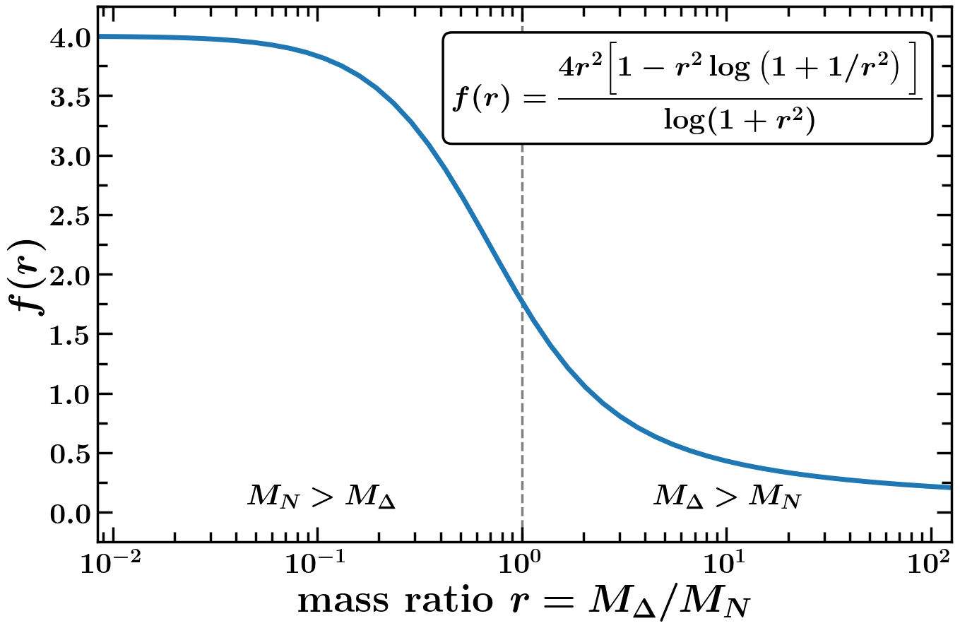
(a)

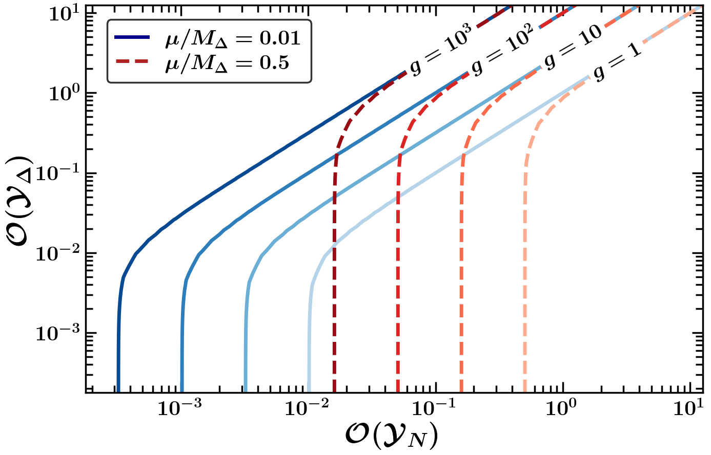
(b)

Figure 3: Left panel shows the variation of $f(r)$ defined in eq. 8 with respect to the mass ratio $r$ where mass degeneracy of RHN and triplet is denoted via the vertical gray dashed line. Right panel shows order of magnitude contours of $g(\mathcal{Y}_{N},\mathcal{Y}_{\Delta},\mu/M_{\Delta})$ appearing in eq. 8 in the plane of Yukawa couplings $\mathcal{O}(\mathcal{Y}_{N})$ vs. $\mathcal{O}(\mathcal{Y}_{\Delta})$ for fixed value of $\mu/M_{\Delta}=0.01(0.5)$ denoted by solid (dashed) blue (red) curves.

In this simplified setup, it is interesting to note that the combination of the neutrino Yukawas and trilinear couplings that appear in the expression of $\epsilon_{N}$ and $\epsilon_{\Delta}$ in eqs. 5 and 6 respectively are complex conjugates of each other. Thus the contribution of this specific combination cancels out in the expression of the ratio of the CP asymmetry parameters defined as $\epsilon_{r}=\epsilon_{N}/\epsilon_{\Delta}$, representative of a relative hierarchy between the CP asymmetries generated from RHN and Triplet decays. Apart from the couplings involved, the triplet to RHN mass ratio defined by $r=M_{\Delta}/M_{N}$ also plays a significant role in determining $\epsilon_{r}$. In order to extract the effects of various couplings and the masses in the asymmetry parameter, the ratio $\epsilon_{r}$ can be factorized as

$$\epsilon_{r} =\Big{[}\dfrac{4r^{2}\left(1-r^{2}\log(1+1/r^{2})\right)}{\log(1+r^{2})}\Big{]}\Big{[}\dfrac{\text{Tr}\left(\mathcal{Y}_{\Delta}^{\dagger}\mathcal{Y}_{\Delta}\right)+\left(\dfrac{\mu}{M_{\Delta}}\right)^{2}}{\text{Tr}\left(\mathcal{Y}_{N}^{\dagger}\mathcal{Y}_{N}\right)}\Big{]}$$ (8)

$$\equiv f(r)\ g(\mathcal{Y}_{N},\mathcal{Y}_{\Delta},\mu/M_{\Delta}),$$

where the functions $f(r)$ and $g(\mathcal{Y}_{N},\mathcal{Y}_{\Delta},\mu/M_{\Delta})$ encapsulate the dependence on mass ratio $r=M_{\Delta}/M_{N}$ and various couplings respectively. In order to exhibit such dependence more explicitly, we include figures 3(a) and 3(b). As can be seen from it, the mass ratio dependent factor $f(r)$ appearing in eq. 8 attains a maximum value $4.0$ corresponding to a smaller value of $r\sim\mathcal{O}(10^{-2})$ while it asymptotically approaches zero for larger value of $r\gg 1$. On the other hand, a contour plot for function $g$ is drawn in $\mathcal{Y}_{N}-\mathcal{Y}_{\Delta}$ plane for some fixed values of $g$ and $\mu/M_{\Delta}$ in figure 3(b). As evident, a relatively large (or small) value of $g$ or initial relative asymmetry between RHN or triplet decay is obtainable by appropriately tuning the quantities $\mu/M_{\Delta}$ and/or hierarchy between couplings $\mathcal{Y}_{N}$ and $\mathcal{Y}_{\Delta}$.

3.2 Evolution of baryon asymmetry

In this section we discuss how the primordial lepton asymmetry originated due to the decay of heavy seesaw states can be associated with the present day observation of BAU Planck:2018vyg . In order to investigate the evolution of $B-L$ asymmetry through the out of equilibrium decay of heavier species, we need to solve the set of coupled Boltzmann equations (BEs) associated with abundances of various particles. This $B-L$ asymmetry can then be transferred to a net baryon asymmetry $(B)$ through non perturbative sphaleron processes Khlebnikov:1988sr . The sphaleron factor in this model can be calculated to be $a_{\text{sph}}=12/37$ assuming sphaleron remains at equilibrium after EW phase transition Harvey:1990qw and the baryon asymmetry can be expressed as the $B-L$ asymmetry as $Y_{\delta B}=a_{\text{sph}}\cdot Y_{\delta(B-L)}$.

We consider Yukawa couplings in the range of $\mathcal{O}(10^{-3}-10^{-1})$ for both RHN and scalar triplet while being in alignment with the seesaw spirit which fixes the mass of these heavy particles to be greater than $10^{12}$ GeV. This high scale of leptogenesis can be safely considered to be unflavoured as none of the SM Yukawa interactions enter thermal equilibrium at these temperatures.

In order to write down the BEs for this mixed seesaw framework, one needs to track down the abundance of RHN, triplet (both its symmetric and asymmetric part denoted by $\Sigma\Delta=\Delta+\overline{\Delta}$ and $\delta\Delta=\Delta-\overline{\Delta}$ respectively) and the $B-L$ asymmetry which forms a set of four coupled differential equations given by

$$\dot{Y}_{N}={} -\left(\dfrac{Y_{N}}{Y_{N}^{\text{eq}}}-1\right)\Bigg{[}\gamma_{D_{N}}+2\Big{(}\gamma^{NL}_{\overline{Q}t_{R}}+\gamma^{NQ}_{Lt_{R}}+\gamma^{N\overline{t_{R}}}_{L\overline{Q}}\Big{)}\Bigg{]}$$

$$-\ 2\Bigg{[}\left(\dfrac{Y_{N}}{Y_{N}^{\text{eq}}}\dfrac{Y_{\Sigma\Delta}}{Y_{\Sigma\Delta}^{\text{eq}}}-1\right)\gamma^{\Delta N}_{\overline{L}H}+\left(\dfrac{Y_{N}}{Y_{N}^{\text{eq}}}-\dfrac{Y_{\Sigma\Delta}}{Y_{\Sigma\Delta}^{\text{eq}}}\right)\bigg{(}\gamma^{\Delta\overline{H}}_{\overline{L}N}+\gamma^{\Delta L}_{HN}\bigg{)}\Bigg{]}\ ,$$ (9a)

$$\dot{Y}_{\Sigma\Delta}={} -\left(\dfrac{Y_{\Sigma\Delta}}{Y_{\Sigma\Delta}^{\text{eq}}}-1\right)\gamma_{D_{\Delta}}-2\left\{\left(\dfrac{Y_{\Sigma\Delta}}{Y_{\Sigma\Delta}^{\text{eq}}}\right)^{2}-1\right\}\gamma_{A}$$

$$-\ 2\Bigg{[}\left(\dfrac{Y_{N}}{Y_{N}^{\text{eq}}}\dfrac{Y_{\Sigma\Delta}}{Y_{\Sigma\Delta}^{\text{eq}}}-1\right)\gamma^{\Delta N}_{\overline{L}H}+\left(\dfrac{Y_{\Sigma\Delta}}{Y_{\Sigma\Delta}^{\text{eq}}}-\dfrac{Y_{N}}{Y_{N}^{\text{eq}}}\right)\bigg{(}\gamma^{\Delta\overline{H}}_{\overline{L}N}+\gamma^{\Delta L}_{HN}\bigg{)}\Bigg{]}\ ,$$ (9b)

$$\dot{Y}_{\delta\Delta}={} -\left(\dfrac{Y_{\delta\Delta}}{Y_{\Sigma\Delta}^{\text{eq}}}+B_{L}\dfrac{Y_{\delta L}}{Y_{L}^{\text{eq}}}-B_{H}\dfrac{Y_{\delta H}}{Y_{H}^{\text{eq}}}\right)\gamma_{D_{\Delta}}$$

$$-\Bigg{[}\left(2\dfrac{Y_{\delta\Delta}}{Y_{\Sigma\Delta}^{\text{eq}}}\dfrac{Y_{N}}{Y_{N}^{\text{eq}}}+\dfrac{Y_{\delta L}}{Y_{L}^{\text{eq}}}-\dfrac{Y_{\delta H}}{Y_{H}^{\text{eq}}}\right)\gamma^{\Delta N}_{\overline{L}H}+\left(2\dfrac{Y_{\delta\Delta}}{Y_{\Sigma\Delta}^{\text{eq}}}-\dfrac{Y_{\delta H}}{Y_{H}^{\text{eq}}}+\dfrac{Y_{\delta L}}{Y_{L}^{\text{eq}}}\dfrac{Y_{N}}{Y_{N}^{\text{eq}}}\right)\gamma^{\Delta\overline{H}}_{\overline{L}N}$$

$$\hskip 11.38092pt+\left(2\dfrac{Y_{\delta\Delta}}{Y_{\Sigma\Delta}^{\text{eq}}}+\dfrac{Y_{\delta L}}{Y_{L}^{\text{eq}}}-\dfrac{Y_{\delta H}}{Y_{H}^{\text{eq}}}\dfrac{Y_{N}}{Y_{N}^{\text{eq}}}\right)\gamma^{\Delta L}_{HN}\Bigg{]}\ ,$$ (9c)

$$\dot{Y}_{\delta(B-L)}={} -\left(\dfrac{Y_{N}}{Y_{N}^{\text{eq}}}-1\right)\epsilon_{N}\gamma_{D_{N}}+2\left(\dfrac{Y_{\delta L}}{Y_{L}^{\text{eq}}}+\dfrac{Y_{\delta H}}{Y_{H}^{\text{eq}}}\right)\gamma_{D_{N}}$$

$$-\dfrac{1}{2}\left(\dfrac{Y_{\Sigma\Delta}}{Y_{\Sigma\Delta}^{\text{eq}}}-1\right)\epsilon_{\Delta}\gamma_{D_{\Delta}}+B_{L}\left(\dfrac{Y_{\delta\Delta}}{Y_{\Sigma\Delta}^{\text{eq}}}+\dfrac{Y_{\delta L}}{Y_{L}^{\text{eq}}}\right)\gamma_{D_{\Delta}}$$

$$+\dfrac{Y_{\delta L}}{Y_{L}^{\text{eq}}}\Bigg{[}\left(\gamma^{NQ}_{Lt_{R}}+\gamma^{N\overline{t_{R}}}_{L\overline{Q}}\right)-\dfrac{Y_{N}}{Y_{N}^{\text{eq}}}\ \gamma^{NL}_{\overline{Q}t_{R}}\Bigg{]}+2\left(\dfrac{Y_{\delta L}}{Y_{L}^{\text{eq}}}+\dfrac{Y_{\delta H}}{Y_{H}^{\text{eq}}}\right)\Big{(}{\gamma_{\text{\tiny RIS}}}^{L\,H}_{\overline{L}\,\overline{H}}+{\gamma_{\text{\tiny RIS}}}^{L\,L}_{\overline{H}\,\overline{H}}\Big{)}$$

$$+\Bigg{[}\left(2\dfrac{Y_{\delta\Delta}}{Y_{\Sigma\Delta}^{\text{eq}}}\dfrac{Y_{N}}{Y_{N}^{\text{eq}}}+\dfrac{Y_{\delta L}}{Y_{L}^{\text{eq}}}-\dfrac{Y_{\delta H}}{Y_{H}^{\text{eq}}}\right)\gamma^{\Delta N}_{\overline{L}H}+\left(2\dfrac{Y_{\delta\Delta}}{Y_{\Sigma\Delta}^{\text{eq}}}-\dfrac{Y_{\delta H}}{Y_{H}^{\text{eq}}}+\dfrac{Y_{\delta L}}{Y_{L}^{\text{eq}}}\dfrac{Y_{N}}{Y_{N}^{\text{eq}}}\right)\gamma^{\Delta\overline{H}}_{\overline{L}N}$$

$$\hskip 11.38092pt+\left(2\dfrac{Y_{\delta\Delta}}{Y_{\Sigma\Delta}^{\text{eq}}}+\dfrac{Y_{\delta L}}{Y_{L}^{\text{eq}}}-\dfrac{Y_{\delta H}}{Y_{H}^{\text{eq}}}\dfrac{Y_{N}}{Y_{N}^{\text{eq}}}\right)\gamma^{\Delta L}_{HN}\Bigg{]}\ ,$$ (9d)

where we follow usual notations and conventions which are elaborated in appendix A. The number density is denoted by $Y_{X}=n_{X}/s$ which is the ratio of the comoving number density $(n_{X})$ and entropy density $(s)$ for any species $X$ and is a function of the temperature $(T)$ and parameterized as the independent dimensionless variable $z=M_{N}/T$. The left hand side of these differential equations denote the change in the number density of $X$ which is defined as $\dot{Y}_{X}=z\ s(z)\ H(z)\ dY_{X}/dz$ where $X=N,\Sigma\Delta,\delta\Delta$ and $\delta(B-L)$ and $H(z)$ is the Hubble parameter. $B_{L}$ and $B_{H}$ are the branching ratios of the triplet decaying into lepton and Higgs respectively (given in 11) whereas the superscript ‘eq’ denotes the equilibrium number density of any given species. The asymmetry in the abundance of SM lepton doublet $(Y_{\delta L})$ and Higgs doublet $(Y_{\delta H})$ are linearly dependent on $Y_{\delta\Delta}$ and $Y_{\delta(B-L)}$ and can be expressed in terms of $C_{L}$ and $C_{H}$ coefficient matrices Barbieri:1999ma ; Nardi:2005hs ; Abada:2006fw ; Sierra:2014tqa calculated from equilibration of chemical potentials in the temperature range $T\in\left[10^{12},10^{15}\right]$ GeV, applicable to our case.

The reaction density for a generic process is denoted as $\gamma^{X}_{Y}\equiv\gamma(X\rightarrow Y)$ where $X$ is single (two) particle initial state for decay ($2\leftrightarrow 2$ scattering) processes considered in the above set of coupled differential equations. The decay reaction densities of RHN and triplet are denoted by $\gamma_{D_{N}}$ and $\gamma_{D_{\Delta}}$ respectively which also act as source terms (proportional to $\epsilon_{N}$ and $\epsilon_{\Delta}$) in the evolution of $B-L$ asymmetry. Also, the real intermediate state (RIS) subtracted reaction densities are denoted as $\gamma_{\text{\tiny RIS}}$ for $\Delta L=2$ processes as discussed later and all of the reaction densities for various processes are explicitly summarized in appendix B. In passing we note that we do not include any decay or scattering process that involves three or more particles in the initial or final state Nardi:2007jp and also exclude gauge interactions related to pure type I seesaw which involves thermal corrections to masses of gauge bosons and other particles Giudice:2003jh . In the following we list down various processes and the corresponding reaction densities relevant for this hybrid framework.

$\bullet$ Decays of RHN and triplet:

The RHN decays into a lepton and a Higgs, whereas the triplet can decay into a lepton pair of a Higgs pair as shown in figure 1 and 2 respectively. Both the decay processes violate lepton number and the associated reaction densities for RHN and triplet decay are respectively given as

$$\gamma_{D_{N}}=n_{N}^{\text{eq}}\dfrac{K_{1}(z)}{K_{2}(z)}\Gamma_{N}\ ;\quad\gamma_{D_{\Delta}}=n_{\Sigma\Delta}^{\text{eq}}\dfrac{K_{1}(z)}{K_{2}(z)}\Gamma_{\Delta}\ ,$$ (10)

where $K_{n}(z)$ indicated the $n$-th order of second kind of Bessel function. The common factor appearing in both of the expressions is known as the dilution factor Buchmuller:2004nz due to the expansion of the universe. $\Gamma_{N}$ and $\Gamma_{\Delta}$ denotes the total decay width of RHN and triplet respectively and given by eq. 7. Also as the triplet can have two decay modes, the branching ratios of $\Delta$ decaying into a lepton pair and a Higgs pair are respectively given by $B_{L}$ and $B_{H}$ as

$$B_{L}=\dfrac{M_{\Delta}}{8\pi\Gamma_{\Delta}}\text{Tr}\left({\mathcal{Y}_{\Delta}}^{\dagger}\mathcal{Y}_{\Delta}\right)\ ;\quad B_{H}=\dfrac{\mu^{2}}{8\pi M_{\Delta}\Gamma_{\Delta}}\ .$$ (11)

$\bullet$ Scattering processes: ${\Delta L=1}$

The $\Delta L=1$ scattering process can be broadly divided into two classes, one that is already present in the pure type I seesaw framework and the other is only possible in the mixed type I + II seesaw scenario. The usual processes have one Yukawa interaction with $N_{R}$ in one vertex while the other vertex involves the Yukawa interaction of the top quark. There are three such processes out of which one is mediated by s-channel Higgs exchange and the other two are t-channel processes shown in figure 4 and the squared amplitudes of these processes are given in appendix B.1.

Figure 4: $2\leftrightarrow 2$ scattering processes $(\Delta L=1)$ involving top quark

On the other hand, there are also three additional processes which involve both $N_{R}$ and $\Delta$ in the external legs and are only possible in this hybrid seesaw framework. They constitute the mixed topology processes that we include in the analysis for the first time. The novel processes include $\Delta N\leftrightarrow\overline{L}H$, $\Delta\overline{H}\leftrightarrow\overline{L}N$ and $\Delta L\leftrightarrow HN$ which are shown in figure 5, 6 and 7 with their squared amplitudes are given in eq. B-17, B-24 and B-29 respectively. Each process constitutes of one lepton mediated and one Higgs mediated two Feynman diagram. In the following section we will see that inclusion of these processes can be quite important in certain parameter regions to significantly alter the final value of baryon asymmetry that can be achieved by vanilla type I or type II leptogenesis.

(a)

(b)

Figure 5: Lepton (left) and Higgs (right) mediated diagram for $\Delta N\leftrightarrow\overline{L}H$ scattering

(a)

(b)

Figure 6: Higgs (left) and lepton (right) mediated diagram for $\Delta\overline{H}\leftrightarrow\overline{L}N$ scattering

(a)

(b)

Figure 7: Lepton (left) and Higgs (right) mediated diagram for $\Delta L\leftrightarrow HN$ scattering

$\bullet$ Scattering processes: ${\Delta L=2}$

Apart from inverse decays and $\Delta L=1$ scattering processes, one needs to include the $\Delta L=2$ scatterings which are of the same order in the couplings as the asymmetry parameters. We consider the two processes $LH\leftrightarrow\overline{L}\,\overline{H}$ and $LL\leftrightarrow\overline{H}\,\overline{H}$ which are mediated by $N$ and/or $\Delta$ as shown in figure 8 and 9 respectively.

(a)

(b)

(c)

Figure 8: RHN mediated s-channel (left), u-channel (middle), and triplet mediated t-channel (right) Feynman diagrams contributing to the $\Delta L=2$ scattering process $LH\leftrightarrow\overline{L}\,\overline{H}$

(a)

(b)

(c)

Figure 9: Triplet mediated s-channel (left), RHN mediated t-channel (middle) and u-channel (right) Feynman diagrams contributing to the $\Delta L=2$ scattering process $LL\leftrightarrow\overline{H}\,\overline{H}$

It is important to note that in order to avoid double counting, one must consider only the off-shell contribution by subtraction of RIS Kolb:1979qa ; Davidson:2008bu given by

$${\gamma_{\text{\tiny RIS}}}^{X}_{Y}=\gamma^{X}_{Y}-{\gamma_{\text{\tiny on-shell}}}^{X}_{Y}=\gamma^{X}_{Y}-\gamma^{X}_{U}\ \text{BR}(U\rightarrow Y)$$ (12)

where $U$ is the intermediate unstable particle. Each of these processes has three underlying topologies in this hybrid scenario as shown in figure 8 and figure 9.

4 Matter antimatter asymmetry in full and approximated analysis

In this section we present the estimated present-day baryon asymmetry obtained by performing a numerical solution of the coupled differential equations given in eq. 9 for the hybrid framework depicted in section 2. We solve the Boltzmann equations tracking the asymmetry created through a synergy of $N$ and $\Delta$ decays keeping all mixed processes discussed above. This will reflect the “full analysis” in the discussions that follows. We compare this analysis with hierarchical scenarios where the leptogenesis is dominated with asymmetries either created by the decay of RHN $(N)$ or triplet $(\Delta)$. In this approximation the mixed processes shown in figures 5, 6 and 7 are not present. Henceforth, we refer to the scenario where leptogenesis is dominated by the decay of RHN as “$N$-approximate” and the situation where the leptogenesis is dominated by the decay of scalar triplet as “$\Delta$-approximate” for convenience. The BEs for these two approximate situations can be obtained by systematically switching off certain terms from eq. 9 as sketched above.

Model parameters for the benchmark points

$M_{N}$ [GeV]

$M_{\Delta}$ [GeV]

$\mathcal{Y}_{\nu}\times 10^{-2}$

$\mathcal{Y}_{\Delta}\times 10^{-2}$

$\mu$ [GeV]

BP1

$1.038\times 10^{14}$

$2.154\times 10^{12}$

$\begin{pmatrix}2.24337+i\ 2.52128\\ 4.91356+i\ 2.62518\\ 1.80870+i\ 3.17213\end{pmatrix}$

$\begin{pmatrix}2.10519&0.94246+i\ 2.10688&2.55296+i\ 0.94298\\ \cdot&10.83470&10.77910+i\ 2.55374\\ \cdot&\cdot&7.91460\end{pmatrix}$

$1.881\times 10^{10}$

BP2

$9.714\times 10^{13}$

$2.878\times 10^{12}$

$\begin{pmatrix}0.24558+i\ 0.77045\\ 0.54368+i\ 0.07879\\ 0.27885+i\ 0.14405\end{pmatrix}$

$\begin{pmatrix}0.14271&0.07116+i\ 0.14434&0.24941+i\ 0.07004\\ \cdot&1.04974&0.92076+i\ 0.25063\\ \cdot&\cdot&0.73111\end{pmatrix}$

$3.689\times 10^{11}$

Neutrino oscillation parameters within $3\sigma$ in normal hierarchy (F)

$\Delta m_{12}^{2}$ [eV2]

$\Delta m_{13}^{2}$ [eV2]

$\theta_{12}$

$\theta_{23}$

$\theta_{13}$

$\delta_{\text{CP}}$

$J_{\text{CP}}$

$\sum m_{\nu}$ [eV]

$|m_{\beta\beta}|$ [eV]

BP1

$7.4081\times 10^{-5}$

$2.5745\times 10^{-3}$

34.0376°

48.1313°

8.7770°

153.078°

-0.019640

0.06427

0.0067

BP2

$7.4427\times 10^{-5}$

$2.5620\times 10^{-3}$

31.4090°

49.3888°

8.3471°

157.071°

-0.017706

0.06274

0.0056

Leptogenesis related quantities

$\epsilon_{N}$

$\epsilon_{D}$

$\epsilon_{r}$

$Y_{\delta B}^{0}(F)$

$Y_{\delta B}^{0}(N)$

$Y_{\delta B}^{0}(\Delta)$

BP1

$-4.704\times 10^{-6}$

$-1.442\times 10^{-7}$

$32.6$

$8.772\times 10^{-11}$

$17.548\times 10^{-11}$

$6.896\times 10^{-11}$

BP2

$-2.788\times 10^{-6}$

$-4.398\times 10^{-9}$

$633.8$

$8.803\times 10^{-11}$

$3.149\times 10^{-9}$

$1.234\times 10^{-12}$

Table 1: Model parameters for the two benchmark points which satisfy neutrino oscillation data in normal hierarchy as well as reproduce the correct baryon asymmetry in the full analyses denoted by $(F)$. The final value of $Y_{\delta B}$ in the $N$-approximate and $\Delta$-approximate scenarios are denoted by $(N)$ and $(\Delta)$ respectively along with the numerical values of CP asymmetry parameter. The superscript $(0)$ indicates the final value of the baryon asymmetry is different scenarios.

For a quantitative comparison between the full analysis of the hybrid framework with the approximate scenarios specially where there exists a relative closeness between the two seesaw states we present a numerical simulation of two benchmark points given in table 1. For each benchmark point we perform a detailed study of the neutrino oscillation parameters. We investigate the relative contribution of the two seesaw mechanisms to the neutrino mass matrix. Next, we study the generation of baryon asymmetry through leptogenesis for these benchmark points in the full analysis and in the $N/\Delta$-approximate scenario.

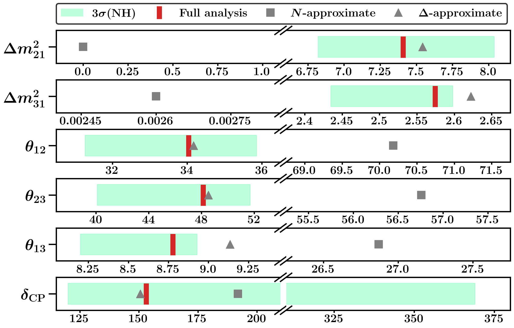
(a)

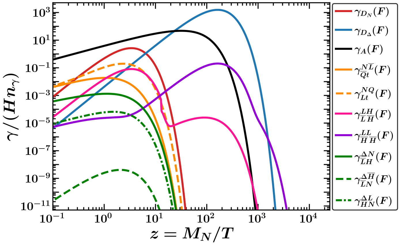
(b)

Figure 10: BP1: Left panel (10(a)) denotes the relative contribution of $N$ and $\Delta$ via type I and II seesaw mechanisms respectively with $3\sigma$ allowed oscillation parameters Esteban:2020cvm for normal hierarchy (NH). The red vertical line gives the values of the oscillation parameters for the full analysis whereas the gray square and triangle are the values obtained by only taking into the contribution of type I and type II seesaw respectively. Right panel (10(b)) shows the reaction densities (scaled by the product of Hubble parameter and photon number density) for different processes involved in the hybrid seesaw scenario with respect to $z=M_{N}/T$ which are calculated in full analysis denoted by $(F)$.

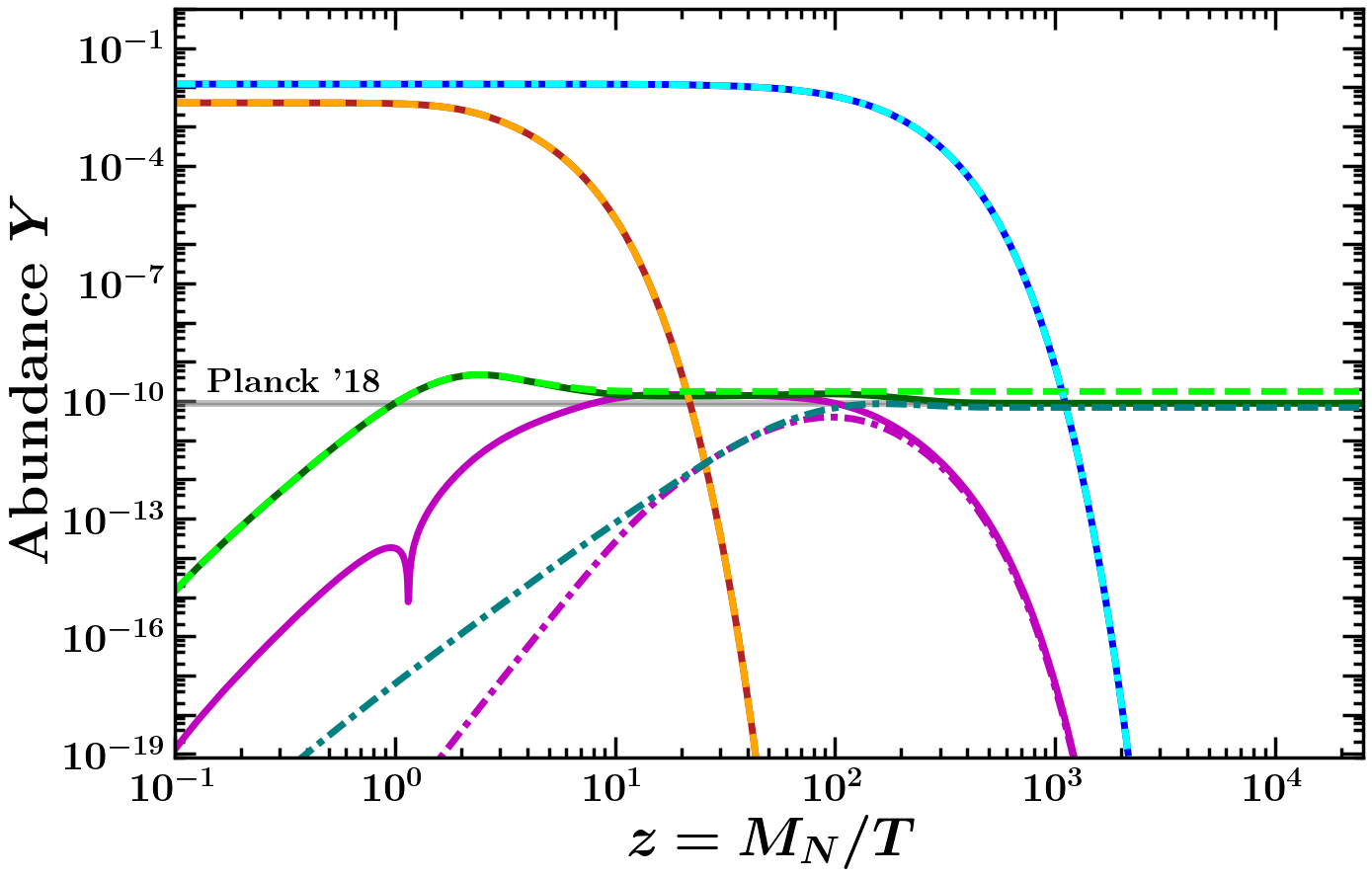
(a)

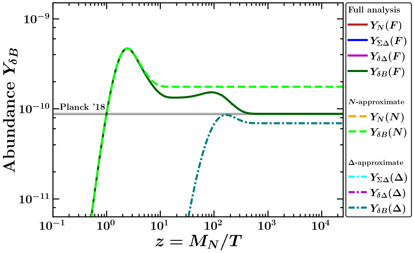
(b)

Figure 11: BP1: Left panel (11(a)) demonstrates the evolution of various abundances for the scenario of full analysis, $N$-approximate and $\Delta$-approximate indicated by solid, dashed and dot dashed lines and denoted by $F,N$ and $\Delta$ in the parentheses respectively. Right panel (11(b)) shows only the evolution of the baryon asymmetry for these three scenarios.

In the case of the first benchmark point BP1 given in table 1, the triplet contribution to the neutrino mass is dominant over the RHN, however the $\Delta m_{13}^{2}$ and $\theta_{13}$ satisfies the $3\sigma$ allowed ranges for normal hierarchy (NH) only when both the type I and II contributions are taken into account as shown in figure 10(a). The reaction densities for all the processes calculated in the full analysis denoted by $(F)$ are shown in figure 10(b). The evolution of various abundances are plotted against $z=M_{N}/T$ in figure 11(a) for the full analysis, $N$-approximate and $\Delta$-approximate analysis scenarios denoted by solid $(F)$, dashed $(N)$ and dotted $(\Delta)$ lines respectively. The abundances of RHN $(Y_{N})$ and triplet $(Y_{\Sigma\Delta})$ in the $N$-approximate and $\Delta$-approximate case respectively follows the full analysis whereas the abundance of asymmetric component of the triplet $Y_{\delta\Delta}$ in the $\Delta$-approximate scenario differs significantly from the full analysis. Owing to higher initial value of $\epsilon_{N}$ the baryon asymmetry calculated in the full analysis initially follow the $N$-approximate result and starts deviating around $z\sim 5$. Interestingly the asymmetry shows a peak like behavior at $z\sim 100$ as the triplet goes on-shell in the $LL\rightarrow\overline{H}\,\overline{H}$ process. The baryon asymmetry calculated in the full analysis starts to saturate around $z\sim 500$ and matches with the observed value measured by Planck Planck:2018vyg . As indicated in figure 11(b) the $N$-approximate ($\Delta$-approximate) scenario exhibit a deviation of the order of $\sim 100\,(20)\%$ from the full analysis.

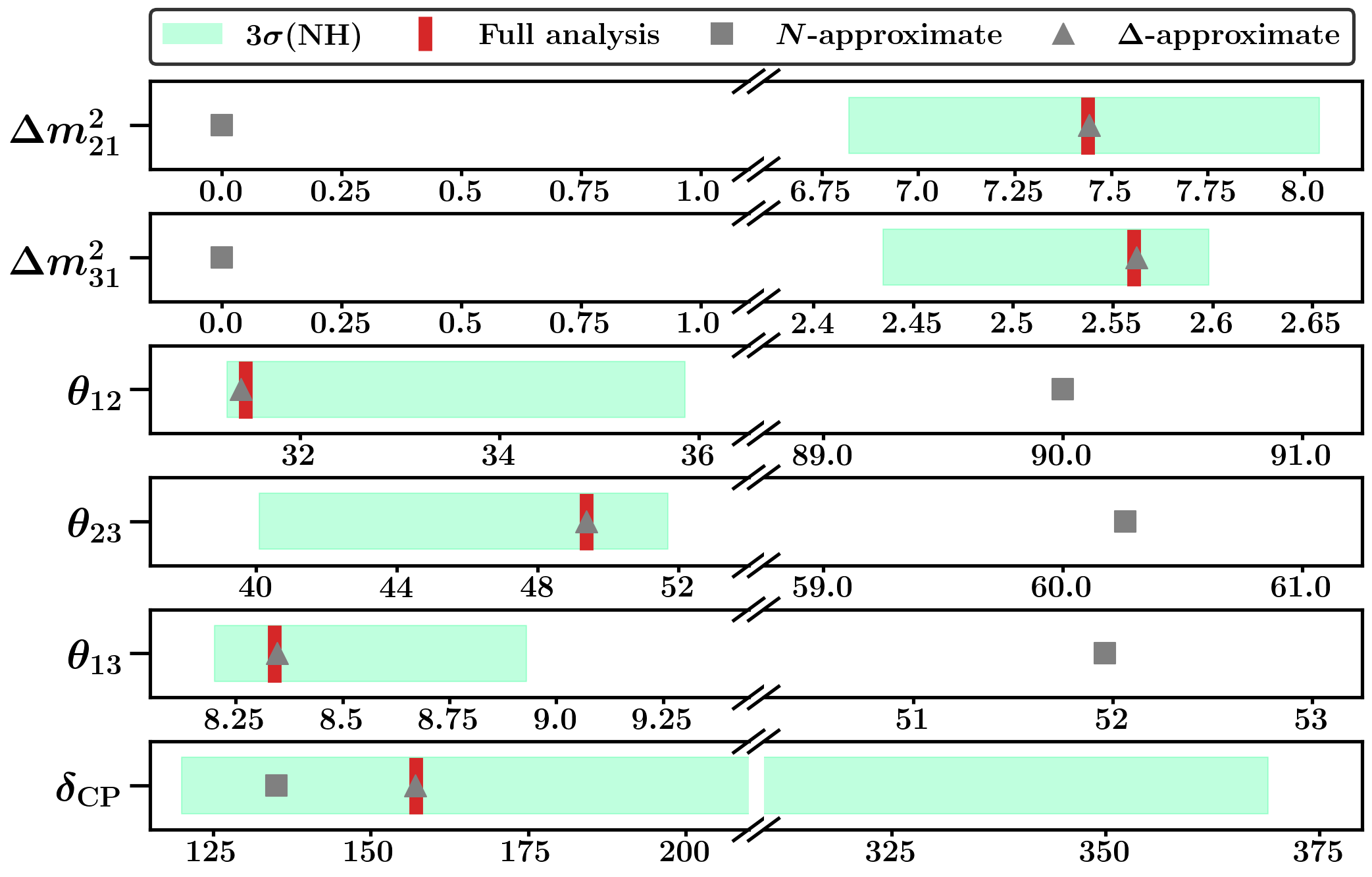
(a)

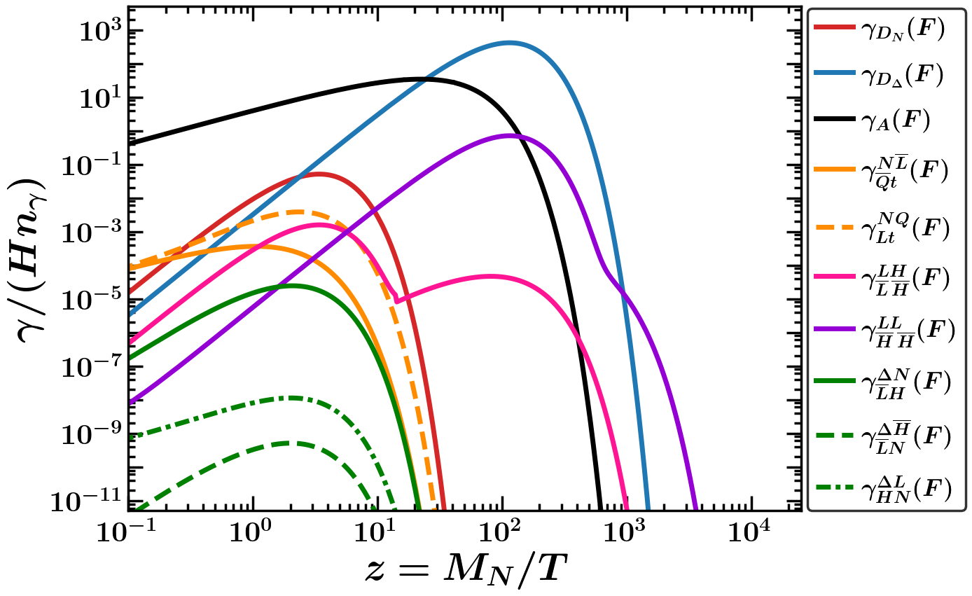
(b)

Figure 12: BP2: Same as of figure 10.

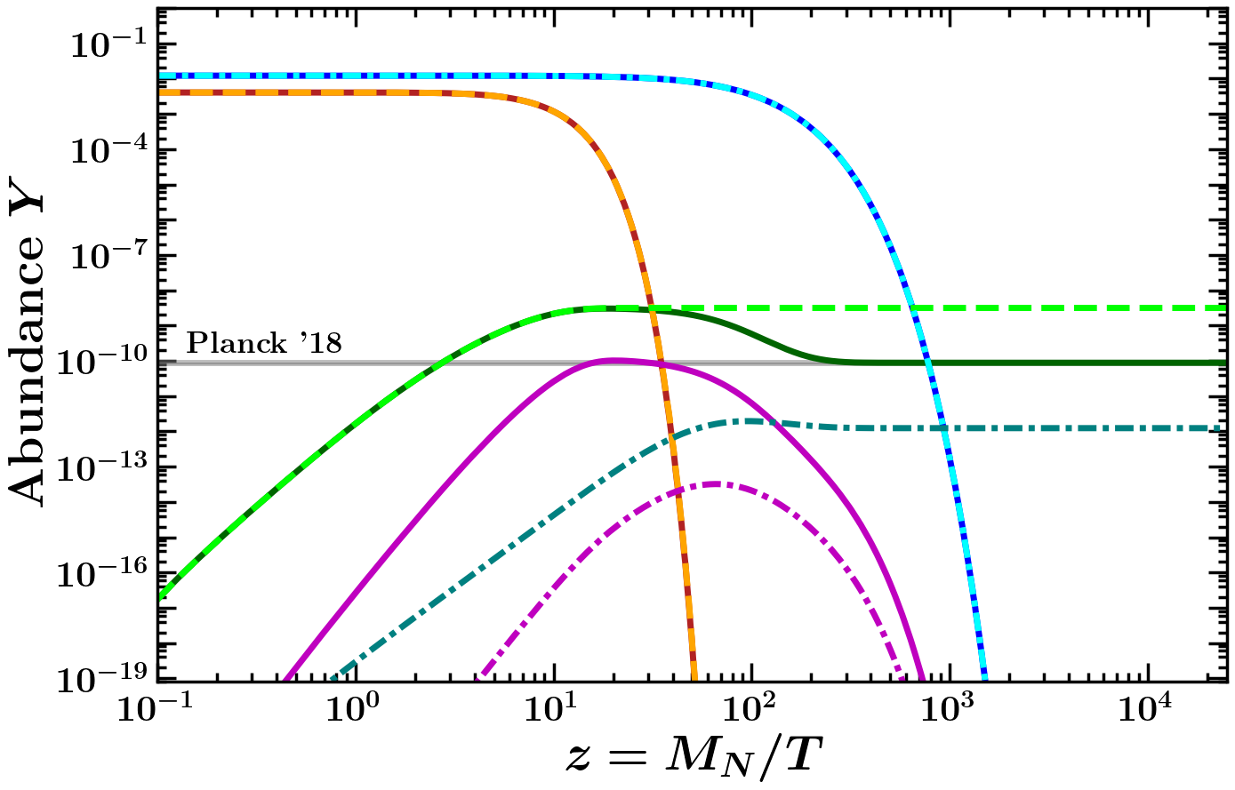
(a)

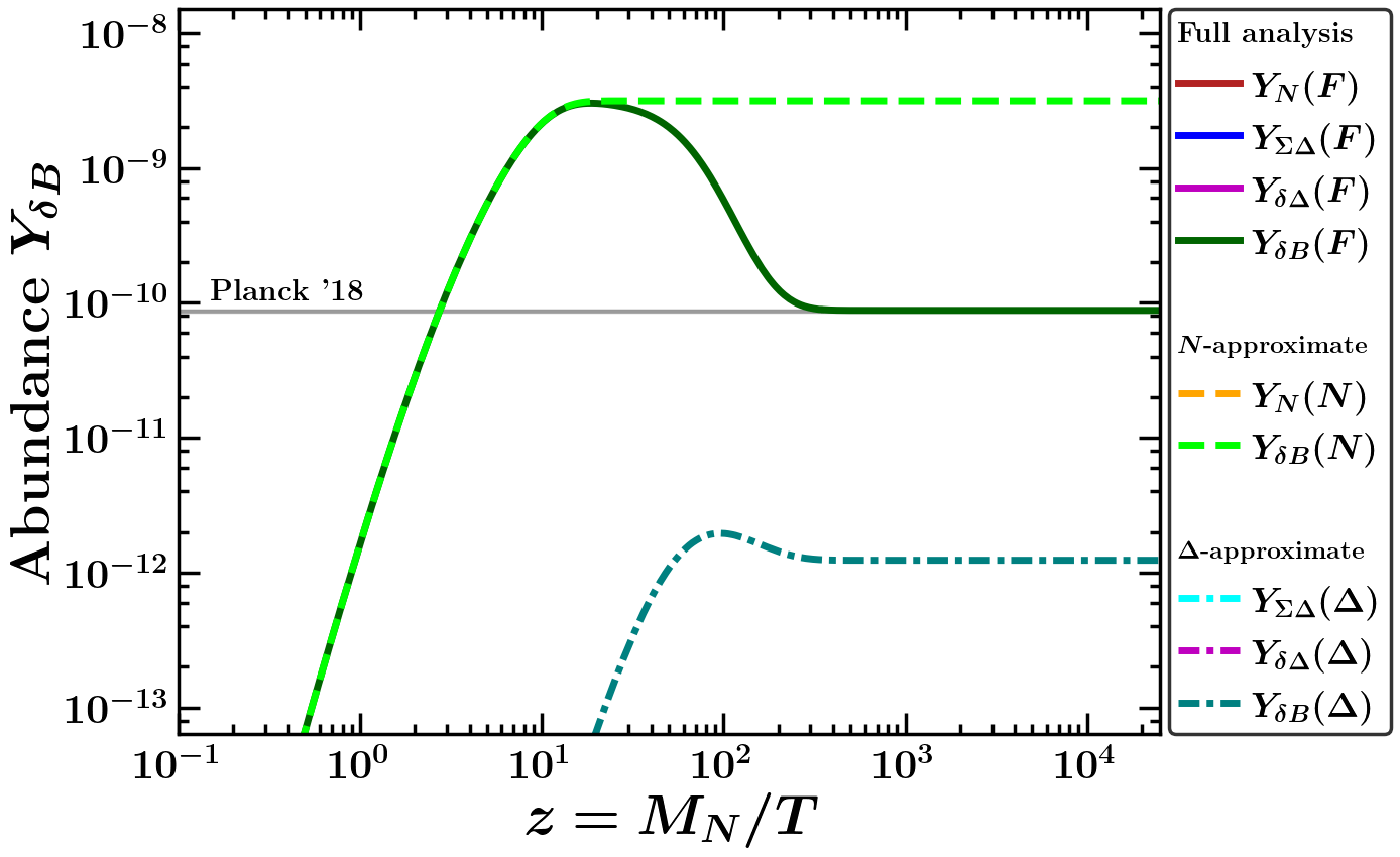
(b)

Figure 13: BP2: Same as of figure 11.

Similar situation for the nature of the baryon asymmetry can also be observed in the second benchmark point BP2, although all the oscillation parameters are solely determined by the type II contribution only as can be read off from figure 12(a). Due to a high value of $\epsilon_{r}$, the baryon asymmetry is controlled initially by the RHN upto $z\sim 10$ as can be seen from figure 13(b). However, there is roughly $\mathcal{O}(10^{2})$ deviation of the final baryon asymmetry to what have been obtained in each of the approximated scenarios.

These two representative benchmark points indicate that in spite of the lower scalar triplet mass the baryon asymmetry is not well estimated by the $\Delta$-approximate scenario. This is indicative of the phenomena that with relatively close mass scales the underlying mixed processes plays a significant role in determining the final baryon asymmetry and thus a full analysis keeping all mixed processes and $\Delta L=2$ processes revealing the full synergy of the two seesaws is crucial for an accurate determination of the baryon asymmetry in hybrid scenarios.

5 Validity of approximate analysis in hybrid leptogenesis

We present a quantitative analysis for the region of validity of the approximate analysis of leptogenesis with hierarchical hybrid scenarios. We consider a representative RHN mass as $M_{N}=9.714\times 10^{3}$ GeV and fix the Yukawa couplings at $\mathcal{Y}_{\nu}\sim\mathcal{O}(10^{-2})$ and $\mathcal{Y}_{\Delta}\sim\mathcal{O}(10^{-3})$. The exact values chosen are given in table 2 for completeness. The trilinear coupling to triplet mass ratio is also kept unchanged at $\mu/M_{\Delta}=0.038$ and the ratio of CP asymmetry parameter is $\epsilon_{r}=1.227$.

$\mathcal{Y}_{\nu}/10^{-2}$	$\mathcal{Y}_{\Delta}/10^{-3}$
$\begin{pmatrix}2.456+i\ 7.704\\ 5.437+i\ 0.788\\ 2.788+i\ 1.440\end{pmatrix}$	$\begin{pmatrix}5.708&2.846+i\ 5.774&9.976+i\ 2.802\\ \cdot&41.990&36.830+i\ 10.025\\ \cdot&\cdot&29.244\end{pmatrix}$

Table 2: Yukawa couplings of RHN and the scalar triplet

We define a degeneracy parameter $\mathcal{D}$ given by

$$\mathcal{D}\equiv\dfrac{r-1}{r+1}=\dfrac{M_{\Delta}-M_{N}}{M_{\Delta}+M_{N}}$$ (13)

which ranges between $[-1,\ 1]$ and gives an estimate of the mass degeneracy in the hybrid leptogenesis scenario and the error with respect to the full analysis is defined as

$$\zeta=\dfrac{Y_{\delta B}^{0}-Y_{\delta B}^{0}(F)}{Y_{\delta B}^{0}(F)}\ .$$ (14)

The final value of the baryon asymmetry is calculated in the full calculation and in approximated scenarios and plotted against the degeneracy parameter shown in figure 14(a) and the relative error of $N/\Delta$-approximate calculations with respect to the full analysis is shown in figure 14(b).

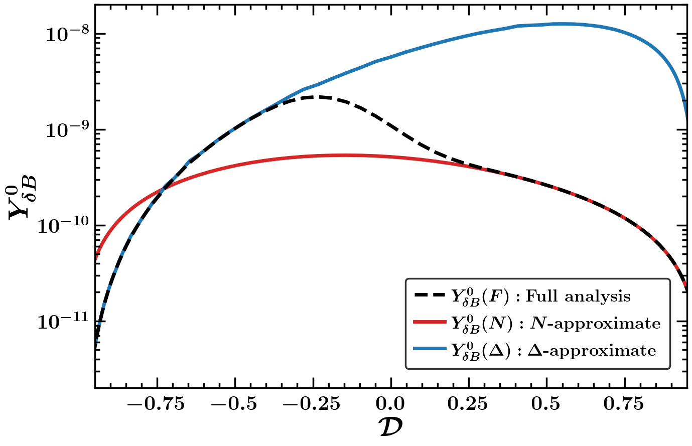
(a)

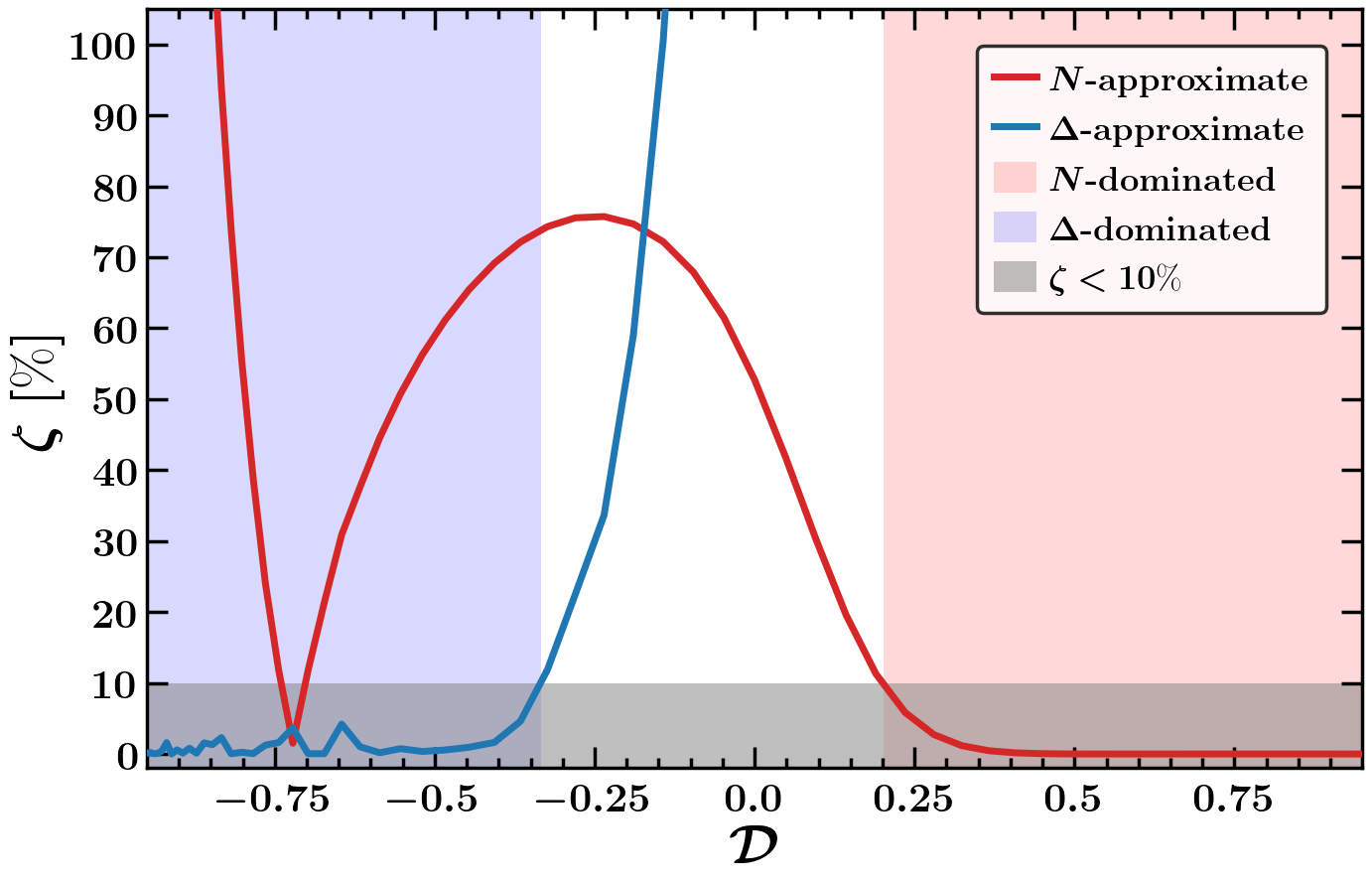
(b)

Figure 14: Left panel shows the final value of baryon asymmetry in the full analysis, $N$-approximate and $\Delta$-approximate scenarios denoted by black dashed, solid red and solid blue lines respectively. Right panel denotes the error which one obtains in the $N(\Delta)$-approximate calculations in comparison with the full analysis denoted by blue (red) solid curves. The red (blue) shaded region denotes that the $N(\Delta)$-approximate calculations are in well approximations of the full analysis with an error of less than $10\%$ denoted by the gray shaded region.

The lightest of the decaying particle usually dictates the fate of the final baryon asymmetry in the case of hierarchical spectrum with comparable values of CP asymmetry parameters. As can be clearly seen in figure 14(a) for large degeneracy with $\mathcal{D}\gtrsim|0.25|$ the full analysis represented by the black dashed line agrees with the $\Delta(N)$-approximate results represented by the blue (red) solid lines. More quantitatively this region maps to the blue (red) shaded region in figure 14(b) where the $\Delta(N)$-approximate analysis is within $10\%$ of the results obtained with the full calculation.

The mixed topology processes become numerically significant and the approximate results starts deviating from the complete analysis modulo local numerical artifacts arising due to fine tuned cancellations. Given the competing errors from thermal corrections Giudice:2003jh at $10\%$ we can consider $\mathcal{D}\gtrsim|0.25|$ as the limit for the validity of the approximated results beyond which a more careful complete analysis including all mixed processes is warranted. In case of hierarchical primordial CP asymmetries $\epsilon_{r}\sim\epsilon_{N}/\epsilon_{\Delta}$ the region of validity of the approximate solution shrinks further making the usage of the complete analysis more imperative.

It is well known that the lightest of the heavy particles dictates the fate of the final baryon asymmetry in the case of hierarchical mass spectrum and comparable values of CP asymmetry parameters. At lower (higher) values of $d$ the triplet (RHN) approximated results denoted by blue (red) solid line matches with the full analysis denoted by the black dashed line as can be seen in figure 14(a). This region i.e $d\gtrsim|0.25|$ is indicated by red (blue) shade where the considering only the lightest heavy particle i.e RHN (triplet) in the BEs of leptogenesis yields less than $10\%$ error. However, as the heavy particles become degenerate i.e $d\sim 0$, both the approximated analysis results in more than $50\%$ error around $d\sim 0$ as shown in figure 14(b). It is also important to notice that due to the interference of various Feynman diagrams there can be accidental cancellations in the full analysis which results in low error values for the approximated solutions resulting a dip in the error at any specific value of $r$ which is not known a priori. However, the error grows rapidly if one starts to go away from the dip which can only happen due to the artifact of interferences in hybrid processes.

In this benchmark point we find that if the CP asymmetries produced by heavy particles are comparable then taking into account both of these particles in the full calculation yields is necessary when the degeneracy parameter is less than $\sim 0.2$. However, in the presence of hierarchical values of CP asymmetry parameters one needs to consider the full analysis for even larger range of degeneracy parameter.

6 Conclusion

It is conceivable that under various circumstances, more than one seesaw framework is operative, simultaneously contributing to the neutrino mass parameters and driving baryogenesis through leptogenesis. The conventional approach has been to consider leptogenesis being dominated by the lightest species with the understanding that the asymmetry created at a higher scale is expected to be washed out due to the dynamics of the lighter degrees of freedom. It has been pointed out previously that this assumption gets modified when the initial asymmetry created by the CP violating decays of the heavy state(s) is substantial such that it may still account for the present-day matter-antimatter asymmetry due to incomplete washout.

In this work we point out a complementary scenario in a hybrid seesaw framework where the interplay of both the heavier and lighter species remains important. As the mass scales approach each other, certain (often neglected) scattering processes involving both the states become numerically significant. Even with moderate hierarchy of scales, these mixed topology processes require a complete tracing of the asymmetry keeping all the species in play. The final asymmetry in this case can significantly differ from the usual approximated estimates obtained by assuming leptogenesis being dominated by the lightest seesaw state.

We demonstrate the impact of such mixed processes for a hybrid type I + II leptogenesis framework. We show that for certain regions of the parameter space the complete analysis including these novel processes can result in more than $100\%$ correction in the final asymmetry as compared to the approximated results obtained assuming leptogenesis being dominated by the lightest species. The region of validity of the approximate result crucially depends on the extent of degeneracy between the two seesaw scales. While we demonstrate the importance of the complete analysis with the inclusion of the mixed topology scattering processes within the context of a specific scenario, the implications are more general and would be applicable to any hybrid leptogenesis framework.

Appendix A Notation and conventions utilised in the Boltzmann equations

The evolution of the number density $n_{X}$ for a species $X$ is conventionally described by the Boltzmann transport equation given by,

$$\dfrac{dY_{X}}{dz} =-\dfrac{1}{zs(z)H(z)}{{\sum}}_{i_{j},f_{k}}\left[\dfrac{Y_{X}}{Y_{X}^{\text{eq}}}\cdot\prod_{j=1}^{m}\dfrac{Y_{i_{j}}}{Y_{i_{j}}^{\text{eq}}}\cdot\gamma\left(X+\sum_{j=1}^{m}i_{j}\longrightarrow\sum_{k=1}^{n}f_{k}\right)\right.$$

$$\hskip 118.07875pt-\left.\prod_{k=1}^{n}\dfrac{Y_{f_{k}}}{Y_{f_{k}}^{\text{eq}}}\cdot\gamma\left(\sum_{k=1}^{n}f_{k}\longrightarrow X+\sum_{j=1}^{m}i_{j}\right)\right]\ ,$$ (A-1)

where $Y_{X}=n_{X}/s$ is the comoving number density and $z=M_{N}/T$. The Hubble parameter $H(z)$ and the entropy density $s(z)$ is given by

$$H(z)=\sqrt{\dfrac{8g_{*}}{\pi}}\dfrac{M_{N}^{2}}{M_{\text{Pl}}}\dfrac{1}{z^{2}}\ ;\quad s(z)=\dfrac{2\pi^{2}}{45}g_{*}\left(\dfrac{M_{N}}{z}\right)^{2}\ ,$$ (A-2)

where we calculate the effective degrees of freedom in the thermal bath is given by $g_{*}=114.5$ and the Planck mass is set at $M_{\text{Pl}}=1.22\times 10^{19}$ GeV. The equilibrium number density of RHN, triplet and SM (lepton and Higgs) doublets appearing in eq. 9 are respectively given by

$$n_{N}^{\text{eq}}=\dfrac{1}{\pi^{2}}M_{N}^{3}\dfrac{K_{2}(z)}{z};\quad n_{\Sigma\Delta}^{\text{eq}}=\dfrac{3r^{2}}{\pi^{2}}M_{\Delta}^{3}\dfrac{K_{2}(rz)}{z};\quad n_{L/H}^{\text{eq}}=\dfrac{2}{\pi^{2}}\left(\dfrac{M_{N}}{z}\right)^{3}\ ,$$ (A-3)

where $r$ is the mass ratio of triplet to the RHN defined above as $r=M_{\Delta}/M_{N}$ throughout the text.

Appendix B Calculation of reaction densities

In this section we provide a systematic calculation of all the reaction densities used in this work. The reaction density of any generic process $X+i_{1}+i_{2}+i_{3}+\cdots i_{m}\longrightarrow f_{1}+f_{2}+f_{3}+\cdots f_{n}$ is given by

$$\gamma^{X\,i_{1}\,i_{2}\,i_{3}\,\cdots i_{m}}_{f_{1}\,f_{2}\,f_{3}\,\cdots f_{n}} \equiv\gamma\left(X+\sum_{j=1}^{m}i_{j}\rightarrow\sum_{k=1}^{n}f_{k}\right)$$

$$=\int\dfrac{d^{3}p_{X}}{(2\pi)^{3}\,2E_{X}}f_{X}(E_{X})\prod_{j=1}^{m}\dfrac{d^{3}p_{i_{j}}}{(2\pi)^{3}\,2E_{i_{j}}}f_{i_{j}}(E_{i_{j}})\prod_{k=1}^{n}\dfrac{d^{3}p_{f_{k}}}{(2\pi)^{3}\,2E_{f_{k}}}\Big{[}1\pm f_{f_{k}}(E_{f_{k}})\Big{]}$$

$$\times(2\pi)^{4}\delta\left(p_{X}+\sum_{j=1}^{m}p_{i_{j}}-\sum_{k=1}^{n}p_{f_{k}}\right)\times\left|\mathcal{M}\left(X+\sum_{j=1}^{m}i_{j}\rightarrow\sum_{k=1}^{n}f_{k}\right)\right|^{2}\ ,$$ (B-4)

where $f_{p}(E_{p})\sim e^{-E_{p}/T}$ is the distribution function of any particle $p$ as a function of the its energy $(E_{p})$ and $|\mathcal{M}|^{2}$ is the squared transition amplitude of that specific process. The positive or negative sign in the factor $\big{[}1\pm f_{f_{k}}(E_{f_{k}})\big{]}$ depends on whether the $k$-th final state is a boson or a fermion, however, in the dilute gas approximation one can approximate the factor to unity. We also use Maxwell-Boltzmann distribution function for the initial state particles for various processes.

For $1\rightarrow 2$ decay the general formula given in eq. B simplifies to Davidson:2008bu

$$\gamma^{X}_{f_{1}\,f_{2}}=n_{X}^{\text{eq}}\dfrac{K_{1}(z)}{K_{2}(z)}\Gamma_{X}\ ,$$ (B-5)

where $\Gamma_{X}$ is the decay width of $X$ in the rest frame.

For a generic $2\rightarrow 2$ scattering process the reaction densities in the c.o.m frame is given by Giudice:2003jh ; Davidson:2008bu

$$\gamma^{1\,2}_{3\,4}\equiv\gamma(1\,2\rightarrow 3\,4)=\dfrac{T}{64\pi^{4}}\int_{s_{\text{min}}}^{\infty}ds\,\sqrt{s}\,K_{1}(z\sqrt{s})\,\widehat{\sigma}(s)\ ,$$ (B-6)

with $s_{\text{min}}=\text{Max}\left[\,(m_{1}+m_{2})^{2},(m_{3}+m_{4})^{2}\,\right]$ and the reduced cross section $\widehat{\sigma}$ given by Luty:1992un

$$\widehat{\sigma}(s)=\dfrac{1}{8\pi s}\int_{t_{-}}^{t_{+}}\big{|}\mathcal{M}_{1\,2\rightarrow 3\,4}\,(s,t)\big{|}^{2}\ dt\ ,$$ (B-7)

where $t$ is the Mandelstam variable with the limits ParticleDataGroup:2022pth

$$t_{\pm}=\dfrac{1}{4s}\left[\left(m_{1}^{2}-m_{2}^{2}-m_{3}^{2}+m_{4}^{2}\right)^{2}-\left\{\lambda^{1/2}\left(s,m_{1}^{2},m_{2}^{2}\right)\mp\lambda^{1/2}\left(s,m_{3}^{2},m_{4}^{2}\right)\right\}^{2}\right]\ .$$ (B-8)

For a s-channel process this can be expressed in the closed form by

$$\widehat{\sigma}(s)=\dfrac{1}{8\pi}\lambda^{1/2}(1,m_{1}^{2}/s,m_{2}^{2}/s)\ \lambda^{1/2}(1,m_{1}^{2}/s,m_{2}^{2}/s)\ \big{|}\mathcal{M}_{1\,2\rightarrow 3\,4}\big{|}^{2}\ ,$$ (B-9)

where $\lambda$ is the Kallen function defined as $\lambda(a,b,c)\equiv a^{2}+b^{2}+c^{2}-2ab-2bc-2ca$.

It is evident from eq. B-6 and eq. B-9 that the reduced cross section is dimensionless and thus it is more convenient to express several expressions in terms of dimensionless quantities defined as

$$x=\dfrac{s}{M_{N}^{2}}\ ;\ y=\dfrac{t}{M_{N}^{2}}\ ;\ y_{\pm}=\dfrac{t_{\pm}}{M_{N}^{2}}\ ;\ r=\dfrac{M_{\Delta}}{M_{N}}\ ;\ a_{i}=\dfrac{m_{i}^{2}}{M_{N}^{2}}\ ,\ a_{\Gamma_{i}}=\dfrac{m_{i}^{2}}{M_{N}^{2}}\ \forall\ i\in[L,H]\ ,$$ (B-10)

where $a_{H}$ and $a_{L}$ are set to be $10^{-5}$ and $10^{-8}$ respectively Luty:1992un ; Hahn-Woernle:2009jyb to handle the infrared divergences. Using these dimensionless quantities the reaction density given in eq. B-6 and reduced cross section given in eq. B-7 can be respectively written as

$$\gamma^{1\,2}_{3\,4}=\dfrac{M_{N}^{4}}{64\pi^{4}z}\int_{x_{\text{min}}}^{\infty}dx\,\sqrt{x}\,K_{1}(z\sqrt{x})\,\widehat{\sigma}(x)\ ;\quad\widehat{\sigma}(x)=\dfrac{1}{8\pi x}\int_{y_{-}}^{y_{+}}\big{|}\mathcal{M}_{1\,2\rightarrow 3\,4}\,(y)\big{|}^{2}\ dy$$ (B-11)

where $x_{\text{min}}=s_{\text{min}}/M_{N}^{2}$. With these notations we list down the reduced cross section of all the various processes that are important for our analysis in the following subsections.

B.1 Standard processes within type I/II leptogenesis

The $\Delta L=1$ processes that are present in the pure type I seesaw are shown in figure 4 which involves the top quark and its Yukawa coupling with the Higgs denoted by $y_{t}=\sqrt{2}m_{t}/v_{H}$.

$\bullet$ Process: $N\,(p_{1})+L\,(p_{2})\rightarrow\overline{Q}\,(p_{3})+t_{R}\,(p_{4})$

$$x_{\text{min}} \simeq 1\ ,$$ (B-12)

$$\left|\mathcal{M}\right|^{2}(x) \simeq 3\cdot 2\,\text{Tr}\left({\mathcal{Y}_{N}}^{\dagger}\mathcal{Y}_{N}\right)y_{t}^{2}\,\left(\dfrac{x-1}{x}\right)^{2}\ ,$$

$$\widehat{\sigma}(x) =\dfrac{3}{4\pi}\text{Tr}\left({\mathcal{Y}_{N}}^{\dagger}\mathcal{Y}_{N}\right)y_{t}^{2}\left(\dfrac{x-1}{x}\right)^{2}\ .$$

$\bullet$ Process: $N\,(p_{1})+\overline{Q}\,(p_{2})\rightarrow L\,(p_{3})+t_{R}\,(p_{4})$ and $N\,(p_{1})+t_{R}\,(p_{2})\rightarrow L\,(p_{3})+\overline{Q}\,(p_{4})$

$$x_{\text{min}} \simeq 1\ ,$$ (B-13)

$$y_{-} \simeq 1-x\text{ and }y_{+}\simeq 0\ ,$$

$$\left|\mathcal{M}\right|^{2}(y) \simeq 3\cdot 2\,\text{Tr}\left({\mathcal{Y}_{N}}^{\dagger}\mathcal{Y}_{N}\right)y_{t}^{2}\,\dfrac{y(y-1)}{(y-a_{H})^{2}}\ ,$$

$$\widehat{\sigma}(x) =\dfrac{3}{4\pi}\text{Tr}\left({\mathcal{Y}_{N}}^{\dagger}\mathcal{Y}_{N}\right)y_{t}^{2}\left(\dfrac{x-1}{x}\right)\left\{\dfrac{x-2+2a_{H}}{x-1+a_{H}}+\dfrac{1-2a_{H}}{x-1}\,\text{ln}\left(\dfrac{x-1+a_{H}}{a_{H}}\right)\right\}\ .$$

The reduced cross section for gauge induced triplet scattering processes in type II seesaw framework are given as Sierra:2014tqa

$$x_{\text{min}} \simeq 4r^{2}\ ,$$ (B-14)

$$\widehat{\sigma}(x) =\dfrac{1}{36\pi}\bigg{[}(5C_{2}-11C_{1})w^{3}+3(w^{2}-1)\left\{2C_{1}+C_{2}(w^{2}-1)\right\}\,\text{ln}\left(\dfrac{1+w}{1-w}\right)$$

$$\hskip 32.72049pt+\,(15C_{1}-3C_{2})w\bigg{]}+\left(\dfrac{41g_{1}^{4}+50g_{2}^{4}}{48\pi}\right)r^{3/2}$$

$$\text{with }C_{1}=3g_{1}^{4}+12g_{1}^{2}g_{2}^{2}+12g_{2}^{4}\ ;\ C_{2}=3g_{1}^{4}+12g_{1}^{2}g_{2}^{2}+6g_{2}^{4}\ ;\ w=\sqrt{1-\dfrac{4r^{2}}{x}}\ ,$$

where $g_{1}$ and $g_{2}$ are the gauge couplings for $U(1)$ and $SU(2)_{L}$ gauge groups respectively.

B.2 New hybrid processes

Within the hybrid framework there are three mixed scattering processes where both $N$ and $\Delta$ appear in the external legs. A discussion about their reduced cross sections are now in order.

$\bullet$ Process: $\Delta\,(p_{1})+N\,(p_{2})\rightarrow\overline{L}\,(p_{3})+H\,(p_{4})$

As shown in figure 5 that consists of two Feynman diagrams with amplitude denoted as $\mathcal{M}_{L}\,(\mathcal{M}_{H})$ for lepton (Higgs) mediated t-channel processes. The total squared amplitude and the reduced cross sections are given as

$$|\mathcal{M}|^{2}(y) =\left|i\mathcal{M}_{L}+i\mathcal{M}_{H}\right|^{2}=\left|\mathcal{M}_{L}\right|^{2}+\left(\mathcal{M}_{L}\mathcal{M}_{H}^{\dagger}+\mathcal{M}_{L}^{\dagger}\mathcal{M}_{H}\right)+\left|\mathcal{M}_{H}\right|^{2}\ ,$$ (B-15)

$$\widehat{\sigma}(x) =\int_{y_{-}}^{y^{+}}|\mathcal{M}|^{2}(y)dy=\widehat{\sigma}_{LL}(x)+\widehat{\sigma}_{LH}(x)+\widehat{\sigma}_{HH}(x)\ ,$$ (B-16)

where

$$x_{\text{min}} =\text{Max}\left[(r+1)^{2},(\sqrt{a_{L}}+\sqrt{a_{H}})^{2}\right]=(r+1)^{2}\ ,$$ (B-17)

$$y_{\pm} =\left[\left(r^{2}-1-a_{L}+a_{H}\right)^{2}-x^{2}\left\{\lambda^{1/2}\left(1,r^{2}/x,1/x\right)\mp\lambda^{1/2}\left(1,a_{L}^{2}/x,a_{H}^{2}/x\right)\right\}^{2}\right]\ ,$$ (B-18)

$$\widehat{\sigma}_{LL}(x) =\dfrac{\text{Tr}\left(\mathcal{Y}_{\Delta}\mathcal{Y}_{\nu}\mathcal{Y}_{\nu}^{\dagger}\mathcal{Y}_{\Delta}^{\dagger}\right)}{8\pi x}\left[(4a_{L}-x+1)\text{ln}|y-a_{L}|+\dfrac{(4a_{L}-r^{2})(-1+a_{H}-a_{L})}{y-a_{L}}\right]_{y_{-}}^{y_{+}}\ ,$$ (B-19)

$$\widehat{\sigma}_{LH}(x) =\dfrac{1}{8\pi x}\,2\mathfrak{Re}\left[\dfrac{\mu}{M_{N}}\text{Tr}\left(\mathcal{Y}_{\Delta}\mathcal{Y}_{\nu}\mathcal{Y}_{\nu}^{\dagger}\right)\right]\,\dfrac{1}{x-r^{2}-1}\ \times$$

$$\hskip 28.45274pt\Bigg{[}(4a_{L}-r^{2})\text{ln}|y-a_{L}|+(x-1-4a_{L})\text{ln}|y+x-r^{2}-1-a_{L}|\Bigg{]}_{y_{-}}^{y_{+}}\ ,$$ (B-20)

$$\widehat{\sigma}_{HH}(x) =\dfrac{1}{8\pi x}\,\left(\dfrac{\mu}{M_{N}}\right)^{2}\text{Tr}\left(\mathcal{Y}_{\nu}\mathcal{Y}_{\nu}^{\dagger}\right)\Bigg{[}\text{ln}|y+x-r^{2}-1-a_{L}|-\dfrac{1+a_{L}-a_{H}}{y+x-r^{2}-1-a_{L}}\Bigg{]}_{y_{-}}^{y_{+}}\ .$$ (B-21)

$\bullet$ Process: $\Delta\,(p_{1})+\overline{H}\,(p_{2})\rightarrow\overline{L}\,(p_{3})+N\,(p_{4})$

The process includes two Feynman diagrams, s-channel Higgs mediated diagram and t-channel lepton mediated diagram as shown in figure 6 with transition amplitudes denoted by $\mathcal{M}_{s}$ and $\mathcal{M}_{t}$ respectively. The total squared amplitude and reduced cross section can be written as

$$|\mathcal{M}|^{2}(y) =\left|i\mathcal{M}_{s}+i\mathcal{M}_{t}\right|^{2}=\left|\mathcal{M}_{s}\right|^{2}+\left(\mathcal{M}_{s}\mathcal{M}_{t}^{\dagger}+\mathcal{M}_{s}^{\dagger}\mathcal{M}_{t}\right)+\left|\mathcal{M}_{t}\right|^{2}\ ,$$ (B-22)

$$\widehat{\sigma}(x) =\int_{y_{-}}^{y^{+}}|\mathcal{M}|^{2}(y)dy=\widehat{\sigma}_{ss}(x)+\widehat{\sigma}_{st}(x)+\widehat{\sigma}_{tt}(x)\ ,$$ (B-23)

where

$$x_{\text{min}} =\text{Max}\left[(r+\sqrt{a_{H}})^{2},(\sqrt{a_{L}}+1)^{2}\right]\ ,$$ (B-24)

$$y_{\pm} =\left[\left(r^{2}-a_{H}-a_{L}+1\right)^{2}-x^{2}\left\{\lambda^{1/2}\left(1,r^{2}/x,a_{H}/x\right)\mp\lambda^{1/2}\left(1,a_{L}^{2}/x,1/x\right)\right\}^{2}\right]\ ,$$ (B-25)

$$\widehat{\sigma}_{ss}(x) =\dfrac{1}{8\pi}\,\left(\dfrac{\mu}{M_{N}}\right)^{2}\text{Tr}\left(\mathcal{Y}_{\nu}\mathcal{Y}_{\nu}^{\dagger}\right)\lambda^{1/2}\left(1,r^{2}/x,a_{H}/x\right)\,\lambda^{1/2}\left(1,a_{L}/x,1/x\right)\,\dfrac{x-1-a_{L}}{(x-a_{H})^{2}}\ ,$$ (B-26)

$$\widehat{\sigma}_{st}(x) =\dfrac{1}{8\pi x}\,2\mathfrak{Re}\left[\dfrac{\mu}{M_{N}}\text{Tr}\left(\mathcal{Y}_{\Delta}\mathcal{Y}_{\nu}\mathcal{Y}_{\nu}^{\dagger}\right)\right]\,\dfrac{1}{x-a_{H}}\Bigg{[}y+(4a_{L}-r^{2})\text{ln}|y-a_{L}|\Bigg{]}_{y_{-}}^{y_{+}}\ ,$$ (B-27)

$$\widehat{\sigma}_{tt}(x) =-\dfrac{\text{Tr}\left(\mathcal{Y}_{\Delta}\mathcal{Y}_{\nu}\mathcal{Y}_{\nu}^{\dagger}\mathcal{Y}_{\Delta}^{\dagger}\right)}{8\pi x}\,\Bigg{[}y+\dfrac{(r^{2}-4a_{L})(1+a_{L}-a_{H})}{y-a_{L}}$$

$$\hskip 113.81102pt+(x-a_{H}-r^{2}+4a_{L})\text{ln}|y-a_{L}|\Bigg{]}_{y_{-}}^{y_{+}}\ .$$ (B-28)

$\bullet$ Process: $\Delta\,(p_{1})+L\,(p_{2})\rightarrow H\,(p_{3})+N\,(p_{4})$

The process is depicted in figure 7 with two Feynman diagrams mediated by s-channel lepton (as shown in figure 7(a)) and t-channel Higgs (as shown in figure 7(b)) with amplitude $\mathcal{M}_{s}$ and $\mathcal{M}_{t}$ respectively. The corresponding expressions are given by,

$$x_{\text{min}} =\text{Max}\left[(r+\sqrt{a_{L}})^{2},(\sqrt{a_{H}}+1)^{2}\right]\ ,$$ (B-29)

$$y_{\pm} =\left[\left(r^{2}-a_{L}-a_{H}+1\right)^{2}-x^{2}\left\{\lambda^{1/2}\left(1,r^{2}/x,a_{L}/x\right)\mp\lambda^{1/2}\left(1,a_{H}^{2}/x,1/x\right)\right\}^{2}\right]\ ,$$ (B-30)

$$\widehat{\sigma}_{ss}(x) =\dfrac{\text{Tr}\left(\mathcal{Y}_{\Delta}\mathcal{Y}_{\nu}\mathcal{Y}_{\nu}^{\dagger}\mathcal{Y}_{\Delta}^{\dagger}\right)}{8\pi x}\,\dfrac{1}{2(x-a_{L})^{2}}\,\Bigg{[}y(x-r^{2}+3a_{L})\left(\dfrac{y}{2}+x-a_{L}-a_{H}\right)$$

$$\hskip 199.16928pt+y(r^{2}-4a_{L})(\dfrac{y}{2}-a_{L}-1)\Bigg{]}_{y_{-}}^{y_{+}}\ ,$$ (B-31)

$$\widehat{\sigma}_{st}(x) =\dfrac{1}{8\pi x}\,(-2)\mathfrak{Re}\left[\dfrac{\mu}{M_{N}}\text{Tr}\left(\mathcal{Y}_{\Delta}\mathcal{Y}_{\nu}\mathcal{Y}_{\nu}^{\mathsf{T}}\right)\right]\,\dfrac{x-r^{2}+3a_{L}}{x-a_{L}}\Bigg{[}\text{ln}|y-a_{H}|\Bigg{]}_{y_{-}}^{y_{+}}\ ,$$ (B-32)

$$\widehat{\sigma}_{tt}(x) =-\dfrac{1}{8\pi x}\,\left(\dfrac{\mu}{M_{N}}\right)^{2}\text{Tr}\left(\mathcal{Y}_{\nu}\mathcal{Y}_{\nu}^{\dagger}\right)\,\Bigg{[}\dfrac{1+a_{L}-a_{H}}{y-a_{H}}+\text{ln}|y-a_{H}|\Bigg{]}_{y_{-}}^{y_{+}}\ .$$ (B-33)

B.3 $\Delta L=2$ processes

There are two $\Delta L=2$ processes mediated by heavy RHN or the triplet. Each of these processes given in figure 8 and 9 consists of three Feynman diagrams in this hybrid scenario whereas the number of diagrams reduces if one considers vanilla seesaw frameworks. It is important to consider only the off-shell part of the heavy unstable propagators in order to avoid double counting Kolb:1979qa ; Giudice:2003jh ; Pilaftsis:2003gt ; Ala-Mattinen:2023rbm . We adopt the following conventions for the Breit-Wigner propagator,

$$P^{-1}(x,a,b)=\dfrac{1}{x-a+i\sqrt{b}}\ ;\quad\left|D^{-1}_{\text{sub}}(x,a,b)\right|^{2}=\left|P^{-1}(x,a,b)\right|^{2}-\dfrac{\pi}{\sqrt{b}}\delta(x-a)$$ (B-34)

where $\delta(x)$ is the Dirac delta function. The detailed expressions of the reduced cross section of these processes are given below.

$\bullet$ Process: $L\,(p_{1})+H\,(p_{2})\rightarrow L\,(p_{3})+H\,(p_{4})$

The process consists of three Feynman diagrams, RHN mediated s-channel (figure 8(a)) and u-channel (figure 8(b)) diagram and triplet mediated t-channel (8(c)) diagram for which the transition amplitude is denoted my $\mathcal{M}_{s}$, $\mathcal{M}_{u}$ and $\mathcal{M}_{t}$ respectively. The squared amplitude and the corresponding reduced cross section can be written as

$$|\mathcal{M}|^{2}(y) =|\mathcal{M}_{s}|^{2}+|\mathcal{M}_{u}|^{2}+|\mathcal{M}_{t}|^{2}$$

$$+\left(\mathcal{M}_{s}\mathcal{M}_{u}^{\dagger}+\mathcal{M}_{s}^{\dagger}\mathcal{M}_{u}\right)+\left(\mathcal{M}_{u}\mathcal{M}_{t}^{\dagger}+\mathcal{M}_{u}^{\dagger}\mathcal{M}_{t}\right)+\left(\mathcal{M}_{t}\mathcal{M}_{s}^{\dagger}+\mathcal{M}_{t}^{\dagger}\mathcal{M}_{s}\right)\ ,$$ (B-35)

$$\widehat{\sigma}(x) =\int_{y_{-}}^{y^{+}}|\mathcal{M}|^{2}(y)dy=\widehat{\sigma}_{ss}(x)+\widehat{\sigma}_{uu}(x)+\widehat{\sigma}_{tt}(x)+\widehat{\sigma}_{su}(x)+\widehat{\sigma}_{ut}(x)+\widehat{\sigma}_{ts}(x)\ ,$$ (B-36)

where the explicit expressions of various quantities are given below

$$x_{\text{min}} =(\sqrt{a_{L}}+\sqrt{a_{H}})^{2}\ ,$$ (B-37)

$$y_{-} =-x\lambda(1,a_{L}/x,a_{H}/x)\text{ and }y_{+}=0\ ,$$ (B-38)

$$\widehat{\sigma}_{ss}(x) =\dfrac{1}{8\pi x}\left(\text{Tr}\left(\mathcal{Y}_{\nu}\mathcal{Y}_{\nu}^{\dagger}\right)\right)^{2}\left|D^{-1}_{\text{sub}}(x,1,a_{\Gamma_{N}})\right|^{2}\Bigg{[}2a_{L}y-\dfrac{y^{2}}{2}\Bigg{]}_{y_{-}}^{y_{+}}\ ,$$ (B-39)

$$\widehat{\sigma}_{uu}(x) =\dfrac{1}{8\pi x}\left(\text{Tr}\left(\mathcal{Y}_{\nu}\mathcal{Y}_{\nu}^{\dagger}\right)\right)^{2}\Bigg{[}\dfrac{D}{\sqrt{a_{\Gamma_{N}}}}\tan^{-1}\dfrac{y+C}{\sqrt{a_{\Gamma_{N}}}}-\dfrac{1}{2}\text{ln}\left|(y+C)^{2}+a_{\Gamma_{N}}\right|\Bigg{]}_{y_{-}}^{y_{+}}\ ,$$ (B-40)

$$\widehat{\sigma}_{tt}(x) =-\dfrac{1}{8\pi x}\left(\dfrac{\mu}{M_{N}}\right)^{2}\text{Tr}\left(\mathcal{Y}_{\Delta}\mathcal{Y}_{\Delta}^{\dagger}\right)\ \times$$

$$\hskip 85.35826pt\Bigg{[}\dfrac{1}{2}\text{ln}\left|(y-r^{2})^{2}+r^{2}a_{\Gamma_{\Delta}}\right|+\dfrac{r^{2}-4a_{L}}{r\sqrt{a_{\Gamma_{\Delta}}}}\tan^{-1}\dfrac{y-r^{2}}{r\sqrt{a_{\Gamma_{\Delta}}}}\Bigg{]}_{y_{-}}^{y_{+}},$$ (B-41)

$$\widehat{\sigma}_{su}(x) =\dfrac{\left(\text{Tr}\left(\mathcal{Y}_{\nu}\mathcal{Y}_{\nu}^{\dagger}\right)\right)^{2}}{8\pi x}\dfrac{2(x-1)}{\left|P(x,1,a_{\Gamma_{N}})\right|^{2}}\ \times$$

$$\hskip 85.35826pt\Bigg{[}y-\sqrt{a_{\Gamma_{N}}}\tan^{-1}\dfrac{y+C}{\sqrt{a_{\Gamma_{N}}}}-\dfrac{D}{2}\text{ln}\left|(y+C)^{2}+a_{\Gamma_{N}}\right|\Bigg{]}_{y_{-}}^{y_{+}}\ ,$$ (B-42)

$$\widehat{\sigma}_{ut}(x) =\dfrac{1}{8\pi x}\,2\mathfrak{Re}\left\{\dfrac{\mu}{M_{N}}\text{Tr}\left(\mathcal{Y}_{\nu}\mathcal{Y}_{\nu}^{\mathsf{T}}\mathcal{Y}_{\Delta}\right)^{*}\Bigg{[}\dfrac{E+F}{F-G}\text{ln}|y+F|-\dfrac{E+G}{F-G}\text{ln}|y+G|\Bigg{]}_{y_{-}}^{y_{+}}\right\}\ ,$$ (B-43)

$$\widehat{\sigma}_{ts}(x) =-\dfrac{1}{8\pi x}\,2\mathfrak{Re}\left\{\text{Tr}\left(\mathcal{Y}_{\Delta}\mathcal{Y}_{\nu}\mathcal{Y}_{\nu}^{\mathsf{T}}\right)P^{-1}(x,1,a_{\Gamma_{N}})\Bigg{[}y+(-G^{*}-E)\text{ln}|y+G^{*}|\Bigg{]}_{y_{-}}^{y_{+}}\right\}\ ,$$ (B-44)

with

$$C =x+1-2a_{L}-2a_{H}\ ,$$ (B-45)

$$D =x+1-2a_{H}\ ,$$

$$E =4a_{L}\ ,$$

$$F =x+1-2a_{L}-2a_{H}-i\sqrt{a_{\Gamma_{N}}}\ ,$$

$$G =-r^{2}-ir\sqrt{a_{\Gamma_{\Delta}}}\ .$$

$\bullet$ Process: $L\,(p_{1})+L\,(p_{2})\rightarrow\overline{H}\,(p_{3})+\overline{H}\,(p_{4})$

The process consists of three Feynman diagrams, triplet mediated s-channel (figure 9(a)) and RHN mediated t-channel and u-channel (figure 9(b) and 9(c)) diagrams for which the transition amplitude is denoted my $\mathcal{M}_{s}$, $\mathcal{M}_{t}$ and $\mathcal{M}_{u}$ respectively. The squared amplitude and the corresponding reduced cross section can be written as

$$|\mathcal{M}|^{2}(y) =|\mathcal{M}_{s}|^{2}+|\mathcal{M}_{t}|^{2}+|\mathcal{M}_{u}|^{2}$$

$$+\left(\mathcal{M}_{s}\mathcal{M}_{t}^{\dagger}+\mathcal{M}_{s}^{\dagger}\mathcal{M}_{t}\right)+\left(\mathcal{M}_{t}\mathcal{M}_{u}^{\dagger}+\mathcal{M}_{t}^{\dagger}\mathcal{M}_{u}\right)+\left(\mathcal{M}_{u}\mathcal{M}_{s}^{\dagger}+\mathcal{M}_{u}^{\dagger}\mathcal{M}_{s}\right)\ ,$$ (B-46)

$$\widehat{\sigma}(x) =\int_{y_{-}}^{y^{+}}|\mathcal{M}|^{2}(y)dy=\widehat{\sigma}_{ss}(x)+\widehat{\sigma}_{tt}(x)+\widehat{\sigma}_{uu}(x)+\widehat{\sigma}_{st}(x)+\widehat{\sigma}_{tu}(x)+\widehat{\sigma}_{us}(x)\ ,$$ (B-47)

where the explicit expressions of various quantities are given below

$$x_{\text{min}} =4a_{H}\ ,$$ (B-48)

$$y_{\pm} =-\dfrac{x}{4}\left(\sqrt{1-\dfrac{4a_{L}}{x}}\mp\sqrt{1-\dfrac{4a_{H}}{x}}\right)^{2}\ ,$$ (B-49)

$$\widehat{\sigma}_{ss}(x) =\dfrac{1}{8\pi}\left(\dfrac{\mu}{M_{N}}\right)^{2}\text{Tr}\left(\mathcal{Y}_{\Delta}\mathcal{Y}_{\Delta}^{\dagger}\right)\sqrt{1-\dfrac{4a_{L}}{x}}\sqrt{1-\dfrac{4a_{H}}{x}}2(x-4a_{L})\left|D^{-1}_{\text{sub}}(x,r^{2},r^{2}a_{\Gamma_{\Delta}})\right|^{2}\ ,$$ (B-50)

$$\widehat{\sigma}_{tt}(x) =\dfrac{1}{8\pi x}\left(\text{Tr}\left(\mathcal{Y}_{\nu}\mathcal{Y}_{\nu}^{\dagger}\right)\right)^{2}\dfrac{x-2a_{L}}{\sqrt{a_{\Gamma_{N}}}}\Bigg{[}\tan^{-1}\dfrac{y-1}{\sqrt{a_{\Gamma_{N}}}}\Bigg{]}_{y_{-}}^{y_{+}}\ ,$$ (B-51)

$$\widehat{\sigma}_{uu}(x) =\dfrac{1}{8\pi x}\left(\text{Tr}\left(\mathcal{Y}_{\nu}\mathcal{Y}_{\nu}^{\dagger}\right)\right)^{2}\dfrac{x-2a_{L}}{\sqrt{a_{\Gamma_{N}}}}\Bigg{[}\tan^{-1}\dfrac{y+C}{\sqrt{a_{\Gamma_{N}}}}\Bigg{]}_{y_{-}}^{y_{+}}\ ,$$ (B-52)

$$\widehat{\sigma}_{st}(x) =\dfrac{1}{8\pi x}2\mathfrak{Re}\left\{\dfrac{\mu}{M_{N}}\text{Tr}\left(\mathcal{Y}_{\Delta}\mathcal{Y}_{\nu}^{*}\mathcal{Y}_{\nu}^{\dagger}\right)^{*}\dfrac{x-E}{x-H}\Bigg{[}\text{ln}|y+H|\Bigg{]}_{y_{-}}^{y_{+}}\right\}\ ,$$ (B-53)

$$\widehat{\sigma}_{tu}(x) =\dfrac{1}{8\pi x}2\mathfrak{Re}\left\{\left(\text{Tr}\left(\mathcal{Y}_{\nu}\mathcal{Y}_{\nu}^{\dagger}\right)\right)^{2}\dfrac{x-2a_{L}}{x+2(1-a_{L}-a_{H})}\Bigg{[}-\text{ln}|y+H^{*}|+\text{ln}|y+F^{*}|\Bigg{]}_{y_{-}}^{y_{+}}\right\}\ ,$$ (B-54)

$$\widehat{\sigma}_{us}(x) =\dfrac{1}{8\pi x}\,2\mathfrak{Re}\left\{\dfrac{\mu}{M_{N}}\text{Tr}\left(\mathcal{Y}_{\nu}\mathcal{Y}_{\nu}^{\mathsf{T}}\mathcal{Y}_{\Delta}^{\dagger}\right)\dfrac{x-E}{x+G}\Bigg{[}\text{ln}|y+G|\Bigg{]}_{y_{-}}^{y_{+}}\right\}\ ,$$ (B-55)

with $H=-1-i\sqrt{a_{\Gamma_{N}}}$ and other expressions same as given in eq. B-45.