∎
22email: mayala5@jhu.edu 33institutetext: Zein Sadek 44institutetext: Mechanical and Materials Engineering, Portland State University, Portland, OR 97201, USA 55institutetext: Ondřej Ferčák 66institutetext: Mechanical and Materials Engineering, Portland State University, Portland, OR 97201, USA 77institutetext: Raul Bayoán Cal 88institutetext: Mechanical and Materials Engineering, Portland State University, Portland, OR 97201, USA 99institutetext: Dennice F. Gayme 1010institutetext: Mechanical Engineering, Johns Hopkins University, Baltimore, MD 21218-2625, USA 1111institutetext: Charles Meneveau 1212institutetext: Mechanical Engineering, Johns Hopkins University, Baltimore, MD 21218-2625, USA
A Moving Surface Drag Model for LES of Wind over Waves
Abstract
Numerical prediction of the interactions between wind and ocean waves is essential for climate modeling and a wide range of offshore operations. Large Eddy Simulation (LES) of the marine atmospheric boundary layer is a practical numerical predictive tool but requires parameterization of surface fluxes at the air-water interface. Current momentum flux parameterizations primarily use wave-phase adapting computational grids, incurring high computational costs, or use an equilibrium model based on Monin-Obukhov similarity theory for rough surfaces that cannot resolve wave phase information. To include wave phase-resolving physics at a cost similar to the equilibrium model, the Moving Surface Drag (MOSD) model is introduced. It assumes ideal airflow over locally piece-wise planar representations of moving water wave surfaces. Horizontally unresolved interactions are still modeled using the equilibrium model. Validation against experimental and numerical datasets with known monochromatic waves demonstrates the robustness and accuracy of the model in representing wave-induced impacts on mean velocity and Reynolds stress profiles. The model is formulated to be applicable to a broad range of wave fields and its ability to represent cross-swell and multiple wavelength cases is illustrated. Additionally, the model is applied to LES of a laboratory-scale fixed-bottom offshore wind turbine model, and the results are compared with wind tunnel experimental data. The LES with the MOSD model shows good agreement in wind-wave-wake interactions and phase-dependent physics at a low computational cost. The model’s simplicity and minimal computational needs make it valuable for studying turbulent atmospheric-scale flows over the sea, particularly in offshore wind energy research.
Keywords:
Air-sea interaction Large eddy simulation Marine boundary layer Offshore wind energy1 Introduction
The interaction between wind and waves is a complicated multiscale process that occurs at the interface between the atmosphere and the ocean. Understanding the dynamics of wind-wave interactions is crucial not only for advancing our fundamental knowledge of the underlying physics, but also for practical applications such as weather forecasting, coastal engineering, and marine operations, such as offshore wind farm design and control. Extensive research has been devoted to investigating the wave-induced effects on the vertical structure of turbulent airflow above the ocean or wavy surfaces, with valuable insights gained from field measurements (Grachev and Fairall 2001; Donelan et al. 2006; Edson et al. 2007; Grare et al. 2018) and laboratory experiments (Snyder et al. 1981; Banner and Peirson 1998; Funke et al. 2021). These studies have facilitated the quantification of momentum transfer between the sea and the air medium. More recently, Buckley and Veron (2016), Buckley et al. (2020) and Yousefi et al. (2020) conducted meticulous particle image velocimetry (PIV) measurements of turbulent air above wind-generated waves, shedding light on the intricate airflow structure and wind stress above the wave surface. Their work quantified the impact of form (pressure) drag on the total air-water momentum flux, comparing it to the effects of viscous drag and its dependence on wave slope. Experimental studies by Peirson and Garcia (2008) and Grare et al. (2013) enabled the estimation of the wave growth rate and dissipation rate due to the energy transfer between wind and wave fields.
In recent years, numerical simulations have emerged as a vital tool for investigating the fundamental physics of turbulent flows. Early numerical models of turbulent flow over wavy surfaces (Gent and Taylor 1976; Al-Zanaidi and Hui 1984; Li et al. 2000) relied on Reynolds-averaged equations and eddy viscosity formulations, which yielded diverse predictions of wave growth due to the sensitivity of these quantities to the chosen turbulence closure scheme. Direct Numerical Simulations (DNS) have been employed as a much higher fidelity numerical approach to examine turbulent flows over complex geometries, such as wavy surfaces (Sullivan et al. 2000; Yang and Shen 2010; Deskos et al. 2022; Wu et al. 2022). While DNS has no need for parameterizations or subgrid-scale modeling, it is inherently limited to low or moderate Reynolds numbers due to the substantial computational costs associated with resolving viscous sublayer processes. In contrast to DNS, large eddy simulation (LES) offers the advantage of lower cost since the small scales of turbulence are modeled via a subgrid-scale model while still resolving the large-scale motions. Interactions between the atmospheric boundary layer (ABL) and waves have been extensively investigated using wall-resolved LES (WRLES), in which a no-slip boundary condition is applied to the wavy surface using sufficiently fine spatial resolution near the surface. Several WRLES studies study monochromatic waves (sinusoidal wave train) as the wavy boundary (Sullivan et al. 2008; Åkervik and Vartdal 2019; Zhang et al. 2019; Wang et al. 2021; Cao and Shen 2021; Hao et al. 2021), while others consider a complete ocean wave spectrum (Yang et al. 2014a; Hao and Shen 2019; Wang et al. 2020b). The viscous sublayer in the marine atmospheric boundary layer (MABL) is typically only fractions of millimeter thick. Therefore, WRLES is still limited to moderate Reynolds numbers, since its need to resolve near-wall structures makes its computational cost scaling not significantly lower than that of DNS (Yang and Griffin 2021). For both WRLES and DNS of turbulent flow over a waves, a boundary fitted grid or a terrain-following grid is typically employed to represent the surface in the numerical domain (Deskos et al. 2021), often called “wave-phase-resolved” approach. The use of this approach coupled with the high resolution near the wall enables an accurate resolution of phase-dependent wave effects and near-wall wave-induced turbulent effects. However, this comes at the expense of high and frequently prohibitive computational costs.
More cost-effective numerical simulations of wind fields can be accomplished using wall-modeled LES (WMLES), where the near-wall region must be modelled through wall models. Over the past decades a number of wall models have been developed for flow over on-shore rough terrain (Stoll et al. 2020), typically based on “Monin-Obukhov Similarity Theory” (MOST) (Moeng 1984) in geophysical applications or the logarithmic law in engineering applications (Piomelli and Balaras 2002). Within the MOST framework, the surface stress is determined by a surface roughness parameter () that incorporates the influence of unresolved surface features on the flow. However, the modeling of flow over moving surface waves has received less attention. The classical approach, known as the “wave-phase-averaged” approach, involves specifying an effective roughness length specifically for ocean waves. The Charnock model, introduced by Charnock (1955), is a widely adopted approach for parameterizing an equivalent effective roughness for ABLs over ocean waves. In recent years, several investigations have proposed other surface roughness relationships based on a wave-age and wave-steepness parametrization (Masuda and Kusaba 1987; Toba et al. 1990; Smith et al. 1992). However, all of the “wave-phase-averaged” approaches are highly dependent on empirical parameters, which must be tuned and can vary significantly from dataset to dataset (Deskos et al. 2022). Moreover, such methods cannot represent phase-dependent processes.
To address the current limitations of wind-wave interaction models, we aim to develop an approach that can resolve some phase-dependent wave effects while preserving the computational efficiency offered by phase-averaged approaches. Recently, Aiyer et al. (2023) have introduced a generalization of the horizontally resolved, vertically unresolved surface gradient model of Anderson and Meneveau (2010) that is based on momentum fluxes associated with the velocity differences between incoming wind and wave components. For applications to wave surfaces consisting of multiple wavelengths, the model by Aiyer et al. (2023) uses a superposition over the various constitutive wavenumbers of the imposed wave spectrum and introduces a wavelength-dependent drag coefficient. This prefactor can recover theoretical predictions of wave energy input rates at various wavelengths. With similar motivations, in this work we introduce a model that is not based on a superposition of forces over wave frequencies or wavelengths, but instead is based directly on knowledge of the local surface slope and its time evolution in physical space, without recourse to spectral descriptions and wavelength-dependent drag coefficients. The proposed Moving Surface Drag (MOSD) model relies on the assumption that windward facing portions of the wave are exposed to increased pressure distribution. This pressure field is modeled as that arising in ideal potential flow over an inclined plane (ramp flow), while the force from the pressure field on the back leeward side of the wave is neglected altogether based on the assumption of flow separation or near separation. Drag caused by horizontally unresolved scales (small-scale interactions) are still modeled using the traditional equilibrium wall model. The MOSD model enables us to represent phase-dependent effects of ocean waves in LES using a simple flat bottom surface boundary condition at a moderate computational cost that is of similar order of magnitude to that of the equilibrium wall model.
First, a detailed derivation and description of the MOSD model is provided in Sect. 2. In Sect. 3 the numerical code, numerical details and suite of test benchmark cases to be used for model validation are presented. The WMLES results are compared to the benchmark cases in Sect. 4. Furthermore, the general applicability of the MOSD model is illustrated for more general wave conditions and propagation directions in Sect. 5. To illustrate applicability of the model to offshore wind energy related problems, in Sect. 6 LES with the MOSD air-sea parameterization is undertaken to model the flow in a laboratory experiment of a fixed-bottom offshore wind turbine. WMLES data are compared with the laboratory experimental data. Finally, the main conclusions are summarized in Sect. 7.
2 Moving Surface Drag (MOSD) Model
The proposed MOving Surface Drag (MOSD) wall model is comprised of two components, a model based on ideal potential flow theory applied to windward facing portions of the surface to represent form drag caused by flow blockage due to the horizontally resolved features of moving waves, and an equilibrium wall stress that follows the local law-of-the-wall (or MOST) to model effects of entirely unresolved surface roughness features.
2.1 Windward Potential Flow Model
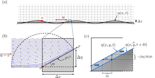
Lamb (1945) shows that an inviscid and irrotational assumption (ideal flow) can be applied to represent the dynamics of air flow over monochromatic waves of small amplitude. However, this representation results in the pressure distribution along the air-sea interface being out of phase with the gradient of the surface distribution, leading to zero average stress on the interface. Thus, no net form drag can be imparted onto the air in pure potential flow. Alternatively, in the proposed model we assume that potential flow only applies to the windward face of waves that are horizontally resolved in the LES and neglect any force coming from the leeward (downwind) portion of the surface by assuming the flow there to be separating or almost separating (the validity of this assumption will be discussed later on). In addition in each computational cell of length , the wave is represented locally as an inclined plane with inclination angle . The sketch shown in Fig.1 illustrates the basic idea. For reference, we use a Cartesian frame, with being the streamwise, vertical, and spanwise coordinates (also denoted as , and for the index notation). Moving with the local horizontal velocity of the wave surface , separately in each cell we assume that the flow arrives horizontally at a relative velocity (where is the horizontal air velocity at a vertical distance on the order of ). The flow is locally deflected upward at an angle . The flow is assumed to be ideal potential flow over an inclined plane (ramp flow). For such a flow, the streamfunction in cylindrical coordinates with origin at the lower point in the cell (where the flow is assumed to impinge against the surface) is given by:
| (1) |
where , is a constant, is the ramp angle and is the polar coordinate angle, as shown in Fig. 1.
On the inclined surface (which is purely radial) there is no tangential velocity normal to the surface ( = 0), and the parameter can be prescribed such that the radial velocity of the potential flow, at , equals far from the impingement point, i.e. when (small angles are assumed throughout). With this choice, the radial velocity becomes
| (2) |
Our aim is to obtain the total pressure force acting on the surface, whose horizontal projection represents the pressure drag due to the flow going over the ramp surface. We make the assumption of steady potential flow and thus apply a steady Bernoulli equation between a distant point, where the velocity magnitude is , and at a point along the ramp to determine the following pressure distribution along the ramp:
| (3) |
The pressure vanishes at , where the velocity of the ramp increases back to . Similarly, the stagnation point is at the lowest point of the ramp, . Now the pressure distribution can be averaged spatially along the ramp to obtain:
| (4) |
where the overline () denotes a spatial average. Since Eq. 4 depends on a single wavespeed , it is derived with a monochromatic wave (moving in the direction) in mind. For a wave moving in an arbitrary direction with respect to the horizontal coordinates , the average pressure (also assuming that is small, and ) can be written as
| (5) |
where we have used based on the small angle assumption, and represents the spatial horizontal gradient vector of the surface elevation.
The derived mean pressure on the ramp surface is based on the assumption of a surface moving at a given phase velocity . However, e.g., for a broadband ocean wave spectrum, the wave field will encompass many different phase speeds, resulting in a need to consider the effects of the various wave component on the total force. The approach followed previously in Aiyer et al. (2023) was to superpose forces from each wave component each expressed as function of its wave speed. Here instead we assume that the wave superposition gives rise to the known and imposed time and position-dependent height distribution whose local slope and local horizontal translation velocity relative to the air velocity gives rise to the local pressure drag force. We aim to determine the horizontal speed of the moving surface that consists of the geometric superposition of the various wave components. In the horizontal plane, the direction of propagation will be normal to the surface itself, i.e.,
| (6) |
where, is some factor to be determined and and correspond to the and directions. During a time the surface moves an amount and in each of the horizontal directions, or a distance normal to the surface (see panel (c) of Fig. 1). Since we aim to find only the horizontal component of the surface’s displacement, we impose the condition that . Dividing by yields . The quantity is in fact the desired velocity , thus from which we conclude that . Therefore, the local surface horizontal velocity to be used in the model is given by:
| (7) |
One can confirm that for the case of a simple monochromatic wave moving in the -direction, with a height distribution of we obtain that the general velocity is simply the phase velocity (). However, Eq. 7 is in principle applicable for any temporally deforming surface, such as a broadband wave field.
Next, we evaluate the force and horizontal equivalent stress given the mean pressure distribution acting on the piece-wise linear surface whose horizontal projection has area , the horizontal LES mesh area. The local horizontal force due to a pressure distribution acting on the fluid is given by , where the inward-pointing unit normal vector of the surface (projected onto the horizontal plane) is . Also, is the projection of the surface onto a vertical plane perpendicular to the surface gradient, with height . We can also use a horizontal square surface locally aligned with the iso- lines, of area . Then . Therefore, the local horizontal force (per unit mass) over a horizontal plane of area due to the pressure force acting on is given by:
| (8) |
Note that this expression has been divided by density for inclusion in the momentum equation, so we do not include density in this expression. Furthermore, the force can be represented by a local wall stress defined as the horizontal force per unit area, namely , leading to:
| (9) |
Next, we postulate that only the windward facing portion of the surface feels a pressure force, while the leeside portion exhibits either flow separation or incipient separation such that the pressure force there can be neglected altogether. This is a strong assumption of the model and need not be true in general. Support for this simplification comes from recent experiments (Buckley et al. 2020) that show airflow separation or incipient separation for a range of wave ages. In order to account for this effect a Heaviside function is introduced. For the argument of the Heaviside function, we use the projection between the relative velocity and the surface gradient . When the dot product is positive, the fluid velocity in a local frame moving with the surface points into the surface and raises the pressure. Conversely, when it is negative, the relative fluid velocity is moving away from the surface and the pressure force on that part of the surface is set to zero. Finally, then, the stress from the windward potential flow model (WPM) is given by:
| (10) |
Moreover, using the Heaviside function enables representation of the force from waves moving faster than the airflow. Then the pressure force-producing side of the wave would be on the negative slope side of the wave in contrast to the scenario of waves moving slower than the airflow.
It is worthwhile to consider the situation when general phase velocity may diverge () when since the surface gradient is in the denominator in Eq. 7. Such a divergence in does not create problems for the model since the pressure force is proportional to , so that the resulting stress still vanishes even if as . For airflow going over a locally flat surface (i.e. ), there is no form drag. We emphasize that only the time and space dependence of the horizontally resolved height distribution is required in this wall model. Moreover, note that the prefactor is determined from the theory with no further adjustable parameters. The model is expected to be applicable for small ramp angles (say , which translates to wave steepness of approximately ). The other important element to consider is the location of the LES velocity u used as input for the model. It should be chosen as a distance far enough away from a piecewise ramp of horizontal size so that the velocity can be approximated as being unaffected by that portion of the surface. We will chose a vertical distance equal to or equal to the horizontal LES grid spacing .
2.2 Discussion
A few comments contrasting the presently proposed windward potential flow model in Eq. 10 to the surface gradient drag (SGD) approach introduced in Anderson and Meneveau (2010), and also used in Aiyer et al. (2023), are pertinent. The SGD model was based on the assumption that the entirety of the local incoming momentum flux translates into the form drag upon impinging on a flow obstacle, or roughness element (Anderson and Meneveau 2010). Hence, the direction of the force was given by the impinging momentum flux vector (or the relative velocity to the wave velocity in Aiyer et al. (2023)). Physically the assumption meant that the entirety of the incoming momentum would be transformed into a force. However, especially for small angles (or realistic wave steepness ranges), a significant fraction of the incoming momentum flux also leaves the control volume, thus decreasing the resultant drag force. Here, in the windward potential flow model we instead evaluate the pressure distribution on the surface. As a result, a different scaling is obtained (see below for more detailed discussion), and the direction of the force is determined only by the inclination of the surface and not by the relative momentum flux direction.
Regarding the scaling of the stress due to waves obtained from the windward potential flow model of Eq. 10, it is useful to estimate the order of magnitude of expected stress magnitude for a simple case: Assume a constant air velocity and phase-speed for a monochromatic wave moving in the direction with . The average of (e.g. at ) over half wavelength (since only the forward-facing side generates drag as represented by the Heaviside function) is so that the mean stress is of the form . This scaling is proportional to steepness square and a prefactor of order (0.1) is similar to the scaling of the pressure distribution obtained from wind-wave generation theory by Jeffreys (1925).
2.3 Equilibrium Model For Fully Unresolved Surface Roughness
As is usually done for wall modeled LES of high Reynolds number boundary layer flows, we can account for small scale interactions with unresolved surface features at the air-sea interface with an effective roughness length based on the classic Equilibrium Wall Model (Moeng 1984). A surface roughness length has been used to represent the drag effects of ocean surfaces on the ABL (Deskos et al. 2022). However, we also wish to represent the friction resulting from viscous action on a smooth surface in case there are no appreciable small-scale roughness elements. In order to efficiently describe smooth, rough and transitionally rough cases, it is convenient to use the formulation proposed in Meneveau (2020). There, the determination of the wall stress is formulated as a “generalized Moody diagram fit” appropriate for wall modeled LES. In this formulation, the wall stress is obtained using a wall modeling friction factor
| (11) |
where is the input velocity from the LES at the wall model height relative to the wave surface and the subscripts are again used to represent velocities in the streamwise and spanwise directions. For cases in which the effect of the wave orbital velocity (Kundu et al. 2015) is taken into account, we can set , where is the orbital horizontal velocity and is the LES input air velocity. The friction factor depends on , a Reynolds number based on , the local horizontal velocity magnitude at height . The friction factor also depends on a dimensionless surface roughness (). For a smooth surface the latter vanishes, while for fully rough surfaces the dependence on disappears. The friction factor can be expressed as follows (reorganizing expressions given in Meneveau (2020)):
| (12) |
where is the von Karman constant and is the wall stress friction Reynolds number for a smooth surface depending on the friction velocity that would exist for a given . For smooth surfaces the first term depending on dominates. The smooth surface friction Reynolds number has been fitted to results from numerical integration of the equilibrium model differential equation (Meneveau 2020). The fit is given by
| (13) |
where and .
For fully rough conditions the second term in Eq. 12 dominates and is used to represent the effects of unresolved roughness like small-scale sea surface features. Unresolved sea surface roughness can be caused by several processes. Observable wrinkles on the water surface, commonly called ripples or parasitic capillary waves, are created in the initial stages of wind-wave generation (Lin et al. 2008) or on the windward faces of steep gravity waves (Perlin et al. 1993; Longuet-Higgins 1963). Ripples represent a mechanism for extracting energy from the primary gravity wave through viscous energy dissipation at short scales and they act as a surface roughness creating momentum loss in the airflow. In the present study, the time evolution and interaction of parasitic capillary waves with gravity waves is not considered, however, their presence as drag facilitators is taken into account. Extensive experiments of turbulent flow over young wind-generated waves (ripples) done by Geva and Shemer (2022), show an existence of wall similarity in the spatially developing boundary layer. They have proposed a fully rough velocity profile for turbulent airflow above ripples, which relates the shape of the profile to the local characteristic wave height
| (14) |
where is the local root mean square of the ripples’ height distribution. For an LES grid that cannot resolve such surface roughness features, the corresponding roughness length scale of Eq. 14 can be employed to model the subgrid-scale roughness features as
| (15) |
Using Eq. 15 in the EQM expression (Eq. 11) enables representation of small scale ripple effects as a boundary condition in the wall modeled LES of airflow over waves.
2.4 Summary of the Moving Surface Drag Model
The wall stress due to the windward facing horizontally resolved wave features is superposed to the equilibrium model stress due with the unresolved surface features. Thus the total (MOSD) wall stress due to moving waves is given by , or
| (16) |
In this equation, is the LES velocity at a height (comparable to the LES horizontal resolution), is the generalized surface horizontal speed given by Eq. 7, is the prescribed sea surface and , while is the LES velocity at the equilibrium wall model height possibly with the wave orbital velocity subtracted, and is the velocity’s magnitude.
3 Implementation of MOSD Model in LES of Wind over Waves
The MOSD model is implemented in a research LES code that uses spectral-finite differencing to simulate ABL flows (Bou-Zeid et al. 2005). The code originated from the work of Albertson and Parlange (1999). The open-source version of the code (LESGO) is available on Github (LESGO 2022) and includes several subgrid stress parameterizations, wall models, and wind turbine representations using actuator disk or actuator line models. It can be run using fully periodic boundary conditions or the concurrent-precursor approach in (Stevens et al. 2014) as inflow generation technique. The code has been validated by several previous studies (Bou-Zeid et al. 2005; Stevens et al. 2014; Narasimhan et al. 2022). The governing equations and numerical method used are discussed in 3.1, while the numerical setup for the various validation cases used to evaluate the MOSD model is described in 3.2.
3.1 Governing Equations and Numerical Method
The LESGO code solves the filtered Navier-Stokes equations in rotational form to ensure mass and kinetic energy conservation. These equations are:
| (17) |
| (18) |
where are the filtered velocity components in the streamwise (), lateral (), and vertical () directions, respectively. In Eq. 18, is the deviatoric part of the subgrid scale (SGS) stress tensor . The quantity is the modified pressure, where the actual pressure divided by the ambient density is augmented with the trace of the SGS stress tensor and the kinematic pressure arising from writing the nonlinear terms in rotational form. The deviatoric component of the SGS stress tensor () is modeled using the eddy viscosity concept:
| (19) |
where is the turbulent eddy viscosity and is the resolved strain-rate tensor. The diffusivity variable is modeled as:
| (20) |
where is the Smagorinsky model coefficient and with , , the respective grid spacings. For this study we use the Lagrangian dynamic scale-dependent model developed by (Bou-Zeid et al. 2005) to determine the coefficient dynamically. Along the streamwise and spanwise directions the code uses a pseudo-spectral method, while a second-order centered finite difference method is used for discretization in the wall-normal direction. For time advancement, the second-order accurate Adams-Bashforth scheme is used. In order to prevent undesired artificially long flow structures, a shifted periodic boundary condition is used (Munters et al. 2016). On the top boundary of the domain, a stress-free boundary condition is imposed. For the bottom boundary, the MOSD wall model described in Sect. 2 is implemented. Regarding the input velocity used in the equilibrium wall model, Bou-Zeid et al. (2005) proposed that test filtering eliminates some undesired effects that arise from using the equilibrium model, which is valid for mean flow. Following Bou-Zeid et al. (2005), the input velocity used in the EQM is test-filtered at a scale . For simplicity, the air velocity input used for the MOSD model is also test-filtered at the same scale. Moreover, to reduce the log-layer mismatch, Kawai and Larsson (2012) proposed that the wall model height should be taken further away from the wall. Therefore, for the EQM input, velocities are taken at a height , corresponding to the 3rd vertical grid point in the LESGO code.
The ABL flow is forced only in the streamwise direction by an imposed pressure gradient:
| (21) |
where is the height of the computational domain. Additionally, these two variables are used to non-dimensionalize the system variables. All simulations are run until the flow reaches a statistically steady state, as determined by various statistics including the change in kinetic energy over time.
3.2 Simulation Setup
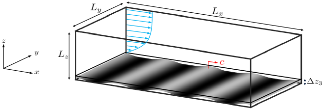
The computational domain is shown in Fig. 2. The prescribed wave motion shown is a monochromatic wave (later more general cases will be considered), with a wave amplitude , wavelength , and wave phase speed . Figure 2 also shows the wall model height, the height of the third vertical grid point , where the air velocity is taken for the equilibrium portion of the model. For applicability of the EQM, the wave cannot be higher than , therefore we enforce , where is the amplitude for a monochromatic wave. The vertical computational domain height is set equal to and all length-scales are normalized by such that . The streamwise and spanwise domain sizes are chosen such that at least a minimum of 4 waves exist in the domain and is not smaller that . Moreover, each wavelength is resolved in the horizontal direction by a minimum of 8 grid points.
For validation of the MOSD model in LES, we have selected seven previous studies; five are numerical and two are experimental. These particular validation cases were selected because they cover a meaningful range of wave parameters and contain sufficient information to perform comparisons with our LES. Data from computational studies by Wang et al. (2021), Zhang et al. (2019), Cao and Shen (2021) and Hao et al. (2021) are used. They perform WRLES of turbulent airflow over a smooth monochromatic wave at the bottom boundary using a time-dependent boundary fitted grid. We also compare with numerical data from Wu et al. (2022) who solve fully coupled wind forced water waves using DNS with a geometric volume of fluid method to reconstruct the interface. The experimental datasets used are from Buckley et al. (2020) and Yousefi et al. (2020). They performed high-resolution Particle Image Velocimetry (PIV) measurements of the turbulent airflow in close vicinity of the wavy interface.
| Reference | |||||
|---|---|---|---|---|---|
| 0.10 | 2.00 | 1133 | Wang et al. (2021) | ||
| 0.14 | 19.3 | 5000 | Hao et al. (2021) | ||
| 0.14 | 7.70 | 5000 | % | ||
| 0.10 | 7.25 | 1100 | Zhang et al. (2019) | ||
| 0.10 | 23.8 | 1110 | % | ||
| 0.06 | 6.57 | 1320 | Buckley et al. (2020) | ||
| 0.12 | 3.91 | 3025 | % | ||
| 0.17 | 2.62 | 5673 | % | ||
| 0.20 | 1.80 | 9598 | % | ||
| 0.26 | 1.53 | 10588 | Yousefi et al. (2020) | ||
| 0.20 | 8.00 | 720 | Wu et al. (2022) | ||
| 0.15 | 3.46 | 434 | Cao and Shen (2021) | ||
| 0.15 | 15.4 | 384 | % | ||
| 0.15 | 54.3 | 332 | % |
The data from Buckley et al. (2020) and Yousefi et al. (2020) were obtained at a large fetch such that the wavefield was sufficiently developed and reached fetch-limit equilibrium state. Furthermore, for all of their experimental cases, parasitic capillary waves are non-existing or their induced effect on the airflow is negligible. Therefore, for all validation cases, a smooth monochromatic wave is assumed (i.e. ). Table 1 summarizes the important wave parameters, as well as the domain size and numerical resolution used in our WMLES for each validation case.
4 Model Validation
In order to test the new wall model, LES of turbulent boundary layer flow over monochromatic waves are conducted and directly compared against numerical and experimental data shown in Table 1.
4.1 Turbulence Statistics: Mean Velocity and Reynolds Stress Profiles
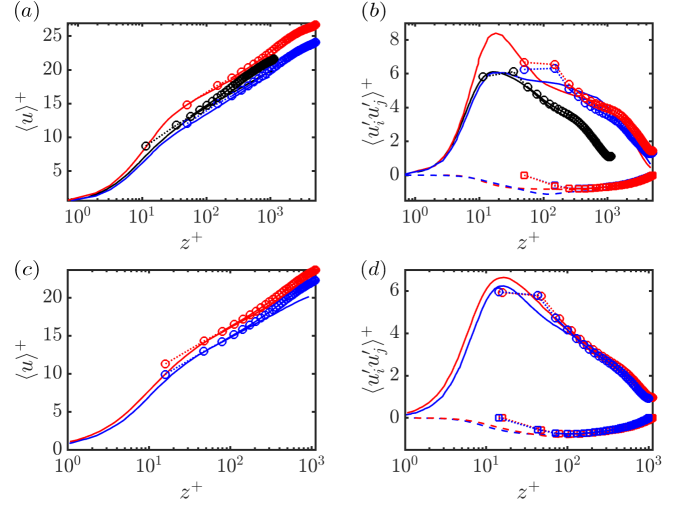
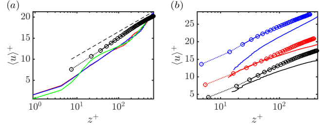
We compare first order and second order turbulence statistics of turbulent airflow above waves modeled using the MOSD approach in wall modeled LES. For some cases, due to data availability the second order statistics are not compared. First, in Fig. 3 we compare LES using the MOSD wall model with the WRLES data from Wang et al. (2021), Hao et al. (2021) and Zhang et al. (2019). In these LES monochromatic waves are represented by a moving boundary-fitted grid on the bottom of the numerical WRLES domain. For all of these cases, the mean streamwise velocity profiles from the wall modeled LES using the MOSD approach agree well with the WRLES datasets. The velocity profiles follow the law of the wall and compare well with the data in the logarithmic region, with a small overshoot in the wake region near the upper portion of the profile (where the effects of the wall model are negligible and instead results depend mostly on the subgrid scale model (Wang et al. 2020a), grid resolution and grid aspect ratio (Lozano-Durán and Bae 2019)). Several wave ages () are included in the comparisons of Fig. 3. A wave can be considered to be a high velocity wave (swell) if the wave age is larger than 25 (Smedman et al. 1994; Deskos et al. 2021). The case of Zhang et al. (2019) where and the Hao et al. (2021) case where can be considered moderate wave age cases. For moderate wave ages the wave velocity can become comparable to the wind velocity, thus, drag is greatly diminished leading to larger mean velocity when scaled with friction velocity. This trend is observed for the high case in the Hao et al. (2021) data in Fig. 3c. For faster wave age conditions, the wave velocity is usually higher than the airflow velocity (such a case will be examined later), thus, the wave can energize the flow instead of acting to deplete momentum in the air. In terms of second-order statistics (panels (b) and (d) in Fig.3), there is good agreement between the present results and the reference datasets except for the points nearest to the bottom surface, where some overestimation can be observed.
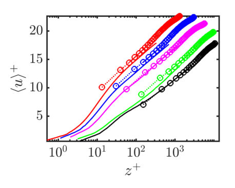
Figure 4 shows a comparison of mean velocity profiles from MOSD-based WMLES and the various experimental datasets from Buckley et al. (2020); Yousefi et al. (2020). The LES correctly reproduces the approximately logarithmic behavior and the amount of drag imparted to the wind (i.e., it provides good predictions of the velocity reduction below smooth surface behavior) for all conditions considered. A slight overprediction of the velocity profile (slight underprediction of the drag experienced due to the waves) is visible for two of the cases ( and ) but considering the range of conditions covered and the fact that no parameters are being adjusted from case to case, we consider the agreement quite good.
Next, we compare our MOSD-based wall modeled LES with the DNS data generated by Wu et al. (2022), where wind wave growth was investigated using a two-fluid method. In their work, the wave shape is initialized as a third-order Stokes wave whose parameters evolve as the wind and wave interact over time. We choose to validate against their and case over their specific non-dimensional time range (), where the wave parameters and form drag remain relatively constant. Figure 5a shows the comparison of the mean streamwise velocity profile from our LES with the Wu et al. (2022) DNS data. In this case the agreement is relatively poor, and it appears that the WMLES underpredicts the mean drag force acting on the wind. Considering that the study done by Wu et al. (2022) fully resolves all scales and coupling effects occurring at the air-water interface and that the their velocity profiles are not streamwise-averaged, one may expect some differences between the LES and the DNS data. Furthermore, we include a smooth profile (dashed line) to the Fig. 4b just as reference showing that the WMLES based on MOSD produces additional drag from the wave but insufficiently compared to this particular DNS.
In order to test the performance of the MOSD wall model for the case of fast moving waves that impart momentum to the wind above, we compare with data from Cao and Shen (2021). They use WRLES with a boundary fitted grid to solve for turbulent airflow over propagating waves with various phase speeds in a Couette flow setup. They include three cases of a slow, moderate and fast moving wave. The three cases have the same wave steepness to isolate the effects of the wave age. We simulate only the lower half of their domain (i.e. we consider to be the half-channel scale). Results are shown in Fig. 5b. For the intermediate case, the model correctly predicts the velocity profile in the inner part of the profile, i.e., a reduction in drag as the wave age approaches the moderate regime. Differences near the channel center are to be expected since we are not simulating Couette flow. Furthermore, for the fast moving wave () the MOSD-based WMLES predicts the addition of momentum to the wind. However, for this extreme condition the model overpredicts the momentum input from the wave to the wind thus overpredicting the velocity in the log-law region compared to the data. The slow wave age case also presents some differences between our WMLES and the comparison DNS data. It is worth noting that the data from Cao and Shen (2021) is at a moderate Reynolds number () for which additional effects may need to be considered. Still, one can argue that the MOSD model predicts the main qualitative trends quite successfully.
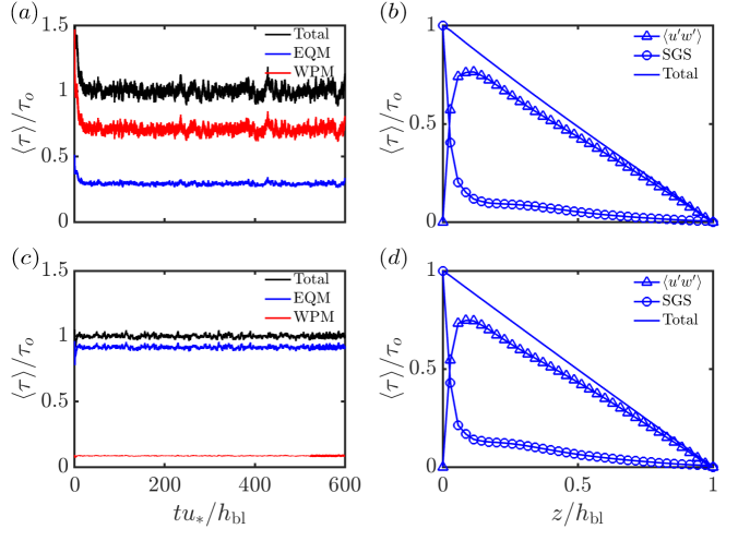
To illustrate the behavior of the MOSD model components for different wave parameters as well as their level of temporal fluctuations, Fig. 6 shows time signals of the total wall stress alongside the EQM and WPM components, normalized by the mean total wall stress (). Only two cases are shown, which represent widely different cases in terms of wave parameters (see Table 1). For both these cases the total wall stress fluctuates around its mean unit value, verifying that the balance between the wall stress and the nondimensional imposed pressure gradient. In Fig. 6a, the WPM dominates and represents approximately 60 of the total wall stress. This is expected because of the high wave steepness of this case (), corresponding to Yousefi et al. (2020). Conversely, for the Zhang et al. (2019) case (Fig. 6c) the contribution of the WPM component is approximately 1 of the total stress. In this case, although the wave velocity is higher compared to the case presented in Yousefi et al. (2020), for the specific Reynolds number of the airflow and with a wave steepness that is 2.6 times smaller, the contribution of the WPM would effectively be very small. The Reynolds and subgrid scale shear stress from MOSD-based WMLES for both reference cases are shown in Fig. 6b and Fig. 6d. For both, the dominant contribution is the resolved stress starting from 0 at wall and increasing linearly towards the half-channel height. The subfilter stress decreases from the wall towards the half-channel height, and starts becoming negligible in terms of the total stress around .
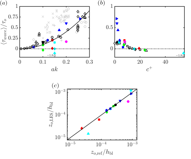
In order to place our WMLES results using MOSD in the context of results available in the literature, we show the stress fraction from the windward potential flow model normalized by the total wind stress plotted as function of wave steepness alongside data from a range of prior studies in Fig. 7a. The stress fraction has often been argued to scale as for small wave steepness and the proposed windward potential flow model follows this scaling since for monochromatic waves . However, the literature shows significant scatter since the stress fraction not only depends on wave steepness but also on wave age, Reynolds number and other effects. As is visible in Fig. 7a our MOSD-based wall modeled LES similarly displays significant scatter and does not fall on a single line. Figure 7b shows the normalized wave form drag as a function of the wave age also compared to cases in the literature. We observe how the wave drag fraction decreases as the wave age increases, for both the MOSD-based wall modeled LES as well as for the available literature data. Figure 7c shows a comparison of the surface roughness from the WMLES and the reference datasets. The solid line is where . The was obtained by fitting the data in the log-law region () using a least square method with prescribed slope ( and we use ) to determine the intercept. We observe a good agreement between the MOSD-based WMLES and the majority of the comparison data.
4.2 Phase-averaged and Wave-induced Motions
The prior validation analysis based on mean velocity and Reynolds stress profiles did not specifically highlight the phase-resolving features of the model. For that purpose, we next employ phase-averaging (Hussain and Reynolds 1970) to compare results from the the MOSD-based WMLES to data from prior phase resolving studies. Phase averaging allows us to isolate and analyze the specific motions and structures that are induced by the presence of surface waves. The triple decomposition of an arbitrary random signal (Hussain and Reynolds 1970) is given by:
| (22) |
where is the ensemble average component, denotes the wave-induced component that depends on phase , and is the uncorrelated (random) turbulent component. The average is obtained by averaging over all horizontal directions and time, i.e., over . The wave-induced component is given by , where is computed from:
| (23) |
where is the period of the wave, and the subscript denotes averaging over the spanwise direction.
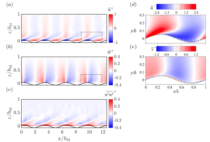
Contours of the normalized wave-induced horizontal and vertical velocities calculated by the MOSD-based WMLES for the Zhang et al. (2019) validation case are shown in Fig. 8a and Fig. 8b, respectively. Results are shown for the phase corresponding to the wave position shown in the figure. Here, the horizontal and vertical induced motions are positive on the windward side and negative on the leeward side of the wave. This behavior indicates that the airflow above accelerates as it passes over the windward face and later decelerates as it goes towards the leeward face, which is clearly consistent with the so-called “pumping”effect (Sullivan et al. 2008). The flow also accelerates directly above the crest (Buckley and Veron 2016).
These results indicate that the wave-induced structures of the horizontal and vertical velocities simulated in MOSD-based WMLES agree qualitatively with the results presented in Zhang et al. (2019). However, it can be seen that the WMLES predict an earlier onset of acceleration very near the surface in the troughs/valleys compared to the Zhang et al. (2019) WRLES comparison data, which instead show a negative streamwise wave-induced velocity near the wave. Also, we note that the amplitudes of the phase-averaged motions are underpredicted compared to the data by a factor of approximately 2-3. The MOSD model is built to be used specifically as a boundary condition for the horizontal velocity component, hence the vertical velocity is not directly affected by the boundary condition. The observed vertical motions in Fig.8b are a result of the divergence-free condition of the flow. When the airflow approaches the windward side of the wave, volume conservation dictates that the flow must move upwards. While this effect is not reproduced at a quantitative level, it is reproduced qualitatively and compared to the full velocity, the discrepancy is relatively small (on the order of only).
Finally, we examine the turbulent stress caused by the presence of the waves (wave-induced turbulent stress). The wave-induced turbulent stress is defined as:
| (24) |
where, is the phase-averaged component and is the horizontal and time average of the shear stress. The wave-induced Reynolds shear stress obtained from MOSD-based WMLES for the Zhang et al. (2019) case is shown in Fig. 8c. A positive stress appears very near the surface of the wave on the windward side, extending towards the crest. On the leeward side of the wave, negative shear stress is observed, creating a positive-negative pattern along the wave crests. The negative values are tilted and are found always downwind of the the wave, the positive values are also tilted and can extend towards the windward side of the next wave. This positive-negative pattern extends vertically until . The wave-induced turbulent shear stress behavior found using the MOSD-based WMLES shows good qualitative agreement with the trends obtained in the experiments by Yousefi et al. (2020).
The results shown illustrate the performance of the MOSD wall modeling approach in LES: it can represent phase-averaged overall drag effects reasonably accurately over a range of wave parameters, and captures qualitative features as function of wave phase. This performance is achieved at significant computational savings compared to phase and wall-resolved LES. For example, in the WRLES Zhang et al. (2019) case, the streamwise grid size remains uniformly resolved with a resolution of , while in the vertical direction, the grid size ranges from to . In comparison, LES with MOSD wall model for this case employs a grid size resolution of and . This difference in resolution requirements translates to a significant reduction in computational cost, a factor of between (obtained as , assuming a similar ratio in spanwise resolutions and also taking into account the reduced time-stepping requirements of WMLES).
5 Applicability Beyond Monochromatic Aligned Waves
In the previous section we have shown how the MOSD-wall model can capture mean and phase effects for simple waves (monochromatic, single phase velocity aligned with the mean wind direction). In reality, ocean waves are multiscale, i.e., a superposition of many waves with different wave lengths and phase velocities. To capture the impact of such multiscale waves on the ABL, the MOSD model relies on the local slope as determined from and based on (7) for evaluating the general velocity of the surface. It is therefore applicable in principle to any wave spectrum and wave phase velocity direction. To illustrate applicability of the MOSD model to waves beyond single wave-length, wind-aligned cases, we choose three cases. The first scenario corresponds to two distinct waves with different wave steepness moving in the same direction but at different phase velocities. The second scenario is of a single wave moving at an angle relative to the wind (oblique waves) at a fixed phase velocity. The third scenario represents two distinct waves, both moving at an angle with respect to the wind and at different phase velocities. Figure 9 illustrates the three different scenarios.
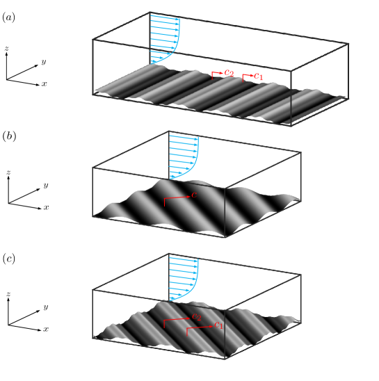
Table 2 summarizes the wave parameters, numerical domain and resolution for each of the cases considered. We choose to use the Zhang et al. (2019) case of and as a base case for comparison purposes. For these illustrative applications of the MOSD wall model, there are no literature data for us to compare with, so the simulation results are shown to demonstrate that the model can be applied to such cases and that it predicts trends that are as expected and physically meaningful.
For the first scenario of double aligned waves (DAW) we consider two cases. For the first case (DAW07), the second wave has a small steepness of . For the second case (DAW15), the second wave has a bigger steepness . For both cases, the phase velocity of the second wave is the same. For the second scenario we consider two cases of single misaligned waves (SMW). For the first case (SMW45) the wave moves at with respect to the mean wind direction. In the second case (SMW90), the wave moves at , i.e., completely perpendicular to the mean wind direction. For the third scenario, where we have double misaligned waves (DMW), only one case is simulated. In this case, the second wave has the same parameters as DAW15 and both waves are moving at angle with respect to the incoming wind. In all the cases shown in Table 2 have the same primary wave (wave 1) in terms of steepness and phase velocity (same as the Zhang et al. (2019) reference case).
| Case | |||||||
|---|---|---|---|---|---|---|---|
| DAW07 | 0.1 | 7.25 | 0.07 | 1 | |||
| DAW15 | 0.1 | 7.25 | 0.15 | 1 | |||
| SMW45 | 0.1 | 7.25 | 0 | 0 | |||
| SMW90 | 0.1 | 7.25 | 0 | 0 | |||
| DMW | 0.1 | 7.25 | 0.15 | 1 |
To first visualize the effects of different wave scenarios onto the turbulence near the surface, instantaneous contours of streamwise velocity component normalized by the friciton velocity at the wall model height (the third vertical grid point above the bottom surface) are shown in Fig. 10.
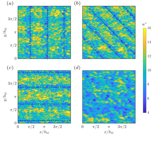
The presence of the waves is visible as a decrease in velocity in the form of bands, which in the near-surface region is correlated with the crests of the wave (as discussed in Sect. 4.2, the trend is reversed and the flow preferentially accelerates above the crest of the waves). For the DMW case, the presence of waves is difficult to observe because this case has two waves of distinct sizes, however, some remnant effects of the primary wave can be observed. These visualizations also further demonstrate the phase-dependent effects captured using the MOSD model.
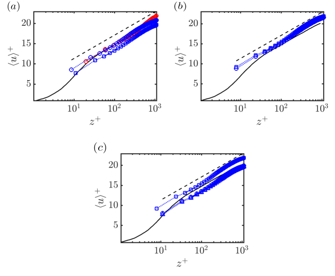
Figure 11a shows the mean streamwise velocity profile for the first scenario consisting of two aligned waves (DAW07 and DAW15 cases). We expect that two waves would increase the amount of drag being imparted onto the airflow above. However, only the DAW15 case shows a clear offset of the velocity profile characteristic of an increase in drag. For the DAW07 case, the drag imparted is virtually the same as the drag created from only one wave. This can be explained by noting that it’s steepness is less than the primary wave, and since the drag scales by , the second wave becomes negligible in terms of drag.
Figure 11b shows the mean streamwise velocity profile comparison for cases SMW45 and SMW90. Here, we observe that there is less drag being imparted onto the airflow versus the wind and wave aligned case Zhang et al. (2019), therefore a positive offset in the log-layer region is observed. This decrease in drag is clearly due to the angle between wind and wave since both cases have the same wave parameters as the Zhang et al. (2019) case. This behavior is consistent with studies by Karniadakis and Choi (2003); Tomiyama and Fukagata (2013); Ghebali et al. (2017), where transverse motions created by passive means like wall oscillation and transverse traveling walls have been found to create some drag reduction of turbulent boundary layer flows.
The mean streamwise velocity for the DMW case is shown in Fig. 11c. The drag generated differs slightly from that in the DAW15 case. Considering the results obtained in Fig. 11b, it seems logical to infer that although the present case and DAW15 case have the same wave parameters, the slight difference in velocity profile offset is due entirely to the wave direction with respect to the wind.
6 Comparison with Wind Tunnel Data for Offshore Wind Turbine
In the previous sections, we have tested the accuracy and general applicability of the MOSD wall model in LES to predict air flow over moving waves of various types. This wall-modeling approach offers a cost-effective method for capturing the influence of waves on the ABL including phase-dependent information. In this section, we explore the applicability of the MOSD wall model to LES of offshore wind turbine wake flow. Specifically, a comparison with data from a recent laboratory experiments for the case of a fixed bottom offshore wind turbine is presented.
6.1 Experimental Setup
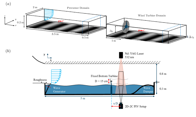
The experiments for a scaled fixed bottom wind turbine (Ferčák et al. 2022) were performed in the closed loop wind and water tunnel at Portland State University (PSU). The wind tunnel test section had a height of 0.8 m, width of 1.2 m and test-length of 5 m. The wind tunnel speed (free-stream velocity) was fixed at 6 m/s. The tunnel ceiling was configured to produce a nominally zero-pressure gradient boundary layer. The water tank covered the full wind tunnel floor and provided a water depth of 0.3 m. A wave paddle was positioned at the entrance of the test-section and was controlled by a stepper motor to produce scaled deepwater waves. Since the focus is solely on the effect of waves on wake development, an idealized setup using unidirectional waves was used to focus the study on the flow interactions between turbulence and a single wavelength wave. Based on the wind tunnel size, a diameter of 0.15 m was selected for the scaled wind turbine, resulting in a geometric scaling ratio of 1:600 in comparison to a full scale turbine with (e.g.) a diameter of 90 m. The size of the turbine model and resulting Reynolds number is sufficiently high to show realistic wake dynamics (Chamorro et al. 2012). The water tank depth of 0.3 m corresponds to 180 m in full-scale. It is noted that a 180 m water depth is in a range relevant to floating wind turbines since it is well beyond the approximately 50 m limit for current fixed bottom turbines. A schematic representation of the experimental set up is included in Fig. 12.
The model turbine thrust coefficient was measured using a uni-axial load cell on the turbine rotor at the tip speed ratio () used in the experiment. The wave paddle was set to a frequency resulting in a wave with a measured period of () s. The measured wave speed () generated by the paddle was () m/s, and the measured wavelengths () was () m. The water surface elevation (the interface between wind and wave) was measured with Light-Induced Fluorescence (LIF). Particle Image Velocimetry (PIV) was used to measure 2D velocity fields in streamwise aligned () planes. The friction velocity fitted from the mean velocity profile and using a von Karman constant of was found to be m/s. The boundary layer height in the region of the turbine was approximately m. More detailed information regarding the experimental set up can be found in Ferčák et al. (2022).
6.2 MOSD-based WMLES Simulation Setup
We simulate wind-wave-wake dynamics numerically using the same procedure described in 3.2 for wind-wave interaction with a wind turbine introduced into the numerical domain. Figure 12a shows the computational domain used.The effect of the wind turbine rotor on the wind is modeled using the actuator-disk model (ADM), which is commonly applied to the study of land-based wind farms (Calaf et al. 2010; Shapiro et al. 2019) and offshore wind farms (Yang et al. 2014c, b). We use a local thrust coefficient (allowing us to use the disc-averaged air velocity instead of a far upstream reference velocity (Meyers and Meneveau 2010)) of , which is computed from , where is used to represent the turbine rotor induction (Calaf et al. 2010). We also include a model for the drag caused by the model turbine nacelle at the grid points near the turbine center using a drag coefficient of (this value was selected aiming to create a velocity deficit near the turbine similar to that of the experiment). The simulation of wind-wave-turbine is performed using two computational domains, a precursor and a wind turbine domain (Stevens et al. 2014). The turbine is placed in the wind turbine domain while the turbulent inflow conditions are generated in the precursor domain. The domain height (half-channel scale in the idealized version of the experiment) is set to equal the boundary layer height, i.e. m. The usual air viscosity m2/s is used and the Reynolds number of the wind tunnel experiments is matched by selecting the forcing pressure gradient to correspond to the measured friction velocity m/s.
The MOSD wall model is applied to both the precursor and wind turbine domains. A shifted periodic boundary condition (Munters et al. 2016) is used in the streamwise direction of the precursor domain to prevent artificially long flow structures from developing. In the concurrent-precursor method (Stevens et al. 2014) the turbulence and velocity developed in the precursor is then used as an inflow condition to the wind turbine domain. At at each time step, a part of flow from the precursor domain is copied to the outflow region of the wind turbine domain. A fringe region is then defined to smoothly transition between the wind turbine flow and the region of flow copied from the precursor domain and the prescribed “outflow” in the wind turbine domain is then equal to the inflow to this domain owing to the periodic boundary conditions used in the pseudo-spectral method in the horizontal directions.
| (m) | |||||
|---|---|---|---|---|---|
| 0.08 | 4.44 | 0.2 |
Table 3 summarizes the wave parameters from the experiment and the numerical resolution used for the wall-modeled LES. The experiments exhibited small wind driven waves (ripples) on top of the primary wave which was generated by the paddle. These small scale waves could not be horizontally resolved with the current LES grid, therefore, they are modeled as a surface roughness using Eq.15. By means of light-induced fluorescence (LIF), the r.m.s size of the ripples was measured to be m , which represents roughly 6% of the amplitude of the wave-maker generated wave. Since we want to include these unresolved ripples as a surface roughness in addition to including viscous effects on the surface, we use Eq. 11 with determined using Eqs. 12 and 13.
6.3 Results
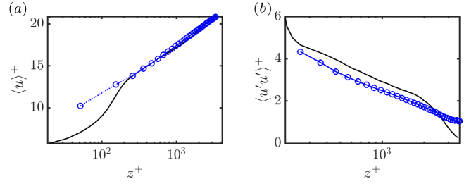
First, a LES of only wind over waves using the MOSD wall model was undertaken to verify that the turbulent inflow conditions from LES match those of the experiments. Figure 13 shows a comparison of measured mean velocity and streamwise velocity variance from experiments and the LES. Similarly to the validation cases shown in previous sections, the MOSD-based WMLES results show good agreement with the turbulent statistics of the airflow in the presence of the waves, especially in the logarithmic region of the mean velocity profile.
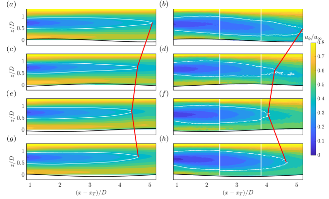
To isolate the turbine wake motions specifically induced by the presence of surface waves, phase averaged streamwise velocity contours of the downstream velocity in the near and intermediate wake region are compared from the MOSD-based WMLES and the experiments. The phase averaging is performed at four distinct phases ). For reference, is the phase in which the crest of the wave is located immediately under the turbine rotor location (). Results comparing LES and experiments in the near wake region starting one diameter downstream of the turbine up to about five diameters downstream are shown in Fig. 14. The wake in the LES is slightly weaker and thinner than in the experiments and appears more horizontal than the experimental wake, which has a slight downward tilt. Differences due to the LES representation of the nacelle (which is significant in the wind tunnel setup) and in outer flow conditions (boundary layer in the experiments versus half-channel in LES) are expected and likely to contribute to observed differences in wake properties. However, in terms of trends with respect to the wave passage, there is good agreement. At each phase, we observe that in the some concavity in the lower regions of the wake exactly where the crest of the wave is located, this behavior is best observed for . Elevated velocity regions near the wave at the bottom part of the turbine are also observed, these high velocity regions are elongated and follow the wave crest extending towards the trough of the wave. Interestingly, both the experimental and LES results indicate that as the wave passes underneath the wake downstream, the wake compresses and shortens in the streamwise direction. The wake is longest at phase , e.g., consider the contour at a velocity of of the free-stream velocity highlighted with the white line. There the wave crest is near the turbine at . However, the wake then becomes shorter as the wave crest advances to and beyond. The red line shown in Fig. 14 for the WMLES marks the wake length at different phases for a fixed velocity threshold of . The compression and elongation of the length of the wake is primarily due to the pumping effect of the waves. As the wave moves, a horizontal velocity is induced onto the airflow above, increasing momentum and thus having an effect similar to wake recovery, or wake shortening at least for some of the time interval. This streching/compressing behavior of the wake can also be observed in the experimental data of Ferčák et al. (2022) shown in the panels to the right in Fig. 14.
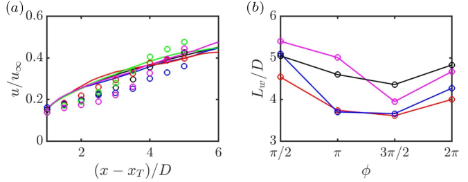
For further comparison between the numerical and experimental results, the wake velocity along the wake center as function of downstream distance from the turbine is calculated and shown in Fig. 15a. The wave steepness and velocity for this case can be considered “small” and “slow”, respectively, thus the vertical induced motions due to the wave movement are small but not negligible. Finally, the wake length at each phase is shown in Fig.15b. The experimental wake length was computed assuming three different threshold values of , and . For the numerical results only the wake length at a threshold of is shown, which is consistent with the behavior of the red line shown in Fig. 14. The maximum wave length is obtained at , while the minimum is at , for both the MOSD-based WMLES and the experimental data sets. After the wave crest advances from , the pumping effect is diminished and the wake size increases. This trend is consistent with the observations discussed before in Sect.4.2. Although there is good qualitative agreement, the observed remaining discrepancies between the WMLES phase-average results and the experiments are likely due to the model’s underestimation of the magnitude of vertical motions, as discussed in Sect.4.2.
7 Summary and Conclusions
Understanding and modeling the physical processes and mechanisms within the marine atmospheric boundary layer hinges on the accurate quantification of momentum transfer at the air-sea interface. Presently, numerical methodologies employed to study fundamental aspects of wind-wave interactions typically entail computationally intensive techniques such as DNS or WRLES coupled with terrain-following grids or high-order spectral methods (“wave-phase-resolved” approach) for resolving the wave. These approaches often incur prohibitively high computational costs and are difficult to implement in codes as simple boundary conditions, limiting their widespread applicability. Alternatively, effective roughness length scale-based methods (“wave-phase-averaged” approach) can be imposed to characterize the wind-wave interactions in LES. However, this methodology relies mostly on empirical parameters and does not enable the reproduction of any phase-dependent processes.
In this study, a moving surface drag (MOSD) model for LES is introduced that effectively captures phase-dependent effects of waves, while maintaining computational efficiency. The proposed model focuses on accurately resolving the net pressure force resulting from the interaction between moving surface waves and turbulent wind. This model builds upon the surface-gradient based wall model introduced by (Anderson and Meneveau 2010) that has also been extended to moving surfaces by Aiyer et al. (2023). The latter two approaches focus on the momentum flux of the air flow and assume that the entirety (or some modeled fraction) of the momentum is imparted onto the surface. In the present model, we extend the Anderson and Meneveau (2010) model along a different direction, namely by evaluating the potential flow pressure distribution on the windward facing side of the waves. Its integration yields the form drag (pressure force), which can be cast as a wall stress boundary condition. Since the MOSD wall model is based on mechanistic principles, it does not in principle require further calibration or adjustments of empirical prefactors or adjustable parameters.
The model was validated against several experimental and numerical benchmark cases of turbulent boundary layer air flow over monochromatic moving waves. The MOSD model successfully captured the impact of waves on the mean velocity profile of the airflow across the majority of the test cases. However, while wave-induced structures show qualitative agreement with the comparison data, the strength of vertical motions is underpredicted by the model and future efforts should be focused on developing modifications to fully capture the induced vertical motions. To illustrate the applicability of the model to cases more complex than single wavelength and wind aligned waves, several such scenarios were simulated, demonstrating that the model effectively captures expected trends in such cases. We leave consideration of fully broadband wave fields for future work.
Finally, a fixed-bottom offshore turbine was simulated in LES using the MOSD model to represent the waves and results were compared to wind tunnel experimental data. Results confirm that features from copupled wind-wave-wake dynamics can be captured, specifically the stretching/compressing of the wake as the wave passes through.
It is useful to underline the strong modeling assumptions that have been made in deriving the MOSD wall model. The modeling of unresolved roughness or the smooth wall viscous layer using the equilibrium model can be justified reasonably well. While its underlying assumptions can be questioned (see e.g. the literature review and arguments presented in Fowler et al. (2022)), it is a well-established methodology with many successful applications in geophysical and engineering flows. Conversely, the windward potential flow model is based on the pressure distribution of a potential ramp flow over a moving surface represents a strong idealization of the real flow conditions that can be expected near a moving wave. One important approximation is the use of potential flow. The real flow is turbulent and thus differences can be expected. However, possibly the strongest assumption is that in each LES cell that contains portions of the wave surface there exists an idealized ramp flow. In particular, we assume that the flow impinges horizontally upon the surface, separately and independently in each cell. Referring back to Fig. 1(b), to the left of the cell shown there is in reality another cell where the flow could be deflected and arrive in a direction different than horizontal. To capture more realistically the near-surface flow even assuming potential flow would require taking into account non-local information, e.g., using a partial differential equation approach. For simplicity we purposefully limit the model to be entirely local and based only on quantities that are known at the cell where the wall model has to be evaluated. Under these constraints, the proposed model appears to be as accurate as can be expected. Its merits can be judged from the level of accuracy of the results presented. While the initial application of MOSD wall model in LES show encouraging results, subsequent tests should be focused on the applying the MOSD approach in LES of large offshore wind farms also including realistic ocean spectrum waves.
Acknowledgements.
The support of the Percy Pierre Graduate Fellowship from Johns Hopkins University, and National Science Foundation grants # CMMI-2034111, CMMI-2034160, CBET-2227263, and CBET-2037582 are gratefully acknowledged.References
- Aiyer et al. (2023) Aiyer AK, Deike L, Mueller ME (2023) A sea surface–based drag model for large-eddy simulation of wind–wave interaction. Journal of the Atmospheric Sciences 80(1):49 – 62
- Åkervik and Vartdal (2019) Åkervik E, Vartdal M (2019) The role of wave kinematics in turbulent flow over waves. Journal of Fluid Mechanics 880:890–915
- Al-Zanaidi and Hui (1984) Al-Zanaidi MA, Hui WH (1984) Turbulent airflow over water waves-a numerical study. Journal of Fluid Mechanics 148:225–246, DOI 10.1017/S0022112084002329
- Albertson and Parlange (1999) Albertson J, Parlange M (1999) Surface length scales and shear stress: Implications for land-atmosphere interaction over complex terrain. Water Resources Research 35(7):2121–2132, DOI https://doi.org/10.1029/1999WR900094
- Anderson and Meneveau (2010) Anderson W, Meneveau C (2010) A large-eddy simulation model for boundary-layer flow over surfaces with horizontally resolved but vertically unresolved roughness elements. Boundary-Layer Meteorology 137(3):397–415, DOI 10.1007/s10546-010-9537-5
- Banner (1990) Banner ML (1990) The influence of wave breaking on the surface pressure distribution in wind—wave interactions. Journal of Fluid Mechanics 211:463–495, DOI 10.1017/S0022112090001653
- Banner and Peirson (1998) Banner ML, Peirson WL (1998) Tangential stress beneath wind-driven air–water interfaces. Journal of Fluid Mechanics 364:115–145, DOI 10.1017/S0022112098001128
- Bou-Zeid et al. (2005) Bou-Zeid E, Meneveau C, Parlange M (2005) A scale-dependent lagrangian dynamic model for large eddy simulation of complex turbulent flows. Physics of Fluids 17(2):025,105, DOI 10.1063/1.1839152
- Buckley and Veron (2016) Buckley MP, Veron F (2016) Structure of the airflow above surface waves. Journal of Physical Oceanography 46(5):1377 – 1397
- Buckley et al. (2020) Buckley MP, Veron F, Yousefi K (2020) Surface viscous stress over wind-driven waves with intermittent airflow separation. Journal of Fluid Mechanics 905:A31, DOI 10.1017/jfm.2020.760
- Calaf et al. (2010) Calaf M, Meneveau C, Meyers J (2010) Large eddy simulation study of fully developed wind-turbine array boundary layers. Physics of fluids 22(1):015,110
- Cao and Shen (2021) Cao T, Shen L (2021) A numerical and theoretical study of wind over fast-propagating water waves. Journal of Fluid Mechanics 919:A38, DOI 10.1017/jfm.2021.416
- Chamorro et al. (2012) Chamorro L, Arndt R, Sotiropoulos F (2012) Reynolds number dependence of turbulence statistics in the wake of wind turbines. Wind Energy 15(5):733–742, DOI https://doi.org/10.1002/we.501
- Charnock (1955) Charnock H (1955) Wind stress on a water surface. Quarterly Journal of the Royal Meteorological Society 81(350):639–640, DOI https://doi.org/10.1002/qj.49708135027
- Deskos et al. (2021) Deskos G, Lee J, Draxl C, Sprague M (2021) Review of wind–wave coupling models for large-eddy simulation of the marine atmospheric boundary layer. Journal of the Atmospheric Sciences 78(10):3025 – 3045, DOI 10.1175/JAS-D-21-0003.1
- Deskos et al. (2022) Deskos G, Ananthan S, Sprague MA (2022) Direct numerical simulations of turbulent flow over misaligned traveling waves. International Journal of Heat and Fluid Flow 97:109,029
- Donelan et al. (2006) Donelan MA, Babanin AV, Young IR, Banner ML (2006) Wave-follower field measurements of the wind-input spectral function. part ii: Parameterization of the wind input. Journal of Physical Oceanography 36(8):1672 – 1689
- Edson et al. (2007) Edson J, Crawford T, Crescenti J, Farrar T, Frew N, Gerbi G, Helmis C, Hristov T, Khelif D, Jessup A, Jonsson H, Li M, Mahrt L, McGillis W, Plueddemann A, Shen L, Skyllingstad E, Stanton T, Sullivan P, Sun J, Trowbridge J, Vickers D, Wang S, Wang Q, Weller R, Wilkin J, Williams AJ, Yue DKP, Zappa C (2007) The coupled boundary layers and air–sea transfer experiment in low winds. Bulletin of the American Meteorological Society 88(3):341 – 356
- Ferčák et al. (2022) Ferčák O, Bossuyt J, Ali N, Cal RB (2022) Decoupling wind–wave–wake interactions in a fixed-bottom offshore wind turbine. Applied Energy 309:118,358, DOI https://doi.org/10.1016/j.apenergy.2021.118358
- Fowler et al. (2022) Fowler M, Zaki TA, Meneveau C (2022) A lagrangian relaxation towards equilibrium wall model for large eddy simulation. Journal of Fluid Mechanics 934:A44
- Funke et al. (2021) Funke CS, Buckley MP, Schultze LKP, Veron F, Timmermans MLE, Carpenter JR (2021) Pressure fields in the airflow over wind-generated surface waves. Journal of Physical Oceanography 51(11):3449 – 3460, DOI https://doi.org/10.1175/JPO-D-20-0311.1
- Gent and Taylor (1976) Gent PR, Taylor PA (1976) A numerical model of the air flow above water waves. Journal of Fluid Mechanics 77(1):105–128, DOI 10.1017/S0022112076001158
- Geva and Shemer (2022) Geva M, Shemer L (2022) Wall similarity in turbulent boundary layers over wind waves. Journal of Fluid Mechanics 935:A42, DOI 10.1017/jfm.2022.54
- Ghebali et al. (2017) Ghebali S, Chernyshenko SI, Leschziner MA (2017) Can large-scale oblique undulations on a solid wall reduce the turbulent drag? Physics of Fluids 29(10), DOI 10.1063/1.5003617
- Grachev and Fairall (2001) Grachev A, Fairall C (2001) Upward momentum transfer in the marine boundary layer. Journal of physical oceanography 31(7):1698–1711
- Grare et al. (2013) Grare L, Peirson WL, Branger H, Walker JW, Giovanangeli JP, Makin V (2013) Growth and dissipation of wind-forced, deep-water waves. Journal of Fluid Mechanics 722:5–50, DOI 10.1017/jfm.2013.88
- Grare et al. (2018) Grare L, Lenain L, Melville WK (2018) Vertical profiles of the wave-induced airflow above ocean surface waves. Journal of Physical Oceanography 48(12):2901 – 2922
- Hao and Shen (2019) Hao X, Shen L (2019) Wind–wave coupling study using les of wind and phase-resolved simulation of nonlinear waves. Journal of Fluid Mechanics 874:391–425
- Hao et al. (2021) Hao X, Cao T, Shen L (2021) Mechanistic study of shoaling effect on momentum transfer between turbulent flow and traveling wave using large-eddy simulation. Phys Rev Fluids 6:054,608, DOI 10.1103/PhysRevFluids.6.054608
- Hussain and Reynolds (1970) Hussain AKMF, Reynolds WC (1970) The mechanics of an organized wave in turbulent shear flow. Journal of Fluid Mechanics 41(2):241–258, DOI 10.1017/S0022112070000605
- Jeffreys (1925) Jeffreys H (1925) On the formation of water waves by wind. Proceedings of the Royal Society of London Series A, Containing Papers of a Mathematical and Physical Character 107(742):189–206
- Karniadakis and Choi (2003) Karniadakis GE, Choi KS (2003) Mechanisms on transverse motions in turbulent wall flows. Annual Review of Fluid Mechanics 35(1):45–62, DOI 10.1146/annurev.fluid.35.101101.161213
- Kawai and Larsson (2012) Kawai S, Larsson J (2012) Wall-modeling in large eddy simulation: Length scales, grid resolution, and accuracy. Physics of Fluids 24(1):015,105, DOI 10.1063/1.3678331
- Kihara et al. (2007) Kihara N, Hanazaki H, Mizuya T, Ueda H (2007) Relationship between airflow at the critical height and momentum transfer to the traveling waves. Physics of Fluids 19(1):015,102, DOI 10.1063/1.2409736
- Kundu et al. (2015) Kundu P, Cohen I, Dowling D (2015) Fluid Mechanics, 6th edn, Elsevier
- Lamb (1945) Lamb H (1945) Hydrodynamics, 6th edn, Dover Publications
- LESGO (2022) LESGO (2022) Github webpage. http://e https://lesgo.me.jhu.edu.
- Li et al. (2000) Li P, Xu D, Taylor P (2000) Numerical modelling of turbulent airflow over water waves. Boundary-layer meteorology 95:397–425
- Lin et al. (2008) Lin MY, Moeng CH, Tsai WT, Sullivan PP, Belcher SE (2008) Direct numerical simulation of wind-wave generation processes. Journal of Fluid Mechanics 616:1–30, DOI 10.1017/S0022112008004060
- Longuet-Higgins (1963) Longuet-Higgins MS (1963) The generation of capillary waves by steep gravity waves. Journal of Fluid Mechanics 16(1):138–159, DOI 10.1017/S0022112063000641
- Lozano-Durán and Bae (2019) Lozano-Durán A, Bae HJ (2019) Error scaling of large-eddy simulation in the outer region of wall-bounded turbulence. Journal of computational physics 392:532–555
- Mastenbroek et al. (1996) Mastenbroek C, Makin VK, Garat MH, Giovanangeli JP (1996) Experimental evidence of the rapid distortion of turbulence in the air flow over water waves. Journal of Fluid Mechanics 318:273–302, DOI 10.1017/S0022112096007124
- Masuda and Kusaba (1987) Masuda A, Kusaba T (1987) On the local equilibrium of winds and wind-waves in relation to surface drag. Journal of the Oceanographical Society of Japan 43(1):28–36, DOI 10.1007/BF02110631
- Meneveau (2020) Meneveau C (2020) A note on fitting a generalised moody diagram for wall modelled large-eddy simulations. Journal of Turbulence 21(11):650–673
- Meyers and Meneveau (2010) Meyers J, Meneveau C (2010) Large Eddy Simulations of Large Wind-Turbine Arrays in the Atmospheric Boundary Layer. DOI 10.2514/6.2010-827, https://arc.aiaa.org/doi/pdf/10.2514/6.2010-827
- Moeng (1984) Moeng CH (1984) A large-eddy-simulation model for the study of planetary boundary-layer turbulence. Journal of Atmospheric Sciences 41(13):2052 – 2062
- Munters et al. (2016) Munters W, Meneveau C, Meyers J (2016) Shifted periodic boundary conditions for simulations of wall-bounded turbulent flows. Physics of Fluids 28(2):025,112, DOI 10.1063/1.4941912
- Narasimhan et al. (2022) Narasimhan G, Gayme DF, Meneveau C (2022) Effects of wind veer on a yawed wind turbine wake in atmospheric boundary layer flow. Phys Rev Fluids 7:114,609, DOI 10.1103/PhysRevFluids.7.114609
- Peirson and Garcia (2008) Peirson W, Garcia A (2008) On the wind-induced growth of slow water waves of finite steepness. Journal of Fluid Mechanics 608:243–274, DOI 10.1017/S002211200800205X
- Perlin et al. (1993) Perlin M, Lin H, Ting CL (1993) On parasitic capillary waves generated by steep gravity waves: an experimental investigation with spatial and temporal measurements. Journal of Fluid Mechanics 255:597–620, DOI 10.1017/S0022112093002605
- Piomelli and Balaras (2002) Piomelli U, Balaras E (2002) Wall-layer models for large-eddy simulations. Annual Review of Fluid Mechanics 34(1):349–374, DOI 10.1146/annurev.fluid.34.082901.144919
- Shapiro et al. (2019) Shapiro CR, Gayme DF, Meneveau C (2019) Filtered actuator disks: Theory and application to wind turbine models in large eddy simulation. Wind Energy 22(10):1414–1420, DOI https://doi.org/10.1002/we.2376
- Smedman et al. (1994) Smedman AS, Tjernström M, Högström U (1994) The near-neutral marine atmospheric boundary layer with no surface shearing stress: A case study. Journal of Atmospheric Sciences 51(23):3399 – 3411
- Smith et al. (1992) Smith SD, Anderson RJ, Oost WA, Kraan C, Maat N, De Cosmo J, Katsaros KB, Davidson KL, Bumke K, Hasse L, Chadwick HM (1992) Sea surface wind stress and drag coefficients: The hexos results. Boundary-Layer Meteorology 60(1):109–142, DOI 10.1007/BF00122064
- Snyder et al. (1981) Snyder RL, Dobson FW, Elliott JA, Long RB (1981) Array measurements of atmospheric pressure fluctuations above surface gravity waves. Journal of Fluid Mechanics 102:1–59, DOI 10.1017/S0022112081002528
- Stevens et al. (2014) Stevens RJ, Graham J, Meneveau C (2014) A concurrent precursor inflow method for large eddy simulations and applications to finite length wind farms. Renewable Energy 68:46–50, DOI https://doi.org/10.1016/j.renene.2014.01.024
- Stoll et al. (2020) Stoll R, Gibbs JA, Salesky ST, Anderson W, Calaf M (2020) Large-eddy simulation of the atmospheric boundary layer. Boundary-Layer Meteorology 177:541–581
- Sullivan et al. (2000) Sullivan PP, McWilliams JC, Moeng CH (2000) Simulation of turbulent flow over idealized water waves. Journal of Fluid Mechanics 404:47–85, DOI 10.1017/S0022112099006965
- Sullivan et al. (2008) Sullivan PP, Edson JB, Hristov T, McWilliams JC (2008) Large-eddy simulations and observations of atmospheric marine boundary layers above nonequilibrium surface waves. Journal of the Atmospheric Sciences 65(4):1225–1245
- Sullivan et al. (2018) Sullivan PP, Banner ML, Morison RP, Peirson WL (2018) Turbulent flow over steep steady and unsteady waves under strong wind forcing. Journal of Physical Oceanography 48(1):3 – 27, DOI https://doi.org/10.1175/JPO-D-17-0118.1
- Toba et al. (1990) Toba Y, Iida N, Kawamura H, Ebuchi N, Jones ISF (1990) Wave dependence of sea-surface wind stress. Journal of Physical Oceanography 20(5):705 – 721, DOI https://doi.org/10.1175/1520-0485(1990)020¡0705:WDOSSW¿2.0.CO;2
- Tomiyama and Fukagata (2013) Tomiyama N, Fukagata K (2013) Direct numerical simulation of drag reduction in a turbulent channel flow using spanwise traveling wave-like wall deformation. Physics of Fluids 25(10), DOI 10.1063/1.4826887
- Wang et al. (2020a) Wang L, Hu R, Zheng X (2020a) A comparative study on the large-scale-resolving capability of wall-modeled large-eddy simulation. Physics of Fluids 32(3):035,102
- Wang et al. (2020b) Wang LH, Zhang WY, Hao X, Huang WX, Shen L, Xu CX, Zhang Z (2020b) Surface wave effects on energy transfer in overlying turbulent flow. Journal of Fluid Mechanics 893:A21, DOI 10.1017/jfm.2020.246
- Wang et al. (2021) Wang LH, Xu CX, Sung HJ, Huang WX (2021) Wall-attached structures over a traveling wavy boundary: Turbulent velocity fluctuations. Phys Rev Fluids 6:034,611, DOI 10.1103/PhysRevFluids.6.034611
- Wu et al. (2022) Wu J, Popinet S, Deike L (2022) Revisiting wind wave growth with fully coupled direct numerical simulations. Journal of Fluid Mechanics 951:A18, DOI 10.1017/jfm.2022.822
- Yang and Shen (2010) Yang D, Shen L (2010) Direct-simulation-based study of turbulent flow over various waving boundaries. Journal of Fluid Mechanics 650:131–180, DOI 10.1017/S0022112009993557
- Yang et al. (2014a) Yang D, Meneveau C, Shen L (2014a) Effect of downwind swells on offshore wind energy harvesting – a large-eddy simulation study. Renewable Energy 70:11–23, DOI https://doi.org/10.1016/j.renene.2014.03.069
- Yang et al. (2014b) Yang D, Meneveau C, Shen L (2014b) Effect of downwind swells on offshore wind energy harvesting – a large-eddy simulation study. Renewable Energy 70:11–23
- Yang et al. (2014c) Yang D, Meneveau C, Shen L (2014c) Large-eddy simulation of offshore wind farm. Physics of Fluids 26(2):025,101
- Yang and Griffin (2021) Yang XIA, Griffin KP (2021) Grid-point and time-step requirements for direct numerical simulation and large-eddy simulation. Physics of Fluids 33(1), DOI 10.1063/5.0036515
- Yousefi et al. (2020) Yousefi K, Veron F, Buckley MP (2020) Momentum flux measurements in the airflow over wind-generated surface waves. Journal of Fluid Mechanics 895:A15, DOI 10.1017/jfm.2020.276
- Zhang et al. (2019) Zhang WY, Huang WX, Xu CX (2019) Very large-scale motions in turbulent flows over streamwise traveling wavy boundaries. Phys Rev Fluids 4:054,601, DOI 10.1103/PhysRevFluids.4.054601