Machine-learning structural reconstructions for accelerated point defect calculations

Abstract

Defects dictate the properties of many functional materials. To understand the behaviour of defects and their impact on physical properties, it is necessary to identify the most stable defect geometries. However, global structure searching is computationally challenging for high-throughput defect studies or materials with complex defect landscapes, like alloys or disordered solids. Here, we tackle this limitation by harnessing a machine-learning surrogate model to qualitatively explore the defect structural landscape. By learning defect motifs in a family of related metal chalcogenide and mixed anion crystals, the model successfully predicts favourable reconstructions for unseen defects in unseen compositions for 90% of cases, thereby reducing the number of first-principles calculations by 73%. Using CdSe_xTe_1-x alloys as an exemplar, we train a model on the end member compositions and apply it to find the stable geometries of all inequivalent vacancies for a range of mixing concentrations, thus enabling more accurate and faster defect studies for configurationally complex systems.

I Introduction

Defects control the properties of many functional materials and devices[1], like solar cells[2, 3], batteries[4, 5], catalysts[6, 7, 8], and quantum computers[9, 10, 11, 12]. To discover better materials for these applications it is thus necessary to predict how their defects behave. However, defect calculations are computationally demanding. The large supercells and high level of theory required to obtain robust predictions typically limit point defect analysis to in-depth studies of specific materials. In a move towards data-driven defect workflows[13], defect databases[14, 15, 16, 17, 18, 19, 20] and surrogate models have been developed to predict defect properties, like the dominant defect type[18], formation[21, 22, 23, 24, 25, 26, 27, 28, 29, 30, 31, 32, 33, 34, 35, 19] and migration[35] energies, and charge transition levels[36, 25, 19]. By learning the relationship between defect structure and properties, these models enable high-throughput studies that quickly evaluate and screen a group of materials based on their defect behaviour. [37, 27, 28, 30]

Despite progress in accelerating defect predictions, most high-throughput studies are limited in scope. Typically, their training datasets are generated assuming the ideal defect structure inherited from the crystal host, which often lies within a local minimum, thereby trapping a gradient-based optimisation algorithm in a metastable arrangement[38, 39, 40, 41]. By yielding incorrect geometries, the predicted defect properties, such as equilibrium concentrations[41, 42, 39], charge transition levels[41, 42, 39] and recombination rates[39], are rendered inaccurate.[43, 44, 45, 8, 46]. However, defect structure searching is often too expensive for high-throughput studies that target thousands of defects[30] or materials with complex (defect) energy landscapes, like alloys, disordered solids, and low-symmetry crystals.

In this study, we aim to reduce the computational burden of defect structure searching by introducing a machine-learning surrogate model. We build a dataset containing a set of point defect structures, energies, forces and stresses from first-principles, and use it to fine-tune a universal machine-learning force field (MLFF) and qualitatively explore the energy landscape across 132 defects. Defect reconstructions often follow common motifs[41], especially when comparing similar defects in families of related compounds. By learning the plausible reconstructions undergone by defects in similar hosts, a surrogate model can be used to optimise the initial sampling structures and thus identify the promising, low-energy configurations (1), as previously shown for surface adsorbates[47, 48].

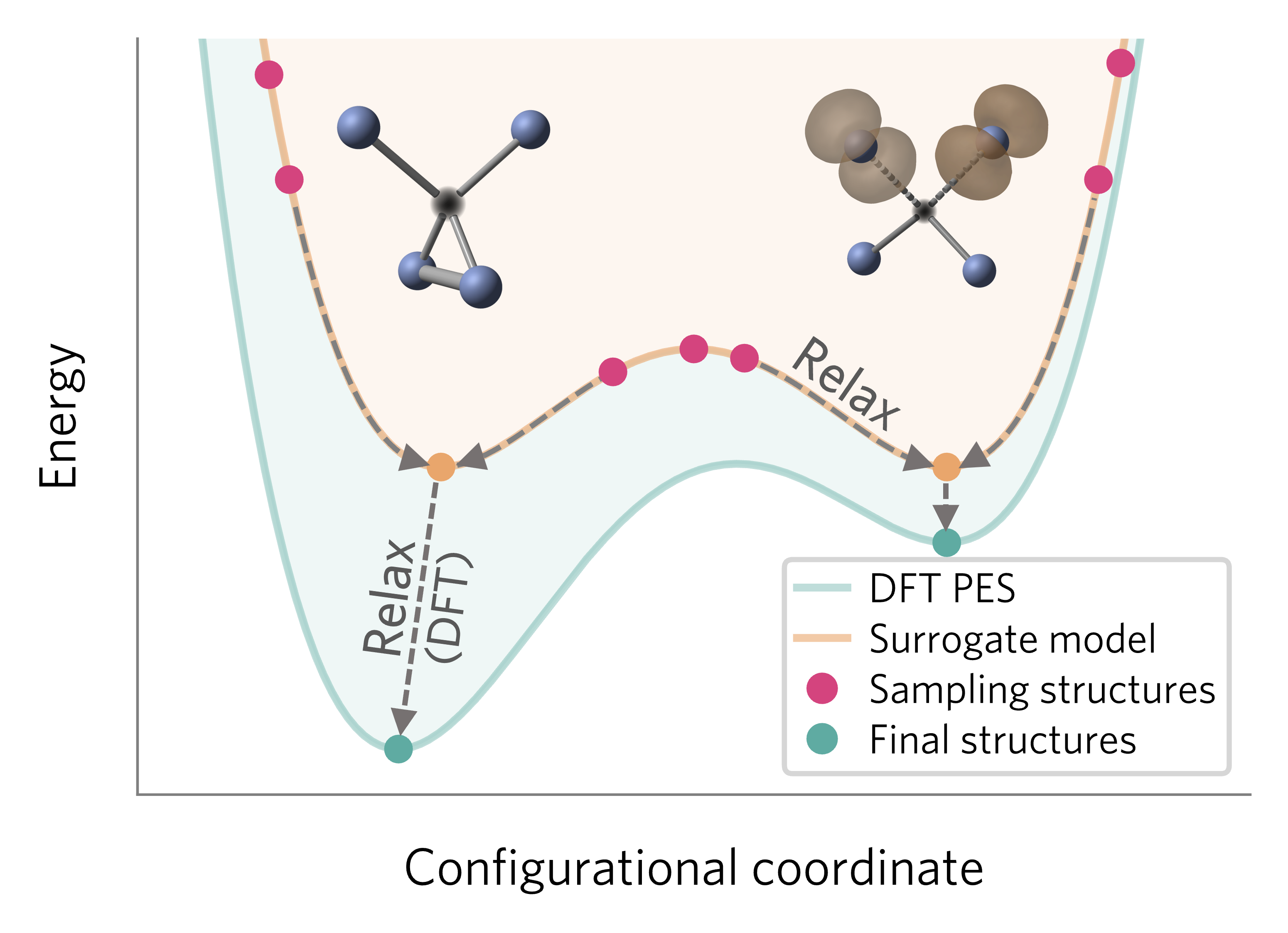
Figure 1: Schematic of a machine-learning surrogate model used to accelerate defect structure searching. The computationally efficient model learns the plausible defect reconstructions (local minima in the potential energy surface) and thus reduces the number of candidate structures relaxed with expensive first-principles density functional theory (DFT) calculations.

II Results

To assess the ability of a surrogate model to learn defect reconstructions, we will focus on one of the most common — and often strongest in terms of energy-lowering — reconstruction motifs: dimerisation[41, 49, 50, 51, 52, 53, 54, 55, 56, 57, 58, 59, 60, 61, 62, 63, 64, 51, 65, 66, 67, 68, 69, 70, 71, 54] . While cation dimerisation has been reported in several hosts (AgCl/Br, CuInSe2, CuGaSe2, ZnS/Se, CdTe, $\rm Sb_{2}S/Se_{3}$, CH3NH3PbI3, CsPbBr3, (CH3NH3)3Pb2I7, CH3NH3SnI3)[41, 49, 50, 51, 52], anion dimers are more common and will be the focus of our study.

To target dimerisation, we consider cation vacancies in low-symmetry metal sulfides/selenides, where their covalent character and soft structures favour dimer formation[41, 42, 54]. Our first-principles dataset spans 50 hosts (exemplified in 2a) and 132 neutral cation vacancies, covering 25 elements (3b) and 6 space groups. The configurational landscape of each vacancy was explored with the ShakeNBreak method[75, 41] by applying 15 chemically-guided distortions to the unperturbed defect structure, followed by geometry optimisation with DFT (IV) – resulting in a diverse set of trajectories for each defect and the dataset shown in 2c.

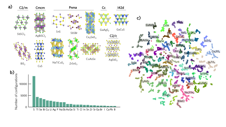
Figure 2: Distribution of the defect dataset generated with first-principles calculations. a) Example host structures and their respective space groups. b) Number of configurations containing each element. c) Two-dimensional projection of structural similarity for defect configurations. Each configuration is represented with the feature vector generated by the M3GNet model[76, 77] (trained on the bulk formation energies of the Materials Project database) and the vector dimensions are reduced using t-distributed stochastic neighbour embedding (t-SNE)[78, 79]. The defect configurations are coloured by their host composition (with similar colours indicating compositions with similar MEGNet[80] feature vectors), showing that related chemical systems cluster near each other. For clarity, in (b) and (c) 10 evenly spaced steps are selected from each relaxation trajectory.

II.1 Defect reconstructions

By analysing our first-principles dataset, we find that 29.9% of the neutral defects undergo symmetry-breaking reconstructions missed by both the standard modelling approach but also when applying a rattle distortion (with energy differences between the identified ground state and the relaxed ideal configuration greater than $0.5\text{\,}\mathrm{e}\mathrm{V}$; S1, S1). Rattle distortions (i.e. randomised displacements) have been used in recent studies[37] as the prevalence of defect reconstructions have become more recognised. While rattling helps to break the symmetry of the initial defect configuration and escape PES saddle points, it often fails to identify reconstructions with significant energy barriers (i.e. bond formation), highlighting the need for structure searching.

The identified reconstructions are driven by anion–anion bond formation, with the number of new bonds determined by the number of valence electrons lost upon defect formation (S2). In general, energy-lowering structural reconstructions at defects tend to be driven by the localisation of excess charge introduced by the defect formation, through various bonding (re-)arrangements. Here, excess charge refers to the change in valence electrons available for bonding, and in fact is the chemical guiding principle used in ShakeNBreak to target likely distortion pathways. Defects resulting in one hole (e.g. V${}_{\text{Li}}$ in Li4SnS4) can easily accommodate the missing charge without strong reconstructions, while defects with two or more holes (e.g. V${}_{\text{Bi}}$ in BiSI) tend to form anion dimers or trimers, as shown in 3b. As a result, anion–anion bonds are more favourable for more positive defect charge states, and can stabilise unexpected defect oxidation states, as observed previously for V${}_{\text{Sb}}$⁺¹ in $\rm Sb_{2}(S/Se)_{3}$[41, 42] and O${}_{\text{i}}$^+1,+2 in several metal oxides[41, 56, 53].

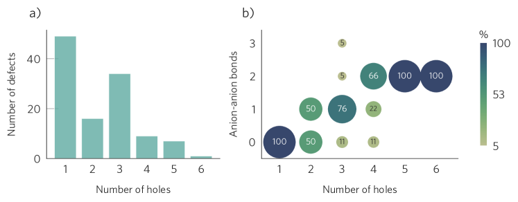
Figure 3: Analysis of the point defect dataset. a) Distribution of number of holes produced upon defect formation. b) Correlation between the number of anion–anion bonds formed and the number of holes created per defect. The label, colour, and size of the circles indicate the percentage of defects with that number of anion–anion bonds for defects for a given number of holes created.

There are some exceptions to this trend, where systems are able to accommodate three or more holes without undergoing strong reconstructions. One example is hosts with d/f metals that adopt multiple stable oxidation states (e.g. Fe, Co, Cu), which can accommodate a hole by adopting a higher oxidation state[8]. To verify this trend, we compared two isostructural $\rm A^{III}B^{I}S_{2}$ systems which only differ in the identity of the B cation: V${}_{\text{Ga}}$⁰ in $\rm Ga{\bf Cu}S_{2}$ and $\rm Ga{\bf Ag}S_{2}$; and V${}_{\text{In}}$⁰ in $\rm In{\bf Cu}S_{2}$ and $\rm In{\bf Ag}S_{2}$ (S3). In $\rm(Ga/In){\bf Ag}S_{2}$, two of the holes localise in a S–S bond formed by the vacancy nearest neighbours (NN), while the third hole is split between the remaining two NNs. In contrast, in $\rm(Ga/In){\bf Cu}S_{2}$, no dimer forms since three holes are localised in three of the vacancy NNs and five of the Cu ions closer to the vacancy — with these Cu ions showing shorter Cu–S bonds. The different behaviour of Cu and Ag can be rationalised by considering their second ionisation energies (I2(Cu): 20.3 eV, I2(Ag): 21.5 eV)[81], where the low I2 (and thus higher d states) of Cu(I) favours cation oxidation, while the higher I2 of Ag(I) results in a sulfur dimer accommodating two of the holes.

In addition to systems with d/f elements, defects with nearby anion–anion bonds can localise the positive charge in these bonds and thus avoid forming new ones. This behaviour is exemplified by RhSe2, where the two symmetry-inequivalent Rh vacancies show different reconstructions. The first vacancy site is surrounded by four Se–Se bonds (S4b), and thus can accommodate the four holes by depopulating the anti-bonding orbitals of these bonds. In contrast, the second site has only one Se–Se bond neighbouring the vacancy (S4c), and thus has to form an additional Se dimer to accommodate the positive charge.

Beyond chalcogenide dimers, other rearrangements to accommodate positive charge involve chalco-halide (e.g. S–Cl formed by V${}_{\text{Bi}}$⁰ in AgBiSCl2) and halide-halide bond formation (e.g. Cl dimers formed by V${}_{\text{Sb}}$⁰ in SbSCl9) (S5). Here we note that the zero-dimensional character of SbSCl9 enables this defect to undergo strong distortions forming two Cl dimers (S5). Overall, we highlight the common reconstruction motifs exhibited by different defects in various host structures (S2), facilitating the requisite diversity for a model to learn the plausible reconstructions for a group of related defects.

II.2 Model training

To develop a model that can be applied for defect structure searching in unseen compositions, we first split our dataset by composition into training, validation and test sets (S6), amounting to 68%, 5% and 27% of defects, respectively. The validation set is then augmented with 5% of the configurations selected for the systems in the training set, to ensure that the diversity of the training set is also included for validation. This results in training, validation and test sets of 11,955 (63%), 2,100 (11%), and 4,830 (26%) configurations, respectively, where configuration denotes a point defect structure with its associated energy, forces and stresses.

To sample the training data, we compared two approaches: i) a manual method where we sample 10 evenly spaced frames from each relaxation (MS) and ii) the Dimensionality-Reduced Encoded Clusters approach (DIRECT)[77], which aims to select a robust training set from a complex configurational space. Surprisingly, we find that, when using datasets of similar sizes, the MS approach performs better — with the DIRECT approach only outperforming MS when the final DIRECT dataset is larger than the MS one (S3). This is because the DIRECT approach mainly samples structures from the initial ionic steps (S9), which correspond to high distortions and thus lead to larger errors for the low energy structures (S10).

As a surrogate model, we aim for a method that takes an initial defect structure and outputs the energy and structure of the locally relaxed configuration. Machine-learning force fields are ideal for this task since they can map regions of the potential energy surface (PES) by learning the energies, forces, and, optionally stresses of a set of training structures. Specifically, we focus on universal graph-based MLFFs, which are trained on relaxation data from diverse databases of bulk crystals[76, 82, 83, 84], and thus already incorporate general chemical behaviour. Accordingly, we use a universal MLFF as a base model and fine-tune it with a training set of defect configurations. We have compared different model architectures (M3GNet[76], CHGNet[82] and MACE[85]), elemental reference energies, structure featurisation parameters (graph cutoffs, readout layers) and fine-tuning strategies, which are discussed in detail in the Supporting Information (SI) (Section S2). In addition, we compared a model trained on just defect structures, and both defect and bulk structures, with the second case improving performance (S10 and S12). From these benchmarks, the optimal model architecture and parameters were selected: a M3GNet model[76] with radial and 3-body cutoffs of $5\text{\,}\mathrm{\text{Å}}$ and $4\text{\,}\mathrm{\text{Å}}$, respectively, and the weighted atom readout function[76, 86] (further details in IV).

Overall, we note that the mean absolute errors for the absolute energies in the validation and test sets are significant ($\mathrm{MAE_{E,test}}=31.2~{}\mathrm{meV/atom}$, 1), but comparable to those obtained in MLFFs used for bulk structure searching of carbon ($\mathrm{MAE_{E,test}}=64.8~{}\mathrm{meV/atom}$)[87]. However, a more meaningful metric for our purpose is the error for the relative energies of each defect configuration relative to its ground state structure ($\mathrm{MAE_{E,rel,test}}=11.3~{}\mathrm{meV/atom}$). Further, we mostly care about the low-energy region of the potential energy surface, which can be measured by calculating the relative energy errors for configurations less than $\approx 5~{}\mathrm{eV}$ above the global minimum, resulting in MAEs of $3.6~{}\mathrm{meV/atom}\approx 0.29~{}\mathrm{eV}$ for an 80 atom supercell.

Beyond these metrics, we calculate the Spearman correlation coefficient ($\rho$) to measure how well the MLFF and DFT energies are monotonically related (i.e. if greater DFT energies correspond to greater MLFF energies[88]). While the value of $\rho$ for the test set is significantly lower than those obtained with MLFFs developed for bulk structure searching for a single composition (0.72 versus 0.98–0.999[88]), this was expected considering that our dataset spans a diverse range of compositions and a wide range of energies. While the errors are high, we note that this does not prevent the model from being used as a qualitative surrogate of the DFT PES for structure searching (i.e. identification of local minima), as previously observed for surface adsorbates[89, 90].

Table 1: Mean absolute errors (MAE) of the training, validation and test sets for energies (E), forces (F) and stresses (S). Distributions of the absolute errors are shown in S12.

Split	$\rm MAE_{E}$ (meV/atom)	$\rho$	$\rm MAE_{F}$ (meV/Å)	$\rm MAE_{S}$ (GPa)
Train	18.8	-	56.5	0.10
Val	27.0	0.86	93.4	0.13
Test	31.2	0.72	86.2	0.18

II.3 Model performance

To evaluate the model performance, we apply the trained model to a robust test set, which includes 13 unseen compositions and 32 defects (accounting for 26% and 26.5% of the total number of compositions and defects in our dataset, respectively; S6). For each defect, the MLFF is used to relax the 15 distorted structures generated with ShakeNBreak[75] to sample the defect PES. The MLFF-relaxed structures are then compared to identify the different local minima in the MLFF PES using the SOAP fingerprint[91] of the defect site. These local minima are then further relaxed with DFT. By comparing the ground state identified from the MLFF+DFT approach and full DFT search, we find the former to correctly identify the DFT ground state for 88% of test defects, while simultaneously reducing the number of DFT calculations required by 73% (2) and accelerating structure searching by a factor of 13 (S3.4). In addition, it identifies a more favourable structure than the ones found in the DFT search for V${}_{\text{Ge,9}}$ in TlGeS2, with an energy lowering of $0.5\text{\,}\mathrm{e}\mathrm{V}$ (S14).

Table 2: Performance of the trained model on the test set. The column “Local min. (DFT)” denotes the number of distinct structures identified in the DFT PES with ShakeNBreak. The column “Local min. (MLFF)” denotes the number of distinct structures identified in the MLFF PES, which are then further relaxed with DFT. “GS identified” shows whether the ground state structure located with DFT was also identified with the MLFF+DFT approach.

Hosts	Defect	Local min. (DFT)	Local min. (MLFF)	Symmetry broken	GS identified
BiSeBr	V${}_{\rm Bi_{0}}$	4	5	Yes	Yes
BiSeCl	V${}_{\rm Bi_{0}}$	3	4	Yes	Yes
BiSeI	V${}_{\rm Bi_{0}}$	6	3	Yes	No
CuAsS	V${}_{\rm As_{4}}$	2	4	No	Yes
CuAsS	V${}_{\rm Cu_{0}}$	2	1	No	Yes
CuS	V${}_{\rm Cu_{0}}$	1	3	No	Yes
CuS	V${}_{\rm Cu_{3}}$	3	2	No	Yes
CuSe	V${}_{\rm Cu_{0}}$	1	1	Yes	Yes
CuSe	V${}_{\rm Cu_{4}}$	2	1	Yes	Yes
Li4SnS4	V${}_{\rm Li_{0}}$	4	3	No	Yes
Li4SnS4	V${}_{\rm Li_{4}}$	3	3	No	Yes
Li4SnS4	V${}_{\rm Li_{8}}$	3	3	No	Yes
Li4SnS4	V${}_{\rm Sn_{16}}$	5	8	Yes	No
Ca2SnS4	V${}_{\rm Ca_{0}}$	3	3	Yes	No
Ca2SnS4	V${}_{\rm Ca_{4}}$	5	3	Yes	Yes
Ca2SnS4	V${}_{\rm Sn_{8}}$	2	3	Yes	Yes
Na2S5	V${}_{\rm Na_{0}}$	2	2	No	Yes
Na2S5	V${}_{\rm Na_{4}}$	2	3	No	Yes
Sb2S3	V${}_{\rm Sb_{1}}$	7	4	Yes	Yes
Sb2S3	V${}_{\rm Sb_{2}}$	9	7	Yes	Yes
Tl3PS4	V${}_{\rm Tl_{0}}$	2	3	No	Yes
Tl3PS4	V${}_{\rm Tl_{4}}$	5	3	No	Yes
Tl3PS4	V${}_{\rm P_{12}}$	7	5	Yes	Yes
Tl4Bi2S5	V${}_{\rm Tl_{0}}$	2	2	No	Yes
Tl4Bi2S5	V${}_{\rm Tl_{3}}$	1	1	No	Yes
Tl4Bi2S5	V${}_{\rm Tl_{11}}$	1	1	No	Yes
Tl4Bi2S5	V${}_{\rm Bi_{16}}$	3	2	Yes	Yes
Tl4Bi2S5	V${}_{\rm Bi_{20}}$	6	5	Yes	Yes
TlGeS2	V${}_{\rm Tl_{0}}$	5	1	Yes	No
TlGeS2	V${}_{\rm Ge_{8}}$	4	4	Yes	Yes
TlGeS2	V${}_{\rm Ge_{9}}$	5	4	Yes	Yes
Mean		4	3	0.51	0.88

The 12% of failed cases, where the MLFF ground state structure differed from the DFT one, mostly involve complex hosts. For instance, V${}_{\text{Sn}}$ in Li4SnS4 has a complex DFT energy surface, which traps most of the relaxations in very high energy basins (S18). PESs of similar complexity are displayed by the iso-structural systems that were included in the training set (Li4GeS4 and Li4TiS4; S18), which biases our training data to the high energy region of the PES for these compositions and thus hinders learning the low-energy region. Accordingly, the training data for these systems can be improved by reducing the magnitude of the distortion used by ShakeNBreak to generate their sampling structures; which would improve model performance. Other defects for which the surrogate model misses the most stable structure are V${}_{\text{Tl,0}}$ in TlGeS2 and V${}_{\text{Bi}}$ in BiSeI — yet in both cases the DFT and MLFF+DFT structures are very similar and differ by small energy differences (0.1 and 0.2 eV, respectively) (S16 and S15). In all failed cases, while the model misses the full DFT ground state, it still correctly predicts a favourable reconstruction, that lowers the energy compared to the relaxed ideal configuration.

Beyond identifying the correct ground state in the majority of cases, the model has indirectly learned the correlation between the number of holes and the number of formed dimers. For defects with 1 missing electron, the candidate structures generated by the surrogate model rarely contained anion–anion bonds; while for defects with more missing electrons, the model often identifies at least one local minima with a dimer.

The decreased performance observed for out-of-sample compositions less similar to the training set posed the question of what performance could be achieved if targeting a family of more related systems. To consider more similar host compositions, we select the chalcohalide systems from our dataset and split them composition-wise into training, validation and test sets as described in Section S4. After training the model on the training set and applying it to the unseen test defects (details on Section S4), we find that the model identifies the correct ground state for all test cases, and achieves lower mean absolute errors compared to the full model. This suggests that higher accuracy can be achieved when targeting more similar host structures, which is likely the case in most high-throughput defect studies.

Our current trained model is limited to neutral cation vacancies in metal sulphides/selenides. However, the approach can be extended to a different compositional space or defect type by first generating a custom training set through first-principles calculations and using it to fine-tune the universal bulk MLFF.

II.4 Application to alloys

Beyond high-throughput studies of many single-phase materials, the surrogate model can also be used to accelerate structure searching in alloys or disordered solids, which is computationally challenging due to the high number of local host compositions and inequivalent defects to consider[92]. The distinct local or site environments of a given defect can significantly affect its properties[34, 93, 94, 95, 96, 97, 98, 99, 100, 101, 102, 103, 35, 104], altering formation and migration energies by up to 1.5 eV[34, 94, 104, 101, 102, 35, 103]. Properly sampling various site environments is key to characterise the defect behaviour in such cases.

We consider the case of cadmium vacancies in the $\rm CdSe_{x}Te_{(1-x)}$ ($x=0,0.2,0.3,0.5,0.6,0.8,0.9,1$) pseudo-binary alloy. For each composition, a supercell is generated through random substitution of Te sites, and the Cd sites with a unique nearest neighbour chemical environment are considered (4a). The configurational landscape of each vacancy is explored with the ShakeNBreak method (14 sampling structures), using the relaxations from the pure compositions as the training and validation data while the mixed systems ($0<x<1$) are reserved as the test set.

After fine-tuning the surrogate model (MLFF) on the training configurations (details in IV), it is applied to all alloys to perform the structure searching calculations, allowing a more extensive sampling than for the DFT search (31 sampling structures). From the MLFF-relaxed structures, the unique configurations are selected for further relaxation with DFT and compared with the results from the DFT-only search. This comparison shows that the model successfully identifies the ground state for all defects, even in cases where the defects form Te-Se bonds not seen in the training set – which only included the Te-Te and Se-Se bonds formed by V${}_{\text{Cd}}$(CdTe) and V${}_{\text{Cd}}$(CdSe), respectively.

More significantly, for 70% of the defects, the model identifies a novel, more favourable ground state missed in the coarser DFT search (with a mean energy lowering of $-0.4\text{\,}\mathrm{e}\mathrm{V}$, Section S5). These reconstructions are driven by forming a more favourable anion–anion bond (4b) and missed in the DFT-only search due to the coarser sampling performed. This illustrates the advantage of the faster surrogate model to tackle defects with complex configurational landscapes, that require a more exhaustive exploration than a DFT-based search would allow, like alloys, compositionally disordered materials[105, 106, 107, 108], and low-symmetry or multinary systems with many degrees of freedom in their PES.

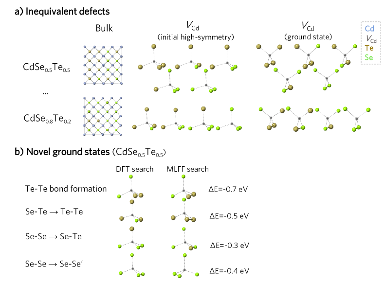
Figure 4: a) Inequivalent defect environments for two of the CdSe_xTe_1-x alloys ($x=0.5,0.8$). b) Examples of the ground state configurations only identified through the finer MLFF+DFT search. These reconstructions are driven by either forming a dimer (e.g. Te–Te bond formation), forming a more favourable anion–anion bond (Te–Te instead of Se–Te; Se–Te instead of Se–Se) or forming the same type of anion bond (Se-Se) but breaking weaker anion-cation bonds between the defect nearest neighbours and the defect next nearest neighbours.

III Conclusion

By building a dataset for defect structure searching, we have demonstrated the prevalence of defect reconstructions missed by the standard modelling approach – and thus the need to perform structure searching in high-throughput defect studies. To reduce the associated computational burden, we have developed a surrogate model by fine-tuning a universal machine-learning force field on defect configurations. By qualitatively learning the defect configurational landscapes, the trained model successfully predicts low-energy defect structures for unseen defects in unseen compositions, thereby reducing the number of DFT calculations by 73%. While our current model is limited to neutral cation vacancies in metal chalcogenides, the methodology can be applied to different defect types or compositional spaces. Accordingly, the approach could accelerate defect screening studies that target a range of dopants in a family of related host compounds. In addition, our openly-available dataset could be used to measure the out-of-distribution performance of universal MLFFs[109] by testing the ability to extrapolate from learned bulk motifs to defect environments.

Beyond accelerating structure searching in high-throughput studies, this approach is ideal for systems with a complex defect landscape, like alloys, disordered, or low-symmetry materials where their many inequivalent defects make it intractable to explicitly calculate all of them with accurate DFT methods. By using a surrogate model, we can consider a range of alloy compositions and all inequivalent defects, while performing a more exhaustive sampling of the PES — thereby identifying more favourable reconstructions missed in the (coarser) DFT-based search. Beyond (pseudo-)binary alloys, this approach could be extended to model more chemically complex systems, like high-entropy alloys, where the MLFF could be trained on defects of the constituent binary systems and applied to the ternary, quaternary, or high-entropy alloys.

A current limitation of this strategy is the handling of defects in distinct charge states, which have different energy landscapes and structural configurations (e.g. a defect in two different charge states can have a common local structure with different energies). The approach could handle the potential energy landscape for each charge state independently (e.g. training a separate model for defects in the -1 charge state). To consider different charge states simultaneously, the net charge state can be encoded as a graph global attribute[110]. However, a more descriptive encoding could be achieved by using fourth-generation MLFFs that include atomic charges[111]. Beyond accounting for the defect charge, another improvement could be MLFFs that are fine-tuned on-the-fly during geometry optimisations. As shown for surface absorbates[89, 90], this strategy would accelerate the defect geometry optimisation by skipping many ionic steps that are performed with the surrogate model. Overall, we note the promise of surrogate models to accelerate and increase the accuracy of defect modelling, whether this is by improving structure searching, accounting for metastable configurations[112, 113], enabling the calculation of defect formation entropies[110, 113], accelerating defect migration studies[114] or going beyond the dilute limit[108].

IV Methods

IV.1 High-throughput vacancies in chalcogenide hosts

Defect initialisation. The conventional supercell approach for modelling defects in periodic solids was used[115]. To reduce periodic image interactions, supercell dimensions of at least $10\text{\,}\mathrm{\text{Å}}$ in each direction[116] were employed. To explore the configurational landscape of each defect, we used the ShakeNBreak code[75], with a distortion increment of 0.1 and the default rattle standard deviation (10% of the nearest neighbour distance in the bulk supercell). This strategy results in 14 sampling structures. In addition to these, to ensure that dimerisation was properly sampled, we also generated a sampling structure where two defect neighbours were pushed towards each other with a separation of $2\text{\,}\mathrm{\text{Å}}$, resulting in a total of 15 initial configurations.

First-principles calculations. All reference calculations were performed with Density Functional Theory using the exchange-correlation functional HSE06[117] and the projector augmented wave method[118], as implemented in the Vienna Ab initio Simulation Package[119, 120]. Calculations for the pristine unit cells were performed using a plane wave energy cutoff of $585\text{\,}\mathrm{e}\mathrm{V}$ and sampling reciprocal space with a Monkhorst-Pack mesh of density 900 k-points/site. The convergence thresholds for the geometry optimisations were set to $10^{-6}$ eV and $10^{-5}$eV/Å for energy and forces, respectively. Defect relaxations were performed with the $\Gamma$-point approximation, which is accurate enough for defect structure searching[41], and with a plane wave energy cutoff of $350\text{\,}\mathrm{e}\mathrm{V}$. The energy and force thresholds for defect relaxations were set to $10^{-4}$ eV and $10^{-2}$ eV/Å, respectively. To automate the generation of input files, we designed a workflow using aiida[121, 122, 123], pymatgen[124, 125, 126], pymatgen-analysis-defects[127], ASE[128], doped[129] and ShakeNBreak[75]. This code is available from https://github.com/ireaml/defects_workflow.git. The datasets and trained models are available from the Zenodo repository with DOI 10.5281/zenodo.10514567.

Surrogate machine learning model. To generate the training and test set for the machine learning model, we processed the DFT defect relaxation data by removing unreasonably high-energy configurations (e.g. structures with positive energies), as they decreased model performance. After cleaning the data, 10 evenly-spaced ionic steps were selected from each relaxation. We used the M3GNet model[76], as implemented in Ref. 86, with radial and 3 body cutoffs of $5\text{\,}\mathrm{\text{Å}}$ and $4\text{\,}\mathrm{\text{Å}}$, respectively, and the weighted atom readout function. The loss function was defined as a combination of the mean squared errors for the energies, forces and stresses, with respective weights of 1, 1 and 0.1[76, 86]. For fine-tuning, the model was initialised with the weights from the trained bulk crystal model[86] and then trained on the defect training set (see S2.5 for further details). A batch size of 4 and an exponential learning rate scheduler with an initial rate of $5\times 10^{-4}$ were used. The model was trained on a Quadro RTX6000 GPU until the validation errors were converged (30 epochs, 5.3 hours) (S13).

Model application. MLFF geometry optimisation was performed with the FIRE algorithm[130], as implemented in the ASE package[128], until the mean force was lower than $10^{-5}$ eV/Å or the number of ionic steps exceeded 1500, which were found to be reasonable thresholds. After relaxing the sampling structures with the model, we identified the different local minima or configurations by calculating the cosine distance between the SOAP descriptor[91] for the defect site of each configuration, which was found to be an effective metric for identifying different defect motifs. The parameters used to generate the SOAP descriptor were: $r=5$ Å, $n_{max}=10,l_{max}=10,\sigma=1.0$ Å, for the local cutoff, number of radial basis functions, maximum degree of spherical harmonics, and the standard deviation of the Gaussian functions used to expand the atomic density, respectively.

IV.2 Application to the $\mathrm{CdSe_{x}Te_{(1-x)}}$ alloy

Data generation. To generate the supercells for the mixed compositions in $\rm CdSe_{x}Te_{(1-x)}$ ($x=0.2,0.3,0.5,0.6,0.8,0.9$), we used random substitution of Te sites with Se. For each supercell, we consider the Cd sites with a unique nearest neighbour chemical environment as vacancy sites, and generate the vacancy high-symmetry structures with pymatgen[124, 125, 126]. For the DFT-based exploration of the PES, we apply ShakeNBreak with default parameters, generating 14 sampling structures, which were relaxed with DFT as previously described.

Model training. To generate the dataset, we again processed the defect relaxation data by removing unreasonably high-energy configurations ($>15$ eV above the defect ground state configuration). As the training set, we used a combination of defect and bulk configurations: 45 evenly-spaced frames from the 14 relaxations of V${}_{\text{Cd}}$ in CdTe and CdSe, and 20 frames from the relaxations of each pristine system, resulting in a total of 1420 frames. For validation, we selected 5 unseen configurations from the 14 relaxations of V${}_{\text{Cd}}$ in CdTe and CdSe (total of 140 frames). The M3GNet surrogate model was trained with similar parameters as previously described and until the errors were converged (80 epochs, see S24).

Finer exploration of the PES. To perform a finer exploration of the PES with the surrogate model, we applied a set of bond distortions generated by ShakeNBreak (-0.6, -0.5, -0.4, -0.3, -0.2) to all unique pair combinations of nearest neighbours (e.g. for a V${}_{\text{Cd}}$ surrounded by two Te and two Se anions, Te(1), Te(2), Se(1) and Se(2), we considered the pairs Te(1)-Te(2), Te(1)-Se(1), Te(1)-Se(2), Te(2)-Se(1), Te(2)-Se(2), and Se(1)-Se(2)). By default, for a defect with two missing electrons like V${}_{\text{Cd}}$⁰ , ShakeNBreak only applies the bond distortions to the two atoms closest to the defect. This is typically a reliable approach for most pure systems, but can miss reconstructions for alloys with complex defect environments (e.g. V${}_{\text{Cd}}$ surrounded by a mix of Te and Se anions). The model application and analysis were performed as described in the previous section.

Declarations

Data & code availability. The code used to generate the defect dataset is available from https://github.com/ireaml/defects_workflow.git. The datasets and trained models are available from the Zenodo repository with DOI 10.5281/zenodo.10514567.

Acknowledgments. We thank David O. Scanlon for discussions on defect symmetry breaking. I.M.L. acknowledges Imperial College London for funding a President’s PhD scholarship. S.R.K. acknowledges the EPSRC Centre for Doctoral Training in the Advanced Characterisation of Materials (CDT-ACM)(EP/S023259/1) for funding a PhD studentship. A.M.G. is supported by EPSRC Fellowship EP/T033231/1. A. W. is supported by EPSRC project EP/X037754/1. We are grateful to the UK Materials and Molecular Modelling Hub for computational resources, which is partially funded by EPSRC (EP/P020194/1 and EP/T022213/1). This work used the ARCHER2 UK National Supercomputing Service (https://www.archer2.ac.uk) via our membership of the UK’s HEC Materials Chemistry Consortium, which is funded by EPSRC (EP/L000202). We acknowledge the Imperial College London’s High Performance Computing services for computational resources.

Author contributions. Conceptualisation & Project Administration: All authors. Investigation and methodology: I.M.-L. Supervision: S.R.K., A.M.G., A.W. Writing - original draft: I.M.-L. Writing - review & editing: All authors. Resources and funding acquisition: A.M.G., A.W. These author contributions are defined according to the CRediT contributor roles taxonomy.

Competing interests. The authors declare no competing interests.

Supplementary Information for ‘Machine-learning structural reconstructions for accelerated point defect calculations’

S1 Dataset analysis

Table S1: Percentage of defects that lead to energy-lowering reconstructions (compared to a typical unperturbed relaxation) higher than the specified energy threshold. The column ‘Reconstructions found with rattling’ indicates the percentage of reconstructions identified if we only apply randomised distortions to the unperturbed, ideal defect structure (i.e. no bond distortions), demonstrating the need for proper structure searching.

Threshold (eV)	Significant reconstructions (%)	Reconstructions found with rattling (%)
-0.05	40.3	3.7
-0.10	33.6	0
-0.50	29.9	0
-1.00	20.9	0
-2.00	6.7	0

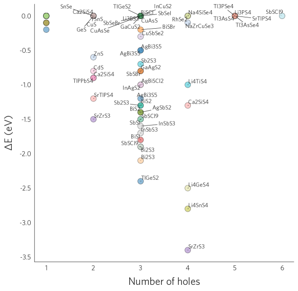
Figure S1: Energy difference between the ground state structure identified with ShakeNBreak and the final structure obtained by relaxing the ideal, high-symmetry defect structure for cation vacancies across each chalcogenide. Note that all defects with more than 3 missing electrons form dimer reconstructions, but some appear with $\Delta E=0~{}\mathrm{eV}$ since the ground state structure is already identified from the high-symmetry relaxation.

S1.1 Defect reconstructions

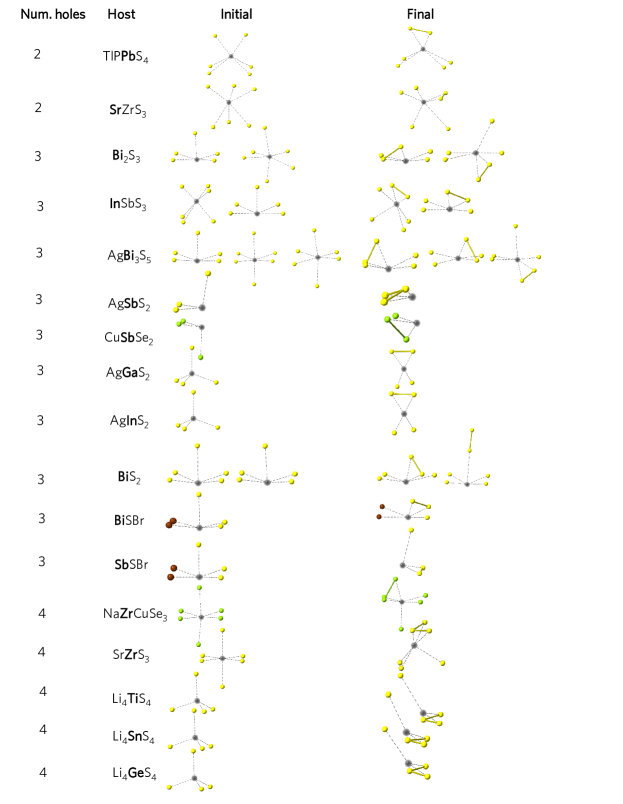
Figure S2: Illustration of some of the reconstructions identified, showing the similar motifs undergone by different hosts. The initial (high-symmetry) and the ground state structures are shown. The defect element is shown in bold in the host composition.

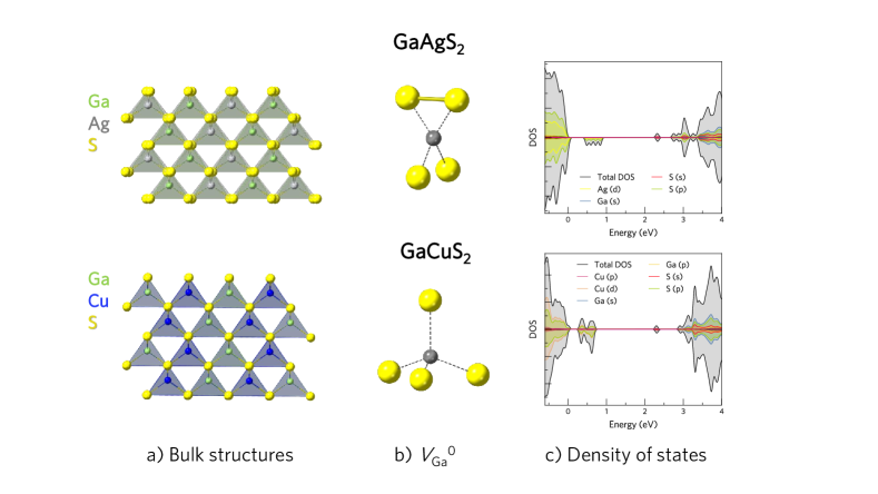
Figure S3: Reconstructions undergone by V${}_{\text{Ga}}$⁰ in GaAgS2 and GaCuS2. a) Bulk structures for GaAgS2 (top) and GaCuS2 (bottom). b) V${}_{\text{Ga}}$⁰ , showing the dimerisation undergone in GaAgS2 while in GaCuS2 V${}_{\text{Ga}}$⁰ maintains the ideal tetrahedral coordination. Similar behaviour is observed for V${}_{\text{In}}$⁰ in InAg/CuS2. c) Density of states for V${}_{\text{Ga}}$⁰ , showing the localised defect states within the gap.

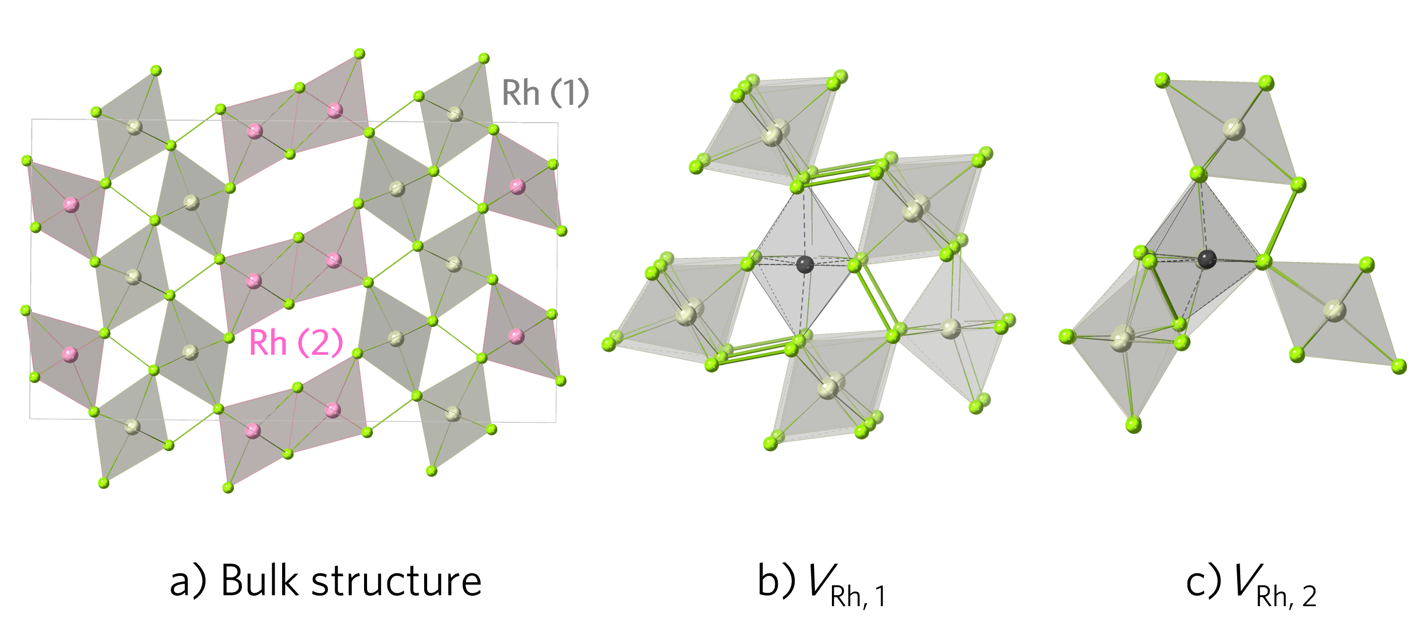
Figure S4: Reconstructions undergone by the symmetry inequivalent Rh vacancies in RhSe2. a) Bulk structure showing the two symmetry inequivalent Rh sites, in grey (Rh(1)) and pink (Rh(2)). b) V${}_{\text{Rh,1}}$ does not form a Se dimer since the holes can localise in the Se-Se bonds already neighbouring this site. c) V${}_{\text{Rh,2}}$ forms an additional Se-Se bond as it lacks enough neighbouring Se-Se bonds to localise the four holes.

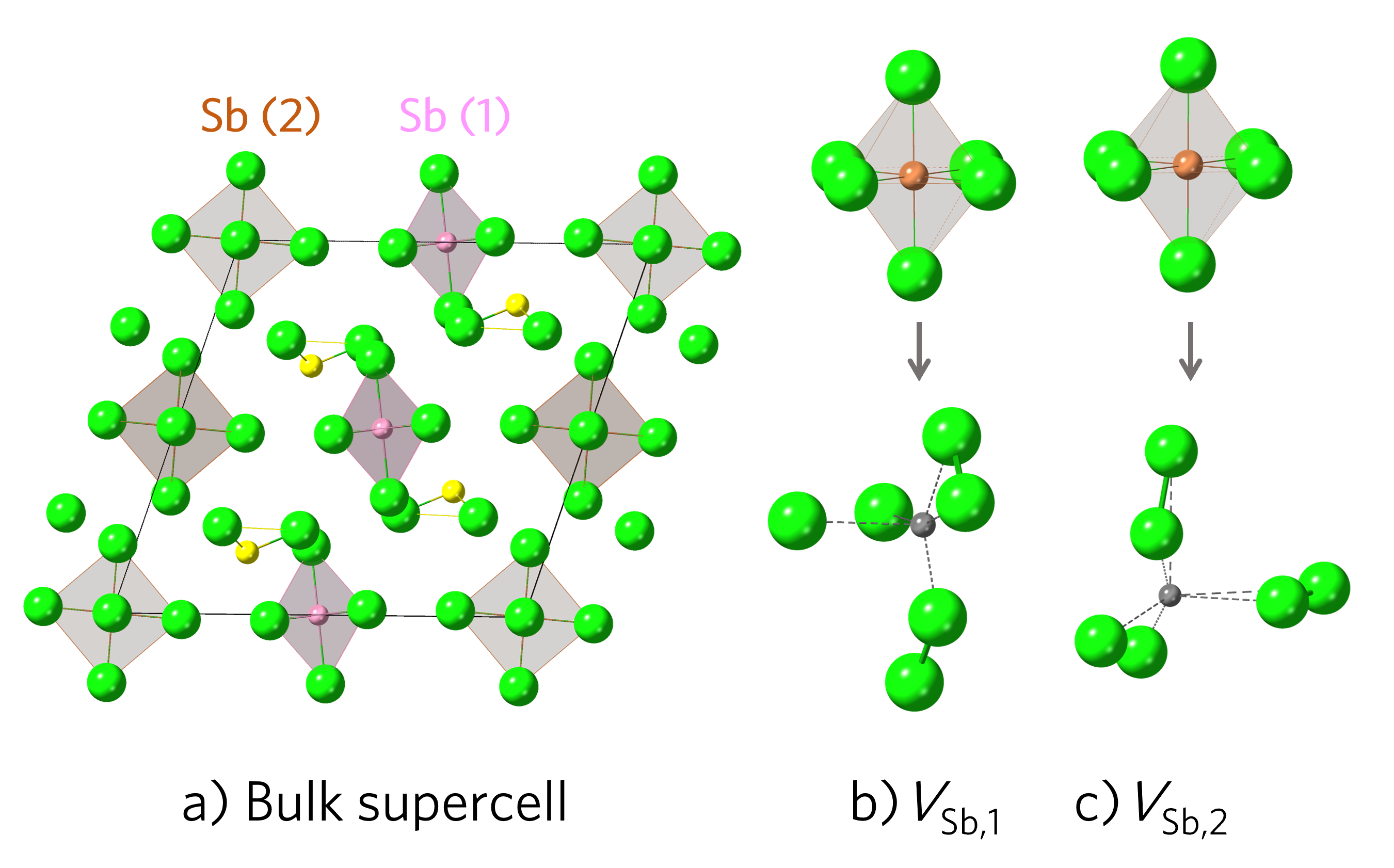
Figure S5: Reconstructions undergone by the symmetry inequivalent Sb vacancies in SbSCl9. a) Bulk structure showing the two symmetry inequivalent Sb sites, in pink (Sb(1)) and brown (Sb(2)). b, c) V${}_{\text{Sb,1}}$ and V${}_{\text{Sb,2}}$ forming two Cl-Cl dimers.

S2 Model training

In this section, we compare different training strategies and parameters. We note that errors are higher than in the final model since here most of the parameters were set to default values except for the parameter being benchmarked. Further, in these experiments, the validation set only contained unseen compositions (and not unseen configurations from compositions included in the training set).

S2.1 Splits

The dataset was first split by composition into training, composition, and test sets, as shown in S6.

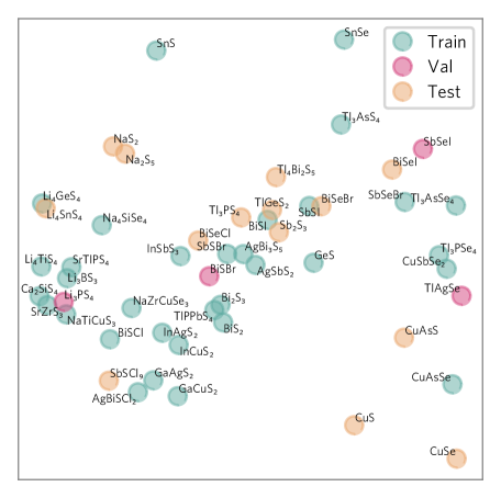
Figure S6: Plot of the first two principal components of the feature space for the pristine structures, showing the division into training, validation, and test sets. We note that the validation set was then augmented with some configurations from the compositions in the training set. The structures were encoded with the 128-element vector outputs from the M3GNet model trained on the formation energies of bulk materials in the Materials Project database, as done in Ref. 77.

S2.2 Reference energies

Before fitting most MLFFs, it is common to subtract the reference elemental energies from the total energies to improve training stability[76]. In M3GNet[76], the reference elemental energies can be calculated from the training or other user-specified data using linear regression[76]. To compare the effect of the reference elemental energies, we considered three different approaches to calculate them: i) energies of the isolated atoms, ii) linear regression to the bulk energies, and iii) linear regression to the energies of all training defect structures. As expected, the last case decreases performance since the regressed reference energies include defect formation contributions. On the other hand, when the reference elemental energies are calculated from the bulk systems, these constitute a robust reference that simplifies learning the energies of different defect structures.

Table S2: Comparison of model performance depending on the elemental reference energies used. The same training and validation data and training parameters are used for all cases and the performance is measured with the mean absolute errors of the energies, forces, and stresses.

Method	$\rm Loss_{val}$	$\rm E_{val}$ (meV/atom)	$\rm F_{val}$ (meV/Å)	$\rm S_{val}$ (GPa)	$\rm E_{train}$ (meV/atom)	$\rm F_{train}$ (meV/Å)	$\rm S_{train}$ (GPa)
Bulk	0.22	41.8	153.8	0.22	50.50	118.0	0.19
Isolated atoms	0.31	72.4	191.6	0.43	134.5	154.3	0.30
Defect	0.34	130.3	179.3	0.34	109.6	158.2	0.28

S2.3 Sampling methods

To investigate how to best sample configurations from the relaxation trajectories to generate the training set we compared two approaches: i) a manual method where we sample 10 evenly spaced frames from each relaxation (MS) and ii) the Dimensionality-Reduced Encoded Clusters approach (DIRECT)[77], which aims to select a robust training set from a complex configurational space (S7). This comparison was performed without including configurations of the bulk (pristine) host structures. After generating the different training sets, four M3GNet models[76] with default parameters were trained and evaluated. As shown in S3, when using training sets of similar sizes, the manual model performs better. This results from the DIRECT approach mostly sampling highly distorted configurations from the initial ionic steps (S9), hindering the learning of the low-energy region of the potential energy surface (PES).

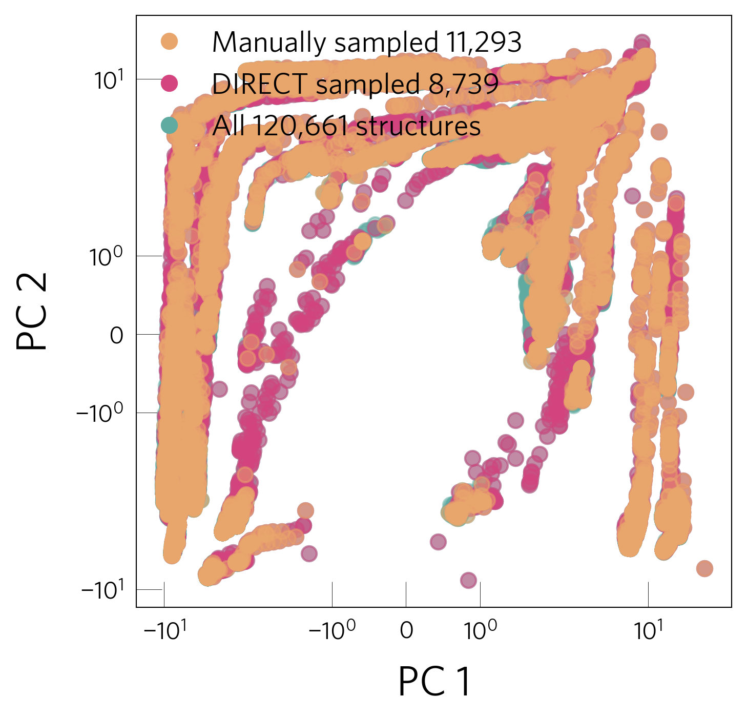
(a) DIRECT and manual coverage

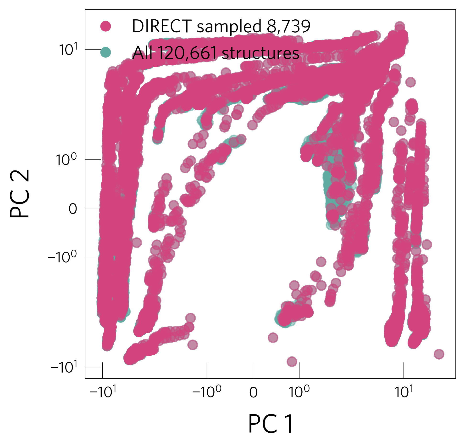
(b) DIRECT only (for clarity)

Figure S7: Sampling coverage of manual (orange) and DIRECT sampling (pink) of the full dataset (green), illustrating that the DIRECT approach covers better the configurational landscape. For the DIRECT method, we considered the parameters t=0.02, n=4000, k=20, but similar behaviour is observed for the other cases of S3. Note that the dataset is only plotted along two dimensions (see S8). The structures were encoded with the 128-element vector outputs from the M3GNet model trained on the formation energies of bulk materials in the Materials Project database[77]. For further details of the method used to featurise structures, dimensionality reduction, clustering, and stratified sampling see the original publication of Qi et al[77].

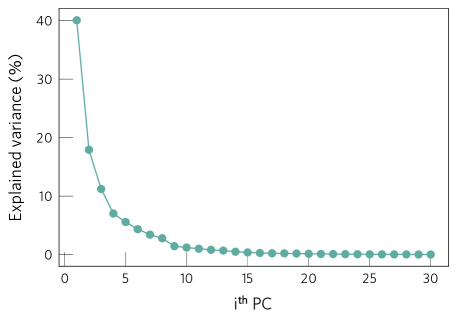
Figure S8: Explained variance versus the number of PCA dimensions. PCA was used to reduce the dimensions of the feature vector used to describe the defect configurations (see Ref. 77 for details).

Table S3: Comparison of the mean absolute errors in the validation and training sets obtained with the different methods of sampling the training data. The same validation data and training parameters are used for all cases. The column ‘Params.’ lists the sampling parameters used with the BIRCH clustering method, as detailed in Ref. 77.

Method	Size	Params. (t, n, k)	$\rm Loss_{val}$	$\rm E_{val}$ (meV/atom)	$\rm F_{val}$ (meV/Å)	$\rm S_{val}$ (GPa)	$\rm E_{train}$ (meV/atom)	$\rm F_{train}$ (meV/Å)	$\rm S_{train}$ (GPa)
Direct	21149	0.02, 4000, 20	0.20	28.6	148.6	0.19	38.1	147.6	0.19
Manual	11335	-	0.22	51.4	146.7	0.26	62.0	123.3	0.23
Direct	8705	0.1, 1000, 20	0.25	47.0	174.7	0.33	42.2	177.3	0.23
Direct	13144	0.03, 2000, 20	0.28	93.4	165.3	0.26	54.9	192.3	0.26

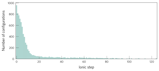
Figure S9: Distribution of DIRECT (t=0.02, n=4000, k=20) sampled configurations, showing that structures are mainly selected from the initial ionic steps, which correspond to highly distorted structures.

Figure S10: Distribution of the energy (a, b, c) and force (d, e) absolute errors for the test set. The MS sampling results in lower errors for the low-energy structures while the DIRECT approach leads to higher errors for these structures. a) Distribution of absolute energy errors versus the absolute DFT energy for all test compositions. b) Same as (a) but with the DFT energies normalised for each defect, so that energies of different defects/compositions are comparable. c) Same as (b) but removing very high energy configurations to aid visualisation. d) Distribution of absolute force errors versus the magnitude of the DFT forces. Same as (c) but removing configurations with very high forces. We note that the configurations with very high errors correspond to the most challenging compositions (more different from the training set, like the quasi-one-dimensional system SbSCl9).

S2.4 Model architecture

To compare different model architectures, we trained from scratch (i.e. initialising the weights with random values) three models: M3GNet[76], MACE[85] and CHGNet[82]. Again, for simplicity, this comparison was performed with default parameters for each model. The same training, validation, and test sets were used to compare the different models. The worse performance of CHGNet compared to the other models seems to arise from two reasons: i) the smaller value of the 3-body cutoff that is used by default ($3\text{\,}\mathrm{\text{Å}}$ compared to $4\text{\,}\mathrm{\text{Å}}$ in M3GNet) and ii) its default readout or pooling layer, which involves an average function (with the attention layer performing better). Regarding M3GNet and MACE, MACE seems to perform better on the test set. However, due to the lack of a pre-trained MACE universal model at the time when this comparison was performed, we decided to use M3GNet. However, with the now available MACE universal model, we expect the MACE architecture to perform better.

Table S4: Comparison of validation and test mean absolute errors for different models (M3GNet, CHGNet, MACE). For the test set, the Spearman coefficient for the energies ($\rho$) is also shown. The default parameters of each model were used and the models were trained from scratch (without fine-tuning/pretraining). In all cases, the training data included energies, forces and stresses.

Model	$\rm E_{val}$ (meV/atom)	$\rm F_{val}$ (meV/Å)	$\rm E_{test}$ (meV/atom)	$\rm F_{test}$ (meV/Å)	$\rho_{\rm test}$
M3GNet	45.8	143.1	129.2	263.0	0.44
MACE	47.8	173.9	153.7	187.8	0.66
CHGNet	192.3	351.4	376.0	333.8	0.37

S2.5 Training parameters for M3GNet model

To determine the best training parameters for the M3GNet model, we performed several benchmarks by comparing training and validation errors. From these comparisons, we determined the best learning rate, radial and 3-body cutoffs and readout function. We note that these comparisons were performed on the training and validation errors, rather than test ones, as they were intended as quick benchmarks to determine appropriate training parameters. Further, note that the errors are higher than for the final model since the default values were used for the parameters not being tested in each experiment.

S2.5.1 Learning rate

Table S5: Comparison of validation mean absolute errors for different learning rates and learning rate schedulers. ‘Constant’ denotes using a constant learning rate. When a scheduler is used, the initial learning rate is given in parentheses. Rows are ordered by ascending validation loss. The same training data (manual sampling) and training parameters were used for all experiments.

Method	$\rm Loss_{val}$	$\rm E_{val}$ (meV/atom)	$\rm F_{val}$ (meV/Å)	$\rm S_{val}$ (GPa)	$\rm E_{train}$ (meV/atom)	$\rm F_{train}$ (meV/Å)	$\rm S_{train}$ (GPa)
Exp. scheduler ($5\cdot 10^{-4}$)	0.19	35.7	128.0	0.22	30.9	93.0	0.16
Cos. scheduler ($10^{-3}$)	0.20	41.8	135.4	0.26	32.2	106.8	0.17
Constant ($5\cdot 10^{-4}$)	0.21	45.0	142.6	0.19	34.1	96.2	0.16
Constant ($10^{-3}$)	0.21	45.8	143.1	0.19	36.7	97.9	0.17
Exp. scheduler ($10^{-3}$)	0.21	25.8	152.9	0.36	21.8	85.70	0.12
Constant ($10^{-4}$)	0.24	58.8	152.1	0.29	56.7	131.4	0.22
Time. scheduler ($10^{-3}$)	0.25	64.3	152.0	0.31	35.2	101.4	0.16
Constant ($10^{-5}$)	0.29	70.9	191.2	0.32	84.8	174.1	0.41

S2.5.2 Structure featurisation

We performed benchmarks to identify the optimal values for the radial and 3-body cutoff and the optimal function for the pooling layer. As shown in S6, S7, S8, we found a 3-body cutoff of $4\text{\,}\mathrm{\text{Å}}$, a radial cutoff of $5\text{\,}\mathrm{\text{Å}}$, and the weighted atom layer from the M3GNet model to work best.

Table S6: Comparison of cutoff values for the 3-body radius in the M3GNet model. Mean absolute errors for energies, forces, and stresses for the training and validation sets. Rows are ordered by ascending validation loss.

cutoff (Å)	$\rm Loss_{val}$	$\rm E_{val}$ (meV/atom)	$\rm F_{val}$ (meV/Å)	$\rm S_{val}$ (GPa)	$\rm E_{train}$ (meV/atom)	$\rm F_{train}$ (meV/Å)	$\rm S_{train}$ (GPa)
4	0.19	35.7	128.0	0.22	30.9	93.0	0.16
3	0.26	59.2	164.9	0.32	50.6	123.5	0.20

Table S7: Performance comparison for different radial cutoffs in the M3GNet model. Mean absolute errors for energies, forces, and stresses for the training and validation sets. Rows are ordered by ascending validation loss.

cutoff (Å)	$\rm Loss_{val}$	$\rm E_{val}$ (meV/atom)	$\rm F_{val}$ (meV/Å)	$\rm S_{val}$ (GPa)	$\rm E_{train}$ (meV/atom)	$\rm F_{train}$ (meV/Å)	$\rm S_{train}$ (GPa)
5	0.19	35.7	128.0	0.22	30.9	93.0	0.16
4.5	0.22	40.1	142.0	0.34	35.1	97.4	0.16
5.5	0.23	57.1	140.7	0.31	46.8	114.4	0.20
6	0.23	73.9	133.0	0.22	45.9	103.4	0.18

Table S8: Performance comparison for different readout functions in the M3GNet model. Mean absolute errors for energies, forces, and stresses for the training and validation sets. Rows are ordered by ascending validation loss.

Readout	$\rm Loss_{val}$	$\rm E_{val}$ (meV/atom)	$\rm F_{val}$ (meV/Å)	$\rm S_{val}$ (GPa)	$\rm E_{train}$ (meV/atom)	$\rm F_{train}$ (meV/Å)	$\rm S_{train}$ (GPa)
Weighted atom	0.19	35.7	128.0	0.22	30.9	93.0	0.16
Reduce readout	0.23	54.6	143.1	0.30	65.0	135.1	0.24
Set2Set	0.26	57.7	163.9	0.39	44.3	130.9	0.2

S2.5.3 Fine-tuning

To assess the effect of fine-tuning the model from a model trained on the bulk relaxations of the Materials Project database, we compared the performance of four different models: training from scratch (i.e. initialising the weights with random values), or fine-tuning the bulk model (either training all layers or only the last final layers). When comparing their performance on the validation set, we found that fine-tuning the bulk model and training all layers resulted in the best performance, with the main benefit observed for the forces.

Table S9: Performance comparison between different training strategies: training from scratch (initialising the weights with random values), or fine-tuning the model previously trained on the Materials Project dataset of bulk structures[76] (with either re-training all layers (all), only the last two layers (2) or only the last layer (1)). The performance is measured with the mean absolute errors in the validation and training sets.

Training	$\rm Loss_{val}$	$\rm E_{val}$ (meV/atom)	$\rm F_{val}$ (meV/Å)	$\rm S_{val}$ (GPa)	$\rm E_{train}$ (meV/atom)	$\rm F_{train}$ (meV/Å)	$\rm S_{train}$ (GPa)
Fine-tuning (all)	0.157	42.6	101.1	0.1	18.7	68.1	0.1
Fine-tuning (1)	0.176	37.6	118.8	0.2	18.3	76.0	0.1
Fine-tuning (2)	0.183	36.5	104.9	0.4	15.2	55.4	0.1
From scratch	0.187	46.4	121.5	0.2	27.7	86.1	0.1

S2.6 Adding bulk data to enhance defect dataset

To test whether adding data for pristine systems would improve model performance, we trained two models: one on just the defect dataset (using MS sampling) and another model using the same defect dataset but combined with a small fraction of pristine configurations for the same compositions (5 evenly spaced frames from the relaxation of each pristine structure). As shown in S10, adding bulk data reduces the mean absolute errors for the energies and the forces of the test configurations. By analysing the error distributions in S11, we see that the main benefit of including bulk data is to reduce the errors for systems that are difficult due to their higher structural difference from the training set (i.e. including bulk data results in lower MAE and RMSE when considering all test systems (S11.a) but in a higher MAE and RMSE when not considering the harder compositions (S11.b)).

Table S10: Performance comparison when adding bulk (pristine) configurations to the training dataset. Mean absolute errors (MAE) and root mean square errors (RMSE) for the (defect) test set when only training on defect data and when training on both defect and bulk data.

Dataset	$\rm MAE_{E}$ (meV/atom)	$\rm RMSE_{E}$ (meV/atom)	$\rho$	$\rm MAE_{F}$ (meV/Å)	$\rm RMSE_{F}$ (meV/Å)	$\rm MAE_{S}$ (GPa)	$\rm RMSE_{S}$ (GPa)
Defect + Bulk	27.3	39.4	0.70	86.8	1943.5	0.19	0.54
Defect only	63.4	119.5	0.63	135.0	1139.6	0.34	0.70

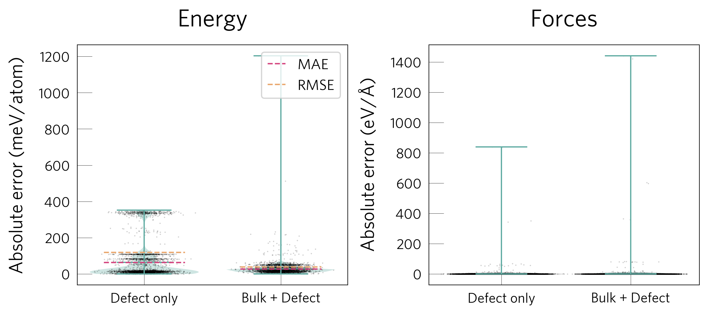
(a) All test systems

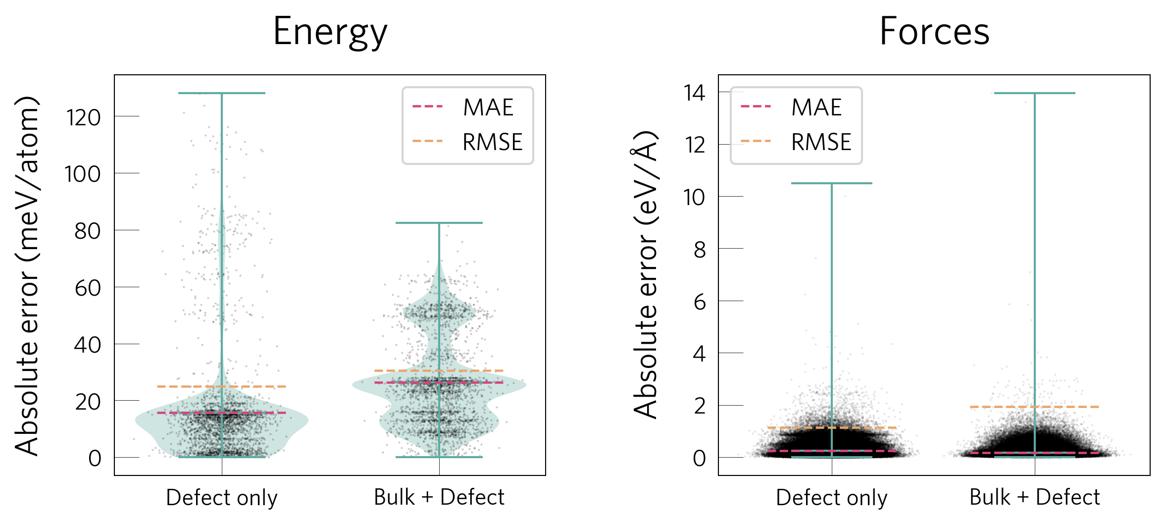
(b) Removing difficult compositions from test set

Figure S11: Violin plots[131] and error metrics for energies and forces on the test set. a) When considering all test systems. b) When filtering out the systems that are hard to learn due to high structural differences to the training set (SbSCl9, NaS2 and CuS).

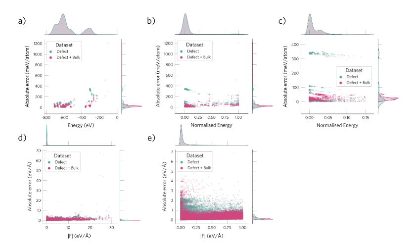
Figure S12: Distribution of absolute errors for energies (a, b, c) and forces (c, d) when training on only defect data (green) and both defect and bulk data (pink). a) Distribution of absolute energy errors versus the absolute DFT energy for all test compositions. b) Same as (a) but with the DFT energies normalised for each defect, so that energies of different defects/compositions are comparable. c) Same as (b) but removing very high energy configurations, illustrating how adding bulk data reduces the errors of many low-energy structures. d) Distribution of absolute force errors versus the magnitude of the DFT forces. Same as (c) but removing configurations with very high forces, illustrating how adding bulk data reduces the errors for low force configurations.

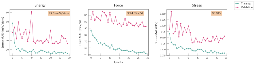
Figure S13: Evolution of training and validation errors with epoch number. The validation errors obtained for the epoch with the lowest validation loss are shown at the top right of each subplot.

S3 Model performance

S3.1 Metrics

Table S11: Performance of the fine-tuned surrogate model on the test set. Mean absolute errors (MAE, in eV and eV/atom) when predicting the relative energies of the low-energy configurations of a defect (i.e. structures that are less than $5\text{\,}\mathrm{e}\mathrm{V}$ above the defect ground state configuration).

	MAE (eV)	MAE (meV/atom)
Li4SnS4	1.6	11.2
BiSeBr	0.7	1.4
TlGeS2	0.6	0.7
Tl3PS4	0.4	1.6
SbSCl9	0.2	9.6
Tl4Bi2S5	0.2	5.0
BiSeCl	0.2	1.2
CuS	0.2	1.2
Na2S5	0.2	2.9
CuAsS	0.1	0.9
NaS2	0.1	2.8
CuSe	0.1	1.9

S3.2 New ground states: TlGeS2

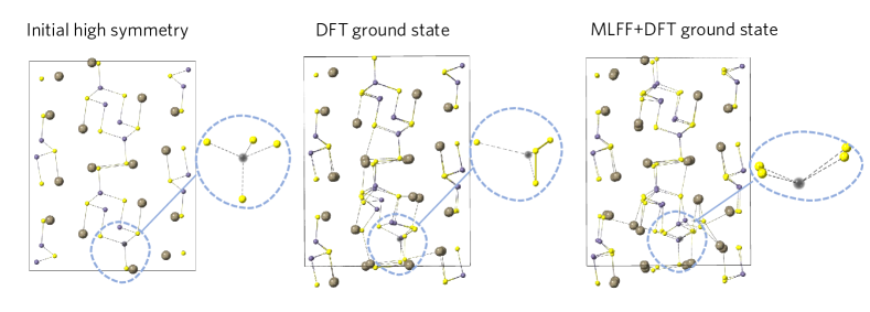
Figure S14: V${}_{\text{Ge,9}}$ in TlGeS2. Ground state structures identified with the DFT search (S trimer) and with the MLFF+DFT approach (one S dimer), with the second being $0.5\text{\,}\mathrm{e}\mathrm{V}$ lower in energy. The structure with only one S-S bond seems to be more favourable due to avoiding strain caused by the rearrangement of the atoms. For clarity, the initial high symmetry defect structure is shown on the left.

S3.3 Failed systems

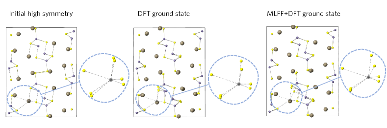
Figure S15: High symmetry (initial) and ground state structures of V${}_{\text{Tl,0}}$ in TlGeS2 identified with the DFT-only search and the MLFF+DFT approach. While the configuration identified with the DFT search is $0.1\text{\,}\mathrm{e}\mathrm{V}$ lower in energy than the MLFF+DFT structure, we note that the reconstruction motifs are very similar.

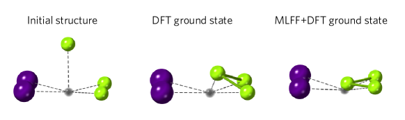
Figure S16: High symmetry (initial) and ground state structures of V${}_{\text{Bi}}$ in BiSeI identified with the DFT-only search and the MLFF+DFT approach. While the configuration identified with the DFT search is $0.2\text{\,}\mathrm{e}\mathrm{V}$ lower in energy than the MLFF+DFT structure, we note that the reconstruction motifs are similar, involving a Se trimer in both cases.

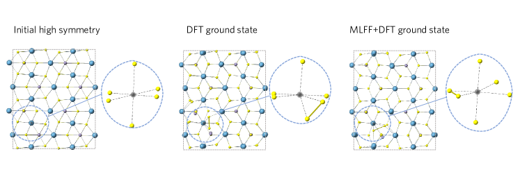
Figure S17: High symmetry (initial) and ground state structures of V${}_{\text{Ca,0}}$ in Ca2SnS4 identified with the DFT-only search and the MLFF+DFT approach. While the configuration identified with the DFT search is $0.7\text{\,}\mathrm{e}\mathrm{V}$ lower in energy than the MLFF+DFT structure, we note that the reconstruction motifs are similar, involving a S dimer in both cases.

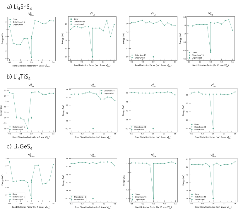
Figure S18: Energy vs distortion plots for all the cation vacancies in the test system Li4SnS4 (a) and the training compositions Li4TiS4 and Li4GeS4 (b, c). Note that most of the relaxations are trapped in high-energy minima, thus hindering learning the low-energy region of the PES for these systems. This trapping into high-energy basins can be avoided by reducing the magnitude of the rattle distortion that is applied with ShakeNBreak to the sampling structures.

S3.4 Acceleration factors

Table S12: Comparison of computing times for structure searching when using the full DFT approach and the MLFF+DFT approach. We compare the time required to run the structure searching relaxations when only using DFT (i.e. starting from the ShakeNBreak initial structures) and when pre-relaxing the structures with the MLFF. These timings are listed in the columns ‘DFT time’ (full DFT relaxation of ShakeNBreak structures), ‘MLFF time’ (DFT relaxation of the MLFF-relaxed ShakeNBreak structures) and ‘Inference time’ (MLFF relaxation of ShakeNBreak structures).

Host	Defect	Num atoms	Num electrons	DFT time (CPU h)	MLFF time (CPU h)	Inference time (GPU h)	Speedup
BiSeBr	V${}_{\rm Bi_{0}}$	71	657	4736.7	3742.7	0.05	1.3
BiSeI	V${}_{\rm Bi_{0}}$	71	657	5778.6	3160.8	0.04	1.8
Li4SnS4	V${}_{\rm Sn_{1}6}$	143	786	13976.7	18042.3	0.21	0.8
Li4SnS4	V${}_{\rm Li_{0}}$	143	797	11549.0	2576.1	0.18	4.5
Li4SnS4	V${}_{\rm Li_{4}}$	143	797	433083.1	6847.8	0.24	63.2
Li4SnS4	V${}_{\rm Li_{8}}$	143	797	41380.0	6205.6	0.15	6.7
CuSe	V${}_{\rm Cu_{0}}$	107	907	21196.8	969.0	0.06	21.9
CuSe	V${}_{\rm Cu_{4}}$	107	907	27734.9	1647.9	0.05	16.8
CuS	V${}_{\rm Cu_{0}}$	143	1213	30292.0	7821.3	0.03	3.9
CuS	V${}_{\rm Cu_{3}}$	143	1213	39892.4	3701.4	0.03	10.8

S4 Surrogate model for closely-related systems

To investigate whether targeting more similar systems would reduce the dataset size required for similar model performance, we developed a model for chalcohalide systems. We selected the chalcohalides from our dataset, resulting in 11 compositions (BiSCl, BiSBr, BiSI, BiSeCl, BiSeBr, BiSeI, SbSBr, SbSI, SbSeBr, SbSeI AgBiSCl2) (S19). Three of these (27%; BiSeCl, BiSeBr, BiSeI) were held out as the test set, and the remaining data was split into training and validation sets with 0.9 and 0.1 fractions , resulting in a training and validation sizes of 1476 and 164 configurations, respectively. The resulting training set was then increased by adding ten evenly spaced frames from the relaxation of each pristine host structure (110 configurations) — as this was observed to improve performance (S13, S20, S21).

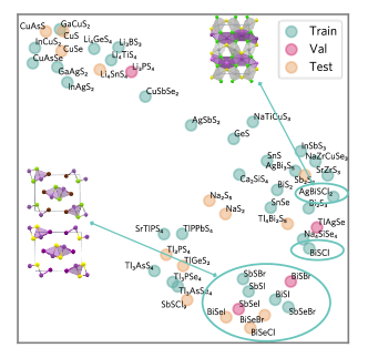
Figure S19: Plot of the first two principal components of the feature space for the pristine structures, showing the selection of the chalcohalide systems. The structures were encoded with the SOAP descriptor, whose dimensions were reduced for plotting with Principal Component Analysis.[91].

Table S13: Mean absolute errors, root mean squared errors and Spearman coefficients on the test set for the chalcohalide model when only training on defect data and when training on both defect and bulk data. The distribution of the absolute errors is shown in S20, S21.

Dataset	$\rm MAE_{E}$ (meV/atom)	$\rm RMSE_{E}$ (meV/atom)	$\rho$	$\rm MAE_{F}$ (meV/Å)	$\rm RMSE_{F}$ (meV/Å)	$\rm MAE_{S}$ (GPa)	$\rm RMSE_{S}$ (GPa)
Bulk + Defect	21.9	30.6	0.82	63.8	153.7	0.10	0.17
Defect only	21.3	23.1	0.72	97.6	175.2	0.10	0.16

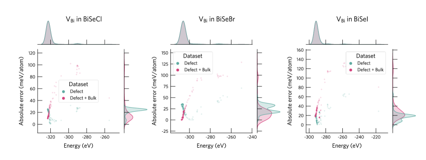
Figure S20: Comparison of absolute energy error distributions for the test systems when training on defect (green) and both defect and bulk data (pink). As seen for BiSeCl and BiSeBr, adding bulk data to the training set reduces the errors for the low-energy configurations.

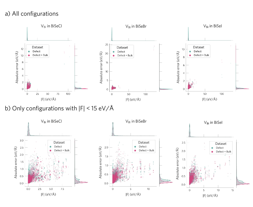
Figure S21: Comparison of absolute force error distributions for the test systems when training on defect (green) and both defect and bulk data (pink). a) All configurations and b) removing outliers with high forces ($|F|<15~{}\mathrm{eV}/\mathrm{\mathrm{\text{Å}}}$). Adding bulk data to the training set reduces the force errors for the low-energy configurations.

As shown in S14, the mean absolute errors are slightly lower than for the full model (trained on all compositions), confirming that smaller datasets can be used when targeting more similar host structures since their PES is easier to learn. After applying our MLFF+DFT approach to the test systems, it identifies the correct ground state for all three defects, while reducing the number of DFT calculations by 53%. Further, we note that the candidate structures selected in our approach (by relaxing the initial sampling structures with the MLFF and then selecting the structures with a unique SOAP fingerprint[91] for the defect site) target the low-energy region of the PES, as demonstrated in S22. Further, it also identifies two low-energy metastable structures that are missed with the DFT-only approach, validating that the model learns to suggest good candidate structures.

Table S14: Mean absolute errors and Spearman coefficients ($\rho$) for training, validation and test sets of the chalcohalide model (training on both defect and bulk data).

Set	$\rm E$ (meV/atom)	$\rm F$ (meV/Å)	$\rm S$ (GPa)	$\rho$
Train	19.2	51.0	0.06	0.92
Val	13.3	51.7	0.05	0.91
Test	21.9	63.7	0.10	0.82

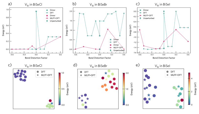
Figure S22: Comparison of DFT and MLFF+DFT approaches. (a, b, c) Plots of final (DFT) energy versus initial distortion for V${}_{\text{Bi}}$⁰ in BiSeCl, BiSeBr and BiSeI. The full DFT approach (green) is compared with our MLFF+DFT strategy (pink). Note that the MLFF+DFT successfully targets the low-energy regions of the PES. Further, we note that several low-energy metastable configurations are missed with the DFT-only approach but identified with the MLFF+DFT one. The label “Unperturbed” denotes the configuration obtained by relaxing the high symmetry ideal structure while the label “Dimer” denotes a targeted distortion that pushes two of the defect nearest neighbours towards each other. (c, d, e) 2D projection of structural similarity for final structures obtained with the full DFT (circles) and MLFF+DFT approach (stars), illustrating that the latter targets the low-energy regions of the PES (e.g. no red stars).

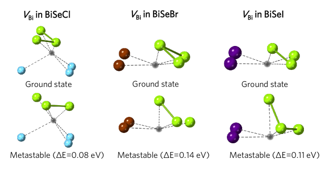
Figure S23: Ground state structures for V${}_{\text{Bi}}$ in BiSeCl, BiSeBr and BiSeI. On the bottom, the low-energy metastable configurations that are only identified with the MLFF+DFT strategy are shown.

S5 Extension to Alloys

Figure S24: Evolution of training and validation errors with epoch number. The validation errors obtained for the epoch with the lowest validation loss are shown at the top right of each subplot.

Table S15: Performance of the MLFF model on the CdSe_xTe_(1-x) systems. For each inequivalent defect in each alloy, we show the number of local minima identified by the DFT-based (coarser) search and by the MLFF finer search. When a more favourable ground state (GS) configuration is identified by the MLFF search, the energy lowering and the reconstruction driving it are shown.

x	Defects	Num. local minima in DFT PES	Num. local minima in MLFF PES	Novel GS? (eV)	Reconstruction
0.2	V${}_{\rm Cd_{0}}$	2	5	-0.3	Se-Te $\rightarrow$ Te-Te
0.2	V${}_{\rm Cd_{10}}$	2	6	-0.5	Se-Se $\rightarrow$ Se-Te
0.2	V${}_{\rm Cd_{1}}$	2	4	-0.6	Se-Se $\rightarrow$ Te-Te
0.2	V${}_{\rm Cd_{4}}$	2	4	0.0	Te-Te $\rightarrow$ Te-Te
0.3	V${}_{\rm Cd_{0}}$	2	5	-0.4	Se-Te $\rightarrow$ Te-Te
0.3	V${}_{\rm Cd_{21}}$	3	5	-0.2	Se-Se $\rightarrow$ Se-Te
0.3	V${}_{\rm Cd_{2}}$	2	6	0.0	Se-Se $\rightarrow$ Se-Se
0.3	V${}_{\rm Cd_{4}}$	2	4	-0.2	Se-Se $\rightarrow$ Se-Te
0.3	V${}_{\rm Cd_{5}}$	2	4	0.0	Te-Te $\rightarrow$ Te-Te
0.5	V${}_{\rm Cd_{0}}$	1	6	-0.7	Td$\rightarrow$ Te-Te
0.5	V${}_{\rm Cd_{4}}$	1	5	-0.5	Td $\rightarrow$ Te-Te
0.5	V${}_{\rm Cd_{1}}$	2	3	-0.5	Se-Te $\rightarrow$ Te-Te
0.5	V${}_{\rm Cd_{3}}$	2	4	-0.3	Se-Se $\rightarrow$ Se-Te
0.5	V${}_{\rm Cd_{5}}$	2	4	-0.4	Se-Se $\rightarrow$ Se-Se
0.6	V${}_{\rm Cd_{0}}$	2	4	-0.5	Se-Se $\rightarrow$ Se-Te
0.6	V${}_{\rm Cd_{2}}$	3	10	-0.1	Se-Se $\rightarrow$ Se-Te
0.6	V${}_{\rm Cd_{3}}$	2	5	0.0	Te-Te $\rightarrow$ Te-Te
0.6	V${}_{\rm Cd_{4}}$	3	3	0.0	Se-Se $\rightarrow$ Se-Se
0.8	V${}_{\rm Cd_{0}}$	3	5	-0.6	Se-Se $\rightarrow$ Se-Te
0.8	V${}_{\rm Cd_{1}}$	3	7	0.0	Se-Se $\rightarrow$ Se-Se
0.8	V${}_{\rm Cd_{25}}$	1	3	-0.6	Td $\rightarrow$ Te-Te
0.8	V${}_{\rm Cd_{3}}$	3	4	-0.3	Se-Te $\rightarrow$ Te-Te
0.9	V${}_{\rm Cd_{0}}$	1	4	-0.7	Td $\rightarrow$ Se-Te
0.9	V${}_{\rm Cd_{0}}$	3	6	0.0	Se-Se $\rightarrow$ Se-Se

References

- Sambur and Brgoch [2023] J. Sambur and J. Brgoch, Chem. Mater., 2023, 35, 7351–7354.
- Shockley and Read [1952] W. Shockley and W. T. Read, Phys. Rev., 1952, 87, 835–842.
- Kim et al. [2020] S. Kim, J. A. Márquez, T. Unold and A. Walsh, Energy Environ. Sci., 2020, 13, 1481–1491.
- Maier [2013] J. Maier, Angew. Chem. Int. Ed., 2013, 52, 4998–5026.
- Squires et al. [2022] A. G. Squires, D. W. Davies, S. Kim, D. O. Scanlon, A. Walsh and B. J. Morgan, Phys. Rev. Mater., 2022, 6, 085401.
- Li et al. [2020] W. Li, D. Wang, Y. Zhang, L. Tao, T. Wang, Y. Zou, Y. Wang, R. Chen and S. Wang, Adv. Mater., 2020, 32, 1907879.
- Pastor et al. [2022] E. Pastor, M. Sachs, S. Selim, J. R. Durrant, A. A. Bakulin and A. Walsh, Nat. Rev. Mater., 2022, 7, 503–521.
- Kehoe et al. [2011] A. B. Kehoe, D. O. Scanlon and G. W. Watson, Chem. Mater., 2011, 23, 4464–4468.
- Ivády et al. [2018] V. Ivády, I. A. Abrikosov and A. Gali, npj Comput Mater, 2018, 4, 76.
- Weber et al. [2010] J. R. Weber, W. F. Koehl, J. B. Varley, A. Janotti, B. B. Buckley, C. G. V. de Walle and D. D. Awschalom, Proc. Natl. Acad. Sci. U.S.A., 2010, 107, 8513–8518.
- Thomas et al. [2023] J. Thomas, W. Chen, Y. Xiong, B. Barker, J. Zhou, W. Chen, A. Rossi, N. Kelly, Z. Yu, D. Zhou, S. Kumari, E. Barnard, J. Robinson, M. Terrones, A. Schwartzberg, D. F. Ogletree, E. Rotenberg, M. Noack, S. Griffin, A. Raja, D. Strubbe, G.-M. Rignanese, A. Weber-Bargioni and G. Hautier, 2023, arXiv:cond-mat/2309.08032.
- Dreyer et al. [2018] C. E. Dreyer, A. Alkauskas, J. L. Lyons, A. Janotti and C. G. Van de Walle, Annu. Rev. Mater. Res., 2018, 48, 1–26.
- Yan et al. [2024] Q. Yan, S. Kar, S. Chowdhury and A. Bansil, Adv Mater, 2024, 2303098.
- Davidsson et al. [2023] J. Davidsson, F. Bertoldo, K. S. Thygesen and R. Armiento, npj 2D Mater. Appl., 2023, 7, 26.
- Sluydts et al. [2016] M. Sluydts, M. Pieters, J. Vanhellemont, V. V. Speybroeck and S. Cottenier, Chem. Mater., 2016, 29, 975–984.
- Bertoldo et al. [2022] F. Bertoldo, S. Ali, S. Manti and K. S. Thygesen, npj Comput Mater, 2022, 8, 56.
- Huang et al. [2023] P. Huang, R. Lukin, M. Faleev, N. Kazeev, A. R. Al-Maeeni, D. V. Andreeva, A. Ustyuzhanin, A. Tormasov, A. H. Castro Neto and K. S. Novoselov, npj 2D Mater Appl, 2023, 7, 1–10.
- Medasani et al. [2016] B. Medasani, A. Gamst, H. Ding, W. Chen, K. A. Persson, M. Asta, A. Canning and M. Haranczyk, npj Comput Mater, 2016, 2, 1–10.
- Rahman et al. [2023] M. H. Rahman, P. Gollapalli, P. Manganaris, S. K. Yadav, G. Pilania, B. DeCost, K. Choudhary and A. Mannodi-Kanakkithodi, 2023, arXiv:cond-mat/2309.06423.
- Ivanov et al. [2023] V. Ivanov, A. Ivanov, J. Simoni, P. Parajuli, B. Kanté, T. Schenkel and L. Tan, 2023, arXiv:quant-ph/2303.16283.
- Kumagai et al. [2021] Y. Kumagai, N. Tsunoda, A. Takahashi and F. Oba, Phys. Rev. Mater., 2021, 5, 123803.
- Deml et al. [2015] A. M. Deml, A. M. Holder, R. P. O’Hayre, C. B. Musgrave and V. Stevanović, J. Phys. Chem. Lett., 2015, 6, 1948–1953.
- Broberg et al. [2023] D. Broberg, K. Bystrom, S. Srivastava, D. Dahliah, B. A. D. Williamson, L. Weston, D. O. Scanlon, G.-M. Rignanese, S. Dwaraknath, J. Varley, K. A. Persson, M. Asta and G. Hautier, npj Comput Mater, 2023, 9, 72.
- Mannodi-Kanakkithodi et al. [2022] A. Mannodi-Kanakkithodi, X. Xiang, L. Jacoby, R. Biegaj, S. T. Dunham, D. R. Gamelin and M. K. Chan, Patterns, 2022, 3, 100450.
- Varley et al. [2017] J. B. Varley, A. Samanta and V. Lordi, J. Phys. Chem. Lett., 2017, 8, 5059–5063.
- Wan et al. [2021] Z. Wan, Q.-D. Wang, D. Liu and J. Liang, Phys. Chem. Chem. Phys., 2021, 23, 15675–15684.
- Wexler et al. [2021] R. B. Wexler, G. S. Gautam, E. B. Stechel and E. A. Carter, J. Am. Chem. Soc., 2021, 143, 13212–13227.
- Frey et al. [2020] N. C. Frey, D. Akinwande, D. Jariwala and V. B. Shenoy, ACS Nano, 2020, 14, 13406–13417.
- Sharma et al. [2020] V. Sharma, P. Kumar, P. Dev and G. Pilania, J. Appl. Phys., 2020, 128, 034902.
- Baldassarri et al. [2023] B. Baldassarri, J. He, A. Gopakumar, S. Griesemer, A. J. A. Salgado-Casanova, T.-C. Liu, S. B. Torrisi and C. Wolverton, Chem. Mater., 2023, 35, 10619–10634.
- Park et al. [0] S. Park, N. Lee, J. O. Park, J. Park, Y. S. Heo and J. Lee, ACS Mater. Lett., 0, 0, 66–72.
- Kazeev et al. [2023] N. Kazeev, A. R. Al-Maeeni, I. Romanov, M. Faleev, R. Lukin, A. Tormasov, A. H. Castro Neto, K. S. Novoselov, P. Huang and A. Ustyuzhanin, npj Comput Mater, 2023, 9, 113.
- Choudhary and Sumpter [2023] K. Choudhary and B. G. Sumpter, AIP Adv., 2023, 13, 095109.
- Zhao et al. [2023] X. Zhao, S. Yu, J. Zheng, M. J. Reece and R.-Z. Zhang, J. Eur. Ceram. Soc., 2023, 43, 1315–1321.
- Manzoor et al. [2021] A. Manzoor, G. Arora, B. Jerome, N. Linton, B. Norman and D. S. Aidhy, Front. Mater., 2021, 8, 673574.
- Polak et al. [2022] M. P. Polak, R. Jacobs, A. Mannodi-Kanakkithodi, M. K. Y. Chan and D. Morgan, J. Chem. Phys., 2022, 156, 114110.
- Witman et al. [2023] M. D. Witman, A. Goyal, T. Ogitsu, A. H. McDaniel and S. Lany, Nat Comput Sci, 2023, 3, 675–686.
- Arrigoni and Madsen [2021] M. Arrigoni and G. K. H. Madsen, npj Comput. Mater., 2021, 7, 1–13.
- Kavanagh et al. [2021] S. R. Kavanagh, A. Walsh and D. O. Scanlon, ACS Energy Lett., 2021, 6, 1392–1398.
- Mosquera-Lois and Kavanagh [2021] I. Mosquera-Lois and S. R. Kavanagh, Matter, 2021, 4, 2602–2605.
- Mosquera-Lois et al. [2023] I. Mosquera-Lois, S. R. Kavanagh, A. Walsh and D. O. Scanlon, npj Comput. Mater., 2023, 9, 1–11.
- Wang et al. [2023] X. Wang, S. R. Kavanagh, D. O. Scanlon and A. Walsh, Phys. Rev. B, 2023, 108, 134102.
- Morris et al. [2009] A. J. Morris, C. J. Pickard and R. J. Needs, Phys. Rev. B, 2009, 80, 144112.
- Mulroue et al. [2011] J. Mulroue, A. J. Morris and D. M. Duffy, Phys. Rev. B, 2011, 84, 094118.
- Al-Mushadani and Needs [2003] O. K. Al-Mushadani and R. J. Needs, Phys. Rev. B, 2003, 68, 235205.
- Kononov et al. [2023] A. Kononov, C.-W. Lee, E. Shapera and A. Schleife, J. Phys. Condens., 2023, 35, 334002.
- Schaarschmidt et al. [2022] M. Schaarschmidt, M. Riviere, A. M. Ganose, J. S. Spencer, A. L. Gaunt, J. Kirkpatrick, S. Axelrod, P. W. Battaglia and J. Godwin, 2022, arXiv:cond-mat/2209.12466.
- Lan et al. [2023] J. Lan, A. Palizhati, M. Shuaibi, B. M. Wood, B. Wander, A. Das, M. Uyttendaele, C. L. Zitnick and Z. W. Ulissi, npj Comput Mater, 2023, 9, 172.
- Lany and Zunger [2004] S. Lany and A. Zunger, Phys. Rev. Lett., 2004, 93, 156404.
- Kang and Wang [2017] J. Kang and L.-W. Wang, J. Phys. Chem. Lett., 2017, 8, 489–493.
- Wilson et al. [2008] D. J. Wilson, A. A. Sokol, S. A. French and C. R. A. Catlow, Phys. Rev. B, 2008, 77, 064115.
- Zhao et al. [2016] Y. Zhao, W. Zhou, W. Ma, S. Meng, H. Li, J. Wei, R. Fu, K. Liu, D. Yu and Q. Zhao, ACS Energy Lett., 2016, 1, 266–272.
- Ágoston et al. [2009] P. Ágoston, P. Erhart, A. Klein and K. Albe, J. Phys. Condens. Matter, 2009, 21, 455801.
- Han et al. [2017] D. Han, M.-H. Du, C.-M. Dai, D. Sun and S. Chen, J. Mater. Chem. A, 2017, 5, 6200–6210.
- Meggiolaro et al. [2020] D. Meggiolaro, D. Ricciarelli, A. A. Alasmari, F. A. S. Alasmary and F. De Angelis, J. Phys. Chem. Lett., 2020, 11, 3546–3556.
- Erhart et al. [2005] P. Erhart, A. Klein and K. Albe, Phys. Rev. B, 2005, 72, 085213.
- Sokol et al. [2010] A. A. Sokol, A. Walsh and C. R. A. Catlow, Chem. Phys. Lett., 2010, 492, 44–48.
- Evarestov et al. [1996] R. A. Evarestov, P. W. M. Jacobs and A. V. Leko, Phys. Rev. B, 1996, 54, 8969–8972.
- Kotomin and Popov [1998] E. A. Kotomin and A. I. Popov, Nucl. Instrum. Methods Phys. Res. B, 1998, 141, 1–15.
- Burbano et al. [2011] M. Burbano, D. O. Scanlon and G. W. Watson, J. Am. Chem. Soc., 2011, 133, 15065–15072.
- Scanlon and Watson [2012] D. O. Scanlon and G. W. Watson, J. Mater. Chem., 2012, 22, 25236–25245.
- Godinho et al. [2009] K. G. Godinho, A. Walsh and G. W. Watson, J. Phys. Chem. C, 2009, 113, 439–448.
- Scanlon et al. [2011] D. O. Scanlon, A. B. Kehoe, G. W. Watson, M. O. Jones, W. I. F. David, D. J. Payne, R. G. Egdell, P. P. Edwards and A. Walsh, Phys. Rev. Lett., 2011, 107, 246402.
- Keating et al. [2012] P. R. L. Keating, D. O. Scanlon, B. J. Morgan, N. M. Galea and G. W. Watson, J. Phys. Chem. C, 2012, 116, 2443–2452.
- Walsh et al. [2009] A. Walsh, J. L. F. Da Silva and S.-H. Wei, Chem. Mater., 2009, 21, 5119–5124.
- Whalley et al. [2017] L. D. Whalley, R. Crespo-Otero and A. Walsh, ACS Energy Lett., 2017, 2, 2713–2714.
- Agiorgousis et al. [2014] M. L. Agiorgousis, Y.-Y. Sun, H. Zeng and S. Zhang, J. Am. Chem. Soc., 2014, 136, 14570–14575.
- Whalley et al. [2021] L. D. Whalley, P. van Gerwen, J. M. Frost, S. Kim, S. N. Hood and A. Walsh, J. Am. Chem. Soc., 2021, 143, 9123–9128.
- Motti et al. [2019] S. G. Motti, D. Meggiolaro, S. Martani, R. Sorrentino, A. J. Barker, F. De Angelis and A. Petrozza, Adv Mater, 2019, 31, 1901183.
- Xiao et al. [2016] Z. Xiao, W. Meng, J. Wang and Y. Yan, Phys. Chem. Chem. Phys., 2016, 18, 25786–25790.
- Na-Phattalung et al. [2006] S. Na-Phattalung, M. F. Smith, K. Kim, M.-H. Du, S.-H. Wei, S. B. Zhang and S. Limpijumnong, Phys. Rev. B, 2006, 73, 125205.
- Li et al. [2023] K. Li, J. Willis, S. R. Kavanagh and D. O. Scanlon, 2023, chemrxiv-2023-8l7pb.
- Scanlon [2013] D. O. Scanlon, Phys. Rev. B, 2013, 87, 161201.
- Cen et al. [2023] J. Cen, B. Zhu, S. R. Kavanagh, A. G. Squires and D. O. Scanlon, J. Mater. Chem. A, 2023, 11, 13353–13370.
- Mosquera-Lois et al. [2022] I. Mosquera-Lois, S. R. Kavanagh, A. Walsh and D. O. Scanlon, J. Open Source Softw., 2022, 7, 4817.
- Chen and Ong [2022] C. Chen and S. P. Ong, Nat Comput Sci, 2022, 2, 718–728.
- Qi et al. [2023] J. Qi, T. W. Ko, B. C. Wood, T. A. Pham and S. P. Ong, 2023, arXiv:cond-mat/22307.13710.
- van der Maaten and Hinton [2008] L. van der Maaten and G. Hinton, J. Mach. Learn. Res., 2008, 9, 2579–2605.
- Hinton and Roweis [2002] G. E. Hinton and S. Roweis, Adv Neural Inf Process Syst, 2002, 15, 857–864.
- Chen et al. [2019] C. Chen, W. Ye, Y. Zuo, C. Zheng and S. P. Ong, Chem Mater, 2019, 31, 3564–3572.
- [81] NIST Chemistry WebBook, https://doi.org/10.18434/M32147, (accessed May 2023).
- Deng et al. [2023] B. Deng, P. Zhong, K. Jun, J. Riebesell, K. Han, C. J. Bartel and G. Ceder, Nat. Mach. Intell., 2023, 5, 1031–1041.
- Merchant et al. [2023] A. Merchant, S. Batzner, S. S. Schoenholz, M. Aykol, G. Cheon and E. D. Cubuk, Nature, 2023, 624, 80–85.
- Batatia et al. [2024] I. Batatia, P. Benner, Y. Chiang, A. M. Elena, D. P. Kovács, J. Riebesell, X. R. Advincula, M. Asta, W. J. Baldwin, N. Bernstein, A. Bhowmik, S. M. Blau, V. Cărare, J. P. Darby, S. De, F. Della Pia, V. L. Deringer, R. Elijošius, Z. El-Machachi, E. Fako, A. C. Ferrari, A. Genreith-Schriever, J. George, R. E. A. Goodall, C. P. Grey, S. Han, W. Handley, H. H. Heenen, K. Hermansson, C. Holm, J. Jaafar, S. Hofmann, K. S. Jakob, H. Jung, V. Kapil, A. D. Kaplan, N. Karimitari, N. Kroupa, J. Kullgren, M. C. Kuner, D. Kuryla, G. Liepuoniute, J. T. Margraf, I.-B. Magdău, A. Michaelides, J. H. Moore, A. A. Naik, S. P. Niblett, S. W. Norwood, N. O’Neill, C. Ortner, K. A. Persson, K. Reuter, A. S. Rosen, L. L. Schaaf, C. Schran, E. Sivonxay, T. K. Stenczel, V. Svahn, C. Sutton, C. van der Oord, E. Varga-Umbrich, T. Vegge, M. Vondrák, Y. Wang, W. C. Witt, F. Zills and G. Csányi, 2024, arXiv:physics.chem-ph/2401.00096.
- Batatia et al. [2022] I. Batatia, D. P. Kovács, G. N. C. Simm, C. Ortner and G. Csányi, 2022, arXiv:stat.ML/2206.07697.
- [86] C. Chen and S. P. Ong, M3GNet (version 0.2.4), 2023.
- Salzbrenner et al. [2023] P. T. Salzbrenner, S. H. Joo, L. J. Conway, P. I. C. Cooke, B. Zhu, M. P. Matraszek, W. C. Witt and C. J. Pickard, J. Chem. Phys., 2023, 159, 144801.
- Pickard [2022] C. J. Pickard, Phys. Rev. B, 2022, 106, 014102.
- Musielewicz et al. [2022] J. Musielewicz, X. Wang, T. Tian and Z. Ulissi, Mach. Learn. Technol., 2022, 3, 03LT01.
- Jung et al. [2023] H. Jung, L. Sauerland, S. Stocker, K. Reuter and J. T. Margraf, npj Comput Mater, 2023, 9, 114.
- Bartók et al. [2013] A. P. Bartók, R. Kondor and G. Csányi, Phys. Rev. B, 2013, 87, 184115.
- Hu [2023] Y.-J. Hu, Comput. Mater. Sci., 2023, 216, 111831.
- Piochaud et al. [2014] J. B. Piochaud, T. P. C. Klaver, G. Adjanor, P. Olsson, C. Domain and C. S. Becquart, Phys. Rev. B, 2014, 89, 024101.
- Guan et al. [2020] H. Guan, S. Huang, J. Ding, F. Tian, Q. Xu and J. Zhao, Acta Mater., 2020, 187, 122–134.
- Rio et al. [2011] E. d. Rio, J. M. Sampedro, H. Dogo, M. J. Caturla, M. Caro, A. Caro and J. M. Perlado, J. Nucl. Mater., 2011, 408, 18–24.
- Zhang et al. [2015] Y. Zhang, G. M. Stocks, K. Jin, C. Lu, H. Bei, B. C. Sales, L. Wang, L. K. Béland, R. E. Stoller, G. D. Samolyuk, M. Caro, A. Caro and W. J. Weber, Nat Commun, 2015, 6, 8736.
- Zhang et al. [2017] Y. Zhang, S. Zhao, W. J. Weber, K. Nordlund, F. Granberg and F. Djurabekova, Curr. Opin. Solid State Mater. Sci., 2017, 21, 221–237.
- Arora et al. [2021] G. Arora, G. Bonny, N. Castin and D. S. Aidhy, Acta Mater, 2021, 15, 100974.
- Zhao et al. [2016] S. Zhao, G. M. Stocks and Y. Zhang, Phys. Chem. Chem. Phys., 2016, 18, 24043–24056.
- Manzoor and Zhang [2022] A. Manzoor and Y. Zhang, JOM, 2022, 74, 4107–4120.
- Zhao et al. [2018] S. Zhao, T. Egami, G. M. Stocks and Y. Zhang, Phys. Rev. Mater., 2018, 2, 013602.
- Li et al. [2019] C. Li, J. Yin, K. Odbadrakh, B. C. Sales, S. J. Zinkle, G. M. Stocks and B. D. Wirth, J. Appl. Phys, 2019, 125, 155103.
- Manzoor et al. [2021] A. Manzoor, Y. Zhang and D. S. Aidhy, Comput. Mater. Sci., 2021, 198, 110669.
- Muzyk et al. [2011] M. Muzyk, D. Nguyen-Manh, K. J. Kurzydłowski, N. L. Baluc and S. L. Dudarev, Phys. Rev. B, 2011, 84, 104115.
- Wang et al. [2022] Y. Wang, S. R. Kavanagh, I. Burgués-Ceballos, A. Walsh, D. O. Scanlon and G. Konstantatos, Nat. Photon., 2022, 16, 235–241.
- Williford et al. [1999] R. Williford, W. Weber, R. Devanathan and J. Gale, J. Electroceramics, 1999, 3, 409–424.
- Quadir et al. [2022] S. Quadir, M. Qorbani, A. Sabbah, T.-S. Wu, A. k. Anbalagan, W.-T. Chen, S. Meledath Valiyaveettil, H.-T. Thong, C.-W. Wang, C.-Y. Chen, C.-H. Lee, K.-H. Chen and L.-C. Chen, Chem. Mater., 2022, 34, 7058–7068.
- Morrow et al. [2023] J. D. Morrow, C. Ugwumadu, D. A. Drabold, S. R. Elliott, A. L. Goodwin and V. L. Deringer, 2023, arXiv:cond-mat/2308.16868.
- Riebesell et al. [2023] J. Riebesell, R. E. A. Goodall, A. Jain, P. Benner, K. A. Persson and A. A. Lee, 2023, arXiv:cond-mat/2308.14920.
- Shimizu et al. [2022] K. Shimizu, Y. Dou, E. F. Arguelles, T. Moriya, E. Minamitani and S. Watanabe, Phys. Rev. B, 2022, 106, 054108.
- Ko et al. [2021] T. W. Ko, J. A. Finkler, S. Goedecker and J. Behler, Acc. Chem. Res., 2021, 54, 808–817.
- Kavanagh et al. [2022] S. R. Kavanagh, D. O. Scanlon, A. Walsh and C. Freysoldt, Faraday Discuss., 2022, 239, 339–356.
- Mosquera-Lois et al. [2023] I. Mosquera-Lois, S. R. Kavanagh, J. Klarbring, K. Tolborg and A. Walsh, Chem. Soc. Rev., 2023, 52, 5812–5826.
- Pols et al. [2023] M. Pols, V. Brouwers, S. Calero and S. Tao, Chem. Commun., 2023, 59, 4660–4663.
- Freysoldt et al. [2014] C. Freysoldt, B. Grabowski, T. Hickel, J. Neugebauer, G. Kresse, A. Janotti and C. G. Van de Walle, Rev. Mod. Phys., 2014, 86, 253–305.
- Lany and Zunger [2008] S. Lany and A. Zunger, Phys. Rev. B, 2008, 78, 235104.
- Heyd et al. [2003] J. Heyd, G. E. Scuseria and M. Ernzerhof, J. Chem. Phys., 2003, 118, 8207–8215.
- Kresse and Furthmüller [1996] G. Kresse and J. Furthmüller, Comput. Mater. Sci., 1996, 6, 15–50.
- Kresse and Hafner [1993] G. Kresse and J. Hafner, Phys. Rev. B, 1993, 47, 558–561.
- Kresse and Hafner [1994] G. Kresse and J. Hafner, Phys. Rev. B, 1994, 49, 14251–14269.
- Pizzi et al. [2016] G. Pizzi, A. Cepellotti, R. Sabatini, N. Marzari and B. Kozinsky, Comput. Mater. Sci., 2016, 111, 218–230.
- Uhrin et al. [2021] M. Uhrin, S. P. Huber, J. Yu, N. Marzari and G. Pizzi, Comput. Mater. Sci., 2021, 187, 110086.
- Huber et al. [2020] S. P. Huber, S. Zoupanos, M. Uhrin, L. Talirz, L. Kahle, R. Häuselmann, D. Gresch, T. Müller, A. V. Yakutovich, C. W. Andersen, F. F. Ramirez, C. S. Adorf, F. Gargiulo, S. Kumbhar, E. Passaro, C. Johnston, A. Merkys, A. Cepellotti, N. Mounet, N. Marzari, B. Kozinsky and G. Pizzi, Sci. Data, 2020, 7, 300.
- Ong et al. [2013] S. P. Ong, W. D. Richards, A. Jain, G. Hautier, M. Kocher, S. Cholia, D. Gunter, V. L. Chevrier, K. A. Persson and G. Ceder, Comput. Mater. Sci., 2013, 68, 314–319.
- Jain et al. [2013] A. Jain, S. P. Ong, G. Hautier, W. Chen, W. D. Richards, S. Dacek, S. Cholia, D. Gunter, D. Skinner, G. Ceder and K. A. Persson, APL Materials, 2013, 1, 011002.
- Ong et al. [2015] S. P. Ong, S. Cholia, A. Jain, M. Brafman, D. Gunter, G. Ceder and K. A. Persson, Comput. Mater. Sci., 2015, 97, 209–215.
- [127] J.-X. Shen and J. B. Varley, pymatgen-analysis-defects (version 2023.10.19 ), 2023.
- Larsen et al. [2017] A. H. Larsen, J. J. Mortensen, J. Blomqvist, I. E. Castelli, R. Christensen, M. Dułak, J. Friis, M. N. Groves, B. Hammer, C. Hargus, E. D. Hermes, P. C. Jennings, P. B. Jensen, J. Kermode, J. R. Kitchin, E. L. Kolsbjerg, J. Kubal, K. Kaasbjerg, S. Lysgaard, J. B. Maronsson, T. Maxson, T. Olsen, L. Pastewka, A. Peterson, C. Rostgaard, J. Schiøtz, O. Schütt, M. Strange, K. S. Thygesen, T. Vegge, L. Vilhelmsen, M. Walter, Z. Zeng and K. W. Jacobsen, J. Condens. Matter Phys., 2017, 29, 273002.
- [129] S. R. Kavanagh, K. Brlec, B. Zhu, A. Nicolson, S. Hachmioune, S. Aggarwal, A. Walsh and D. O. Scanlon, Defect Oriented Python Environment Distribution (DOPED) (version 1.1.2), 2023.
- Bitzek et al. [2006] E. Bitzek, P. Koskinen, F. Gähler, M. Moseler and P. Gumbsch, Phys. Rev. Lett., 2006, 97, 170201.
- Morrow et al. [2023] J. D. Morrow, J. L. A. Gardner and V. L. Deringer, J. Chem. Phys., 2023, 158, 121501.