Biological species delimitation based on genetic and spatial dissimilarity: a comparative study

Abstract

The delimitation of biological species, i.e., deciding which individuals belong to the same species and whether and how many different species are represented in a data set, is key to the conservation of biodiversity. Much existing work uses only genetic data for species delimitation, often employing some kind of cluster analysis. This can be misleading, because geographically distant groups of individuals can be genetically quite different even if they belong to the same species. This paper investigates the problem of testing whether two potentially separated groups of individuals can belong to a single species or not based on genetic and spatial data. Various approaches are compared (some of which already exist in the literature) based on simulated metapopulations generated with SLiM and GSpace - two software packages that can simulate spatially-explicit genetic data at an individual level. Approaches involve partial Mantel testing, maximum likelihood mixed-effects models with a population effect, and jackknife-based homogeneity tests. A key challenge is that most tests perform on genetic and geographical distance data, violating standard independence assumptions. Simulations showed that partial Mantel tests and mixed-effects models have larger power than jackknife-based methods, but tend to display type-I-error rates slightly above the significance level. Moreover, a multiple regression model neglecting the dependence in the dissimilarities did not show inflated type-I-error rate. An application on brassy ringlets concludes the paper.

1 Introduction

The delimitation of biological species consists in using empirical data to determine which groups of individual organisms constitute different populations of a single species and which constitute different species [47]. Species delimitation is crucial to preserve biodiversity and has applications in several areas, such as ecology and medicine [9]. It is closely related to species conceptualization [14, 23], a long-standing problem that goes beyond the scope of this work. The empirical data employed to delimit species can be molecular (see, e.g., [47] for a review), morphological [20], behavioural [53], ecological [48, 49], etc., and integrative approaches using different types of data [15] and methods [10] are recommended.
Also spatial information is key for this task, as witnessed by the increase in publications in the field of landscape genetics [59], which combines population genetics and landscape ecology [3]. Neglecting geographic information when delimiting species can lead to the overestimation of the genetic structure in the data [18]. This is more likely to happen in the presence of spatial patterns of genetic differentiation, such as isolation by distance [[, IBD;]]ishida2009: clustering methods might wrongly assign individuals to different groups given that their genetic dissimilarity increases with geographic separation [8], violating the assumption of random mating within the population (panmixia).
A way to include spatial information in molecular species delimitation routines is to study the relationship between genetic dissimilarities and geographic distance. The investigation of this relationship has a long tradition in the population genetics literature, where it was pursued to study migration models [29] or estimate demographic parameters [56, 50, 13]. While isolation by distance assumes that the genetic dissimilarity between two individuals simply increases with the Euclidean distance (or, if we deal with latitude and longitude, the great-circle distance, i.e., the shortest distance between two locations on the surface of a sphere), isolation by resistance [[, IBR;]]mcrae2006 takes into account landscape features such as rivers and heights: this translates in developments like the least-cost path approach [1], the circuit-based framework [40] or the least-cost transect analysis [62], in which a more sophisticated landscape dissimilarity measure replaces the Euclidean distance in the attempt to explain genetic dissimilarities between individuals. In this perspective, IBR or isolation by environment [68] models are tested against the IBD model, which is seen as a null or baseline model [36].
This is where the study of the relationship between genetic and geographic dissimilarity and species delimitation come into contact. Consider a setup with two putative groups of individuals to be tested for conspecificity: for every pair of individuals in the sample, a grouping dissimilarity is computed, that takes value $1$ when they belong to different groups and $0$ otherwise. The impact of grouping on the genetic dissimilarity can be quantified controlling for the effect of geographic distance: if the genetic structure is positively associated with the grouping dissimilarity even after accounting for the Euclidean distance, this means that there is evidence that the two groups represent distinct species, since their molecular differences cannot be explained by geographic separation. This idea was applied by [41], who resorted to permutation-based partial Mantel tests [[, PMT;]]SLS86 to assess the significance of the partial correlation coefficient between genetic and grouping dissimilarities given the geographic distance. A hierarchical species delimitation testing protocol based on the relationship between genetic and geographic dissimilarities was developed for the same data problem by [25]. The maximum likelihood population effects model proposed by [13] can be extended and adapted to the same task. Also, partial Mantel tests in [41] can be carried out using jackknife or bootstrap instead of permutations. All these techniques take into account the dependence between dissimilarities involving the same individual. A multiple regression with genetic dissimilarities as response and geographic and grouping dissimilarities as explanatory variables neglects these data features and treats all dissimilarities as independent. A fixed-effects model similar to this was used by [58] to integrate a rich molecular species delimitation analysis.
There exists only anecdotal evidence of the performance of the methods in [41], [58] and [25] The study presented here consists in a systematic comparison of the type-I-error rate and power of the aforementioned methods based on spatially-explicit genetic simulations performed by GSpace [67] and SLiM [21] software. A jackknife or bootstrap-based PMT and an adaptation of the method in [13] to the purpose of species delimitation are also introduced and involved in the comparisons.
This paper is organized as follows: the data and distances are introduced in section 2, then all methods are discussed in section 3. The two simulators used in this study and the results obtained with them are discussed in section 4. An application on the data examined by [20] concludes the paper.

2 Data and dissimilarities

Spatially-explicit genetic data consists of individuals carrying information about their location and genetic make-up. Methods will be applied on individuals from two groups, with known membership. Hence, two columns will correspond to the unit’s coordinates (northings and eastings, latitude and longitude, etc.), one column will report the group labels (either group $1$ or $2$) and the other $P$ columns will be loci (locations on the DNA). Unless otherwise stated, individual-level codominant data, such as SNPs or microsatellites, with diploid genotypes [[]ch. 3]balkenhol2015 will be considered: this means that each locus will contain two alleles. These are represented in the literature by pairs of characters or strings: alleles like B [24] or 219 [51] will form diploid loci like BA and 219201. The resulting $n\times(P+3)$ data frame will be denoted by

$$\mathbf{Z}=\begin{pmatrix}\mathbf{z}_{1}\\ \vdots\\ \mathbf{z}_{n}\\ \end{pmatrix}=\begin{pmatrix}z_{1}^{x}&z_{1}^{y}&z_{1}^{c}&Z_{1}^{1}&\cdots&Z_{1}^{P}\\ z_{2}^{x}&z_{2}^{y}&z_{2}^{c}&Z_{2}^{1}&\cdots&Z_{2}^{P}\\ \vdots&\vdots&\vdots&\ddots&\vdots\\ z_{n}^{x}&z_{n}^{y}&z_{n}^{c}&Z_{n}^{1}&\cdots&Z_{n}^{P}\\ \end{pmatrix}\,,$$

where each observed locus $Z_{i}^{p}$, $p=1,\ldots,P$, is a set of characters, like $\{A,B\}$ for heterozygous loci (BA) or $\{B\}$ for homozygous ones (BB); also note that, in the sets, alleles are arranged in lexicographical order because their original ordering is not of interest in this study. Each $\mathbf{z}_{i}$ is a $1\times(P+3)$ vector representing the i^th individual.
In this study, the Euclidean distance will be employed as geographic distance (subscript $x$):

$$d_{x}(\mathbf{z}_{i},\mathbf{z}_{j})=\sqrt{(z_{i}^{x}-z_{j}^{x})^{2}+(z_{i}^{y}-z_{j}^{y})^{2}}\,.$$

As genetic dissimilarity (subscript $y$), the shared allele dissimilarity [7] will be used:

$$d_{y}(\mathbf{z}_{i},\mathbf{z}_{j})=1-\frac{1}{2P}\sum_{p=1}^{P}\left|Z_{i}^{p}\cap Z_{j}^{p}\right|\cdot\left[1+\mathbbm{1}\left(|Z_{i}^{p}|+|Z_{j}^{p}|=2\right)\right],$$ (2.1)

where $\mathbbm{1}(\text{condition})=1$ if the condition is true and zero otherwise. For instance, given the toy data frame

$$\mathbf{Z}=\begin{pmatrix}z_{1}^{x}&z_{1}^{y}&z_{1}^{c}&\{A\}&\{B\}&\{A,C\}\\ z_{2}^{x}&z_{2}^{y}&z_{2}^{c}&\{A,B\}&\{A,B\}&\{B,C\}\\ z_{3}^{x}&z_{3}^{y}&z_{3}^{c}&\{C\}&\{A\}&\{C\}\\ \end{pmatrix},$$

we get $d_{y}(\mathbf{z}_{1},\mathbf{z}_{2})=1/2$, $d_{y}(\mathbf{z}_{1},\mathbf{z}_{3})=5/6$ and $d_{y}(\mathbf{z}_{2},\mathbf{z}_{3})=2/3$. In this study, this dissimilarity was computed with the R package prabclus [24]. It is easy to see that, the larger $P$, the finer is the quantification of the genetic dissimilarity between two species, as more sites are available for the comparison of two individuals’ genetic information.
Assume to have $n_{1}=|\{i:z_{i}^{c}=1\}|$ individuals belonging to cluster 1 and $n_{2}=|\{i:z_{i}^{c}=2\}|$ individuals belonging to cluster 2: they represent the two candidate (or putative) species to be tested for conspecificity. In practice, this grouping information can be based on morphological, behavioural or even spatial grounds or can simply represent the researcher’s hypothesis. Given the cluster sizes $n_{1}$ and $n_{2}$, the number of geographic distances in the dataset will amount to:

$$\frac{1}{2}(n_{1}+n_{2})(n_{1}+n_{2}-1)=\underbrace{\frac{1}{2}n_{1}(n_{1}-1)}_{\text{within group 1}}+\underbrace{\frac{1}{2}n_{2}(n_{2}-1)}_{\text{within group 2}}+\underbrace{n_{1}n_{2}}_{\text{between groups}}\,,$$

to be stored in the following $n\times n$ block matrix, with $n=n_{1}+n_{2}$,

$$\mathbf{D}_{x} =\left(\begin{array}[]{c|c}\mathbf{D}_{x}^{11}&\mathbf{D}_{x}^{12}\\ \hline\cr\mathbf{D}_{x}^{21}&\mathbf{D}_{x}^{22}\\ \end{array}\right)$$

$$=\leavevmode\resizebox{390.25534pt}{}{ $\left(\begin{array}[]{cccc|ccc}0&d_{x}(\mathbf{z}_{1},\mathbf{z}_{2})&\cdots&d_{x}(\mathbf{z}_{1},\mathbf{z}_{n_{1}})&d_{x}(\mathbf{z}_{1},\mathbf{z}_{n_{1}+1})&\cdots&d_{x}(\mathbf{z}_{1},\mathbf{z}_{n_{1}+n_{2}})\\ d_{x}(\mathbf{z}_{2},\mathbf{z}_{1})&0&\cdots&d_{x}(\mathbf{z}_{2},\mathbf{z}_{n_{1}})&d_{x}(\mathbf{z}_{2},\mathbf{z}_{n_{1}+1})&\cdots&d_{x}(\mathbf{z}_{2},\mathbf{z}_{n_{1}+n_{2}})\\ \vdots&\vdots&\ddots&\vdots&\vdots&\ddots&\vdots\\ d_{x}(\mathbf{z}_{n_{1}},\mathbf{z}_{1})&d_{x}(\mathbf{z}_{n_{1}},\mathbf{z}_{2})&\cdots&0&d_{x}(\mathbf{z}_{n_{1}},\mathbf{z}_{n_{1}+1})&\cdots&d_{x}(\mathbf{z}_{n_{1}},\mathbf{z}_{n_{1}+n_{2}})\\ \hline\cr d_{x}(\mathbf{z}_{n_{1}+1},\mathbf{z}_{1})&d_{x}(\mathbf{z}_{n_{1}+1},\mathbf{z}_{2})&\cdots&d_{x}(\mathbf{z}_{n_{1}+1},\mathbf{z}_{n_{1}})&0&\cdots&d_{x}(\mathbf{z}_{n_{1}},\mathbf{z}_{n_{1}+n_{2}})\\ \vdots&\vdots&\ddots&\vdots&\vdots&\ddots&\vdots\\ d_{x}(\mathbf{z}_{n_{1}+n_{2}},\mathbf{z}_{1})&d_{x}(\mathbf{z}_{n_{1}+n_{2}},\mathbf{z}_{2})&\cdots&d_{x}(\mathbf{z}_{n_{1}+n_{2}},\mathbf{z}_{n_{1}})&d_{x}(\mathbf{z}_{n_{1}+n_{2}},\mathbf{z}_{n_{1}+1})&\cdots&0\\ \end{array}\right)$}\,,$$

where matrix $\mathbf{D}_{x}^{11}$ stores the distances among the observations belonging to group 1, $\mathbf{D}_{x}^{22}$ those within group 2 and $\mathbf{D}_{x}^{12}=(\mathbf{D}_{x}^{21})^{\intercal}$ those among individuals of different groups. Since all the dissimilarities involved are symmetrical, $\mathbf{D}_{x}$ carries redundant information: it is sufficient to work with the lower triangular matrix $\{d_{x}(\mathbf{z}_{r},\mathbf{z}_{c})\}_{r>c}$, which will contain $\frac{1}{2}(n_{1}+n_{2})(n_{1}+n_{2}-1)$ non redundant elements.
The very same structures will be found for the genetic and grouping dissimilarities, respectively stored in two $n\times n$ block matrices $\mathbf{D}_{y}$ and $\mathbf{D}_{g}$.

3 Methods

The methodologies presented here leverage the information on the relationship between the distances in $\mathbf{D}_{y}$ and $\mathbf{D}_{x}$ with the aim of confirming or falsifying a conspecificity presumption encoded in $\mathbf{D}_{g}$. In the presence of isolation by distance behaviour (positive association between genetic and geographic dissimilarities), two groups of individuals belonging to the same species might display a certain degree of genetic structure that is explained by their geographic separation. If the genetic dissimilarities are too large to be compatible with the geographic separation between the two groups, this will constitute evidence for lineage separation, i.e., for distinctness. As [25] write, “it is often difficult to assess whether observed differences between allopatric metapopulations would be sufficient to prevent the fusion of these metapopulations upon contact”. In these situations, non-spatial models (to whom the putative grouping is often ascribed in practical applications) may be biased and IBD patterns should be taken into account [42].
It is worth noting that the computation of dissimilarities implies information loss: the complex biological mechanisms [[, e.g., dispersal, see]]cayuela2018 that act on the allele frequencies of the two investigated putative species have an indirect effect on the relationship between genetic and geographic dissimilarities, which can be non-linear [26]. The methods discussed here do not attempt to model such evolutionary processes, but rather work at the dissimilarity level, where the information from the $P$ loci is summarized. The conspecificity null hypothesis is operationalized by these methods as having the same trend in the relation between genetic and geographic dissimilarities within groups and between groups. For the alternative hypothesis, genetic dissimilarities would be expected to be larger between groups than within groups when adjusted for geographic distances. The methods are based on linear regression and correlation, i.e., they assume linearity. Note however that it can normally be expected with enough data that a zero correlation or regression slope can also be rejected if the relation is nonlinear but monotonic. Therefore the methods can be used also to detect nonlinear monotonic deviations from the null hypothesis ([61] even show that for Euclidean data independence is equivalent to a distance correlation, closely related to what is considered here being zero).
Directly modeling the genetic information while controlling for geographic separation may be too complex: the approach based on dissimilarities constitutes a major simplification. Its performance will be investigated based on data returned by complex models for generating the genetic data to see whether it pays off to use an approach that does not attempt to model the situation in realistic detail. It is a distinctive feature of this study that data are generated from models that are far more complex and realistic than the simplifying models from which the methods were derived.
In the following, the statistical methods involved in this comparative study are described.

3.1 The protocol by [25]

[25] regress the genetic dissimilarities over the log-transformed geographic distances trying to clarify whether the genetic structure found between the two candidate species can be compatible with their IBD behaviour. To this aim, a regression line based on all within-group dissimilarities is compared with a model based on all dissimilarities. This is the test for the null hypothesis $H_{02}$, under which isolation by distance can explain the genetic distances between units belonging to distinct groups (evidence that they might belong to the same species). This test assumes that the relationship between genetic and geographic dissimilarities within the two groups can be described by a unique regression: in some scenarios, this may not be empirically supported. In order to check this, the test for the null hypothesis $H_{01}$ is carried out, where the regression line based on the dissimilarities within the first group is compared with its analogue for the second group. If $H_{01}$ gets rejected, the assumption on which the test for $H_{02}$ is based is considered to be violated and the test for the null hypothesis $H_{03}$ is carried out instead: under $H_{03}$, IBD can still explain the genetic discrepancies between the two groups, but each group can exhibit its specific relationship between genetic and geographic dissimilarities. In the following paragraphs, the tests for these three hypotheses, $H_{01}$, $H_{02}$ and $H_{03}$, are discussed in sequence, after the introduction of a transformation of geographic distances.

Log-transformed geographic distances

The logarithmic transform of the geographic distances has been used, e.g., in [63] and [50]. The empirical distribution function of all geographic distances in the dataset is defined as

$$F_{x}(d)=\frac{1}{w}\sum_{c<r\leq n}\mathbbm{1}(d_{x}(\mathbf{z}_{r},\mathbf{z}_{c})\leq d)\,,$$

where $w=n(n-1)/2$. Before taking the logarithm, the first quartile of all geographic distances is added to each distance in order to handle the null distances that arise when two individuals share the same location:

$$f(d_{x}(\mathbf{z}_{r},\mathbf{z}_{c}))=\ln(d_{x}(\mathbf{z}_{r},\mathbf{z}_{c})+F_{x}^{-1}(0.25))\,,$$ (3.1)

where

$$F_{x}^{-1}(q)=\inf\{d:F_{x}(d)\geq q\}\,.$$

[25] only apply their protocol on log-transformed geographic distances, but all analyses in this comparative study will consider both untransformed and log-transformed $\mathbf{D}_{x}$. Nevertheless, in order to keep notation light, all methods will be described using untransformed geographic distances.

Specification and inference

The first of the three tests focuses on the relationship between genetic and geographic dissimilarities within the two groups. The set of all index pairs referring to within-group dissimilarities is defined as:

$$W=\Bigl{\{}r,c\leq n\,|\,c<r\leq n_{1}\lor n_{1}<c<r\Bigl{\}}\,.$$

This set will contain $\frac{1}{2}(n_{1}(n_{1}-1)+n_{2}(n_{2}-1))$ elements (pairs $r,c$). For the first test, the following linear relationship is assumed to hold:

$$d_{y}(\mathbf{z}_{r},\mathbf{z}_{c})=\Biggl{\{}\begin{array}[]{ccccc}a_{1}+b_{1}\{d_{x}(\mathbf{z}_{r},\mathbf{z}_{c})-\bar{d_{x}}^{W}\}+e(\mathbf{z}_{r},\mathbf{z}_{c})&&\text{with}\,c<r\leq n_{1}\\ a_{2}+b_{2}\{d_{x}(\mathbf{z}_{r},\mathbf{z}_{c})-\bar{d_{x}}^{W}\}+e(\mathbf{z}_{r},\mathbf{z}_{c})&&\text{with}\,n_{1}<c<r\end{array}\,,$$ (3.2)

where estimates for $a_{1}$, $b_{1}$, $a_{2}$ and $b_{2}$ are obtained via least squares and

$$\bar{d_{x}}^{W}=\frac{1}{|W|}\sum_{r,c\in W}d_{x}(\mathbf{z}_{r},\mathbf{z}_{c})$$

is the mean within-cluster geographic distance taken over both candidate species. This centering is aimed at improving the precision of the intercepts estimation. The errors in (3.2) are assumed to have zero mean, but not to be independent because, given the i^th observation, all distances $d(\mathbf{z}_{i},\mathbf{z}_{j}),\forall j$ will obviously be correlated. The null hypothesis of the first test, $H_{01}$, states that $a_{1}=a_{2}$ and $b_{1}=b_{2}$, i.e. a unique regression can be used in place of (3.2). It is tested against the two-sided alternative that $a_{1}-a_{2}\neq 0$ or $b_{1}-b_{2}\neq 0$. To correct for multiple testing, the smallest of the two p-values is multiplied by two and used as overall p-value, since a significant difference involving just one of the two parameters suffices to make a rejection result [[]section 4.3.6]mittelhammer2000. In this setup, the standard tests for linear regression parameters are not backed up by asymptotic results because of the intrinsic dependence between the dissimilarities. In addition, the discrepancy between the effective sample size $n$ and the number of dissimilarities $w$ might lead to the underestimation of the variability of the parameter estimates and result in inflated type-I-error rates.
In order to circumvent this issue, [25], similarly to [13], suggested to use non-parametric jackknife to obtain a measure of the variability of the estimates. Jackknifing [[]ch. 11]efron1993 consists in computing as many OLS estimates as the number of individuals involved in a given regression model (e.g., $n_{1}$ for group 1) by fitting it on the $n_{1}$ datasets obtained by removing one individual at a time. In this particular setup, the removal of one individual implies the removal of all the dissimilarities related to it, so each jackknife replicate of the OLS estimates for group 1 is based on $(n_{1}-1)(n_{1}-2)/2$ data points instead of $n_{1}(n_{1}-1)/2$.
The following $n$ regressions are fitted:

$$\small d_{y}(\mathbf{z}_{r},\mathbf{z}_{c})=\Biggl{\{}\begin{array}[]{cccccl}a_{1(i)}+b_{1(i)}\{d_{x}(\mathbf{z}_{r},\mathbf{z}_{c})-\bar{d_{x}}^{W}\}+e(\mathbf{z}_{r},\mathbf{z}_{c})&\text{with}\,c<r\leq n_{1}&r,c\neq i&\text{for}\,i=1,\ldots,n_{1}\\ a_{2(i)}+b_{2(i)}\{d_{x}(\mathbf{z}_{r},\mathbf{z}_{c})-\bar{d_{x}}^{W}\}+e(\mathbf{z}_{r},\mathbf{z}_{c})&\text{with}\,n_{1}<c<r&r,c\neq i&\text{for}\,i=n_{1}+1,\ldots,n_{1}+n_{2}\,.\end{array}$$ (3.3)

Once the jackknife replicates of the OLS estimates of the parameters in (3.2) are obtained from (3.3), $n$ pseudovalues for the difference between intercepts and for the difference between slopes are computed. In jackknifing, so-called pseudovalues $u_{i},\ 1=1,\ldots,n$ for statistic $U$ computed on data ${\bf X}$ with $n$ observations are computed as $u_{i}=nU({\bf X})-(n-1)U({\bf X}_{(i)})$ where ${\bf X}_{(i)}$ has the $i$th observation left out. The variability of the difference between parameter estimates is quantified by pooling the within-group jackknife estimates of standard error [[]ch. 11]efron1993. Two Welch’s t-tests [70], one for the difference in the intercepts and one for the difference in the slopes, are carried out: the smallest p-value is multiplied by two and compared with the significance level.

If $H_{01}$ is not rejected, a unique regression is fitted on all the within-group dissimilarities, regardless of the membership, because the IBD behaviour of the two candidate species looks compatible. In this situation, hypothesis $H_{02}$ is tested. The following ordinary least squares model is fitted:

$$d_{y}(\mathbf{z}_{r},\mathbf{z}_{c})=a_{*}+b_{*}(d_{x}(\mathbf{z}_{r},\mathbf{z}_{c})-\bar{d_{x}}^{W})+e(\mathbf{z}_{r},\mathbf{z}_{c})$$ (3.4)

where $\mathbb{E}(e(\mathbf{z}_{r},\mathbf{z}_{c}))=0$ and $r,c\in W$. This fit will be compared with the following model, which is based on all the dissimilarities in the dataset (within and between-group), regardless of the clustering:

$$d_{y}(\mathbf{z}_{r},\mathbf{z}_{c})=a+b(d_{y}(\mathbf{z}_{r},\mathbf{z}_{c})-\bar{d_{x}}^{W})+e(\mathbf{z}_{r},\mathbf{z}_{c})$$ (3.5)

where $c<r\leq n$ and $\mathbb{E}(e(\mathbf{z}_{r},\mathbf{z}_{c}))=0$. The set of all index pairs that refer to between-group dissimilarities is:

$$B=\Bigl{\{}r,c\leq n\,|\,r>n_{1}\land c\leq n_{1}\Bigl{\}}\,.$$

Note that the pairs of indices in this set point to the elements of matrix $\mathbf{D}_{x}^{21}$ (or $\mathbf{D}_{y}^{21}$) and that $|B|=n_{1}\times n_{2}$. The average between-group geographical distance is defined as:

$$\bar{d_{x}}^{B}=\frac{1}{|B|}\sum_{r,c\in B}d_{x}(\mathbf{z}_{r},\mathbf{z}_{c})$$

Recall that the conspecifity hypothesis states that the IBD behaviour of the two candidate species can explain the genetic dissimilarities between their units. When $H_{01}$ is not rejected, the IBD behaviour of the two species is described by a unique regression: this regression is expected to be compatible with the one fitted on all dissimilarities, since, under the null hypothesis of conspecificity, the between-group dissimilarities are just additional within-group ones. In order to test $H_{02}$, the two regressions are not compared as in the first test: it is rather their prediction at $\bar{d_{x}}^{B}$ that is compared (taking into account the centering with $\bar{d_{x}}^{W}$). The idea is that model (3.4) at that geographic distance should predict a genetic dissimilarity at least as large as that predicted by model (3.5), so $H_{02}$ is tested against the one-sided alternative $a+b(\bar{d_{x}}^{B}-\bar{d_{x}}^{W})>a_{*}+b_{*}(\bar{d_{x}}^{B}-\bar{d_{x}}^{W})$.
Therefore, given the OLS estimates $\hat{a}$, $\hat{b}$, $\hat{a_{*}}$ and $\hat{b_{*}}$, the statistic of interest is the difference, in predicted genetic dissimilarity at the average between-group geographic distance, between the regression based on all dissimilarities and the regression based only on within-group dissimilarities:

$$\hat{a}+\hat{b}(\bar{d_{x}}^{B}-\bar{d_{x}}^{W})-\hat{a_{*}}-\hat{b_{*}}(\bar{d_{x}}^{B}-\bar{d_{x}}^{W}).$$ (3.6)

In order to test the hypothesis that this quantity is equal to zero against a one-tailed alternative that it is larger than zero, a t-test based on $n$ jackknife pseudovalues for (3.6) is carried out.

If $H_{01}$ is rejected, the IBD behaviour of the two candidate species cannot be described by a unique model and model (3.2) is adopted. In this situation, $H_{03}$ is tested, that is, the compatibility of IBD behaviour and genetic structure is checked for each group separately. The following definitions are required:

$$B_{1} =B\cup\Bigl{\{}r,c\,|\,c<r\leq n_{1}\Bigl{\}}$$

$$B_{2} =B\cup\Bigl{\{}r,c\,|\,n_{1}<c<r\Bigl{\}}$$

$$\bar{d_{x}}^{(1)} =\frac{2}{n_{1}(n_{1}-1)}\sum_{c<r\leq n_{1}}d_{x}(\mathbf{z}_{r},\mathbf{z}_{c})$$

$$\bar{d_{x}}^{(2)} =\frac{2}{n_{2}(n_{2}-1)}\sum_{n_{1}<c<r}d_{x}(\mathbf{z}_{r},\mathbf{z}_{c})\,,$$

where $\bar{d_{x}}^{(1)}$ and $\bar{d_{x}}^{(2)}$ are the average within-group geographic dissimilarities for group 1 and 2, respectively. $B_{1}$ ($B_{2}$) is the set of index pairs referring to either between-group dissimilarities or dissimilarities within group 1 (group 2). Based on these two partially overlapping sets, two linear models are fitted:

$$d_{y}(\mathbf{z}_{r},\mathbf{z}_{c})=\Biggl{\{}\begin{array}[]{ccc}a_{1}^{*}+b_{1}^{*}(d_{x}(\mathbf{z}_{r},\mathbf{z}_{c})-\bar{d_{x}}^{(1)})+e(\mathbf{z}_{r},\mathbf{z}_{c})&&\text{with}\,r,c\in B_{1}\\ a_{2}^{*}+b_{2}^{*}(d_{x}(\mathbf{z}_{r},\mathbf{z}_{c})-\bar{d_{x}}^{(2)})+e(\mathbf{z}_{r},\mathbf{z}_{c})&&\text{with}\,r,c\in B_{2}\end{array}$$ (3.7)

where $\mathbb{E}(e(\mathbf{z}_{r},\mathbf{z}_{c}))=0$. For each group, model (3.2) and (3.7) are compared and, similarly to the previous test, the comparison is based on their prediction at $\bar{d_{x}}^{B}$. So $H_{03}$ is tested against the alternative:

$$\Biggl{\{}\begin{array}[]{c}a_{1}^{*}+b_{1}^{*}(\bar{d_{x}}^{B}-\bar{d_{x}}^{(1)})>a_{1}+b_{1}(\bar{d_{x}}^{B}-\bar{d_{x}}^{(1)})\\ a_{2}^{*}+b_{2}^{*}(\bar{d_{x}}^{B}-\bar{d_{x}}^{(2)})>a_{2}+b_{2}(\bar{d_{x}}^{B}-\bar{d_{x}}^{(2)})\end{array}$$

and the null is rejected only if both the sub-tests are rejected. Consequently, the maximum of the two p-values is considered as overall p-value.
Two symmetrical jackknife routines are carried out. The one based on the set $B_{1}$ returns $n$ pseudovalues for

$$T_{31}=\hat{a}^{*}_{1}-\hat{a_{1}}+\left(\hat{b}^{*}_{1}-\hat{b_{1}}\right)\left(\bar{d_{x}}^{B}-\bar{d_{x}}^{(1)}\right)\,,$$ (3.8)

where $\hat{a_{1}}$, $\hat{b_{1}}$, $\hat{a}^{*}_{1}$ and $\hat{b}^{*}_{1}$ are estimates obtained from (3.2) and (3.7). When excluding the elements in $B_{1}$, some jackknife iterations will impact only the estimates of $\hat{a}^{*}_{1}$ and $\hat{b}^{*}_{1}$ (when an individual from the second group is dropped) whereas all the other iterations will impact also $\hat{a_{1}}$ and $\hat{b_{1}}$ (when an individual from group 1 is dropped). This is also taken into account in the computation of the jackknife estimate of the standard error to be used for the t-test based on the $n$ pseudovalues for (3.8): details can be found in [25] and in the prabclus R package implementation [24].
The largest of the two p-values, one based on $B_{1}$ and one based on $B_{2}$, is used as reference. However, situations in which the two tests disagree (one p-value is smaller than the significance threshold and the other is not) require data-specific considerations, as the result of this testing protocol is inconclusive.
A rejection to the test for either $H_{02}$ or $H_{03}$ constitutes evidence against the null hypothesis of conspecificity, suggesting that the relationship between genetic and geographic dissimilarities displayed by the two metapopulations cannot explain their genetic differences and they might thus represent two separated lineages.

3.2 The partial Mantel test

The null hypothesis of the simple Mantel test states that the distances among objects in matrix $\mathbf{D}_{y}$ are not (linearly or monotonically) related to the corresponding distances in $\mathbf{D}_{x}$ [[]p. 600]legendre2012. The original test statistic by [37] was a cross-product of the vectors of dissimilarities,

$$\sum_{c<r\leq n}d_{y}(\mathbf{z}_{r},\mathbf{z}_{c})\cdot d_{x}(\mathbf{z}_{r},\mathbf{z}_{c})\,,$$

whose standardized version corresponds to the sample correlation coefficient between the lower-triangular dissimilarity matrices:

$$r(\mathbf{D}_{y},\mathbf{D}_{x})=\frac{\sum_{c<r\leq n}(d_{y}(\mathbf{z}_{r},\mathbf{z}_{c})-\bar{d}_{y})(d_{x}(\mathbf{z}_{r},\mathbf{z}_{c})-\bar{d}_{x})}{\sqrt{\sum_{c<r\leq n}(d_{y}(\mathbf{z}_{r},\mathbf{z}_{c})-\bar{d}_{y})^{2}\sum_{c<r\leq n}(d_{x}(\mathbf{z}_{r},\mathbf{z}_{c})-\bar{d}_{x})^{2}}},$$ (3.9)

where $\bar{d}_{y}=\frac{1}{w}\sum_{c<r\leq n}d_{y}(\mathbf{z}_{r},\mathbf{z}_{c})$ is the overall average genetic dissimilarity and $\bar{d}_{x}=\frac{1}{w}\sum_{c<r\leq n}d_{x}(\mathbf{z}_{r},\mathbf{z}_{c})$ is the overall average geographic distance. Under the null hypothesis, a linear relationship is assumed when (3.9) is employed as test statistic, whereas a monotonic one is assumed if a Spearman or Kendall correlation coefficient is computed. As written in [34], the classical version of the alternative hypothesis of the simple Mantel test is that small values of $\mathbf{D}_{y}$ correspond to small values of $\mathbf{D}_{x}$ and large values of $\mathbf{D}_{y}$ to large values of $\mathbf{D}_{x}$.
Partial Mantel tests were proposed by [57] and are based on a partial correlation coefficient which in this study is defined as

$$r(\mathbf{D}_{y},\mathbf{D}_{g}|\mathbf{D}_{x})=\frac{r(\mathbf{D}_{y},\mathbf{D}_{g})-r(\mathbf{D}_{y},\mathbf{D}_{x})r(\mathbf{D}_{g},\mathbf{D}_{x})}{\sqrt{(1-r(\mathbf{D}_{y},\mathbf{D}_{x})^{2})(1-r(\mathbf{D}_{g},\mathbf{D}_{x})^{2})}}\,.$$ (3.10)

(3.10) quantifies the correlation between the genetic dissimilarities and the grouping distances, after having accounted for the geographic distances. [41] tested the null hypothesis that this partial correlation was equal to zero in order to ascribe the genetic structure found in two subgroups of trumpet daffodils to their lineage separation: the rejection of such hypothesis led them to maintain that the IBD behaviour displayed by the groups was not sufficient to explain the genetic dissimilarity found between the groups and that these should therefore not be considered conspecific.
Hypothesis testing is usually carried out by means of permutations, although there exists an asymptotically normal transformation of (3.9) [[]p. 600]legendre2012. [32] carried out empirical comparisons of four permutation strategies for partial Mantel tests. His first strategy, the one used in this study, consists in permuting just one of the three dissimilarity matrices and recomputing the partial correlation coefficient a large number of times. As explained in the appendix to [33], the matrix permutation algorithm used in this setup saves computational resources by directly editing the full-sample dissimilarity matrices without recomputing them on each iteration. The default number of permutations in the ecodist package by [19], which was used in this study, is one thousand. For each of these $1000$ iterations, rows and corresponding columns in matrix $\mathbf{D}_{y}$ are permuted to yield $\mathbf{D}^{*}_{y}$, which implies the modification of $r(\mathbf{D}^{*}_{y},\mathbf{D}_{g})$ and $r(\mathbf{D}^{*}_{y},\mathbf{D}_{x})$ to be included in (3.10). A one-tailed test is carried out and the associated $p$-value is equal to the share of $r(\mathbf{D}^{*}_{y},\mathbf{D}_{g}|\mathbf{D}_{x})$ permutation replicates that are at least as large as the original value $r(\mathbf{D}_{y},\mathbf{D}_{g}|\mathbf{D}_{x})$. [32] remarked that this permutation strategy may lead to inflated type-I error if outlying dissimilarity values are present in the data, whereas skewness in the dissimilarities distribution should not represent an issue.

Testing with jackknife

Significance in partial Mantel tests is typically assessed via permutations. According to [25], this might introduce a distortion when the within-group geographic dissimilarities tend to be small with respect to the between-groups ones, which is often the case. By systematically altering the distribution of geographic distances within the groups, the permutation strategy might have a strong effect on the estimation of the partial correlation coefficient.
A possible way to prevent this potential distortion is to use the jackknife for testing partial Mantel statistics: $n$ jackknife replicates of the partial correlation coefficient are computed, each based on the dissimilarity matrices where one individual (with all its related dissimilarities) has been dropped,

$$r(\mathbf{D}_{y(i)},\mathbf{D}_{g(i)}|\mathbf{D}_{x(i)})=\frac{r(\mathbf{D}_{y(i)},\mathbf{D}_{g(i)})-r(\mathbf{D}_{y(i)},\mathbf{D}_{x(i)})r(\mathbf{D}_{g(i)},\mathbf{D}_{x(i)})}{\sqrt{(1-r(\mathbf{D}_{y(i)},\mathbf{D}_{x(i)})^{2})(1-r(\mathbf{D}_{g(i)},\mathbf{D}_{x(i)})^{2})}},$$ (3.11)

where $\mathbf{D}_{(i)}$ is a dissimilarity matrix in which the row and corresponding column involving the $i^{th}$ individual in the dataset were excluded. Then, $n$ pseudovalues are computed and used to carry out a one-tailed t-test.

Testing with bootstrap

Another option to assess the variability of the partial correlation coefficient $r(\mathbf{D}_{y},\mathbf{D}_{g}|\mathbf{D}_{x})$ is by resampling $n$ individuals with replacement, generating nonparametric bootstrap samples. This idea was discouraged in [13] and [25] because, whenever two identical individuals are sampled more than once, the associated dissimilarities will be equal to zero, generating bootstrap samples that in most cases tend to display a larger proportion of null dissimilarities with respect to the original data. However, to date, no systematic study demonstrated the performance of nonparametric bootstrap for species delimitation tasks.
A seminal reference for this technique is [16], where the percentile method and bias-corrected and accelerated (BC) bootstrap confidence intervals were discussed. The percentile method for obtaining confidence intervals for a statistic via nonparametric bootstrap simply relies on the empirical distribution of bootstrap replicates of the statistic at hand: here, a one-tailed test on the partial correlation coefficient with a significance level equal to $5\%$ is of interest, thus the null hypothesis of conspecificity is rejected if the value of the $5^{th}$ percentile is stricty larger than zero. As with the permutations discussed above, also here the bootstrap replicates are obtained by applying the resampling algorithm directly on the rows and corresponding columns of one of the three dissimilarity matrices (in particular, $\mathbf{D}_{y}$). Let $r(\mathbf{D}^{b}_{y},\mathbf{D}_{g}|\mathbf{D}_{x})$, with $b=1,\ldots,B$, be the $b^{th}$ bootstrap replicate of the partial correlation coefficient between genetic dissimilarity and grouping distance, given geographic distance. Let

$$F_{r}(d)=\frac{1}{B}\sum_{b=1}^{B}\mathbbm{1}\left(r(\mathbf{D}^{b}_{y},\mathbf{D}_{g}|\mathbf{D}_{x})\leq d\right)$$

be the empirical distribution function of the bootstrap replicates. The value to compare with the threshold of $0$ is given by $F_{r}^{-1}(0.05)$, where $F_{r}^{-1}(q)=\inf\{d:F_{r}(d)\geq q\}$.
Percentile intervals are expected to show a poorer performance with respect to bias-corrected and accelerated bootstrap confidence intervals in terms of coverage probability, i.e., the probability that the interval will contain the true value of the parameter of interest [[]ch. 14]efron1993. A bias-corrected (but not accelerated) version of this kind of intervals for the simple correlation coefficient was described in [38], where it was used for an application in climatology. Their theoretical rationale can be found in [[]ch. 22.5]efron1993: a bias-corrected interval corresponds to a percentile interval if the difference, expressed in normal units, between the median of the bootstrap replicates and the original value of the partial correlation is zero. Let this difference be denoted by:

$$\hat{\zeta}=\Phi^{-1}\left(F_{r}(r(\mathbf{D}_{y},\mathbf{D}_{g}|\mathbf{D}_{x}))\right)\,,$$ (3.12)

where $\Phi$ is the cumulative standard normal distribution function. The lower boundary of the bias-corrected confidence interval used in this study is then attained as:

$$r_{lo}=F_{r}^{-1}\left(\Phi(2\cdot\hat{\zeta}-\Phi^{-1}(0.95))\right)\,.$$ (3.13)

Also here, the null hypothesis of null partial correlation is rejected if $r_{lo}>0$.

3.3 The linear mixed model

[72] proposed his likelihood-based approach for estimating and testing for isolation by distance with the aim of directly modeling the dependence in the dissimilarities. Mixed models [65, 73] offered the possibility to configure a specific covariance structure in the residuals, which would improve the fit and allow a more accurate estimation of intercept and slopes - something that the Mantel test could not do, as it only yielded tests for the correlation. Instead of working with the covariance structures, [13] proposed a maximum likelihood population-effects model: they were working with population-level genetic data (instead of the individual level adopted in this study) and their goal was to estimate confidence limits for the geographic distance at which gene flow reaches some critical level. After centering the geographic distance to remove correlation between the intercept and slope estimates, they extended the linear regression between genetic and (log-transformed) geographic distances by introducing one random effect for each of the two populations on which the dissimilarity value was based. With the notation defined above, it is possible to specify their model as

$$d_{y}(\mathbf{z}_{r},\mathbf{z}_{c})=\alpha+\beta\left(d_{x}(\mathbf{z}_{r},\mathbf{z}_{c})-\bar{d}_{x}\right)+\tau_{r}+\tau_{c}+\epsilon(\mathbf{z}_{r},\mathbf{z}_{c})\quad\text{with}\,n\geq r>c\,,$$ (3.14)

where $\alpha$ is a constant term, $\tau_{r}$ is a random effect representing the average deviation of $d_{y}$ values involving population $r$ from that expected from its $d_{x}$ distances to the other populations and $\tau_{r}$ and $\epsilon(\mathbf{z}_{r},\mathbf{z}_{c})$ are assumed to be independent [13]. Note that this specification assumes that the impact of a given population (or individual) will be the same on all dissimilarities in which it is involved: it is not clear whether introducing this additive constant constitutes a sensible way to model how the dependence plays out in the dissimilarities. The authors fitted the model via restricted maximum likelihood (REML), which removes the bias in the estimation of the variance components. This model has gained popularity in the landscape genetics literature [45], being used to assess the effect of landscape variables on gene flow [62] and for landscape model selection [55]. It can be fitted using the mlpe_rga function from the ResistanceGA R package [44], based on the lme4 package [5].
Model (3.14) cannot be applied for species delimitation without an extension. A fixed-effect associated with the grouping distance $\mathbf{D}_{g}$ is required:

$$d_{y}(\mathbf{z}_{r},\mathbf{z}_{c})=\beta_{0}+\beta_{1}d_{x}(\mathbf{z}_{r},\mathbf{z}_{c})+\beta_{2}d_{g}(\mathbf{z}_{r},\mathbf{z}_{c})+\tau_{r}+\tau_{c}+\epsilon(\mathbf{z}_{r},\mathbf{z}_{c})\quad\text{with}\,n\geq r>c\,.$$ (3.15)

If the genetic dissimilarities among different groups are substantially larger than within each group, controlling for geographic separation, the intercept update for the between-group dissimilarity regression line $\beta_{2}$ should be significantly larger than zero. As a consequence, also here a one-tailed alternative hypothesis is of interest. Such an hypothesis cannot be tested via a likelihood ratio (LR) test, which is two-tailed by default: instead, it is possible to resort to profile-likelihood-based confidence intervals (CI) [64, 52], which allow to focus just on the relevant boundary: the null hypothesis that $\beta_{2}\leq 0$ is rejected if the lower boundary of the $90\%$ profile-likelihood-based CI is larger than zero. Indeed, the probability that the true value of $\beta_{2}$ is lower than such threshold will equal $5\%$, which is the significance level chosen for this study. These CIs are obtained in R via the confint function applied on the mlpe_rga output. Profile-likelihood-based CIs are connected to LR tests, so model (3.15) should not be fitted with REML, since the linear hypothesis being tested involves the fixed effects [71]. Anyway, given the small number of fixed effects included in the model, estimates from ML and REML should not differ much [[]section 5.3.5]verbeke2009.

A model neglecting dependence

A version of model (3.15) without random effects completely neglects the dependence intrinsic to the dissimilarities: its OLS estimates are based on $w$ data points that are assumed to be independent. The following notation is adopted:

$$d_{y}(\mathbf{z}_{r},\mathbf{z}_{c})=\beta^{*}_{0}+\beta^{*}_{1}d_{x}(\mathbf{z}_{r},\mathbf{z}_{c})+\beta^{*}_{2}d_{g}(\mathbf{z}_{r},\mathbf{z}_{c})+\epsilon(\mathbf{z}_{r},\mathbf{z}_{c})\quad\text{with}\,n\geq r>c\,,$$ (3.16)

with the $\epsilon(\mathbf{z}_{r},\mathbf{z}_{c})$’s being independent with zero mean. Analogously to what is done with the linear mixed model, also here the null hypothesis that $\beta^{*}_{2}\leq 0$ is tested (with a t-test) against a one-tailed alternative: the rationale is that, if the genetic dissimilarities among individuals from different groups tend to be larger than those among individuals belonging to the same group, a positive update in the intercept is needed for a better fit. In contrast with the protocol by [25], this model always assumes that the IBD behaviour in the two putative species is the same. Because of the discrepancy between the assumptions of (3.16) and the nature of the data, this model is expected to underestimate the variability of the parameters’ estimates and lead to inflated type-I-error rates. Tests similar to what is described here can be found in [58].

4 Simulations

The relationship between genetic and geographic dissimilarities in real data can be influenced by a plethora of factors, including sampling scale [2], introgression, i.e., gene flow between distinct species [4], missingness in the genetic data [54], habitat configuration and heterogeneity [60], to name a few. By enabling researchers to control some of these factors, simulations have proved crucial in the related literature [17]. [[]ch. 6]balkenhol2015 highlight the importance of simulations, particularly the individual-based spatially-explicit ones, in landscape genetics. More than 20 software packages for simulating genome-wide data are listed in [6].
In the following, the two simulators used in this comparative study and the corresponding results are described.

4.1 Simulators

Both software packages employed in this study do not work at the distance level, the one at which techniques described in the Methods section work. They do not directly return the value of the shared allele distance and Euclidean distance for any pair of individuals, but rather try to mimic the evolutionary process that lie behind the modification of the alleles in the loci sampled from the individuals’ DNA. Each with its own specific simulation engine, briefly explained in the following, these algorithms simulate the life cycle of individuals that inhabit an artificial map and, generation by generation, exchange their genetic material through migration schemes that give rise to different IBD behaviours. The genetic make-up of the output individuals is the result of this complex set of factors, which will indirectly impact the relationship between genetic and geographic distances.

4.1.1 The SLiM software [21]

As explained in its user manual [22], SLiM is a forward-in-time simulation package for constructing genetically explicit individual-based evolutionary models. Its default settings include non overlapping generations, diploid individuals and offspring generated by recombination of parental chromosomes with the addition of new mutations. Within each species, an arbitrary number of subpopulations can be simulated, connected by any pattern of migration; individuals can be hermaphroditic or sexual and mating need not be biparental; mutations at specific base positions in the genomes are explicitly modelled, also as nucleotide sequences. SLiM provides support for continuous space, either in one, two or three dimensions, and this can help simulate dispersal (mate choice with spatial kernel or nearest-neighbor search) and spatial competition. Importantly, SLiM allows the simulation of more than one species in a single SLiM model, opening the door to ecological interactions and coevolutionary dynamics. Virtually any feature of the simulated evolutionary scenario can be controlled via the integrated Eidos scripting language, which was created specifically for SLiM.
The SLiM manual describes more than 100 scripts (called recipes) for simulating particular evolutionary scenarios, but the short summary above already illustrates how its numerous simulation possibilities could be exploited to investigate the type-I-error rate and power of the methodologies explained in the previous sections. A two-group continuous space simulation, with individuals that compete for foraging areas (resulting in a more likely reproduction of more isolated individuals), choose mates among their nearest neighbors and generate offspring in their surroundings, will lead to isolated by distance observations, whereas no competition and less parent-dependent offspring positioning will lead to quasi-panmictic results (no association between genetic and geographic distances). The individuals from the two groups might inhabit the same geographic area or might be segregated into two disjoint areas. As regards the conspecificity and distinctness scenarios:

• a simulation with one species and one subpopulation sampled with an artificial random split will return a naive conspecificity scenario, which can be used as baseline;

• a simulation with only one species and two subpopulations, which descend from the same parent population and are able to exchange migrants, may yield a scenario consistent with the null hypothesis of conspecificity, because the two groups are related by their history and their individuals are expected to display a similar genetic make-up;

• a simulation exploiting SLiM’s multispecies engine (introduced in chapter 19 of the manual), with two distinct species that cannot interact, may generate a scenario consistent with the alternative hypothesis of distinctness, since their genetic information is expected to be completely unrelated.

The details about SLiM’s assumptions and key parameters for the simulations carried out in this study are reported below. The code for the three scenarios above can be found in the Appendix A.
The simulation was initialized on a two-dimensional map and with an explicit nucleotide sequence one thousand base pairs long: this means that a total of one thousand diploid loci (technically, two genomes with one thousand positions) were simulated, where four different alleles can be found - corresponding to the four nucleobases: adenine, cytosine, guanine and thymine. The initial nucleotide sequence was random and the recombination rate was set to the default low value of $10^{-8}$ (loci were not independent). Mutations were handled, according to the Jukes-Cantor mutational model [28], by specifying a matrix containing the mutation rates from one nucleobase to the other: a unique rate applied to all transitions among nucleobases and in these simulations it was set to $0.0025$, a value that is larger than the default: too low values would lead to too few mutations and thus less genetic structure, given the timescale of the simulation. The map was always a square $200\times 200$ units wide, but in any case species were not allowed to get out of the central $100\times 100$ area. As far as mating is concerned, in all scenarios individuals would randomly pick a mate among their three closest neighbors, selected within a circular area of radius $3$.
On top of these shared parameter options, the following settings varied according to the scenario:

• in the split scenario, throughout the simulation, all individuals inhabited the central $100\times 100$ area. In the conspecificity scenario, the parent population inhabited the central square area, but, depending on the sub-scenarios, the two children subpopulations would continue to share the same wide area (overlapping conspecific) or start to migrate to two disjoint areas of the map (separated conspecific). By the time of the last simulated generation, the first subpopulation would inhabit the area between point $(50,50)$ and point $(100,100)$, whereas the second group would inhabit the area between point $(100,100)$ and point $(150,150)$, both included in the original wide central square area. Also in the distinctness scenario there were two sub-scenarios: in the overlapping distinct one, both species would inhabit the central $100\times 100$ area, whereas in the separated distinct one, they would inhabit, since the very first generation, the area between point $(50,50)$ and point $(100,100)$ and the area between point $(100,100)$ and point $(150,150)$, respectively.

• In all simulations, SLiM would output the data about the individuals only at the last generation. In the split scenario, one hundred generations were simulated. In the conspecificity scenario, the parent population would be simulated for the first $100$ generations and be removed afterwards; the two children subpopulations would originate from the parent one at generation $90$ and then be simulated up to generation $150$. In the distinctness scenario, both species would be simulated for $50$ generations.

• The only subpopulation existing in the split scenario and the parent population in the conspecificity scenario were made up of $400$ individuals. The children subpopulations in the conspecificity scenario and the two species in the distinctness scenario were made up of $200$ individuals each. Note that, in each SLiM cycle, individuals are born, mate and die, but the default behaviour of the software is to keep the number of simulated individuals steady throughout the generations.

• In order to generate diverse data richness situations, regardless of the scenario, the number of individuals sampled per group was either $6$, $15$ or $45$. In the split scenario, obviously, there was just one big group (technically, a unique subpopulation) where to draw individuals from and the data analysis was carried out pretending that there were two groups. Individuals from the two groups were drawn randomly, except for the separated conspecific sub-scenario, when the drawing was constrained on those individuals inhabiting the subpopulation specific geographic area of the map: indeed, given the migration process involved in the conspecificity scenario, it could well happen that some individuals at the last generation were still positioned in the area specific to the other sub-group, typically because one of their parents belonged there.

• As far as spatial competition is concerned, each individual experienced an interaction strength that was the sum of all its interactions with individuals in the neighbourhood. In particular, a Gaussian kernel was used to translate the distance between two individuals in the strength of the interaction between them: when trying to enforce a strong IBD behaviour in the individuals, this Gaussian distribution would have mean $2.5$ and standard deviation $5$ and the interactions with individuals out of the circular area of radius $15$ would be set to zero; when trying to mimic no IBD species, the distribution would have mean $0.5$ and standard deviation $1$ and the circular area with positive-valued interactions would have radius $3$. With the first parameter settings, given a certain Euclidean distance between two individuals, the strength of the interaction would be assigned a larger value: the stronger the total interaction felt by an individual, the lower its probability to reproduce, leading to the formation of isolated subgroups and hence to restricted gene flow. With narrower Gaussian kernels, instead, the total interaction strength on each individual would tend to be smaller and thus there would be less incentive to dispersal, resulting in a more panmictic-like behaviour.

• In the conspecificity scenario, the two children subpopulations were allowed to exchange migrants. A migration rate of $20\%$ means that when creating the offspring for, say, the first subpopulation, $20\%$ of the parents (with some stochastic variability) were picked from individuals belonging to the second subpopulation. In the overlapping conspecific scenario, the two subpopulations would exchange from $40$ to $50\%$ of the parents, according to a random draw, till the last generation. In the separated conspecific scenario, the migration rate would start off at $20\%$ and then linearly decrease to reach zero in the last generation, at a pace that is consistent with the progressive separation of the geographic areas.

• As far as offspring generation is concerned, it occurred at every simulation cycle after the choice of the two mating parents: its position was shifted from that of the first parent according to a draw from a zero-mean Gaussian kernel with standard deviation $1$ in case of strong IBD behaviour and $9$ in case of quasi-panmictic behaviour. Thus, with strong spatial competition, the emerging isolated groups would tend to be preserved because offspring were more likely to emerge in a narrow neighbourhood of their parents. In the separated conspecific sub-scenario, the location parameter of the Gaussian distribution involved in this process was modified according to the group: for the first group, that would end up in the square area between point $(50,50)$ and point $(100,100)$, the parameter was set to $-0.5$, whereas it was equal to $0.5$ for the second group. Also in this respect, this is consistent with the gradual process of separation that affected the groups since the $100^{\text{th}}$ generation.

In Appendix A, example distance-distance plots from these five scenarios are shown, both for quasi-panmictic groups and for isolated by distance groups.

Results from SLiM

As explained above, five scenarios were simulated with SLiM: a split scenario (one group, random split), an overlapping conspecific scenario (two groups, same parent population, same inhabited area), a separated conspecific scenario (two groups, same parent population, disjoint inhabited areas), a separated distinct scenario (two species living in disjoint areas) and an overlapping distinct scenario (two species inhabiting the same area). Across the scenarios sorted in this way, the rejection rate from species delimitation methods is expected to be non-decreasing, since we transition from a clear conspecificity setup (the split strategy) to a clear distinctness setup (the multispecies simulation). On top of these scenarios, other varying parameters (all shared by both groups) were the IBD behaviour, the number of individuals per group and the number of loci available for the computation of $\mathbf{D}_{y}$ (out of the $1000$ loci simulated). The combination of all these factors generated eighteen scenarios and in each of them the techniques described in the Methods section were applied both with untransformed and log-transformed geographic distances. One hundred replicates of each of these combinations were generated and the number of rejections was recorded for all the methods. This information is visualized in the following power plots, one each IBD behaviour.

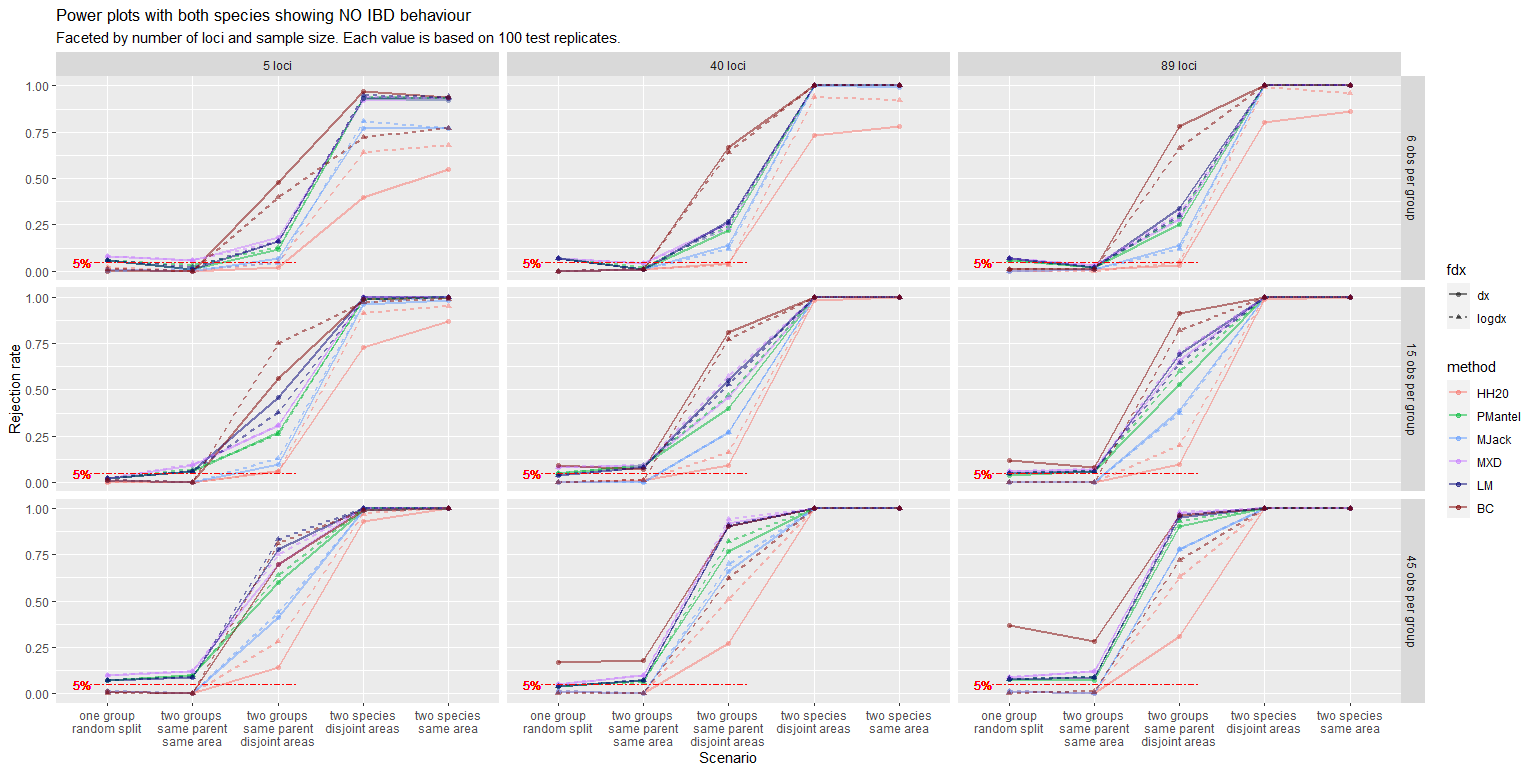
Figure 4.1: Power plot based on SLiM data simulated without IBD behaviour. Facets by number of individuals per group (rows) and number of available loci (columns). Each rejection rate is based on 100 simulations with same parameter settings. Circles and solid lines refer to analyses with untransformed geographic distances, whereas triangles and dashed lines refer to analyses with log-transformed ones. The horizontal dashed red line is superimposed to help assess type-I-error rates. HH20 is the protocol by [25]; PMantel is PMT with permutations; MJack is PMT with jackknife; BC is PMT with bias-corrected bootstrap; MXD is the extension to the model by [13]; LM is the multiple regression neglecting dependence.

In Figure 4.1, rejection rates from the scenarios with quasi-panmictic groups are reported (methods’ abbreviations are explained in the caption). The expected non-decreasing trend in the rejection rates was confirmed, with some minor exceptions between the split and the overlapping conspecific (same parent, same area) scenario. In the split scenario, all methods (surprisingly, model (3.16), too) displayed a type-I-error rate close to the significance level ($5\%$), although the bias-corrected bootstrap with untransformed $\mathbf{D}_{x}$ rejected the null hypothesis of conspecificity too often as the available information increased. More precisely, jackknife-based methods (HH20, MJack) showed type-I-error rates very close to zero, whereas all other methods lay slightly above the significance threshold. In the second scenario, especially with large samples, these methods showed rejection rates close to $10\%$.
In the separated conspecific (same parent, disjoint areas) scenario, all rejection rates registered a strong increase: especially with many individuals and loci, all methods seemed to suggest that the two groups should be considered distinct, despite having originated from the same parent population. This was probably due to the combination of geographic separation and absence of IBD behaviour: the genetic structure that was formed because of the decreasing migration rate could not be explained by geographic distance as individuals in the same group tended to be quasi-panmictic. It can be controversial whether the groups generated with this particular SLiM script should be considered conspecific: most methods concluded they are not.
Under the multispecies setups, all methods displayed a rejection rate close to 1, especially in less demanding data scenarios. Jackknife-based methods, though, tended to display lower power with respect to the other methods, particularly with small sample sizes. This trend was common to all scenarios: PMantel, MXD, LM and BC always showed rejection rates larger than HH20 and MJack. In this respect, it is worth noting that MJack, representing a compromise between HH20 and PMantel, displayed satisfactory type-I-error rate and larger power than HH20 in all setups. Now, if the rejection of the null hypothesis in the split scenario is seen as a Bernoulli random variable with success probability equal to $0.05$, 10 rejections out of 100 would represent a significant result (if again a significance level of $5\%$ for the binomial test is considered): PMantel did not consistently display such significant figures in the simulations, but in an ad hoc simulation under the null hypothesis, with $15$ individuals per group and $40$ loci (not shown here), this test rejected 70 times out of 1000 repetitions (one-sided p-value $=0.0023$ against the null hypothesis that the rejection probability is 0.05). By replacing the permutation-based significance assessment with a jackknife-based one, MJack achieved more power than HH20 while keeping its same low type-I-error rate. This might support the idea that permutations introduce a distortion in the distribution of geographic distances.

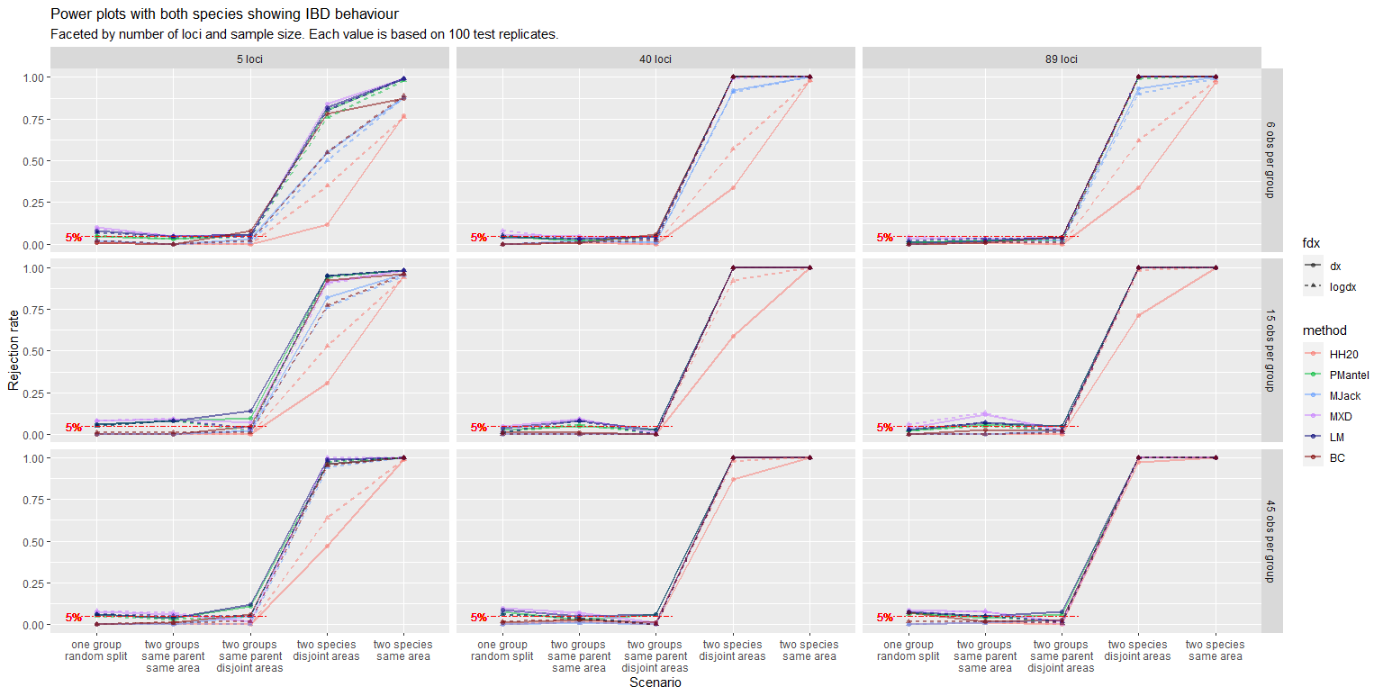
Figure 4.2: Power plot based on SLiM data simulated with IBD behaviour. See the caption to Figure 4.1 for further description.

Also in Figure 4.2, with isolated by distance individuals, the rejection rates were mostly non-decreasing when going from the split scenario to the overlapping distinct scenario. There were no remarkable differences between data analyses with or without the transformation of the geographic distances, as with quasi-panmictic groups. The only exception is HH20, whose power increased with log-transformed geographic dissimilarities. The two multispecies setups did not imply different performances in terms of power.
The most remarkable difference among the two charts relates the separated conspecific scenario, since with IBD species the rejection rates dropped to values close to the significance level: here, the tendency of individuals to be more genetically diverse within group was able to explain the differences between the groups, too, causing all methods not to reject the null hypothesis of conspecificity in most cases.

4.1.2 The GSpace software [67]

As clarified in its user manual [66], GSpace is a a backward generation by generation exact coalescence algorithm with recombination that allows to simulate allelic data on a lattice under isolation by distance. Each deme on the lattice can represent the locality in population-level simulations or the position of single individuals on the map, approximating continuous habitats. Given the sampled individuals, the history of neutral genes is generated going backward in time and then mutations are simulated from the most recent common ancestor starting from the top of the coalescence tree down to the branches. At each generation, migration is handled by means of two-dimensional dispersal distributions, to be chosen among uniform, geometric, Zeta, etc. Details can be found in [31].
As far as the specific settings for the simulations carried out in this study are concerned, a $200\times 200$ demes map was created, with diploid individuals always inhabiting the central $60\times 60$ area. A first group would inhabit the area between point $(70,70)$ and point $(90,90)$, whereas a second group would inhabit the square between points $(110,110)$ and $(130,130)$. Their coordinates were drawn uniformly within the allowed range. A sequence of di-allelic loci was simulated, with both the mutation rate per generation per locus and the recombination rate per generation between loci equal to $0.005$ (ten times the default) for all simulated loci. The so-called K-allele mutation model was used, according to which the initial allelic state is changed into one of the other possible states - in this case the only other allele allowed in the di-allelic setting. In order to mimic a continuous habitat, in each deme there could be up to one individual.
In addition to this, the following parameters varied according to the scenario:

• in order to obtain a baseline scenario where the conspecificity hypothesis was trivially true, the two groups were simulated within the same software execution, so that the algorithm would reconstruct a unique genealogy common to all individuals. In all other cases, the two geographically separated groups were generated during two distinct software executions and collected in the same dataset.

• The two groups would obviously share the same allele pools (the same two allele options for all loci) when generated within the same software execution, whereas they could share both alleles, one allele or no allele otherwise. Of course, when no allele was shared, the genetic dissimilarities between individuals from different groups would always take value one.

• IBD behaviour was controlled via the choice of the univariate dispersal distribution: GSpace assumes that dispersal occurs independently in each dimension. In order to yield panmictic groups, a uniform dispersal was used, according to which the probability of moving $t$ steps in one direction is $\frac{m}{d_{max}}$, where $m$ is the total migration rate, equal to $0.5$ and $d_{max}$ is the maximum distance reachable in any migration event, set to $200$ (the largest possible value) in all scenarios. As regards IBD species, a Zeta (or truncated discrete Pareto) dispersal distribution was used, assigning value $\frac{m}{2{|t|}^{\kappa}}$ to the probability to move $t$ steps in one direction, with $\kappa=5$ being the shape parameter.

• The number of individuals simulated per group was either $6$, $15$ or $45$, whereas the genetic sequence was either $4$, $40$ or $100$ loci long.

The script on which these simulations were based and distance-distance plots from all simulated scenarios can be found in Appendix A.

Results from GSpace

The combination of the parameter settings illustrated above led to a total of four scenarios: the simulation involving a unique software execution represented a conspecificity setup, whereas the situation where the allele pools of the two groups shared no allele constituted a distinctness one. The other two setups were included as intermediate situations, with the two groups not sharing ancestors while still showing similarities in their genetic information. Recall that in all these scenarios, the geographic separation was always the same: the two groups inhabited two disjoint areas of the map. The four scenarios can be sorted as follows: one execution (split), two executions and same alleles (same allele pool), two executions and one allele in common (overlapping allele pools), two executions and no allele in common (disjoint allele pools). In this order, the rejection rate is expected to be non-decreasing.
On top of these scenarios, other varying parameters were the number of individuals per group, the number of loci available for the analysis and the IBD behaviour (absent with Uniform dispersal distribution and strong with Zeta dispersal distribution). Each of these parameter (and scenario) combinations was simulated one hundred times and the number of rejections was recorded. This data is displayed in the following power plots, one per IBD behaviour.

Figure 4.3: Power plot based on GSpace data simulated without IBD behaviour. See the caption to Figure 4.1 for further description.

In Figure 4.3 the results related to species without IBD behaviour are reported. It is apparent how the ranking of the methods in terms of performance was similar to that observed in SLiM, apart from the odd behaviour of BC, which displayed very large type-I-error rates especially with fewer loci and fewer individuals: this is probably due to the emergence of too many null dissimilarities during the bootstrap resampling, which would invalidate the computation of the partial correlation coefficients needed for the test. Jackknife-based methods showed lower power with respect to other methods and once again the logarithmic transformation of $\mathbf{D}_{x}$ helped HH20 be more powerful. Differences among methods were only detectable in the most challenging data scenarios.

Figure 4.4: Power plot based on GSpace data simulated with IBD behaviour. Facets by number of individuals per group (rows) and number of available loci (columns). See the caption to Figure 4.1 for further description.

As shown in Figure 4.4, the rejection rates of the methods with IBD groups were more various. Bootstrap-based PMT displayed again unacceptable type-I-error rates, while the multiple regression neglecting dependence confirmed its outstanding performance both in terms of type-I-error and in terms of power, especially with log-transformed geographic dissimilarities. Also with GSpace, MJack showed more power than HH20 and similar type-I-error rate, whereas PMantel had type-I-error rates sometimes slightly above the significance threshold.

4.2 Discussion

The individual-based spatially-explicit simulations carried out via SLiM [21] and GSpace [67] allowed to study the type-I-error rate and power of the techniques described in the Methods section. A consistent ranking in the overall performance of the methodologies could be observed, with jackknife-based methods being very conservative and not very powerful and the other techniques being more powerful, sometimes at the cost of empirical type-I-error rates consistently above the significance level.
By combining jackknife significance assessment and the usage of partial correlation coefficients, MJack managed to achieve larger power with respect to HH20, while showing type-I-error rates consistently beneath the significance level, unlike PMantel. Bias-corrected bootstrap-based PMT showed a large type-I-error rate in the most challenging data setups. No method apart from HH20 clearly benefited from the logarithmic transformation of the geographic distances.
Despite assuming that all dissimilarities in the dataset are independent, model (3.16) displayed one of the best performances, both in terms of type-I-error rate and power. Results suggest that this multiple linear regression did not underestimate the variability of the $\beta^{*}_{2}$ parameter associated with the grouping distance and could detect evidence for distinctness, in terms of increased overall genetic structure after controlling for geographic separation, more accurately than PMT or MXD. It is not clear why relying on an inflated sample size ($w$ instead of the effective number of individuals $n$) did not imply inflated type-I-error, but the slight superiority of LM with respect to MXD might be due to the instability of maximum likelihood estimation compared to OLS, given that the the dependence structure is possibly misspecified in MXD: the model by [13] (and its extension used here) assumes individual-specific intercept updates to the relationship between genetic and geographic dissimilarities, regardless of the grouping. It could be argued that the random intercept associated with a given individual should change according to the comparison being within or between groups, albeit this information might already be successfully modeled by the grouping fixed effect.
The performance of the protocol by [25] had to be summarized with a unique rejection rate to be shown in the power plots, but it is crucial to recall that this methodology is hierarchical: in this study, a rejection corresponded to cases when either $H_{02}$ or $H_{03}$ was rejected (the latter implying a rejection of both sub-tests) and thus, in that summary, a non-rejection included also the inconclusive results that can arise when testing $H_{03}$. Although in all simulations both groups always had the same IBD behaviour, some rejections of $H_{01}$ occurred, leading the protocol towards a test for $H_{03}$: on one hand, this might have led to lower displayed rejection rates in the power plots in spite of the fact that, in some unclear cases, a practitioner could have concluded that two distinct species were being compared; on the other hand, the possibility to take into consideration unequal IBD behaviour is unique to HH20, but here could only degrade its performance by introducing complexity, while all other methods assumed equal IBD behaviour - consistently with what was being simulated.

5 Real data analysis

5.1 Brassy Ringlets (Erebia tyndarus complex, Lepidoptera)

[20] discussed the biological delimitation of a taxon of butterflies endemic to Southern Europe, the Altai Republic and the Rocky Mountains by studying the morphological, genetic and geographic information of $45$ individuals netted during the summer of 2012 across the Italian Appennines, the Alps and the Pyrenees. Four subgroups of this clade were represented in the sample, namely E. Tyndarus, E. Nivalis, E. Calcaria and E. Cassioides, with the latter possibly divisible in three populations according to the area of collection. After selecting a subset of $389$ diploid loci, they applied k-means clustering on the principal components obtained from the genetic data, Bayesian model-based clustering using the STRUCTURE software [46] and coalescent-based Bayes factor delimitation [30], integrating their results by examining the isolation by distance behaviour and morphological differentiation of the individuals in each putative cluster. The details can be found in [20]: their study not only backed up the distinction in the four groups mentioned above from a genetic point of view, but also supported the further classification, within the Cassioides group, among the Eastern and Orobian Alps population, the Southern and Central Appennines population and the population inhabiting Northern Appennines, Pyrenees and Western Alps.
[25] applied their testing protocol to this data in order to replicate and deepen the IBD investigation carried out by [20]. With the exclusion of the Calcaria group, which could not be examined due to the small sample size (only $3$ specimens), the distinction among the groups was confirmed. The classification within the Cassioides group, instead, was slightly amended: their method suggested that there was no evidence of distinctness between the Southern and Central Appennines population and the population inhabiting Northern Appennines, Pyrenees and Western Alps, whereas the genetic dissimilarity between these populations taken together and the Eastern and Orobian Alps population was too large to be explained by isolation by distance.

Table 1: Results from all methods (see abbreviations in Figure 4.1) compared in this study on the data by [20]. For the three tests in HH20, the p-value is reported (two of them are specified for $H_{03}$ when discordant); p-values are reported for PMantel, MJack and LM, too; for MXD and BC, confidence intervals are reported for the $\beta_{2}^{*}$ regression coefficient and the partial correlation coefficient, respectively: if their lower boundary is larger than zero, the null hypothesis is rejected.

Groups compared	$H_{01}$	$H_{02}$	$H_{03}$	PMantel	MJack	MXD	LM	BC
E. Tyndarus vs E. Nivalis	$0.074$	$<10^{-5}$	n.a.	$0.001$	$<10^{-29}$	$(0.296,0.306)$	$<10^{-113}$	$(0.983,0.995)$
E. Nivalis vs E. Cassioides	$0.094$	$<10^{-4}$	n.a.	$0.001$	$<10^{-55}$	$(0.378,0.389)$	$\sim 0$	$(0.972,0.988)$
E. Tyndarus vs E. Cassioides	$<10^{-9}$	n.a.	$\text{both}<10^{-24}$	$0.001$	$<10^{-67}$	$(0.345,0.352)$	$\sim 0$	$(0.977,0.986)$
E. Cassioides: W_Alps + Pyrenees + N_Apennines vs Orobian + E_Alps	$0.487$	$0.004$	n.a.	$0.001$	$<10^{-5}$	$(0.025,0.036)$	$<10^{-17}$	$(0.493,0.745)$
E. Cassioides: W_Alps + Pyrenees + N_Apennines vs Central + S_Apennines	$<10^{-4}$	n.a.	$0.098;0.004$	$0.002$	$0.015$	$(0.030,0.045)$	$<10^{-5}$	$(-0.148,0.552)$
E. Cassioides: Central + S_Apennines vs Orobian + E_Alps	$0.144$	$0.009$	n.a.	$0.001$	$<10^{-4}$	$(0.041,0.066)$	$<10^{-15}$	$(0.477,0.484)$
E. Cassioides: W_Alps + Pyrenees + ALL Apennines vs Orobian + E_Alps	$1$	$<10^{-4}$	n.a.	$0.001$	$<10^{-8}$	$(0.020,0.029)$	$<10^{-25}$	$(0.329,0.618)$

In Table 1, the results from all methods involved in this study applied on the data by [20] are reported. The results reported by [25] were reproducible almost everywhere, although the comparison between the individuals from Southern and Central Appennines population and the population inhabiting Northern Appennines, Pyrenees and Western Alps led to discordant p-values when testing $H_{03}$ (this term is used here to mean that one p-value was lower than the significance threshold and one larger; concordant p-values are either both below or above the threshold). The authors only showed the largest of the p-values in the supplementary material to their paper, clarifying that the other would be omitted if concordant (in this case, this would mean that also the other p-value was larger than $5\%$ in their analysis - whereas here it was equal to $0.004$). In their paper, the authors concluded that the data provide no evidence for the specific distinctness of these two subgroups, which would be the logical conclusion if both of the aforementioned p-values were larger than the significance level. In this study, however, the only failure to reject the null hypothesis of conspecificity was returned by the bias-corrected bootstrap-based Partial Mantel test (the CI contains $0$), whereas all other methods rejected it: in particular, the p-value from the model neglecting dependence was very small ($<10^{-5}$).
In all other cases, all methods agreed upon the distinctness results, confirming the conclusions shared by [20] and [25] - including also the distinction between the Western and Appennines populations versus the Eastern and Orobian populations (last row in Table 1). According to the evidence collected in this study, not only the E. Tyndarus, E. Nivalis and E. Cassioides groups should be considered distinct: also the three subgroups identified within the E. Cassioides group, namely the Eastern and Orobian Alps population, the Southern and Central Appennines population and the population inhabiting Northern Appennines, Pyrenees and Western Alps, display a genetic structure that cannot be explained by their geographic separation. Anyway, as already suggested in the two cited papers, further investigation is required to confirm these findings, particularly aiming for larger sample sizes (and more specimens from the E. Calcaria group).

6 Conclusions

This paper investigated methods that model the relationship between genetic and geographic dissimilarities in biological species in order to perform species delimitation. These techniques check whether the genetic structure existing between two putative species is compatible with the way genetic dissimilarities within each group increase with the geographic separation of the individuals. The type-I-error rate and power of these methods were compared by means of individual-based simulations carried out with GSpace [67] and SLiM [21]. Results showed that the protocol by [25] has type-I-error rate close to zero and lower power than Partial Mantel tests (PMTs) as applied by [41], which in turn had type-I-error rates above the significance level in some setups. Testing PMTs with jackknife instead of permutations fixed this behaviour, ensuring more power than the protocol by [25] while keeping the type-I-error rate still close to zero. Testing PMTs with bias-corrected bootstrap confidence intervals, instead, often led to inflated type-I-error rates. The linear mixed model proposed by [13], with an extension for species delimitation, displayed a performance similar to PMT, while its nested version without random effects (i.e., a multiple regression assuming independence among the dissimilarities) surprisingly did not show inflated type-I-error rates. It is not clear why neglecting the dependence intrinsic to the dissimilarities and assuming a sample size larger than the effective one did not imply an underestimation of the variability of the estimate of the parameter associated with the grouping distance in such model. This behaviour has to be investigated further. The ranking in the overall performance of the methods was confirmed by both simulation packages and the log-transformation of the geographic dissimilarities did not seem to have a considerable impact.
For further research, additional simulations could be considered. Some scenarios worth exploring could involve comparisons between groups with different IBD behaviour, sample size or size (and separation) of the inhabited areas, but also simulations with independent loci, different settings for the time scale and migration rates, etc. Moreover, the investigation carried out in this study could be extended to population-based simulations, using genetic dissimilarity measures like $F_{st}$ [69] or the chord distance [11]. The individual-based methods compared in this study often assume independence between observations in the same group, something that is not biologically grounded and is indeed avoided in population-based studies.
In addition, another simulation-based investigation could be set up in order to compare the performance of these methods in scenarios where there is no known putative grouping. In this direction, an automated clustering routine may be conceived, that would be comparable with conStruct [8], a method that only works in an unsupervised way, and could even complement its area of application given that conStruct is only applicable when the number of loci is much larger than $n$ (whereas, as shown in this study, most methods investigated here worked fairly good even with very small $n$ and $P$).

Appendix A Software code and distance-distance plots

A.1 SLiM

Script editing, software executions and data analysis were carried out in R. The variables defined with the defineConstant command were set at each simulation iteration before feeding the script to the SLiM executable: for instance, nsam would take value $6$, $15$ or $45$ according to the scenario at hand.

Listing 1: SLiM script for the split scenario

⬇

1initialize() {

2initializeSLiMOptions(keepPedigrees = T, dimensionality="xy", nucleotideBased=T);

3 defineConstant("L", 1e3);

4 initializeAncestralNucleotides(randomNucleotides(L));

5 initializeMutationTypeNuc("m1", 0.5, "f", 0.0);

6 initializeGenomicElementType("g1", m1, 1.0, mmJukesCantor(2.5e-3));

7 initializeGenomicElement(g1, 0, L-1);

8 initializeRecombinationRate(rates = 1e-8);

9

10 defineConstant(symbol="nsim", value=200);

11 defineConstant(symbol="nsam", value=45);

12 defineConstant(symbol="i1sd", value=1);

13 defineConstant(symbol="i2maxd", value=3);

14 defineConstant(symbol="nneigh", value=3);

15 defineConstant(symbol="childsd", value=9);

16

17 // spatial competition

18 initializeInteractionType(1, "xy", reciprocal=T, maxDistance=3*i1sd);

19 i1.setInteractionFunction("n", i1sd/2, i1sd);

20

21

22 // spatial mate choice

23 initializeInteractionType(2, "xy", reciprocal=T, maxDistance=i2maxd);

24}

25

261 late() {

27 sim.addSubpop("p0", nsim*2);

28 p0.setSpatialBounds(c(50.00, 50.00, 150.00, 150.00));

29 p0.individuals.setSpatialPosition(p0.pointUniform(nsim*2));

30}

31

321:100 late() {

33 i1.evaluate(p0);

34 inds = p0.individuals;

35 competition = i1.totalOfNeighborStrengths(inds) / size(inds);

36 competition = pmin(competition, 0.99);

37 inds.fitnessScaling = 1 - competition;

38}

39

402:100 first() {

41 i2.evaluate(p0);

42}

43

44mateChoice(p0) {

45 // nearest-neighbor mate choice

46 neighbors = i2.nearestNeighbors(individual, count = nneigh);

47 return (size(neighbors) ? sample(neighbors, 1) else float(0));

48}

49modifyChild(p0) {

50 do pos = parent1.spatialPosition + rnorm(2, 0, childsd);

51 while (!p0.pointInBounds(pos));

52 child.setSpatialPosition(pos);

53

54 return T;

55}

56

57100 late() { // last generation

58 sampledIndividuals = p0.sampleIndividuals(nsam*2);

59

60 out = paste("subpopulation", "pedigreeID", "x", "y", "genome1", "genome2");

61 for (i in sampledIndividuals){

62 info = paste(i.subpopulation, i.pedigreeID, i.spatialPosition, i.genome1.nucleotides(), i.genome2.nucleotides());

63 out = c(out, info);

64 }

65 writeFile("coordgenomes.txt", out);

66}

Listing 2: SLiM script for the conspecificity scenario

⬇

1initialize() {

2 initializeSLiMOptions(keepPedigrees = T, dimensionality="xy", nucleotideBased=T);

3 defineConstant("L", 1e3);

4 initializeAncestralNucleotides(randomNucleotides(L));

5 initializeMutationTypeNuc("m1", 0.5, "f", 0.0);

6 initializeGenomicElementType("g1", m1, 1.0, mmJukesCantor(2.5e-3));

7 initializeGenomicElement(g1, 0, L-1);

8 initializeRecombinationRate(rates = 1e-8);

9

10 defineConstant(symbol="nsim", value=200);

11 defineConstant(symbol="nsam", value=45);

12 defineConstant(symbol="i1sd", value=1);

13 defineConstant(symbol="i2maxd", value=3);

14 defineConstant(symbol="nneigh", value=3);

15 defineConstant(symbol="childsd", value=9);

16 defineConstant(symbol="separation", value=F);

17

18 // spatial competition

19 initializeInteractionType(1, "xy", reciprocal=T, maxDistance=3*i1sd);

20 i1.setInteractionFunction("n", i1sd/2, i1sd);

21

22 // spatial mate choice

23 initializeInteractionType(2, "xy", reciprocal=T, maxDistance=i2maxd);

24}

251 late() {

26 sim.addSubpop("p0", nsim*2);

27 p0.setSpatialBounds(c(50.00, 50.00, 150.00, 150.00));

28 p0.individuals.setSpatialPosition(p0.pointUniform(nsim*2));

29}

30

311:100 late() {

32 i1.evaluate(p0);

33 inds = p0.individuals;

34 competition = i1.totalOfNeighborStrengths(inds) / size(inds);

35 competition = pmin(competition, 0.99);

36 inds.fitnessScaling = 1 - competition;

37}

382:100 first() { i2.evaluate(p0); }

39

4090 early() {

41 sim.addSubpopSplit("p1", nsim, p0);

42 sim.addSubpopSplit("p2", nsim, p0);

43 p1.setSpatialBounds(c(50.00, 50.00, 150.00, 150.00));

44 p2.setSpatialBounds(c(50.00, 50.00, 150.00, 150.00));

45 p1.individuals.setSpatialPosition(p1.pointUniform(nsim));

46 p2.individuals.setSpatialPosition(p2.pointUniform(nsim));

47}

48

4991: late() {

50 i1.evaluate(p1);

51 inds = p1.individuals;

52 competition = i1.totalOfNeighborStrengths(inds) / size(inds);

53 competition = pmin(competition, 0.99);

54 inds.fitnessScaling = 1 - competition;

55

56 i1.evaluate(p2);

57 inds = p2.individuals;

58 competition = i1.totalOfNeighborStrengths(inds) / size(inds);

59 competition = pmin(competition, 0.99);

60 inds.fitnessScaling = 1 - competition;

61}

62

6392: first() {

64 i2.evaluate(p1);

65 i2.evaluate(p2);

66}

67

68101 early() { p0.setSubpopulationSize(0); }

69

70

71101:150 early() {

72 if(separation){

73p1.setSpatialBounds(p1.spatialBounds + c(0, 0, -1, -1));

74p2.setSpatialBounds(p2.spatialBounds + c(1, 1, 0, 0));

75 }

76}

77

7892: early() {

79 migrationProgress = runif(1, min=0.8, max=1);

80 p1.setMigrationRates(p2, 0.5 * migrationProgress);

81 p2.setMigrationRates(p1, 0.5 * migrationProgress);

82}

83

84

85// NEAREST NEIGHBORS MATE CHOICE

862:91 mateChoice(p0) {

87 // nearest-neighbor mate choice

88 neighbors = i2.nearestNeighbors(individual, count = nneigh);

89 return (size(neighbors) ? sample(neighbors, 1) else float(0));

90}

912:91 modifyChild(p0) {

92 do pos = parent1.spatialPosition + rnorm(2, 0, childsd);

93 while (!p0.pointInBounds(pos));

94 child.setSpatialPosition(pos);

95 return T;

96}

97

9892: mateChoice(p1) {

99 // nearest-neighbor mate choice

100 neighbors = i2.nearestNeighbors(individual, count = nneigh);

101 return (size(neighbors) ? sample(neighbors, 1) else float(0));

102}

10392: mateChoice(p2) {

104 // nearest-neighbor mate choice

105 neighbors = i2.nearestNeighbors(individual, count = nneigh);

106 return (size(neighbors) ? sample(neighbors, 1) else float(0));

107}

108

10992: modifyChild(p1) {

110 counter = 1;

111 do{

112 pos = parent1.spatialPosition + rnorm(2, ifelse(separation, -0.5, 0.0), childsd);

113 counter = counter + 1;

114 }

115 while (!p1.pointInBounds(pos) & counter < 100);

116 child.setSpatialPosition(pos);

117 return T;

118}

11992: modifyChild(p2) {

120 counter = 1;

121 do{

122 pos = parent1.spatialPosition + rnorm(2, ifelse(separation, 0.5, 0.0), childsd);

123 counter = counter + 1;

124 }

125 while (!p2.pointInBounds(pos) & counter < 100);

126 child.setSpatialPosition(pos);

127 return T;

128}

129150 late() { // last generation

130 allind1 = p1.individuals[p1.pointInBounds(p1.individuals.spatialPosition)];

131 allind2 = p2.individuals[p2.pointInBounds(p2.individuals.spatialPosition)];

132 sampledIndividuals = c(sample(allind1, nsam), sample(allind2, nsam));

133 sampledIndividuals.genomes.outputVCF(filePath="tmp.VCF", outputMultiallelics = F, simplifyNucleotides=T);

134

135 out = paste("subpopulation", "pedigreeID", "x", "y", "genome1", "genome2");

136 for (i in sampledIndividuals){

137 info = paste(i.subpopulation, i.pedigreeID, i.spatialPosition, i.genome1.nucleotides(), i.genome2.nucleotides());

138 out = c(out, info);

139 }

140 writeFile("coordgenomes.txt", out);

141}

Listing 3: SLiM script for the distinctness scenario

⬇

1species all initialize() {

2 defineConstant("L", 1e3);

3 defineConstant(symbol="nsim", value=200);

4 defineConstant(symbol="nsam", value=45);

5 defineConstant(symbol="i1sd", value=1);

6 defineConstant(symbol="i2maxd", value=3);

7 defineConstant(symbol="nneigh", value=3);

8 defineConstant(symbol="childsd", value=9);

9

10 // spatial competition

11 initializeInteractionType(1, "xy", reciprocal=T, maxDistance=3*i1sd);

12 i1.setInteractionFunction("n", i1sd/2, i1sd);

13

14 // spatial mate choice

15 initializeInteractionType(2, "xy", reciprocal=T, maxDistance=i2maxd);

16}

17

18species sunflower initialize() {

19 initializeSpecies(tickModulo=1, tickPhase=1, avatar="S");

20 initializeSLiMOptions(keepPedigrees = T, dimensionality="xy", nucleotideBased=T);

21 initializeAncestralNucleotides(randomNucleotides(L, c(1, 1, 1, 1)));

22 initializeMutationTypeNuc("m1", 0.5, "f", 0.0);

23 initializeGenomicElementType("g1", m1, 1.0, mmJukesCantor(2.5e-3));

24 initializeGenomicElement(g1, 0, L-1);

25 initializeRecombinationRate(rates = 1e-8);

26}

27

28species tulip initialize() {

29 initializeSpecies(tickModulo=1, tickPhase=1, avatar="T");

30 initializeSLiMOptions(keepPedigrees = T, dimensionality="xy", nucleotideBased=T);

31 initializeAncestralNucleotides(randomNucleotides(L, c(1, 1, 1, 1)));

32 initializeMutationTypeNuc("m2", 0.5, "f", 0.0);

33 initializeGenomicElementType("g2", m2, 1.0, mmJukesCantor(2.5e-3));

34 initializeGenomicElement(g2, 0, L-1);

35 initializeRecombinationRate(rates = 1e-8);

36}

37

38ticks all 1 early() {

39 sunflower.addSubpop("p1", nsim);

40 tulip.addSubpop("p2", nsim);

41 p1.setSpatialBounds(c(50.00, 50.00, 100.00, 100.00));

42 p2.setSpatialBounds(c(100.00, 100.00, 150.00, 150.00));

43 p1.individuals.setSpatialPosition(p1.pointUniform(nsim));

44 p2.individuals.setSpatialPosition(p2.pointUniform(nsim));

45}

46

47ticks all 1: late() {

48 i1.evaluate(p1);

49 inds = p1.individuals;

50 competition = i1.totalOfNeighborStrengths(inds) / size(inds);

51 competition = pmin(competition, 0.99);

52 inds.fitnessScaling = 1 - competition;

53

54 i1.evaluate(p2);

55 inds = p2.individuals;

56 competition = i1.totalOfNeighborStrengths(inds) / size(inds);

57 competition = pmin(competition, 0.99);

58 inds.fitnessScaling = 1 - competition;

59}

60

61ticks all 2: first() {

62 i2.evaluate(p1);

63 i2.evaluate(p2);

64}

65

66// NEAREST NEIGHBORS MATE CHOICE

67species sunflower 2: mateChoice(p1) {

68 // nearest-neighbor mate choice

69 neighbors = i2.nearestNeighbors(individual, count = nneigh);

70 return (size(neighbors) ? sample(neighbors, 1) else float(0));

71}

72species tulip 2: mateChoice(p2) {

73 // nearest-neighbor mate choice

74 neighbors = i2.nearestNeighbors(individual, count = nneigh);

75 return (size(neighbors) ? sample(neighbors, 1) else float(0));

76}

77species sunflower modifyChild(p1) {

78 do pos = parent1.spatialPosition + rnorm(2, 0, childsd);

79 while (!p1.pointInBounds(pos));

80 child.setSpatialPosition(pos);

81

82 return T;

83}

84species tulip modifyChild(p2) {

85 do pos = parent1.spatialPosition + rnorm(2, 0, childsd);

86 while (!p2.pointInBounds(pos));

87 child.setSpatialPosition(pos);

88

89 return T;

90}

91

92ticks all 50 late() { // last generation

93 allind1 = p1.individuals;

94 allind2 = p2.individuals;

95 sampled1 = sample(allind1, nsam);

96 sampled2 = sample(allind2, nsam);

97 sampledIndividuals = c(sampled1, sampled2);

98

99 out = paste("subpopulation", "pedigreeID", "x", "y", "genome1", "genome2");

100 for (i in sampledIndividuals){

101 info = paste(i.subpopulation, i.pedigreeID, i.spatialPosition, i.genome1.nucleotides(), i.genome2.nucleotides());

102 out = c(out, info);

103 }

104 writeFile("coordgenomes.txt", out);

105}

Figure A.1: Distance-distance plots (shared allele distance against log-transformed geographic distance) from the five scenarios simulated with SLiM, without IBD behaviour, $15$ individuals per group and $40$ available loci. Each scenario is specified in the plot title. In black the dissimilarities among individuals belonging to the first group, in red those for the second group and in green the dissimilarities among individuals belonging to different groups.

In Figure A.1, the shared allele distance is plotted against the log-transformed geographic distance for a random dataset from each of the five scenarios simulated by SLiM without IBD behaviour. It is easy to see that, by colour, there was no association between genetic and geographic dissimilarities. The split and the overlapping conspecific scenarios are similar, with the latter displaying a larger variability in the genetic dissimilarities. In the third scenario, the geographic separation can be clearly seen by the range of the green-colored points. In the multispecies scenarios (bottom row), the range of the between-group genetic dissimilarities was always above that of the within-group ones, supporting distinctness: models that fit an update in the intercept to a linear regression of $\mathbf{D}_{y}$ against $\mathbf{D}_{x}$ easily caught this trend in the data.

Figure A.2: Distance-distance plots (shared allele distance against log-transformed geographic distance) from the five scenarios simulated with SLiM, with IBD behaviour, $15$ individuals per group and $40$ available loci. Each scenario is specified in the plot title. In black the dissimilarities among individuals belonging to the first group, in red those for the second group and in green the dissimilarities among individuals belonging to different groups.

In Figure A.2, the same kind of plots are shown for IBD species. It is apparent how the shared allele distance is positively correlated with geographic distance as far as individuals close in space are considered, but this trend soon plateaus and dissimilarities never take values larger than around $0.9$ (also in the quasi-panmictic datasets). This saturation causes a convexity in the relationship that is not fixed by the logarithmic transformation of the geographic distances. Also in this chart it is easy to notice: a) how within and between-group dissimilarities are separated in the distinct scenarios and b) how the IBD behaviour is common to both groups.

A.2 GSpace

Script editing, software executions and data analysis were carried out in R. Variables like Sequence_Size or Dispersal_Distribution were modified according to the scenario at hand.
When only one software execution was involved (trivial conspecificity scenario), all individuals from the two groups were simulated at once, using a longer sequence of random coordinates next to the Sample_Coordinate variables. In all other situations, the code was run twice with half that number of coordinate pairs, each time fulfilling the geographic separation explained in section 4.1.2: e.g., individuals from the first group would have coordinates bound within point $(70,70)$ and point $(90,90)$.

Listing 4: Common structure of the GSpace script

⬇

1%%%%%%%% SIMULATION SETTINGS %%%%%%%%%%%%%%%

2Setting_Filename = GSpaceSettings.txt

3Random_seeds = 11000

4Run_Number = 1

5

6%%%%%%%% OUTPUT FILE FORMAT SETTINGS %%%%%%%

7Output_Dir = .

8Data_File_Name = trial

9Data_File_Extension = .txt

10

11Genepop = True

12Genepop_ind_file = F

13Genepop_Group_All_Samples = T

14

15Approximate_time = F

16

17%%%%%%%% MARKERS SETTINGS %%%%%%%%%%%%%%%%%%

18Ploidy = Diploid

19Chromosome_number = 1

20Mutation_Rate = 0.005

21Mutation_Model = KAM

22Allelic_Lower_Bound = 240

23Allelic_Upper_Bound = 241

24Sequence_Size = 100

25

26%%%%%%%% RECOMBINATION SETTINGS %%%%%%%%%%%%

27Recombination_Rate = 0.005

28

29%%%%%%%% DEMOGRAPHIC SETTINGS %%%%%%%%%%%%%%

30%% LATTICE

31Min_Sample_Coord_X = 50

32Min_Sample_Coord_Y = 50

33Lattice_Size_X = 200

34Lattice_Size_Y = 200

35Ind_Per_Node = 1

36

37%% DISPERSAL

38Dispersal_Distribution = p

39Pareto_Shape = 5

40

41Edge_Effects = circular

42Total_Emigration_Rate = 0.5

43Disp_Dist_Max = 200, 200

44

45%%%%%%%% SAMPLE SETTINGS %%%%%%%%%%%%%%%%%%%

46Sample_Coordinate_X = 82,84,70,82,75,71,115,127,130,122,128,124

47Sample_Coordinate_Y = 89,76,89,72,73,70,111,116,128,120,117,129

48

49% STATS

50Dist_Class_Nbr = 1

51Ind_Per_Node_Sampled = 1

52Pause = Never

Figure A.3: Distance-distance plots (shared allele distance against log-transformed geographic distance) from the four scenarios simulated with GSpace, without IBD behaviour, $15$ individuals per group and $40$ available loci. Each scenario is specified in the plot title. In black the dissimilarities among individuals belonging to the first group, in red those for the second group and in green the dissimilarities among individuals belonging to different groups.

Figure A.4: Distance-distance plots (shared allele distance against log-transformed geographic distance) from the four scenarios simulated with GSpace, with IBD behaviour, $15$ individuals per group and $40$ available loci. Each scenario is specified in the plot title. In black the dissimilarities among individuals belonging to the first group, in red those for the second group and in green the dissimilarities among individuals belonging to different groups.

In Figure A.3, the shared allele distance is plotted against the log-transformed geographic distance for a random dataset from each of the four scenarios simulated by GSpace without IBD behaviour. As expected, there is no association between genetic and geographic dissimilarities within the groups. The split and same allele pool scenarios look rather similar and a major difference with respect to SLiM distinctness setups lies in the range of the dissimilarities among individuals belonging to different groups: in the disjoint allele pool scenario, since the genetic make-ups in the two groups are completely different, all genetic dissimilarities take value $1$.
In Figure 4.4, the same visualizations are provided for species displaying a positive association between genetic and geographic dissimilarities. This relationship is however harder to spot with respect to SLiM simulations as it seems to relate only a small share of the individuals in the two groups. In both Figures, the between-group genetic dissimilarities in the overlapping allele pool scenario are centered around the value $0.75$, whereas in all scenarios the bulk of the within-group shared allele distances is centered at $0.5$. This vertical shift in the genetic dissimilarities, which is even stronger in the last scenario, could be quite effectively captured by an update in the intercept of the linear models fitted on this data.

References

- [1] F. Adriaensen et al. “The application of ‘least-cost’ modelling as a functional landscape model” In Landscape and Urban Planning 64.4, 2003, pp. 233–247 DOI: https://doi.org/10.1016/S0169-2046(02)00242-6
- [2] Corey Devin Anderson et al. “Considering spatial and temporal scale in landscape-genetic studies of gene flow” In Molecular ecology 19.17 Oxford, UK: Oxford, UK : Blackwell Publishing Ltd, 2010, pp. 3565–3575
- [3] Niko Balkenhol, Samuel Cushman and Andrew Storfer “Landscape Genetics: Concepts, Methods, Applications” In Landscape Genetics Newark: Wiley, 2015, pp. 1–264
- [4] Sonja Bamberger, Jie Xu and Bernhard Hausdorf “Evaluating Species Delimitation Methods in Radiations: The Land Snail Albinaria cretensis Complex on Crete” In Systematic Biology 71.2, 2021, pp. 439–460 DOI: 10.1093/sysbio/syab050
- [5] Douglas Bates, Martin Mächler, Ben Bolker and Steve Walker “Fitting Linear Mixed-Effects Models Using lme4” In Journal of Statistical Software 67.1, 2015, pp. 1–48 DOI: 10.18637/jss.v067.i01
- [6] Yann XC Bourgeois and Ben H Warren “An overview of current population genomics methods for the analysis of whole-genome resequencing data in eukaryotes” In Molecular Ecology 30.23 Wiley Online Library, 2021, pp. 6036–6071
- [7] A. Bowcock et al. “High resolution of human evolutionary trees with polymorphic microsatellites” In Nature (London) 368.6470 London: Nature Publishing, 1994, pp. 455–457
- [8] Gideon S. Bradburd, Graham M. Coop and Peter L. Ralph “Inferring Continuous and Discrete Population Genetic Structure Across Space” In Genetics 210.1, 2018, pp. 33–52 DOI: 10.1534/genetics.118.301333
- [9] Frank T. Burbrink and Sara Ruane “Contemporary Philosophy and Methods for Studying Speciation and Delimiting Species” In Ichthyology & Herpetology 109.3, 2021, pp. 874–894 DOI: 10.1643/h2020073
- [10] Bryan C Carstens, Tara A Pelletier, Noah M Reid and Jordan D Satler “How to fail at species delimitation” In Molecular ecology 22.17 Wiley Online Library, 2013, pp. 4369–4383
- [11] L L Cavalli-Sforza and A W Edwards “Phylogenetic analysis. Models and estimation procedures” In American journal of human genetics 19.3 Pt 1, 1967, pp. 233–257
- [12] Hugo Cayuela et al. “Demographic and genetic approaches to study dispersal in wild animal populations: A methodological review” In Molecular ecology 27.20 England: Wiley Subscription Services, Inc, 2018, pp. 3976–4010
- [13] Ralph T Clarke, Peter Rothery and Alan F Raybould “Confidence limits for regression relationships between distance matrices: estimating gene flow with distance” In Journal of Agricultural, Biological, and Environmental Statistics 7.3 Springer, 2002, pp. 361–372
- [14] Kevin De Queiroz “Species Concepts and Species Delimitation” In Systematic Biology 56.6, 2007, pp. 879–886 DOI: 10.1080/10635150701701083
- [15] Danielle L Edwards and L Lacey Knowles “Species detection and individual assignment in species delimitation: can integrative data increase efficacy?” In Proceedings of the Royal Society B: Biological Sciences 281.1777 The Royal Society, 2014, pp. 20132765
- [16] Bradley Efron and Robert J. Tibshirani “An introduction to the bootstrap” In An introduction to the bootstrap New York London: Chapman & Hall, 1993
- [17] Bryan K. Epperson et al. “Utility of computer simulations in landscape genetics” In Molecular Ecology 19.17, 2010, pp. 3549–3564 DOI: https://doi.org/10.1111/j.1365-294X.2010.04678.x
- [18] A.. Frantz et al. “Using spatial Bayesian methods to determine the genetic structure of a continuously distributed population: clusters or isolation by distance?” In Journal of Applied Ecology 46.2, 2009, pp. 493–505 DOI: https://doi.org/10.1111/j.1365-2664.2008.01606.x
- [19] Sarah C Goslee and Dean L Urban “The ecodist package for dissimilarity-based analysis of ecological data” In Journal of Statistical Software 22, 2007, pp. 1–19
- [20] Paolo Gratton et al. “Testing Classical Species Properties with Contemporary Data: How ”Bad Species” in the Brassy Ringlets (Erebia tyndarus complex, Lepidoptera) Turned Good” In Systematic biology 65.2 England: Oxford University Press, 2016, pp. 292–303
- [21] Benjamin C Haller and Philipp W Messer “SLiM 4: multispecies eco-evolutionary modeling” In The American Naturalist 201.5 The University of Chicago Press Chicago, IL, 2023, pp. E127–E139
- [22] Benjamin C. Haller and Philipp W. Messer “SLiM Manual” Accessed: 2023-12-07, https://messerlab.org/slim/, 2022
- [23] Bernhard Hausdorf “PROGRESS TOWARD A GENERAL SPECIES CONCEPT” In Evolution 65.4, 2011, pp. 923–931 DOI: 10.1111/j.1558-5646.2011.01231.x
- [24] Bernhard Hausdorf and Christian Hennig “Package ’prabclus’, version 2.3-2”, 2019 URL: https://CRAN.R-project.org/package=prabclus
- [25] Bernhard Hausdorf and Christian Hennig “Species delimitation and geography” In Molecular Ecology Resources 20.4, 2020, pp. 950–960 DOI: https://doi.org/10.1111/1755-0998.13184
- [26] Delbert W. Hutchison and Alan R. Templeton “Correlation of Pairwise Genetic and Geographic Distance Measures: Inferring the Relative Influences of Gene Flow and Drift on the Distribution of Genetic Variability” In Evolution 53.6 United States: Society for the Study of Evolution, 1999, pp. 1898–1914
- [27] Yoichi Ishida “Sewall Wright and Gustave Malécot on Isolation by Distance” In Philosophy of Science 76.5 [The University of Chicago Press, Philosophy of Science Association], 2009, pp. 784–796 URL: https://www.jstor.org/stable/10.1086/605802
- [28] Thomas H. Jukes and Charles R. Cantor “CHAPTER 24 - Evolution of Protein Molecules” In Mammalian Protein Metabolism Academic Press, 1969, pp. 21–132 DOI: https://doi.org/10.1016/B978-1-4832-3211-9.50009-7
- [29] Motoo Kimura and G.. Weiss “The Stepping Stone Model of Population Structure and the Decrease of Genetic Correlation with Distance” In Genetics (Austin) 49.4, 1964, pp. 561–576
- [30] Adam D. Leaché, Matthew K. Fujita, Vladimir N. Minin and Remco R. Bouckaert “Species Delimitation using Genome-Wide SNP Data” In Systematic biology 63.4 England: Oxford University Press, 2014, pp. 534–542
- [31] Raphaël Leblois, Arnaud Estoup and Francois Rousset “IBDSim: a computer program to simulate genotypic data under isolation by distance” In Molecular Ecology Resources 9.1 Wiley Online Library, 2009, pp. 107–109
- [32] Pierre Legendre “Comparison of permutation methods for the partial correlation and partial Mantel tests” In Journal of statistical computation and simulation 67.1 Taylor & Francis, 2000, pp. 37–73
- [33] Pierre Legendre and Marie-Josée Fortin “Comparison of the Mantel test and alternative approaches for detecting complex multivariate relationships in the spatial analysis of genetic data” In Molecular Ecology Resources 10.5, 2010, pp. 831–844 DOI: https://doi.org/10.1111/j.1755-0998.2010.02866.x
- [34] Pierre Legendre, Marie‐Josée Fortin, Daniel Borcard and Pedro Peres‐Neto “Should the Mantel test be used in spatial analysis?” In Methods in ecology and evolution 6.11 HOBOKEN: Wiley, 2015, pp. 1239–1247
- [35] Pierre Legendre and Louis Legendre “Numerical ecology”, Developments in environmental modelling ; 24 Amsterdam ; Boston: Elsevier, 2012
- [36] Zachary G. MacDonald et al. “Gene flow and climate-associated genetic variation in a vagile habitat specialist” In Molecular Ecology 29.20, 2020, pp. 3889–3906 DOI: https://doi.org/10.1111/mec.15604
- [37] Nathan Mantel “The Detection of Disease Clustering and a Generalized Regression Approach” In Cancer Research 27.2 Part 1, 1967, pp. 209–220 eprint: https://aacrjournals.org/cancerres/article-pdf/27/2“˙Part“˙1/209/2382183/cr0272p10209.pdf
- [38] S.J. Mason and G.M. Mimmack “The use of bootstrap confidence intervals for the correlation coefficient in climatology” In Theoretical and applied climatology 45.4 Wien: Springer, 1992, pp. 229–233
- [39] Brad H. McRae “Isolation by Resistance” In Evolution 60.8 [Society for the Study of Evolution, Wiley], 2006, pp. 1551–1561 URL: http://www.jstor.org/stable/4095372
- [40] Brad H. McRae, Brett G Dickson, Timothy H. Keitt and Viral B. Shah “Using Circuit Theory to model connectivity in Ecology, Evolution and Conservation” In Ecology (Durham) 89.10 Washington, DC: Ecological Society of America, 2008, pp. 2712–2724
- [41] Mónica Medrano, Esmeralda López-Perea and Carlos M Herrera “Population Genetics Methods Applied to a Species Delimitation Problem: Endemic Trumpet Daffodils (NarcissusSectionPseudonarcissi) from the Southern Iberian Peninsula” In International journal of plant sciences 175.5 CHICAGO: University of Chicago Press, 2014, pp. 501–517
- [42] Patrick G. Meirmans “The trouble with isolation by distance” In Molecular Ecology 21.12, 2012, pp. 2839–2846 DOI: https://doi.org/10.1111/j.1365-294X.2012.05578.x
- [43] Ron C. Mittelhammer, George Garrett Judge and Douglas J. Miller “Econometric foundations / Ron C. Mittelhammer, George G. Judge, Douglas J. Miller” In Econometric foundations Cambridge: Cambridge University Press, 2000
- [44] William E. Peterman “ResistanceGA: An R package for the optimization of resistance surfaces using genetic algorithms” In Methods in Ecology and Evolution 9.6, 2018, pp. 1638–1647 DOI: https://doi.org/10.1111/2041-210X.12984
- [45] William E. Peterman and Nathaniel S. Pope “The use and misuse of regression models in landscape genetic analyses” In Molecular Ecology 30.1, 2021, pp. 37–47 DOI: https://doi.org/10.1111/mec.15716
- [46] Jonathan K Pritchard, Matthew Stephens and Peter Donnelly “Inference of Population Structure Using Multilocus Genotype Data” In Genetics (Austin) 155.2 United States: Genetics Soc America, 2000, pp. 945–959
- [47] Bruce Rannala and Ziheng Yang “Species delimitation” Self published, 2020
- [48] Christopher J Raxworthy, Colleen M Ingram, Nirhy Rabibisoa and Richard G Pearson “Applications of Ecological Niche Modeling for Species Delimitation: A Review and Empirical Evaluation Using Day Geckos (Phelsuma) from Madagascar” In Systematic Biology 56.6, 2007, pp. 907–923 DOI: 10.1080/10635150701775111
- [49] Leslie J. Rissler and Joseph J. Apodaca “Adding More Ecology into Species Delimitation: Ecological Niche Models and Phylogeography Help Define Cryptic Species in the Black Salamander (Aneides flavipunctatus)” In Systematic Biology 56.6, 2007, pp. 924–942 DOI: 10.1080/10635150701703063
- [50] François Rousset “Genetic Differentiation and Estimation of Gene Flow from F-Statistics Under Isolation by Distance” In Genetics 145.4, 1997, pp. 1219–1228 DOI: 10.1093/genetics/145.4.1219
- [51] François Rousset “genepop’007: a complete re-implementation of the genepop software for Windows and Linux” In Molecular Ecology Resources 8.1, 2008, pp. 103–106 DOI: https://doi.org/10.1111/j.1471-8286.2007.01931.x
- [52] Patrick Royston “Profile likelihood for estimation and confidence intervals” In The Stata Journal 7.3 SAGE Publications Sage CA: Los Angeles, CA, 2007, pp. 376–387
- [53] Felicita Scapini et al. “Multiple regression analysis of the sources of variation in orientation of two sympatric sandhoppers, Talitrus saltator and Talorchestia brito, from an exposed Mediterranean beach” In Behavioral Ecology and Sociobiology 51 Springer, 2002, pp. 403–414
- [54] M Séré, S Thévenon, A M G Belem and T De Meeûs “Comparison of different genetic distances to test isolation by distance between populations” In Heredity 119.2 England: Springer Nature B.V, 2017, pp. 55–63
- [55] Andrew J. Shirk, Erin L. Landguth and Samuel A. Cushman “A comparison of regression methods for model selection in individual-based landscape genetic analysis” In Molecular Ecology Resources 18.1, 2018, pp. 55–67 DOI: https://doi.org/10.1111/1755-0998.12709
- [56] Montgomery Slatkin “Isolation by Distance in Equilibrium and Non-Equilibrium Populations” In Evolution 47.1 Malden, MA: Society for the Study of Evolution, 1993, pp. 264–279
- [57] Peter E. Smouse, Jeffrey C. Long and Robert R. Sokal “Multiple Regression and Correlation Extensions of the Mantel Test of Matrix Correspondence” In Systematic Zoology 35.4 [Oxford University Press, Society of Systematic Biologists, Taylor & Francis, Ltd.], 1986, pp. 627–632 URL: http://www.jstor.org/stable/2413122
- [58] Elizabeth L Spriggs et al. “Restriction-Site-Associated DNA Sequencing Reveals a Cryptic Viburnum Species on the North American Coastal Plain” In Systematic Biology 68.2, 2018, pp. 187–203 DOI: 10.1093/sysbio/syy084
- [59] Andrew Storfer et al. “Landscape genetics: where are we now?” In Molecular ecology 19.17 Wiley Online Library, 2010, pp. 3496–3514
- [60] M J Strien, R Holderegger and H J Van Heck “Isolation-by-distance in landscapes: considerations for landscape genetics” In Heredity 114.1 England: Wiley Subscription Services, Inc, 2015, pp. 27–37
- [61] Gábor J. Székely, Maria L. Rizzo and Nail K. Bakirov “Measuring and testing dependence by correlation of distances” In The Annals of Statistics 35.6 Institute of Mathematical Statistics, 2007, pp. 2769–2794 DOI: 10.1214/009053607000000505
- [62] Maarten J. Van Strien, Daniela Keller and Rolf Holderegger “A new analytical approach to landscape genetic modelling: least-cost transect analysis and linear mixed models” In Molecular ecology 21.16 Oxford, UK: Blackwell Publishing Ltd, 2012, pp. 4010–4023
- [63] X. Vekemans and O.. Hardy “New insights from fine-scale spatial genetic structure analyses in plant populations” In Molecular Ecology 13.4, 2004, pp. 921–935 DOI: https://doi.org/10.1046/j.1365-294X.2004.02076.x
- [64] DJ Venzon and SH Moolgavkar “A method for computing profile-likelihood-based confidence intervals” In Journal of the Royal Statistical Society: Series C (Applied Statistics) 37.1 Wiley Online Library, 1988, pp. 87–94
- [65] Geert Verbeke and Geert Molenberghs “Linear Mixed Models for Longitudinal Data” Springer Science & Business Media, 2009
- [66] Thimothée Virgoulay, François Rousset and Raphaël Leblois “GSpace User Guide” Accessed: 2023-12-07, https://www1.montpellier.inrae.fr/CBGP/software/gspace/ressources/documentation/GSpace_User_Guide.pdf, 2021
- [67] Thimothée Virgoulay, François Rousset and Raphaël Leblois “GSpace: an exact coalescence simulator of recombining genomes under isolation by distance” In Bioinformatics 37.20 Oxford University Press, 2021, pp. 3673–3675
- [68] Ian J. Wang and Gideon S. Bradburd “Isolation by environment” In Molecular ecology 23.23 England: Blackwell Publishing Ltd, 2014, pp. 5649–5662
- [69] B.. Weir and C. Cockerham “Estimating F-Statistics for the Analysis of Population Structure” In Evolution 38.6 Malden, MA: Society for the Study of Evolution, 1984, pp. 1358–1370
- [70] B.. Welch “The generalization of ’Student’s’ problem when several different population variances are involved” In Biometrika 34.1-2, 1947, pp. 28–35 DOI: 10.1093/biomet/34.1-2.28
- [71] Brady T West, Kathleen B Welch and Andrzej T Galecki “Linear mixed models: a practical guide using statistical software” Crc Press, 2022
- [72] Rong-Cai Yang “A Likelihood-based approach to estimating and testing for isolation by distance” In Evolution 58.8, 2004, pp. 1839–1845 DOI: https://doi.org/10.1111/j.0014-3820.2004.tb00466.x
- [73] Alain F Zuur et al. “Mixed effects models and extensions in ecology with R” Springer, 2009