Beyond TreeSHAP:
Efficient Computation of Any-Order Shapley Interactions for Tree Ensembles
Abstract
While shallow decision trees may be interpretable, larger ensemble models like gradient-boosted trees, which often set the state of the art in machine learning problems involving tabular data, still remain black box models. As a remedy, the Shapley value (SV) is a well-known concept in explainable artificial intelligence (XAI) research for quantifying additive feature attributions of predictions. The model-specific TreeSHAP methodology solves the exponential complexity for retrieving exact SVs from tree-based models. Expanding beyond individual feature attribution, Shapley interactions reveal the impact of intricate feature interactions of any order. In this work, we present TreeSHAP-IQ, an efficient method to compute any-order additive Shapley interactions for predictions of tree-based models. TreeSHAP-IQ is supported by a mathematical framework that exploits polynomial arithmetic to compute the interaction scores in a single recursive traversal of the tree, akin to Linear TreeSHAP. We apply TreeSHAP-IQ on state-of-the-art tree ensembles and explore interactions on well-established benchmark datasets.
1 Introduction
Tree-based ensemble methods, in particular gradient-boosted trees (Friedman 2001), such as XGBoost (Chen and Guestrin 2016) or LightGBM (Ke et al. 2017), are among the most popular machine learning (ML) models and often achieve state-of-the-art (SOTA) performance on tabular data without extensive hyperparameter tuning (Shwartz-Ziv and Armon 2022). These ensemble methods utilize intricate prediction functions by employing tree structures of high depth, thereby obstructing interpretation of the model’s internal reasoning. Yet, understanding a model’s prediction is necessary for safe and reliable deployment, alongside addressing ethical and regulatory considerations (Adadi and Berrada 2018). Additive feature attributions, which split the individual features’ contributions to the prediction, are a prevalent approach to improving the local interpretation of ML models (Lundberg and Lee 2017; Covert and Lee 2021; Chen et al. 2023). However, in complex real-world applications, such as bioinformatics (Lunetta et al. 2004; Boulesteix et al. 2012; Winham et al. 2012; Wright, Ziegler, and König 2016) or language-related tasks (Tsang, Rambhatla, and Liu 2020) features only attain meaningfulness when interacting with other features. In such scenarios, information about interactions complements additive feature attributions, which only show part of the picture (Wright, Ziegler, and König 2016).
In this work, we are interested in model-specific local XAI measures for tree-based models, such as XGBoost. In particular, the extension of predominant attribution measures based on the Shapley value (SV) (Shapley 1953) to any-order additive Shapley-based interactions to explain single predictions locally. Our work extends path dependent TreeSHAP (Lundberg et al. 2020), which exploits the structure of trees to reduce time complexity from exponential to polynomial, to any-order Shapley-based interactions.
Maximum Order
(SV)

Maximum Order
(n-SII)

Maximum Order
(n-SII)

Related Work.
The SV (Shapley 1953) is a concept from cooperative game theory that has been proposed for model-agnostic explanations for local (Strumbelj and Kononenko 2014; Lundberg and Lee 2017) and global (Casalicchio, Molnar, and Bischl 2018; Covert, Lundberg, and Lee 2020) interpretation. In a model-agnostic setting, efficient approximations techniques, based on Monte Carlo (Castro, Gómez, and Tejada 2009; Castro et al. 2017; Kolpaczki et al. 2023; Fumagalli et al. 2023) or the representation of the SV as a constrained weighted least square problem (Lundberg and Lee 2017; Covert and Lee 2021; Jethani et al. 2022) have been proposed to overcome the exponential complexity. For tree-based models the SV can be computed in polynomial time using TreeSHAP (Lundberg et al. 2020) with more efficient variants (Yang 2021). Linear TreeSHAP (Yu et al. 2022) establishes a theoretical foundation that connects the computation to polynomial arithmetic, achieving SOTA computational and storage efficiency.
Limitations of the SV due to correlations and interactions have been widely studied by Slack et al. (2020), Sundararajan and Najmi (2020), and Kumar et al. (2020, 2021). Extensions to interactions have been proposed with the Shapley Interaction Index (SII) (Grabisch and Roubens 1999), its aggregation as n-Shapley Values (n-SII) (Bordt and von Luxburg 2023), the Shapley Taylor Interaction Index (STI) (Sundararajan, Dhamdhere, and Agarwal 2020) and the Faithful Shapley Interaction Index (FSI) (Tsai, Yeh, and Ravikumar 2023). All of these are subsumed in the broad class of the Cardinal Interaction Index (CII) (Grabisch and Roubens 1999). Model-agnostic approximations have been proposed for general CIIs (Fumagalli et al. 2023), STI (Sundararajan, Dhamdhere, and Agarwal 2020), SII and for FSI (Tsai, Yeh, and Ravikumar 2023). Local pairwise interactions for tree-based models were computed by Lundberg et al. (2020) and for interventional SHAP by Zern, Broelemann, and Kasneci (2023).
Other interaction scores were introduced by Tsang, Rambhatla, and Liu (2020), Zhang et al. (2021), Patel, Strobel, and Zick (2021), Harris, Pymar, and Rowat (2022), and Hiabu, Meyer, and Wright (2023). Interaction scores are further linked to functional decomposition (Hooker 2004, 2007; Lengerich et al. 2020; Herbinger, Bischl, and Casalicchio 2023). For tree-based models, limitations of feature attribution measures (Wright, Ziegler, and König 2016), and efficient implementations for interactions (Lengerich et al. 2020; Hiabu, Meyer, and Wright 2023) were discussed.
So far, any-order Shapley interactions have only been studied in a model-agnostic setting, where the exponential complexity problem is approximately solved. Tree-based approaches have not considered the efficient computation of local any-order Shapley interactions.
Contribution.
Our main contributions include;
- 1.
-
2.
Unified Framework: Application of TreeSHAP-IQ to the broad class of any-order CIIs.
-
3.
Application: We efficiently implement TreeSHAP-IQ on SOTA tree-based models, such as XGBoost, and showcase how interaction scores enrich single feature attribution measures on several benchmark datasets (Section 4).
2 Local Shapley-Based Explanations
Local Shapley-based explanations consider a model on an -dimensional feature space with features . The goal is to explain the prediction for a selected explanation point and find an additive attribution , such that , where is the baseline prediction, i.e. the prediction of , if no feature information is available. To compute a unique attribution score for each feature , we extend the model with subsets of features , where is the power set of and refers to the prediction of at , if only the features in are known. In the following, if we omit the subset, then , i.e. . We further omit the explanation point if it is clear from context, and set and . The contribution of each feature is then the SV (Shapley 1953)
The SVs define the unique attribution measure satisfying the following axioms: linearity (in ), symmetry (ordering does not impact ), dummy (no impact on implies ) and efficiency (Shapley 1953).
In many real-world applications, single feature importance scores are not sufficient to understand a model, where features become only meaningful when interacting with others. The SV does not give any information about such interactions between two or more features. The SII has been the first extension of the SV to interactions of feature subsets.
Definition 1 (SII, Grabisch and Roubens 1999).
The SII for an interaction is defined as
where is the S-derivative of for , i.e.
The SII is the unique attribution measure that fulfills the (generalized) linearity, symmetry and dummy axiom, as well as a novel recursive axiom that links higher to lower order interactions (Grabisch and Roubens 1999). In contrast to the SV, the SII does not fulfill the (generalized) efficiency axiom, which states that the sum of interaction scores (including ) up to a maximum order equals the model prediction . This axiom is particularly useful in the ML context. Recently, Bordt and von Luxburg (2023) proposed a specific aggregation, known as n-SII of order , which yields a unique index that satisfies the (generalized) efficiency axiom. A more general class constitutes the CII, where it was shown that every interaction index fulfilling the linearity, symmetry and dummy axiom can be represented as a CII (Grabisch and Roubens 1999, Proposition 5). Other CIIs were proposed that introduce a unique interaction index of order and require the efficiency axiom directly, such as the STI (Sundararajan, Dhamdhere, and Agarwal 2020) or the FSI (Tsai, Yeh, and Ravikumar 2023). While the computation of the SV and SIIs are of exponential complexity, it has been shown that the complexity for the SV can be reduced to polynomial time in the case of tree-based models.
2.1 The Shapley Value for Tree Ensembles
For tree-based models the computational complexity of the SV can be drastically reduced by utilizing the additive tree structure. Furthermore, there exists a natural way to handle missing features, which can be used to define the extended model . For simplicity, we consider in the following a single decision tree, where ensembles of trees can be similarly computed due to the linearity of the SV.
Notation.
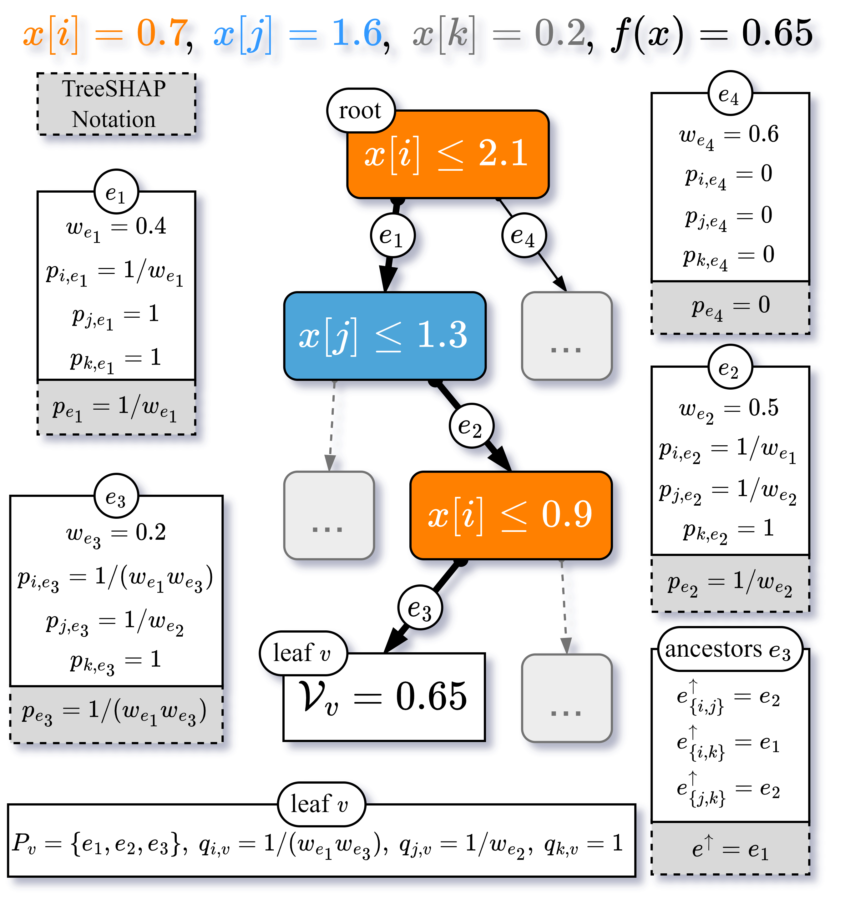
We consider a decision tree as a rooted directed tree with a set of vertices , referred to as decision nodes, and edges . The root node is denoted as . Each decision node consists of a split feature with a threshold value and predictions at the leaf nodes. For each node , we let be the set of edges from the root node to and the set of leaf nodes reachable from , where is the set of all leaf nodes in the tree. For every edge going from to , we denote as the tail of and as the head of , . We consider a weighted tree with weights for every edge , which is defined as the proportion of observed data points at the tail of , that split to the head of . Additionally, we label each edge with the feature associated with the tail of , i.e. the feature that was used to split the observations on the decision node at the source of . Further, and are the edges in and with label . Our notation for decision trees is illustrated in Figure 3.
We also require polynomial arithmetic and refer to the set of polynomials with maximum degree and coefficients in as . Polynomial multiplication is denoted with and division with or . We denote with the inner product of two vectors and refer to the inner product of the coefficients, if polynomials are considered.
Extended Model for Decision Trees.
A decision tree can be decomposed into distinct decision rules for each leaf , which predict , if reaches and zero otherwise. Note that each induces a subspace of at which the prediction of is constant. The decision tree is thus given as . We now define , the prediction rule restricted to a set of active features , where the remaining are considered to be unknown. If the split feature is unknown, we split based on the weights , which is a common practice (Yu et al. 2022). If all features are unknown, we define . When adding feature to the active set, the product of associated weights is replaced by the split criterion. This is formalized as a recursive property , where is the marginal effect of adding to the active set. To define , we let , if satisfies each split criterion regarding features in the path of , i.e. is the region of feature in the induced subspace of by . For the marginal effect of adding feature is then defined as
| (1) |
where is the indicator function. Furthermore, for we define . The restricted rule is thus defined as
| (2) |
For a tree and the restricted model at is then
In the following, we omit the argument in the notation. We proceed to compute the SV of , which is known as path dependent TreeSHAP (Lundberg et al. 2020).
Linear TreeSHAP.
TreeSHAP exploits the tree structure to compute the SV in polynomial time (Lundberg et al. 2020). Linear TreeSHAP improved this computation and provided a theoretical framework by linking the computation to polynomial arithmetic (Yu et al. 2022). Plugging (2) into the definition of the SV and using the fact that , if a feature does not appear in the path, yields
| (3) |
where is the set of all features that appear in . It was shown that this sum can be efficiently stored using the coefficients of a specific polynomial.
For feature , is the coefficient of in , where is the number of features in each path. Note that this corresponds to the non-weighted terms in the sum of (3) for . The SV of a single decision rule can thus be represented as
| (4) |
where is a function that properly weights the coefficients, such that it corresponds to the sum in (3). It is formally defined (Yu et al. 2022) as
| (5) |
We write , where is the degree of . It was then shown that is additive and scale invariant.
Using (4) based on leaf nodes, a representation of the SV in terms of edges is presented, which is explicitly computed by recursively traversing the tree. For this representation, the SP is extended to every edge in the path of as
where the order is such that , i.e. is an operation on the set of polynomials that sums the polynomial while scaling them to the same degree. Note that due to the properties of , we have . For edge and its feature , we further introduce the inter-path value of as
Note that if is the last edge in . An edge-based representation of the SV is then provided.
Theorem 1 (Yu et al. 2022).
Let and denote for the closest ancestor in the set by , where and in case it does not exist. Then,
Using this edge-based representation, Linear TreeSHAP computes the SV by traversing once through the tree. To improve efficiency, the SP is stored in a multipoint interpolation form. For more details, we refer to Appendix B.
3 TreeSHAP-IQ: Computation of Local Shapley Interactions for Tree Ensembles
Computing the exact SV for tree ensembles can reliably quantify the impact of single features on the model’s predictions. However, in many applications, certain features become only meaningful when interacting with other features. In this case, the SV is not sufficient to understand how the model predicts, and more complex explanations in terms of Shapley interactions are necessary. In the following, we propose TreeSHAP Interaction Quantification (TreeSHAP-IQ), an efficient algorithm for computing any-order SII scores, which follows naturally by extending the SP to interactions.
TreeSHAP-IQ can further be applied to the broad class of CIIs (Grabisch and Roubens 1999), which we briefly discuss in Section 3.2. All proofs are deferred to Appendix A.
3.1 Theoretical Foundation of TreeSHAP-IQ
We now present the theoretical foundation of TreeSHAP-IQ. The notations in this section extend on Linear TreeSHAP (Yu et al. 2022) and are illustrated in Figure 3. We compute the S-derivative for and as
| (6) |
which follows from (2) and the recursive property. We thus represent the SII for a single decision rule as follows.
Proposition 2.
For a leaf in , it holds
Proposition 2 yields a compact representation in terms of leaf nodes and decision rules, which reduces to the representation of (4) for single feature subsets. Similar to Linear TreeSHAP, the representation of SII in terms of leaf nodes is not suitable for efficient computation. We thus again establish an edge-based representation, similar to Theorem 1. By Proposition 2, the computation of an interaction for a subset requires knowledge of all with , which have to be tracked during the traversal of the tree. We thus first extend the inter-path values to every feature as
where if satisfies each decision criterion in . Note that and , if is the label of . Our goal in the following is to provide an algorithm similar to Linear TreeSHAP that traverses the decision tree once and recursively computes the interaction scores. The SP thereby remains unchanged, but we introduce further polynomials of order to efficiently maintain the sum as well as the denominator in Proposition 2.
Definition 3 (Interaction Polynomial (IP)).
The IP of and edge is .
Note that the coefficient of in is exactly for . Therefore, the sum of the coefficients of the IP equals the sum in (6). We thus define the coefficient sum.
Definition 4 (Coefficient sum ).
We define the function as . We write , where is the degree of .
Applying to the IP yields the following properties.
Proposition 3.
For the sum of coefficients of the IP, it holds
| (7) |
If there exists with , then .
Proposition 3 shows that corresponds to the edge-based representation of the sum in Proposition 2. If is the last edge in , then for all and thus retrieves the sum in Proposition 2. Furthermore, if , then it is intuitive that all inter-path contributions with are zero, since does not impact the model’s prediction in this part of the tree. This property allows us to update interaction scores only if all features of the subset have occurred in the path. We further describe the quotient in Proposition 2 using another polynomial of order .
Definition 5 (Quotient Polynomial (QP)).
The QP of and edge is .
If is the last edge in of leaf node that contains any feature of , then for every and hence we can rewrite Proposition 2 using Proposition 3 as
| (8) |
Clearly, Proposition 2 reduces to (4) for the case of the SV. In contrast to the SV, the edge-based computation includes all inter-path values of with . To extend Theorem 2, we therefore need to extend the notion of ancestor edges to ancestors with respect to a subset .
Proposition 4.
For a decision rule of a leaf node and a subset , let and as the closest ancestor of in . The SII of is then given by
Using Proposition 4, we can state our main theorem.
Theorem 2.
For , let be the set of edges that split on any feature in , and denote the closest ancestor of in as . The SII is then computed as
Implementation of TreeSHAP-IQ.
Theorem 2 allows for an efficient computation of the SII, with the SP being handled alike to Linear TreeSHAP. The IQ and QP are updated for each interaction subset that contains the feature of . We again use the multipoint interpolation form to store and update the polynomials , and . TreeSHAP-IQ traverses the decision tree once for every explanation point. At each edge (decision node), TreeSHAP-IQ updates all interactions that contain the currently encountered feature, in total. However, the update can be restricted to those interactions, where all features have been observed in the path. We refer to Appendix B for more details.
Complexity of TreeSHAP-IQ
Consider explanation points, as the number of leaves and as the maximum depth of the tree.
Linear TreeSHAP has a computational complexity of and storage complexity of (Yu et al. 2022). We now consider the complexity of TreeSHAP-IQ, if all interactions of order are computed. In contrast to Linear TreeSHAP and the SP, where only the current feature value has to be updated, TreeSHAP-IQ needs to update the IP, the QP and the interaction scores for all interaction subsets that contain the currently observed feature. This increases the computational complexity by a factor of . Furthermore, all interaction scores have to be stored, requiring storage of . To store the IQ and QP, we require further a storage capacity of . The computational complexity is thus summarized as follows. TreeSHAP-IQ complexity for the SII of order Computational Complexity Storage Complexity
For the computation of the SV, the computational complexity of TreeSHAP-IQ is similar to Linear TreeSHAP. The storage capacity is increased by a factor , as we store the IP and QP for every feature. Moreover, for pairwise interactions, TreeSHAP-IQ mirrors the complexity of the computation proposed by Lundberg et al. (2020) using Linear TreeSHAP. However, our method distinguishes itself by relying on a single initialization of the tree parameters.
3.2 Extending TreeSHAP-IQ to General CIIs
TreeSHAP-IQ can be extended to the broad class of CIIs. A CII is defined as with non-negative weights that depend on the interaction order (Grabisch and Roubens 1999; Fumagalli et al. 2023). This includes other approaches of extending the SV to interactions, such as STI and FSI, as well as Banzhaf interactions (Patel, Strobel, and Zick 2021). Observe from the proofs, that different weights in CIIs solely impact the SP, and in particular . To extend the SP for CIIs, we let and scale to the degree of , which does not impact due to the scale invariance. We then observe
where is the CII weight for SII, cf. Definition 1. Recall from (5) that these weights are retrieved from the polynomial . Thus, we generalize to
If is scaled to degree , then is always evaluated with a polynomial of degree . Further, note that for SII, we have , where the quotient is included in the weights, i.e. .
Implementation of CIIs in TreeSHAP-IQ
Using , any CII can be computed by TreeSHAP-IQ. In contrast to , the scale invariance does not hold for CIIs. Therefore, the SP cannot be reduced to the degree . However, if we maintain the SP at the maximum degree , then all previous results apply. If the SP is stored in multipoint interpolation form, then this merely requires a multiplication with the corresponding term of , which can be efficiently precalculated. Thus, the computational complexity is not affected by this extension. Provided , the storage complexity is not affected either.
Datasets # Instances # Features Target Speed-Up Credit Bank Adult Bike COMPAS Titanic California
4 Experiments
We apply TreeSHAP-IQ111All experimental code and the technical appendix can be found at: github.com/mmschlk/TreeSHAP-IQ. on XGBoost (XBG) (Chen and Guestrin 2016), gradient-boosted trees (GBTs), random forest (RF), and decision tree (DT) algorithms on the German Credit (Hofmann 1994), Bank (Moro, Cortez, and Laureano 2011), Adult Census (Kohavi 1996), Bike (Fanaee-T and Gama 2014), COMPAS (Angwin et al. 2016), Titanic (Dawson 1995), and California (Kelley Pace and Barry 1997) datasets, see Table 1. For further experimental results, including a run-time analysis and detailed information on the datasets, models, and pre-processing steps, we refer to Appendix C. We compute additive interactions for single predictions using TreeSHAP-IQ with n-SII of different order.
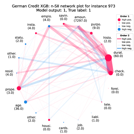
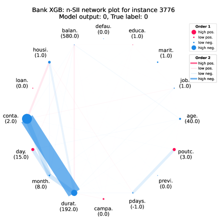
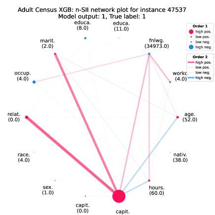
TreeSHAP-IQ Reveals Intricate Feature Interactions.
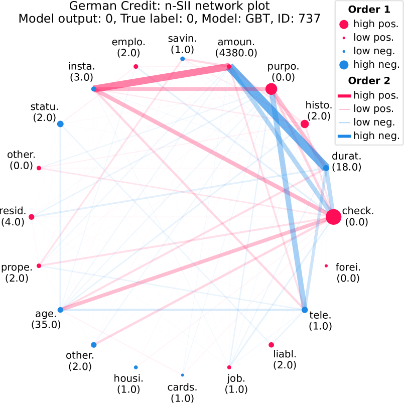
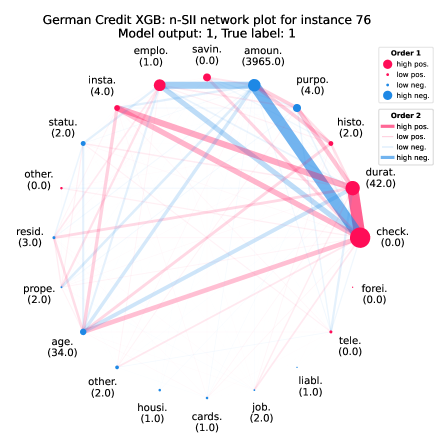
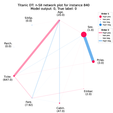
Using TreeSHAP-IQ, we examine the model’s prediction based on higher order interaction effects. We distinguish n-SII scores that positively (red) and negatively (blue) impact the prediction. In Figure 1, we visualize n-SII with . The width of the network vertices (order 1) and the network edges (order 2) describes the absolute value of the corresponding n-SII scores. We observe that there exist features that strongly impact the prediction individually, such as the information about a non-existing checking account. However, the present credit amount strongly impacts the prediction only in interaction with the given installment rate (positively) and duration (negatively).
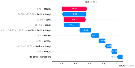
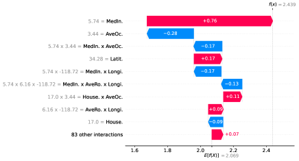
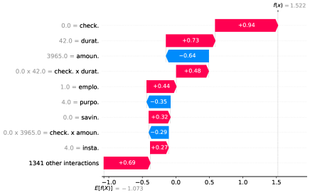
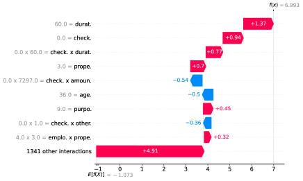
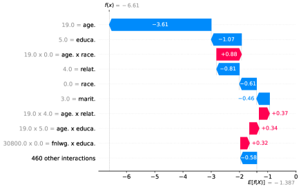
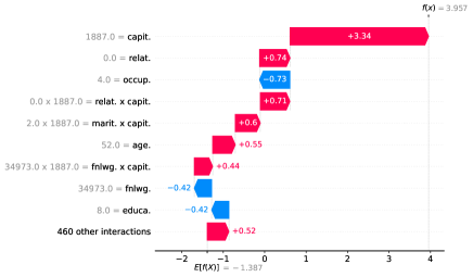
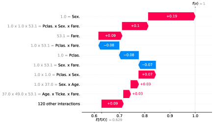
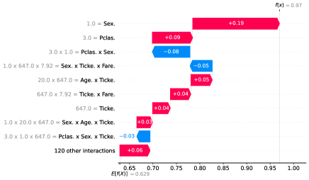
The force plots in Figure 2 illustrate how the additive local explanations change, if higher order interactions are considered. We consider the n-SII scores for for the California housing dataset and an XGBoost regressor. The force plot displays the positive and negative interaction scores starting from the predicted value to the left and right, respectively, sorted by their absolute value. We observe that individual feature effects, such as Longitude, reduce when higher order interactions are considered. The interaction of Longitude and Latitude reveals the importance of the geographic location of this instance.
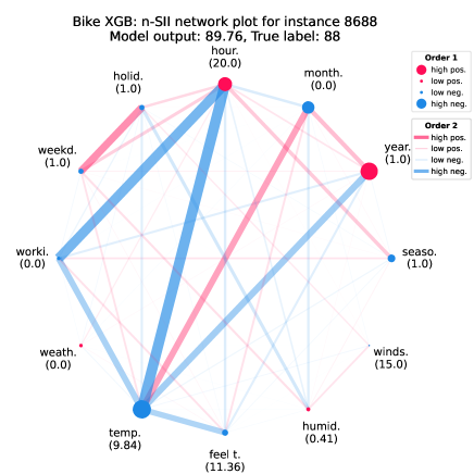
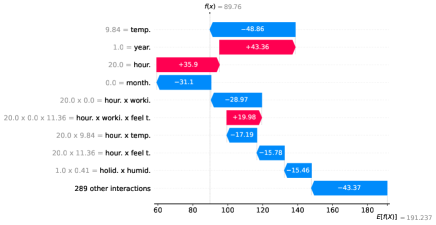
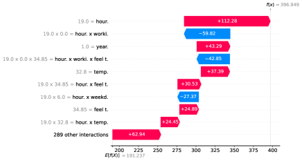
The waterfall chart in Figure 4 displays the explanations of n-SII with order for an instance in the bike dataset. For this instance, it can be seen that the interaction of the evening hour with a non-working day affects the prediction negatively, whereas the interaction with both temperature features contribute positively.
n-SII Plots Quantify Interactions of Each Feature.
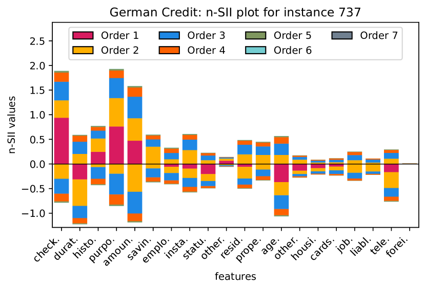
To assess the strength of interaction per individual feature, we utilize the visualization of n-SII values presented by Bordt and von Luxburg (2023). We compute exact n-SII scores up to order for the German Credit dataset. The positive and negative interactions are distributed equally onto each feature in the subset and displayed on the positive and negative axes, respectively. The sum of all stacked bars results in the SV of each feature (Bordt and von Luxburg 2023). In Figure 5, we observe that the interaction effects diminish at order 5, with interactions of orders 6 and 7 being virtually absent. Assuming that interactions decay with higher order, this visualization can be used to find the maximum order to explain the prediction (i.e. from Figure 5).
5 Limitations
TreeSHAP-IQ applies to the broad class of CIIs, provided that its representation in terms of a weighted sum of discrete derivatives is known. For FSI, this representation is only explicitly known for top-order interactions (Tsai, Yeh, and Ravikumar 2023), as FSI is motivated as a solution to a constrained weighted least square problem. Similar to the SV, Shapley interactions strongly rely on how absent features are modeled. In our work, we considered the path dependent feature perturbation (Lundberg et al. 2020), which is linked to the observational approach (Chen et al. 2020). The interventional approach (Lundberg et al. 2020) can be computed with TreeSHAP-IQ, akin to TreeSHAP, but similarly increases the computational complexity by the number of samples used in the background dataset. In this case, more efficient variants should be used instead (Zern, Broelemann, and Kasneci 2023). Both paradigms yield different explanations, where the appropriate choice should be carefully done depending on the application (Chen et al. 2020).
6 Conclusion and Future Work
We presented TreeSHAP-IQ, an efficient method to compute any-order additive Shapley interactions that locally explain single predictions for general ensembles of trees. Akin to SOTA Linear TreeSHAP (Yu et al. 2022), our algorithm is based on a solid theoretical foundation that exploits polynomial arithmetic. We applied TreeSHAP-IQ on SOTA ML models, such as XGBoost (Chen and Guestrin 2016), and several benchmark datasets. We demonstrated that TreeSHAP-IQ reveals intricate feature interactions, which enrich Shapley-based feature attribution.
Utilizing well-known visualization and aggregation techniques from machine learning (Lundberg and Lee 2017; Bordt and von Luxburg 2023) and statistics (Inglis, Parnell, and Hurley 2022) we presented these scores in a manner that is easily understandable and interpretable. While interactions are widely studied in statistics, explaining local predictions using interaction scores, in particular with Shapley-based interactions, is an emerging line of research in the field of XAI. Due to the exponentially increasing number of interactions, we provided intuitive visualizations to present TreeSHAP-IQ scores to practitioners. Nevertheless, it would be beneficial to explore further human-centered post-processing techniques and visualizations, as well as rigorously evaluate the explanatory capabilities of TreeSHAP-IQ with user studies, especially to validate quantitatively that the user’s understanding increases when higher order explanations are presented. Additionally, the n-SII scores define a local generalized additive model (GAM) (Bordt and von Luxburg 2023) that could be further linked to functional decomposition (Hiabu, Meyer, and Wright 2023).
Acknowledgements
We sincerely thank the anonymous reviewers for their work and helpful comments. We gratefully acknowledge funding by the Deutsche Forschungsgemeinschaft (DFG, German Research Foundation): TRR 318/1 2021 – 438445824.
References
- Adadi and Berrada (2018) Adadi, A.; and Berrada, M. 2018. Peeking Inside the Black-Box: A Survey on Explainable Artificial Intelligence (XAI). IEEE Access, 6: 52138–52160.
- Angwin et al. (2016) Angwin, J.; Larson, J.; Mattu, S.; and Kirchner, L. 2016. Machine Bias. There’s software used across the country to predict future criminals. And it’s biased against blacks.
- Bordt and von Luxburg (2023) Bordt, S.; and von Luxburg, U. 2023. From Shapley Values to Generalized Additive Models and back. In International Conference on Artificial Intelligence and Statistics (AISTATS 2023), volume 206 of Proceedings of Machine Learning Research, 709–745. PMLR.
- Boulesteix et al. (2012) Boulesteix, A.-L.; Bender, A.; Lorenzo Bermejo, J.; and Strobl, C. 2012. Random forest Gini importance favours SNPs with large minor allele frequency: impact, sources and recommendations. Briefings in Bioinformatics, 13(3): 292–304.
- Casalicchio, Molnar, and Bischl (2018) Casalicchio, G.; Molnar, C.; and Bischl, B. 2018. Visualizing the Feature Importance for Black Box Models. In Machine Learning and Knowledge Discovery in Databases - European Conference (ECML PKDD 2018), volume 11051 of Lecture Notes in Computer Science, 655–670. Springer.
- Castro et al. (2017) Castro, J.; Gómez, D.; Molina, E.; and Tejada, J. 2017. Improving polynomial estimation of the Shapley value by stratified random sampling with optimum allocation. Computers & Operations Research, 82: 180–188.
- Castro, Gómez, and Tejada (2009) Castro, J.; Gómez, D.; and Tejada, J. 2009. Polynomial calculation of the Shapley value based on sampling. Computers & Operations Research, 36(5): 1726–1730.
- Chen et al. (2023) Chen, H.; Covert, I.; Lundberg, S.; et al. 2023. Algorithms to estimate Shapley value feature attributions. Nature Machine Intelligence, 5: 590–601.
- Chen et al. (2020) Chen, H.; Janizek, J. D.; Lundberg, S. M.; and Lee, S. 2020. True to the Model or True to the Data? arXiv:2006.16234.
- Chen and Guestrin (2016) Chen, T.; and Guestrin, C. 2016. XGBoost: A Scalable Tree Boosting System. In Proceedings of the 22nd ACM SIGKDD International Conference on Knowledge Discovery and Data Mining (SIGKDD 2016), 785–794. ACM.
- Covert and Lee (2021) Covert, I.; and Lee, S. 2021. Improving KernelSHAP: Practical Shapley Value Estimation Using Linear Regression. In The 24th International Conference on Artificial Intelligence and Statistics, (AISTATS 2021), volume 130 of Proceedings of Machine Learning Research, 3457–3465. PMLR.
- Covert, Lundberg, and Lee (2020) Covert, I.; Lundberg, S. M.; and Lee, S. 2020. Understanding Global Feature Contributions With Additive Importance Measures. In Advances in Neural Information Processing Systems 33: Annual Conference on Neural Information Processing Systems 2020 (NeurIPS 2020).
- Dawson (1995) Dawson, R. J. M. 1995. The “Unusual Episode” Data Revisited. Journal of Statistics Education, 3(3).
- Fanaee-T and Gama (2014) Fanaee-T, H.; and Gama, J. 2014. Event Labeling Combining Ensemble Detectors and Background Knowledge. Progress in Artificial Intelligence, 2(2): 113–127.
- Feurer et al. (2020) Feurer, M.; van Rijn, J. N.; Kadra, A.; Gijsbers, P.; Mallik, N.; Ravi, S.; Mueller, A.; Vanschoren, J.; and Hutter, F. 2020. OpenML-Python: an extensible Python API for OpenML. arXiv:1911.02490.
- Friedman (2001) Friedman, J. H. 2001. Greedy function approximation: A gradient boosting machine. The Annals of Statistics, 29(5): 1189–1232.
- Fumagalli et al. (2023) Fumagalli, F.; Muschalik, M.; Kolpaczki, P.; Hüllermeier, E.; and Hammer, B. 2023. SHAP-IQ: Unified Approximation of any-order Shapley Interactions. arXiv:2303.01179.
- Grabisch and Roubens (1999) Grabisch, M.; and Roubens, M. 1999. An axiomatic approach to the concept of interaction among players in cooperative games. International Journal of Game Theory, 28(4): 547–565.
- Harris, Pymar, and Rowat (2022) Harris, C.; Pymar, R.; and Rowat, C. 2022. Joint Shapley values: a measure of joint feature importance. In The Tenth International Conference on Learning Representations, (ICLR 2022). OpenReview.net.
- Herbinger, Bischl, and Casalicchio (2023) Herbinger, J.; Bischl, B.; and Casalicchio, G. 2023. Decomposing Global Feature Effects Based on Feature Interactions. arXiv:2306.00541.
- Hiabu, Meyer, and Wright (2023) Hiabu, M.; Meyer, J. T.; and Wright, M. N. 2023. Unifying local and global model explanations by functional decomposition of low dimensional structures. In International Conference on Artificial Intelligence and Statistics (AISTATS 2023), volume 206 of Proceedings of Machine Learning Research, 7040–7060. PMLR.
- Hofmann (1994) Hofmann, H. 1994. Statlog (German Credit Data). UCI Machine Learning Repository. DOI: 10.24432/C5NC77.
- Hooker (2004) Hooker, G. 2004. Discovering additive structure in black box functions. In Kim, W.; Kohavi, R.; Gehrke, J.; and DuMouchel, W., eds., Proceedings of the Tenth ACM SIGKDD International Conference on Knowledge Discovery and Data Mining (SIGKDD 2004), 575–580. ACM.
- Hooker (2007) Hooker, G. 2007. Generalized Functional ANOVA Diagnostics for High-Dimensional Functions of Dependent Variables. Journal of Computational and Graphical Statistics, 16(3): 709–732.
- Inglis, Parnell, and Hurley (2022) Inglis, A.; Parnell, A.; and Hurley, C. B. 2022. Visualizing Variable Importance and Variable Interaction Effects in Machine Learning Models. Journal of Computational and Graphical Statistics, 31(3): 766–778.
- Jethani et al. (2022) Jethani, N.; Sudarshan, M.; Covert, I. C.; Lee, S.; and Ranganath, R. 2022. FastSHAP: Real-Time Shapley Value Estimation. In The Tenth International Conference on Learning Representations (ICLR 2022). OpenReview.net.
- Ke et al. (2017) Ke, G.; Meng, Q.; Finley, T.; Wang, T.; Chen, W.; Ma, W.; Ye, Q.; and Liu, T. 2017. LightGBM: A Highly Efficient Gradient Boosting Decision Tree. In Advances in Neural Information Processing Systems 30: Annual Conference on Neural Information Processing Systems 2017 (NeurIPS 2017), 3146–3154.
- Kelley Pace and Barry (1997) Kelley Pace, R.; and Barry, R. 1997. Sparse spatial autoregressions. Statistics & Probability Letters, 33(3): 291–297.
- Kohavi (1996) Kohavi, R. 1996. Scaling up the Accuracy of Naive-Bayes Classifiers: A Decision-Tree Hybrid. In Proceedings of International Conference on Knowledge Discovery and Data Mining (KDD 1996), 202–207.
- Kolpaczki et al. (2023) Kolpaczki, P.; Bengs, V.; Muschalik, M.; and Hüllermeier, E. 2023. Approximating the Shapley Value without Marginal Contributions. arXiv:2302.00736.
- Kumar et al. (2021) Kumar, I.; Scheidegger, C.; Venkatasubramanian, S.; and Friedler, S. A. 2021. Shapley Residuals: Quantifying the limits of the Shapley value for explanations. In Advances in Neural Information Processing Systems 34: Annual Conference on Neural Information Processing Systems 2021 NeurIPS 2021, 26598–26608.
- Kumar et al. (2020) Kumar, I. E.; Venkatasubramanian, S.; Scheidegger, C.; and Friedler, S. A. 2020. Problems with Shapley-value-based explanations as feature importance measures. In Proceedings of the 37th International Conference on Machine Learning (ICML 2020), volume 119 of Proceedings of Machine Learning Research, 5491–5500. PMLR.
- Lengerich et al. (2020) Lengerich, B. J.; Tan, S.; Chang, C.; Hooker, G.; and Caruana, R. 2020. Purifying Interaction Effects with the Functional ANOVA: An Efficient Algorithm for Recovering Identifiable Additive Models. In The 23rd International Conference on Artificial Intelligence and Statistics (AISTATS 2020), volume 108 of Proceedings of Machine Learning Research, 2402–2412. PMLR.
- Lundberg et al. (2020) Lundberg, S. M.; Erion, G. G.; Chen, H.; DeGrave, A. J.; Prutkin, J. M.; Nair, B.; Katz, R.; Himmelfarb, J.; Bansal, N.; and Lee, S. 2020. From local explanations to global understanding with explainable AI for trees. Nature Machine Intelligence, 2(1): 56–67.
- Lundberg and Lee (2017) Lundberg, S. M.; and Lee, S. 2017. A Unified Approach to Interpreting Model Predictions. In Advances in Neural Information Processing Systems 30: Annual Conference on Neural Information Processing Systems 2017, NeurIPS 2017, 4765–4774.
- Lunetta et al. (2004) Lunetta, K. L.; Hayward, L. B.; Segal, J.; and Van Eerdewegh, P. 2004. Screening large-scale association study data: exploiting interactions using random forests. BMC Genetics, 5: 32.
- Moro, Cortez, and Laureano (2011) Moro, S.; Cortez, P.; and Laureano, R. 2011. Using Data Mining for Bank Direct Marketing: An Application of the CRISP-DM Methodology. In Proceedings of the European Simulation and Modelling Conference (ESM 2011).
- Patel, Strobel, and Zick (2021) Patel, N.; Strobel, M.; and Zick, Y. 2021. High Dimensional Model Explanations: An Axiomatic Approach. In 2021 ACM Conference on Fairness, Accountability, and Transparency, Virtual Event (FAccT 2021), 401–411. ACM.
- Pedregosa et al. (2011) Pedregosa, F.; Varoquaux, G.; Gramfort, A.; Michel, V.; Thirion, B.; Grisel, O.; Blondel, M.; Prettenhofer, P.; Weiss, R.; Dubourg, V.; VanderPlas, J.; Passos, A.; Cournapeau, D.; Brucher, M.; Perrot, M.; and Duchesnay, E. 2011. Scikit-learn: Machine Learning in Python. Journal of Machine Learning Research, 12: 2825–2830.
- Shapley (1953) Shapley, L. S. 1953. A Value for n-Person Games. In Contributions to the Theory of Games (AM-28), Volume II, 307–318. Princeton University Press.
- Shwartz-Ziv and Armon (2022) Shwartz-Ziv, R.; and Armon, A. 2022. Tabular data: Deep learning is not all you need. Information Fusion, 81: 84–90.
- Slack et al. (2020) Slack, D.; Hilgard, S.; Jia, E.; Singh, S.; and Lakkaraju, H. 2020. Fooling LIME and SHAP: Adversarial Attacks on Post hoc Explanation Methods. In AAAI/ACM Conference on AI, Ethics, and Society (AIES 2020), 180–186. ACM.
- Strumbelj and Kononenko (2014) Strumbelj, E.; and Kononenko, I. 2014. Explaining prediction models and individual predictions with feature contributions. Knowledge and Information Systems, 41(3): 647–665.
- Sundararajan, Dhamdhere, and Agarwal (2020) Sundararajan, M.; Dhamdhere, K.; and Agarwal, A. 2020. The Shapley Taylor Interaction Index. In Proceedings of the 37th International Conference on Machine Learning, (ICML 2020), volume 119 of Proceedings of Machine Learning Research, 9259–9268. PMLR.
- Sundararajan and Najmi (2020) Sundararajan, M.; and Najmi, A. 2020. The Many Shapley Values for Model Explanation. In Proceedings of the 37th International Conference on Machine Learning (ICML 2020), volume 119 of Proceedings of Machine Learning Research, 9269–9278. PMLR.
- Tsai, Yeh, and Ravikumar (2023) Tsai, C.; Yeh, C.; and Ravikumar, P. 2023. Faith-Shap: The Faithful Shapley Interaction Index. Journal of Machine Learning Research, 24(94): 1–42.
- Tsang, Rambhatla, and Liu (2020) Tsang, M.; Rambhatla, S.; and Liu, Y. 2020. How does This Interaction Affect Me? Interpretable Attribution for Feature Interactions. In Advances in Neural Information Processing Systems 31: Annual Conference on Neural Information Processing Systems (NeurIPS 2020), 6147–6159.
- Winham et al. (2012) Winham, S. J.; Colby, C. L.; Freimuth, R. R.; Wang, X.; de Andrade, M.; Huebner, M.; and Biernacka, J. M. 2012. SNP interaction detection with Random Forests in high-dimensional genetic data. BMC Bioinformatics, 13: 164.
- Wright, Ziegler, and König (2016) Wright, M. N.; Ziegler, A.; and König, I. R. 2016. Do little interactions get lost in dark random forests? BMC Bioinform., 17: 145.
- Yang (2021) Yang, J. 2021. Fast TreeSHAP: Accelerating SHAP Value Computation for Trees. arXiv:2109.09847.
- Yu et al. (2022) Yu, P.; Bifet, A.; Read, J.; and Xu, C. 2022. Linear tree shap. In Advances in Neural Information Processing Systems 35: Annual Conference on Neural Information Processing Systems 2022, (NeurIPS 2022).
- Zern, Broelemann, and Kasneci (2023) Zern, A.; Broelemann, K.; and Kasneci, G. 2023. Interventional SHAP Values and Interaction Values for Piecewise Linear Regression Trees. In Thirty-Seventh AAAI Conference on Artificial Intelligence, (AAAI 2023), 11164–11173. AAAI Press.
- Zhang et al. (2021) Zhang, H.; Xie, Y.; Zheng, L.; Zhang, D.; and Zhang, Q. 2021. Interpreting Multivariate Shapley Interactions in DNNs. In Thirty-Fifth AAAI Conference on Artificial Intelligence, (AAAI 2021), 10877–10886. AAAI Press.
Appendix A Proofs
A.1 Proof of Proposition 2
For a leaf in , it holds
Proof.
Let be a decision rule of leaf node . For the S-derivative it follows by the recursive property and (3) that
Plugging this representation into the definition of SII with
yields
This sum is further simplified to
| (9) |
We thus need to show that this term is equal to applied on
With using the scale invariance of the SP, we can scale this polynomial to the degree of , i.e. multiplying it with for every feature not present in , i.e. . This yields with the above that
where the last line follows from the fact that if the feature is not present in the path. As weights the coefficients of this polynomial, we proceed by evaluating the coefficients. When writing the product as a sum, every combination of features appears exactly once, and thus
Hence, it follows for the polynomial of degree that
which is equal to (9) and finishes the proof. ∎
A.2 Proof of Proposition 3
For the sum of coefficients of the IP, it holds
| (10) |
If there exists with , then .
Proof.
We first compute the coefficients of the IP as
Hence,
which finishes the first part of the proof.
Now, let for some . Then,
which finishes the proof. ∎
A.3 Proof of Proposition 4
For a decision rule of a leaf node and a subset , let and as the closest ancestor of in . The SII of is then
Proof.
By Proposition 2, we need to show that the right hand side is equal to
| (11) |
We can simplify the sum on the right hand side, as all terms except the last edge cancel out, to
where we used the scale invariance of and the definition of the QP. For the last edge in the path it holds that for all and thus the argument in is equal to the argument in (11). Furthermore, for the IP, we have by Proposition 3 that
which concludes the proof. ∎
A.4 Proof of Theorem 2
For let be the set of edges that split on any feature in and denote as the closest ancestor of in . The SII is then computed as
Proof.
The model can be represented as a sum of decision rules as and thus by the linearity of SII and Proposition 4
where we added to the scaling factor. Now we have that , i.e. if is a leaf and and edge in its path, then is also reachable from the head of , , and vice versa. We can thus change the summation to
Note that yields a polynomial of degree and the degree of is always equal to . Hence, the polynomials can be summed using the additivity of , which yields
Similarly, for the other term
which finishes the proof. ∎
Appendix B Implementations
In the following, we describe pseudo-code for TreeSHAP-IQ for SII (Section B.1) and general CIIs (Section B.2) and Linear TreeSHAP (Section B.3), as well as its efficient implementation using the multipoint interpolation form for all polynomials.
B.1 TreeSHAP-IQ Algorithm
The pseudo-code for TreeSHAP-IQ is outlined in Algorithm 1.
B.2 Implementation of TreeSHAP-IQ for general CIIs
The pseudo-code of TreeSHAP-IQ applied to an arbitrary CII is outlined in Algorithm 2.
B.3 Implementation of Linear TreeSHAP
The pseudo-code of Linear TreeSHAP is outlined in Algorithm 3.
B.4 Efficient Implementation of Polynomial Operations using Multipoint Interpolation
Linear TreeSHAP and TreeSHAP-IQ rely on multiplication and division for polynomials, as well as evaluating the polynomial coefficients using and . These operations can be efficiently implemented by storing the polynomial in a multipoint interpolation form. Instead of storing the poylnomial, we store its evaluation at base points . Multiplication and division then transfer to vector multiplication and division. The inner product of the coefficients of the polynomial, as required for and , can be efficiently computed using the following lemma.
Lemma 1 (Yu et al., 2022).
Let with coefficients , respectively. Then , where corresponds to the Vandermonde matrix with entries .
As proposed by Yu et al. (2022), we use the Chebyshev points to evaluate the polynomial, as they are optimal in terms of numerical stability. Using the Chebyshev points , the values have to be precomputed, where refers to the coefficients of . It is thus required to precompute as many values as the degree of the given polynomial.
Appendix C Experiments
This section contains further information on the experiments and additional results like a run-time analysis in Section C.2
C.1 Dataset and Model Descriptions
This section contains detailed information about the datasets, the required pre-processing steps and the model fitting.
Models
The following tree-based models are used in our experiments.
-
•
XGBoost (XBG) (Chen and Guestrin 2016)
XGBoost is an ensemble learning algorithm based on gradient boosting. It utilizes decision trees as base learners and optimizes a user-defined loss function through an iterative process. XGBoost incorporates regularization techniques to control model complexity and improve generalization. In our experiments, we relied on the XGBoost library222https://xgboost.readthedocs.io/en/stable/. -
•
Gradient-Boosted Tree (GBT)
Gradient-Boosted Trees are an ensemble learning method that combines multiple weak learners, here decision trees, in a sequential manner. It trains each tree to correct the errors made by the previous ones, effectively reducing the overall prediction error. We used the default parametrization of the GradientBoostingClassifier and GradientBoostingRegressor classes from the scikit-learn library (Pedregosa et al. 2011) -
•
Random Forest (RF)
Random Forest is an ensemble learning algorithm that constructs a collection of decision trees by using bootstrapped subsets of the training data and random feature selection. The predictions from individual trees are then aggregated to make a final prediction. This technique reduces overfitting and enhances model robustness compared with single decision trees. We used the default parametrization of the RandomForestClassifier and RandomForestRegressor classes for classification and regression tasks, respectively (Pedregosa et al. 2011). -
•
Decision Tree (DT)
A Decision Trees is a simple yet powerful model that makes predictions by recursively splitting the data based on the most informative features. Each internal node represents a decision based on a feature, and each leaf node represents a prediction. Decision Trees are prone to overfitting, but they serve as the fundamental building blocks for ensemble methods like Random Forest and Gradient-Boosted Trees. We used the default parameterization of the DecisionTreeClassifier and DecisionTreeRegressor classes in the scikit-learn library (Pedregosa et al. 2011).
Datasets
The following dataset are used in our experiments. The data was either directly retrieved from the cited sources or via scikit-learn (Pedregosa et al. 2011) or openml (Feurer et al. 2020).
-
•
German Credit (Hofmann 1994)
The German Credit dataset consists of credit applicants’ information from a German bank, including 20 attributes such as age, employment status, credit history, and risk assessment outcomes. It contains 1,000 instances, and the primary prediction task involves classification to determine whether an applicant is a “good” or “bad” credit risk based on their attributes. The dataset was retrieved from the UCI repository333http://archive.ics.uci.edu/dataset/144/statlog+german+credit+data. -
•
Bank (Moro, Cortez, and Laureano 2011)
The Bank dataset originates from a Portuguese banking institution and includes customer-related attributes, marketing campaign details, and the outcome of customers subscribing to term deposits. It contains 45,211 instances, and the primary prediction task is classification, aiming to predict whether a customer will subscribe to a term deposit or not. We retrieved the dataset via openml and the identifier 1461. -
•
Adult Census (Kohavi 1996)
Also known as the “Census Income” or “Adult Income” dataset, it contains socio-demographic attributes of individuals along with their income levels. It contains 45,222 instances and 14 attributes, and the main prediction task is classification, aiming to predict whether an individual’s income exceeds per year. We retrieved the dataset via openml and the identifier 1590. -
•
Bike (Fanaee-T and Gama 2014)
This dataset involves information from a bike-sharing program, encompassing attributes like weather conditions, time, and bike rental counts. It contains 17,379 instances and 12 attributes, and the primary prediction task is regression, aiming to predict the count of bike rentals (a continuous value) based on the provided attributes. We retrieved the dataset via openml and the identifier 42712. -
•
COMPAS (Angwin et al. 2016)
The COMPAS dataset comprises criminal defendant attributes and recidivism predictions generated by a proprietary software tool. It contains instances and attributes, and the main prediction task is classification, aiming to predict whether a criminal defendant is likely to recidivate or not. We retrieved the “simplified” dataset from Kaggle444https://www.kaggle.com/datasets/danofer/compass, which was presented in a blog post555https://blog.fastforwardlabs.com/2017/03/09/fairml-auditing-black-box-predictive-models.html. -
•
Titanic (Dawson 1995)
The Titanic dataset records passenger information from the ill-fated Titanic voyage, including features like age, gender, class, and survival status. It contains 891 instances and 9 attributes, and the core prediction task is classification, aiming to predict whether a passenger survived the Titanic disaster or not. The data was retrieved from Kaggle666https://www.kaggle.com/c/titanic/data. -
•
California (Kelley Pace and Barry 1997)
The California housing dataset encompasses housing-related attributes for various geographical regions in California. It contains 20,640 instances and 8 attributes, and the primary prediction task is regression, aiming to predict the median value of owner-occupied homes in California based on the provided attributes. The dataset was retrieved from scikit-learn.
Pre-processing and Model Training
The following list contains all pre-processing steps for each dataset to reproduce the experiments. For further details we refer to the technical supplement containing all experiment scripts and these steps. We base most of the data transformation on scikit-learn (Pedregosa et al. 2011). All models were trained with a 70%, 30% training split and fixed random seeds.
-
•
German Credit: We transform the categorical columns (“checkingstatus”, “history”, “purpose”, “savings”, “employ”, “status”, “others”, “property”, “otherplans”, “housing”, “job”, “tele”, and “foreign”) into integer values via an ordinal encoding. We binarize the label into and .
-
•
Bank: We transform the categorical columns (“job”, “marital”, “education”, “default”, “housing”, “loan”, “contact”, “day”, “month”, “campaign”, and “poutcome”) into integer values via an ordinal encoding. We binarize the label into and . Lastly, we drop rows containing null values.
-
•
Adult Census: We drop rows containing null values and transform the categorical columns (“workclass”, “education”, “marital-status”, “occupation”, “relationship”, “race”, “sex”, “native-country”, and “education-num”) into integer values.
-
•
Bike: We transform the categorical columns (“season”, “year”, “month”, “holiday”, “weekday”, “workingday”, and “weather”) into integer values via an ordinal encoding and drop rows containing null values.
-
•
COMPAS: The dataset was used as-is and no data transformation was applied.
-
•
Titanic: We transform the categorical columns (“Sex”, “Ticket”, “Cabin”, and “Embarked”) into integer values via an ordinal encoding. We impute missing values in categorical and numerical features with the mode and median values respectively.
-
•
California: The dataset was used as-is and no data transformation was applied.
| Datasets | # Instances | # Features | Target | Performance ( or Accuracy) | |||
|---|---|---|---|---|---|---|---|
| XGB | GBT | RF | DT | ||||
| German Credit | 0.7542 | 0.7700 | 0.7533 | 0.6833 | |||
| Bank | 0.9064 | 0.9031 | 0.9020 | 0.8941 | |||
| Adult Census | 0.8715 | 0.8655 | 0.8568 | 0.8524 | |||
| Bike | 0.9464 | 0.8442 | 0.8840 | 0.8796 | |||
| COMPAS | 0.6695 | 0.6776 | 0.6646 | 0.6609 | |||
| Titanic | 0.7761 | 0.8059 | 0.7947 | 0.7723 | |||
| California | 0.8315 | 0.8317 | 0.7723 | 0.5945 | |||
C.2 Run-time Analysis
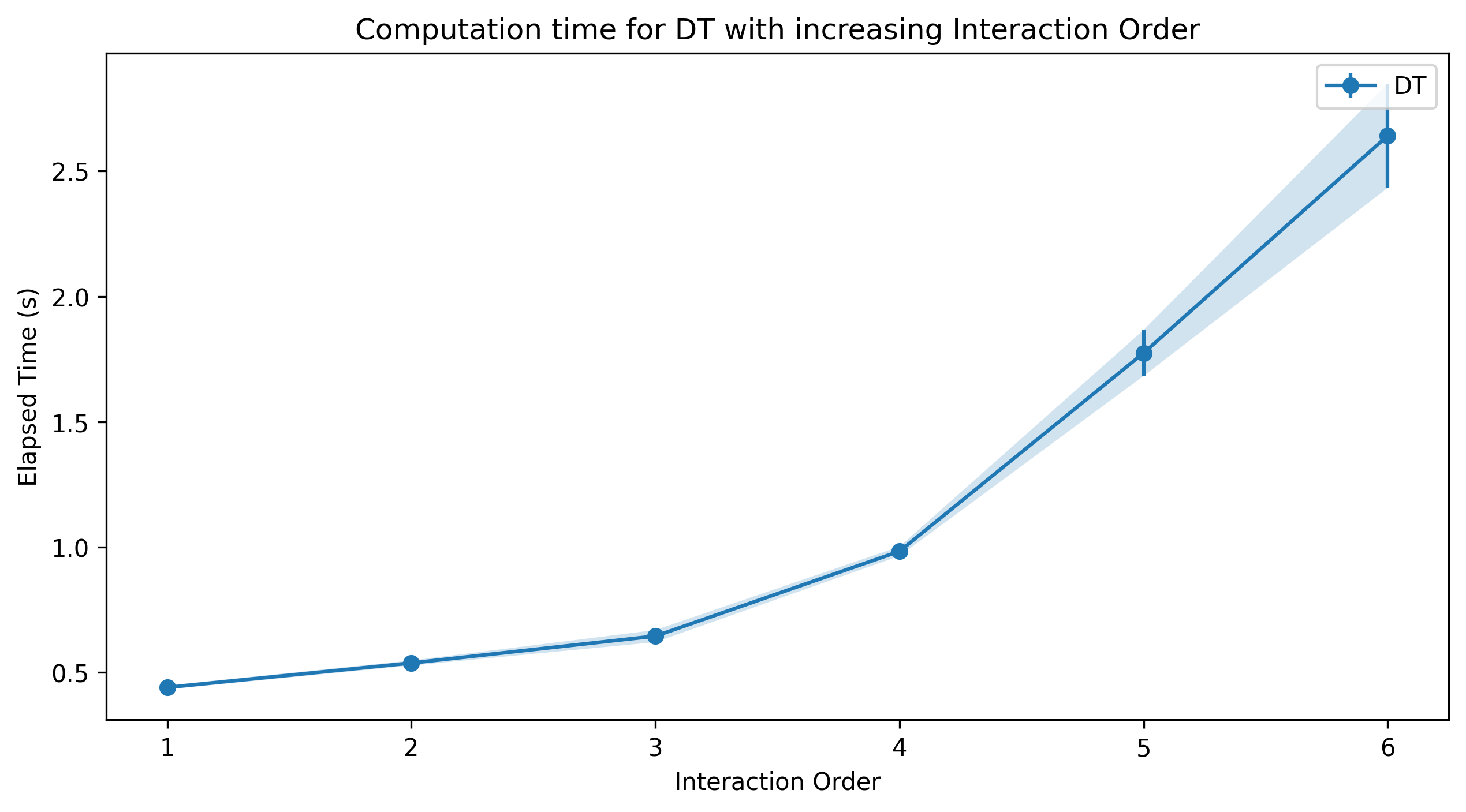
In this section, we provide a run-time analysis that validates our theoretical finding about the runtime complexity of our algorithm. As described in Section 3.1, the run-time complexity of TreeSHAP-IQ for all interactions of order is , where corresponds to the number of explanation points, corresponds to the maximum depth of the tree and is the number of leaves in the tree. Clearly, there are three components that affect the run-time. First, the number of explanation points scales linearly, which is clear and will not be further considered. We thus will keep in the following. Second, the tree complexity, given by both, the number of leaves and depth of the tree affect the complexity jointly. Note, that these values are highly dependent on each other. Third, the order of interactions affects the complexity in an exponential manner, given by the binomial coefficient. In the following, to account for irregularities in the processing times, we run every explanation times and average over the run-times and show the corresponding standard deviations.
Naive Comparison
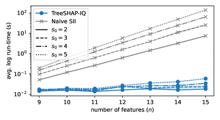
We compare TreeSHAP-IQ’s run-time for computing SII values up to order with a naive computation of SII. For this comparison, we create a separate synthetic classification dataset of samples and number of features for all (we use the make_classification function from sklearn). We fix the tree-depth to and fit a decision tree for each dataset. We make sure that the trees all consists of approximately the same number of nodes (i.e. all trees reach the maximum depth). We then compute the SII values up to order with TreeSHAP-IQ and through a naive brute force computation over all combinations of subsets. We plot the log run-time of TreeSHAP-IQ and the naive SII computation in Figure 6. The comparison shows that the naive calculation scales exponentially with the number of features, while TreeSHAP-IQ scales polynomially for each interaction order .
Run-time by Tree Complexity
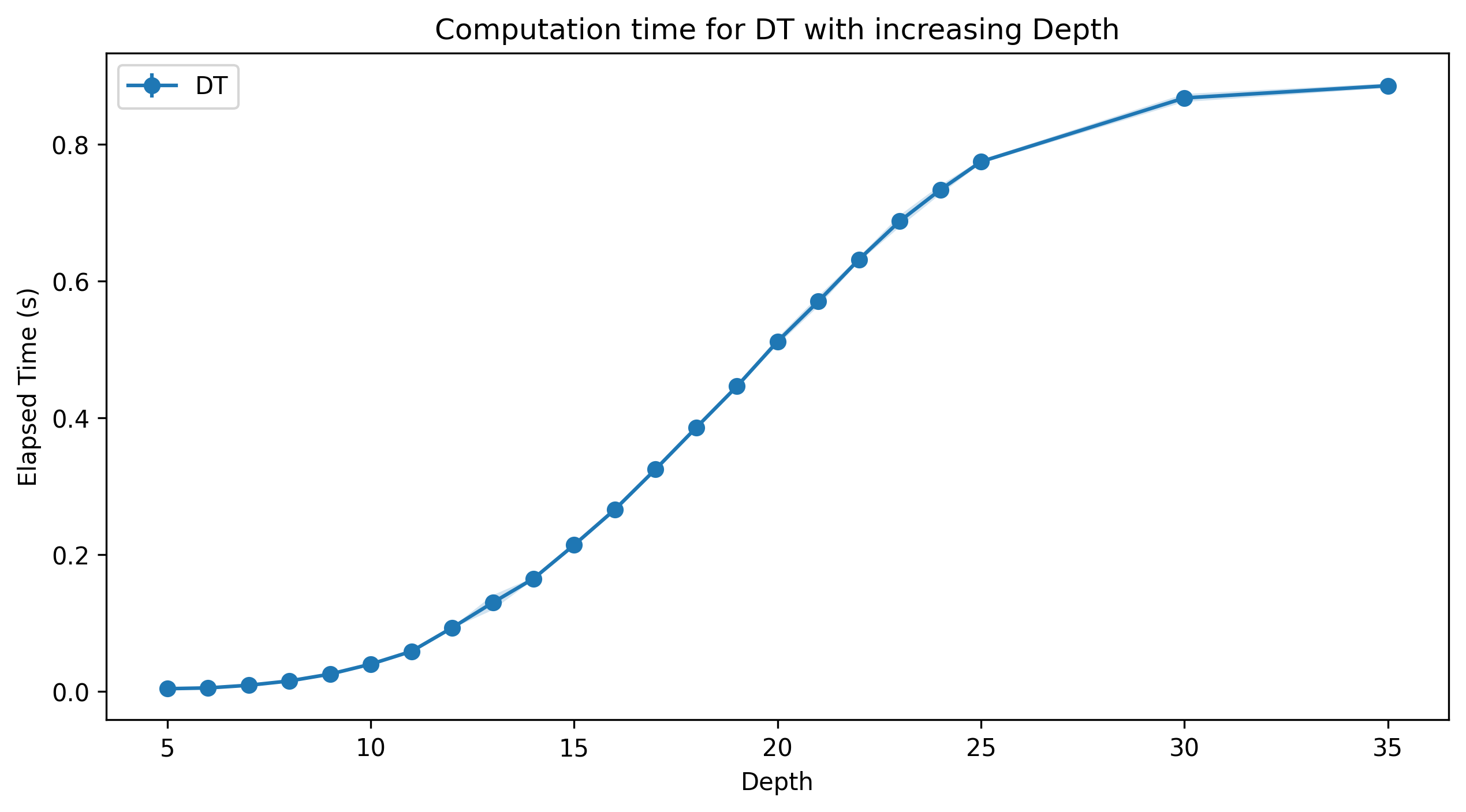
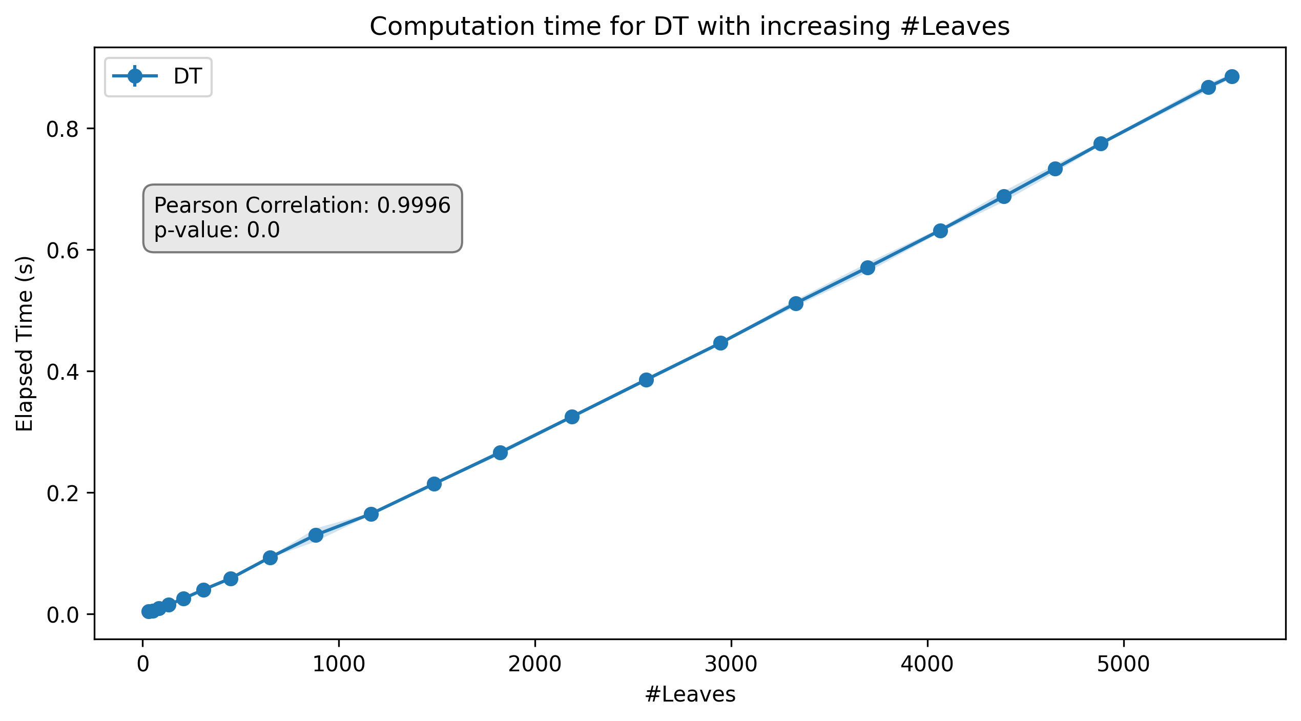
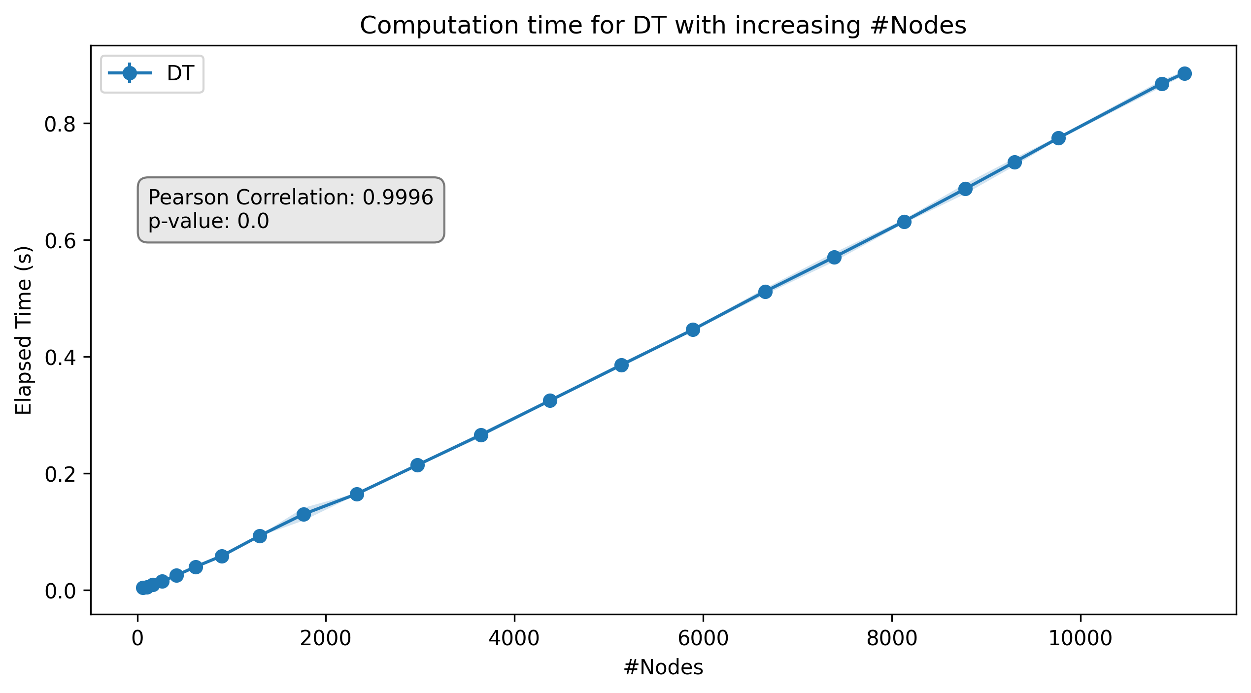
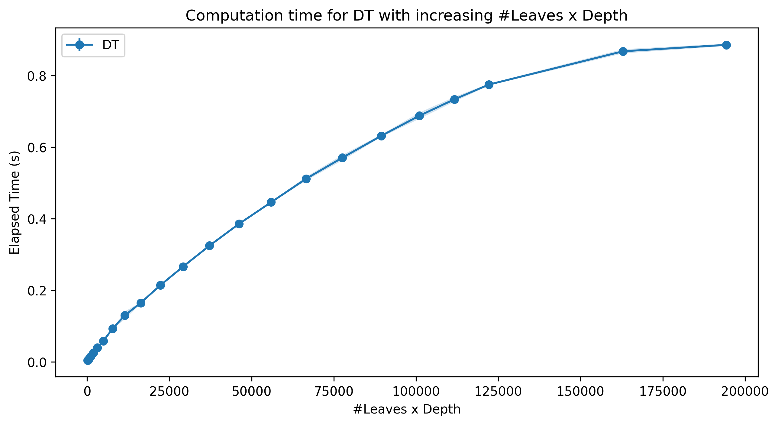
We now illustrate the run-time by the tree complexity, where we compute always pairwise interactions (). The results are shown in Figure 7. We observe a linear relationship of the run-time and the number of vertices, as well as the number of leaves. The run-time compared with the maximum depth of the tree admits a sub-linear behavior at higher depths. This can be explained by the increasing number of paths in the DT that are shorter than the maximum depth, which increasingly occurs at higher depths. Lastly, we also observe this sub-linear behavior in terms of the number of leaves times the depth, which again is explained by the overestimation of operations.
Run-Time by Number of Interactions
We illustrate the run-time depending on the number of interactions for a fixed DT of depth . The results are shown in Figure 8. Note that interactions are only updated, if all features have appeared in the observed path. This is results in far less evaluations, especially for higher order interactions. Again, this is a consequence of the structure of the DT, where only very few paths admit the maximum depth.
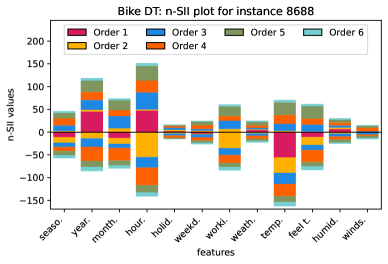
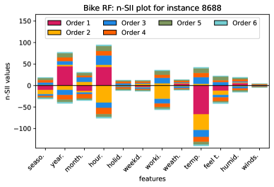
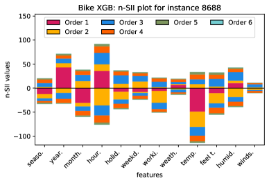
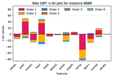
C.3 Additional n-SII Plots
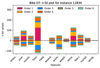
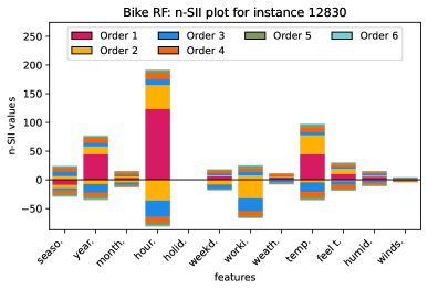
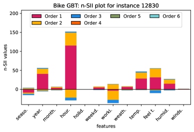
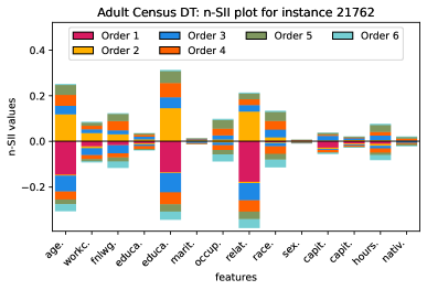
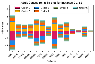
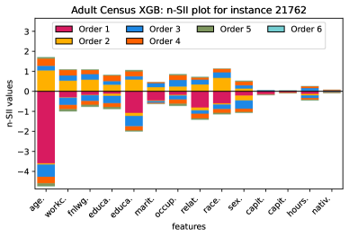
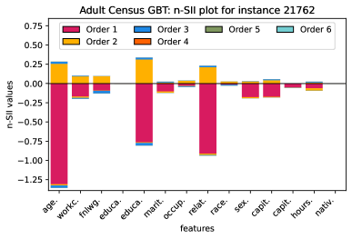
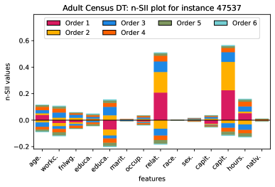
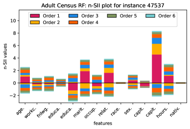
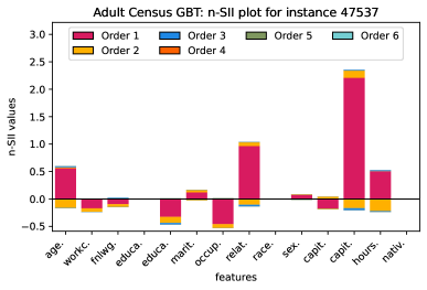
In this section, we compare the strength and nature of interactions present in different model architectures. We generate the n-SII plots of order for the predictions of two randomly selected instances in the Bike and Adult Census dataset. The results for the bike dataset are shown in Figure 9 and Figure 10. The results for the Adult Census dataset are shown in Figure 11 and Figure 12.
We observe that the levels of interaction effects differ significantly among different predictions and different model architectures. For the Bike dataset, the prediction in Figure 10 has higher interaction effects than the prediction in Figure 9. Further, it can be seen that the well-performing XGB model exhibits a high amount of interaction, whereas the relatively poor-performing GBT has little interactions present. Furthermore, as expected the DT exhibits a high level of interaction effects among both predictions, as this method is not an esemble of weak learning algorithms, which are expected to have less interaction effects.
In the Adult Census dataset, we observe a similar pattern for XBG and GBT. Notably, for these instances, XGB exhibits less interaction effects than RF, although the overall performance of XGB is superior. Again, we observe a high amoung of higher order interactions present in the DT. However, its performance is worse than for all ensemble methods. Notably, the RF and the DT exhibit more similar interaction effects than the other models. This could be seen as an indication that the learned functional relationship in gradient boosting approaches differs from classical DT learning schemes. However, observing two local interaction effects does not allow to conclude this rigorously, which would require a global study of interaction effects in the corresponding models.


C.4 Further Experimental Results on Benchmark Datasets
German Credit Dataset
We display n-SII interaction effects up to order in a network plot and effects up to order in a waterfall chart for two randomly selected instances of the German Credit dataset predicted with a XGB. The results are shown in Figure 13.
Bank Dataset
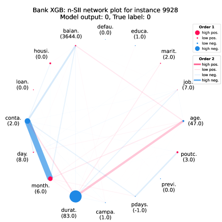
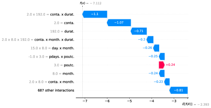
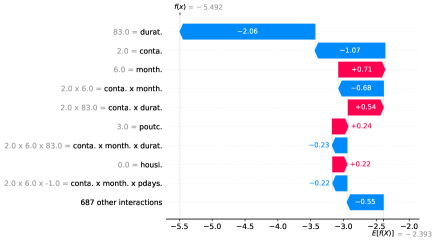
We display n-SII interaction effects up to order in a network plot and effects up to order in a waterfall chart for two randomly selected instances of the Bank dataset predicted with XGB. The results are shown in Figure 14.
Adult Census Dataset
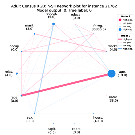
We display n-SII interaction effects up to order in a network plot and effects up to order in a waterfall chart for two randomly selected instances of the Adult Census dataset predicted with XGB. The results are shown in Figure 15.
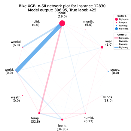
Bike Dataset
We display n-SII interaction effects up to order in a network plot and effects up to order in a waterfall chart for two randomly selected instances of the Bike dataset predicted with XGB. The results are shown in Figure 16.
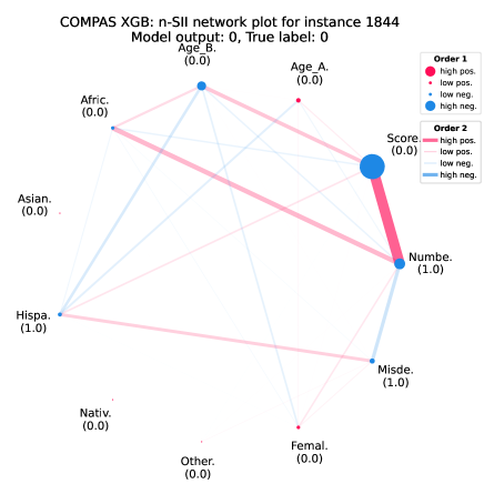
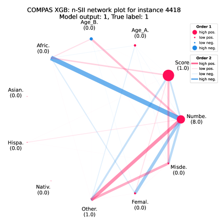
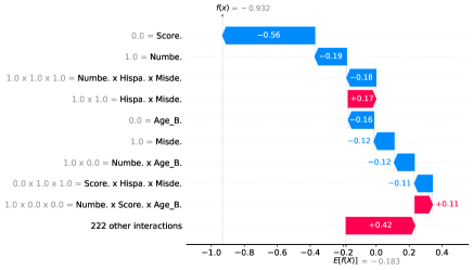
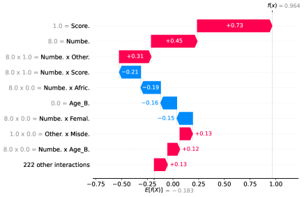
COMPAS Dataset
We display n-SII interaction effects up to order in a network plot and effects up to order in a waterfall chart for two randomly selected instances of the COMPAS dataset predicted with a GBT. The results are shown in Figure 17.
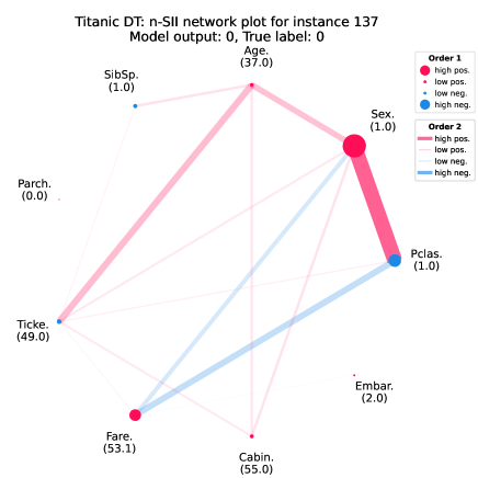
Titanic Dataset
We display n-SII interaction effects up to order in a network plot and effects up to order in a waterfall chart for two randomly selected instances of the Titanic dataset predicted with a DT. The results are shown in Figure 18.
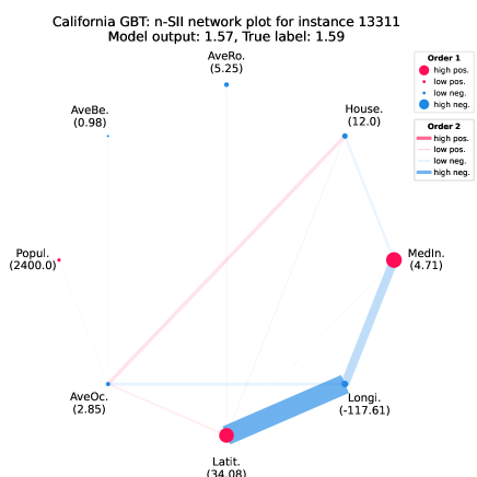
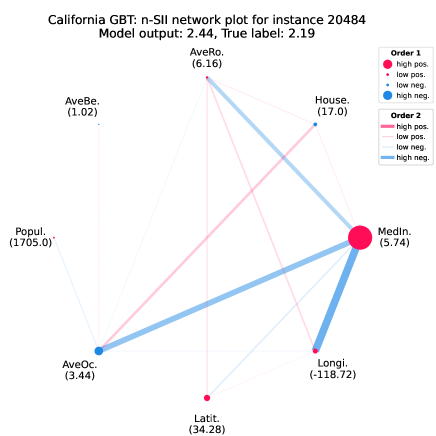
California
We display n-SII interaction effects up to order in a network plot and effects up to order in a waterfall chart for two randomly selected instances of the California dataset predicted with a GBT. The results are shown in Figure 19.