Resource-constrained stereo singing voice cancellation

Abstract

We study the problem of stereo singing voice cancellation, a subtask of music source separation, whose goal is to estimate an instrumental background from a stereo mix. We explore how to achieve performance similar to large state-of-the-art source separation networks starting from a small, efficient model for real-time speech separation. Such a model is useful when memory and compute are limited and singing voice processing has to run with limited look-ahead. In practice, this is realised by adapting an existing mono model to handle stereo input. Improvements in quality are obtained by tuning model parameters and expanding the training set. Moreover, we highlight the benefits a stereo model brings by introducing a new metric which detects attenuation inconsistencies between channels. Our approach is evaluated using objective offline metrics and a large-scale MUSHRA trial, confirming the effectiveness of our techniques in stringent listening tests.

Index Terms—  singing voice cancellation, music source separation

1 Introduction

In this work we present a study of optimisation and evaluation of a Singing Voice Cancellation (SVC) system. We analyse the performance of such as system in limited computational resource scenarios and understand which factors most affect output quality. SVC consists of removing the singing voice from the instrumental background in a fully mixed song, and can be interpreted as a special case of Music Source Separation (MSS). The main difference lies in the fact that MSS aims to retrieve one separate stem for each source present in the mix, while SVC considers only instrumental accompaniment as desired source.

Recent advances in deep learning have led to significant performance improvements in both SVC and MSS, leading to much improved objective metrics. MSS algorithms typically use a spectral [1] or waveform [2] representation. In the first case, both input and output are expressed in the time-frequency domain and popular solutions adopt a U-Net architecture [1, 3], combined with band-split RNN [4], conditioning mechanism [5] or multi-dilated convolutions [6]. Inspired by Wave-Net [7], waveform-based MSS methods tackle the problem end-to-end. An example is Demucs [2], which uses 1-D convolutional encoder and decoders with a bidirectional LSTM. Later versions of Demucs include a spectral branch [8] and transformer layers [9]. Similar approaches have been adopted for Singing Voice Separation [10, 11]. All of these methods produce high quality results but are often designed to be run offline and in a non-causal setup, i.e., having access to the complete audio input, and no constraints on memory or run-time. These methods are not suitable for challenging yet realistic scenarios, where separation happens on low-memory edge devices, under streaming conditions and with hard constraints on processing time. Efficient solutions have been proposed to tackle speech source separation under these circumstances. Conv-TasNet [12] is an end-to-end masking-based architecture which employs 1-D convolutional encoder and decoder, a Temporal Convolutional Network (TCN)-based separator and depth-wise convolutions to reduce network size. This architecture has also been adapted and expanded to address MSS [13, 14].

In this work Conv-TasNet is adapted and optimised for SVC such that the output is of comparable quality to more resource-hungry networks. Such architecture guarantees a low-memory footprint thanks to a limited number of parameters, and is able to operate in real-time. We train the model on a large dataset, to achieve high quality output and we show how training dataset size and quality affect the model’s output quality. The main contributions in this work are:

• To match a real-world setup, we modify Conv-TasNet to take advantage of stereo input and to produce stereo output. This design improves vocal attenuation consistency across stereo channels, and we propose a new stereo metric to verify this improvement.

• We propose a stereo separation asymmetry metric able to measure stereo artifacts and show that the proposed stereo architecture helps to prevent them.

• To validate the proposed approach, we conduct experiments to evaluate objectively and subjectively using a MUSHRA-style test.

We show that a relatively small and specialised model with appropriate training can reach outstanding high quality comparable to much larger models.

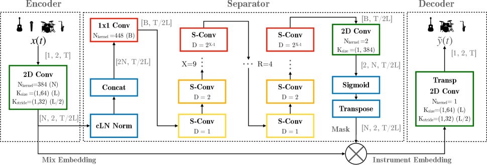
(a) Network Architecture

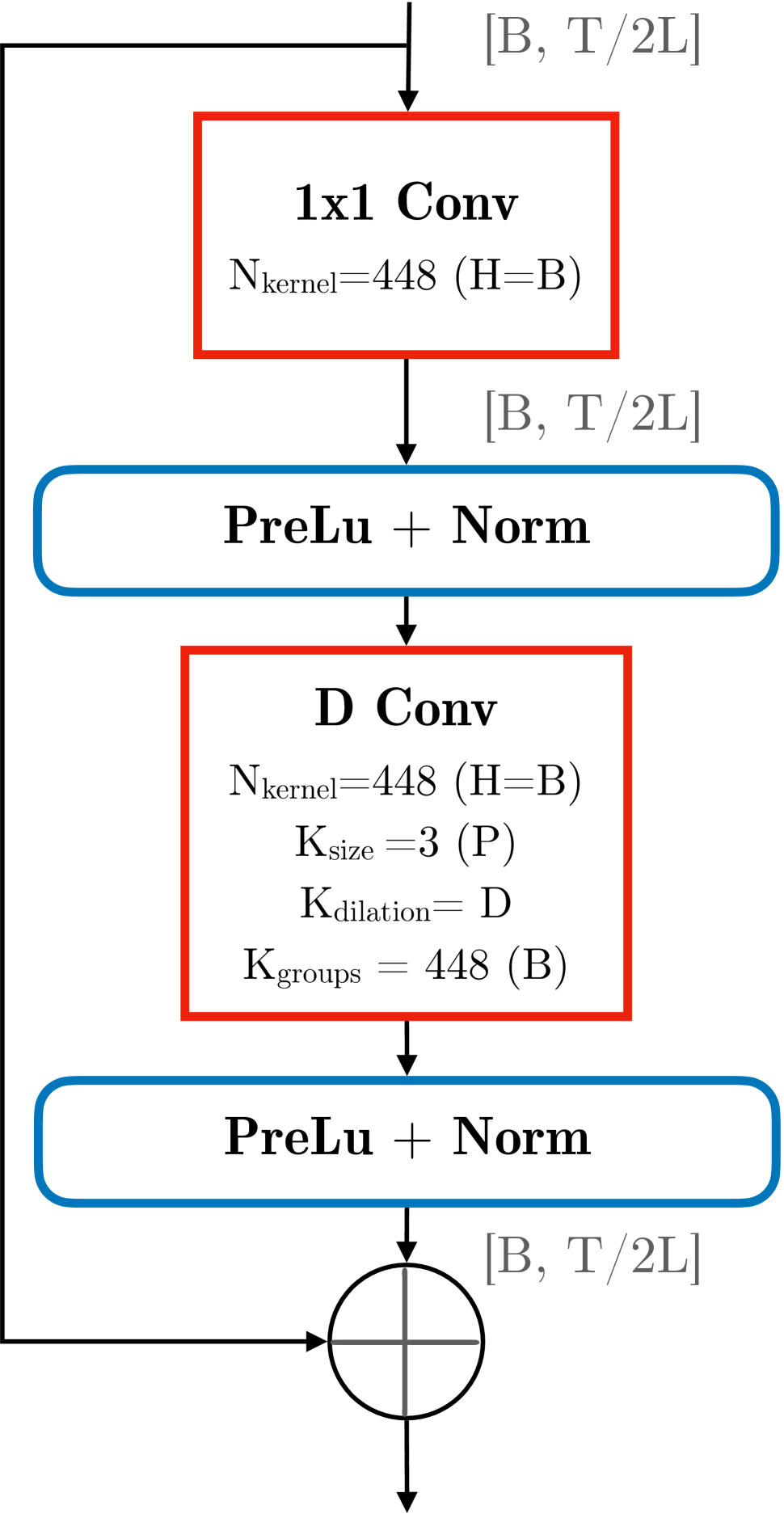
(b) S-Conv Block

Fig. 1: Vox-TasNet architecture and S-Conv block in detail. Letters in parenthesis follow the original notation used in [12]. In square brackets we report input dimensionality as [Ch, W, H] throughout the network.

2 Method

A sampled stereo audio signal $x(t)\in\mathbb{R}^{2}$ with $t\in[0,T)$, which corresponds to a fully mixed track, can be modelled as a linear sum of an instrumental or accompaniment stem $y(t)$ and a vocal stem $v(t)$, i.e., The goal of our system is to estimate $y(t)$ in real-time and with low memory requirements. A real-time scenario implies that the network output should be produced with low-latency. This forces the model to be almost causal, i.e., the output in a specific time instant depends largely on past input samples and possibly a small portion of future samples, i.e., look-ahead, which can be buffered. To be able to satisfy low memory footprint requirements, it is necessary to limit the number of network parameters.

2.1 Network Architecture

We propose Vox-TasNet, an adaptation of Conv-TasNet [12] to the task of SVC in a stereo setup, hence able to jointly estimate both left and right channels. Similar to Conv-TasNet, the network follows a masking-based approach and is composed of three modules, as shown in Fig. 1. The Encoder block reduces time resolution of the raw audio waveform using a two-dimensional convolutional (2D Conv) layer. This creates separate embeddings for the left and right channels of the mix whilst benefiting from the information in both. These embeddings are stacked and fed into the Separator block. The Separator block consists of multiple stacks of separable-depthwise convolutional (S-Conv) layers with increasing dilation and estimates masks for the left and right channel representations. Only the S-Conv layers in the first group are non-causal, making the Separator block almost entirely causal. This allows the network to look ahead for a small time interval. Masking is applied via element-wise multiplication and the resulting masked representations are fed into the Decoder (Transp 2D Conv), which outputs stereo audio accompaniment. Aside from the stereo setup, there are two main differences between Vox-TasNet and Conv-TasNet. First, the Separator’s skip connections are removed to reduce memory footprint, as originally proposed in [15]. Second, we increase the number of S-Conv layers in each group but dimensionality is fixed inside each S-Conv layer, rather than expanded and squeezed. This choice allows the separator to learn longer time dependencies, without increasing the number of parameters.

2.2 Stereo separation asymmetry metric

During informal listening experiments, we noticed that single-channel model produced SVC results which were audibly inconsistent across channels in terms of loudness and attenuation. On the other side, a stereo-native architecture is able to prevent these artifacts and exploit cross-channel information as well. This lead us to devise a stereo separation asymmetry metric which attempted to measure this effect.

Let’s consider a source separation metric, i.e., SI-SDR. It can be formulated in a frame-wise setup, i.e., comparing short frames of prediction and ground-truth signal. Let us define $(\text{SI-SDR}_{L}(n)$, $\text{SI-SDR}_{R}(n))$ as the frame-wise metric computed for $N$ windows of length $W$ and hop size $H$ on left channel and right channel respectively, with $n$ corresponding to window index. We define $\Delta_{\text{SI-SDR}}(n)=|\text{SI-SDR}_{L}(n)-\text{SI-SDR}_{R}(n)|$ as the absolute value of difference between left and right frame-wise metric values. We use as stereo metric $\text{SSA}_{\text{SI-SDR}}=\frac{1}{N}\sum_{n}\Delta_{\text{SI-SDR}}(n)$, as the average over time of $\Delta_{\text{SI-SDR}}(n)$ . Larger values of $\text{SSA}_{\text{M}}$ corresponds to large difference between left and right channel’s separation metric distance over time, hence quality inconsistency. Note that $\Delta_{\text{SI-SDR}}(n)$ and $\text{SSA}_{\text{SI-SDR}}$ can be defined for any other dB-based source-separation metric (i.e., SIR or BSS-Eval metrics).

3 Experimental Setup

To train and validate our system, we consider four different datasets. Three datasets are internal and we will refer to them with $\mathcal{A}$, $\mathcal{B}$ and $\mathcal{C}$. For benchmarking against state-of-the-art models, we use the publicly available MUSDB [16] dataset. In order to be compatible with the task of SVC, the instrumental accompaniment track is obtained by linearly summing the bass, drums and other stems. Dataset specifications are reported in Table 1. For all internal datasets, we apply a pre-processing step to filter out tracks for which the vocal stem is silent for more than 50% of the song. Note from Table 1 that $\mathcal{C}$ is larger than $\mathcal{A}$ and $\mathcal{B}$, but not musically curated by experts hence potentially contains noisier samples.

Dataset	Num Tracks (Train/Test)	Curated	Use
$\mathcal{A}$	3,290	Yes	Train
$\mathcal{B}$	3,797 (3,375/422)	Yes	Train/Test
$\mathcal{C}$	13,625	No	Train
MUSDB	150 (100/50)	Yes	Train/Test

Table 1: Datasets specifications

To have comparable experiments, we use a fixed set of training parameters in all of our experiments. Sampling rate is fixed at $44,100$ Hz, and each training sample is composed of $4$ s of stereo audio, randomly sampled from each song at training time. The batch size is equal to 6 and each model is trained for 500 epochs. We use the Adam optimizer [17] with an initial learning rate 0.0001, scheduled with decay parameter equal to 0.99. The loss function is a weighted average of L1 distance in time domain and multi-resolution spectral L1 distance using window lengths equal to $0.01$ s, $0.02$ s and $0.09$ s and hop-size equal to half of window lengths. Time and spectral losses are weighted with weights $0.875$ and $0.125$ respectively.

As a strong baseline, we use HybridDemucs [8], a large music source separation model without real-time or memory constraints. We aim to match the quality obtained with HybridDemucs, while keeping as reference a resource-constrained scenario. HybridDemucs is trained on the augmented MUSDB dataset and extracts four separate stems from the original mix: drums, bass, vocal and others. We obtain the accompaniment mix as the sum of drums, bass and others stems. Additionally, we consider a mono version of Vox-TasNet, namely MonoVox-TasNet. It has a similar architecture to Vox-TasNet, as shown in Fig 1, but 2-D convolutions are replaced with 1-D convolutions. A stereo output is obtained by separately processing left and right channel and concatenating the results.

To evaluate the proposed system, we take advantage of both objective and subjective evaluation. For objective evaluation, we use Scale Invariant Source-to-Distortion Ratio (SI-SDR) [18] computed between the ground-truth accompaniment and the estimated accompaniment. Moreover, we use the separation symmetry metric presented in Section 2.2, computed using SI-SDR with $W=1.5$ s and $H=0.75$ s, to evaluate out stereo vs mono model. As objective metrics do not always correlate strongly with human perception of audio quality [19], we report subjective evaluation results obtained via a Multiple Stimuli with Hidden Reference and Anchor (MUSHRA)-style test [20]. For each MUSHRA trial, participants hear a 10-second clip of a mix and reference (i.e., all stems except the vocals). Using the reference as a benchmark, participants use a 0-100 quality scale to rate the output obtained with HybridDemucs, Vox-TasNet, and MonoVox-TasNet trained on $\mathcal{A}$ and $\mathcal{B}$ for 1500 epochs. Also embedded in the test set was the hidden reference (expected to be rated as excellent), as well as a lower anchor (expected to be rated as poor). As a lower anchor we use the original Conv-TasNet architecture without skip connections in the Separator, and trained on $\mathcal{A}$ only. Each participate completed MUSHRA trials for four songs. We exclude judgments from participants if they (a) rated the hidden reference lower than 90 on more than one trial or (b) rated the lower anchor higher than 90 for more than one trial. We test the robustness of our results by comparing subjective model performance on 50 tracks from the MUSDB test set and 53 tracks from the internal datasets obtaining $\mathcal{I}$. Participation was completed (a) online, (b) while using headphones, and (c) after receiving training and the completion of practice trials. As MUSHRA scores are bounded (between 0 and 100), we model 2,960 judgements obtained from 99 participants as proportions (dividing each score by 100) using beta regression with a logit link function [21] and applying a transformation to prevent 0’s or 1’s [22]. Results are transformed back to the original 0-100 scale for ease of interpretation. Dependencies in the data (e.g., each participant made multiple judgements) led us to use a Bayesian multilevel model with weakly informative priors. All parameters met the $\hat{R}<1.1$ acceptance criterion [23], indicating model convergence.

4 Results

4.1 Objective Evaluation

We first focus on the analysis of objective metrics on the two evaluation datasets, MUSDB and $\mathcal{B}$. In Table 2 we show the results for two versions of Vox-TasNet compared to the HybridDemucs baseline, together with correspondent latency and memory footprint. Both Vox-TasNet versions and the baseline perform differently on the two test datasets. Cross-dataset testing more strongly affects the baseline evaluated on $\mathcal{B}$ when compared to Vox-TasNet trained on $\mathcal{A}$. Considering SI-SDR values together with the required resources, it is evident how Vox-TasNet trained on $\mathcal{A}$ is able to reach quality comparable to the baseline with less than 10% network parameters and small look-ahead. This analysis supports the importance of training dataset in achieving high-quality results while meeting the limited resource constraints.

Model	Training dataset	Test dataset	SI-SDR (dB)$\uparrow$	Receptive field (s)	Look- ahead(s)	Num param (M)
Hybrid Demucs	MUSDB	MUSDB	$16.34\pm 3.03$	5.00	2.5	80
		$\mathcal{B}$	$14.02\pm 3.44$
Vox-TasNet	MUSDB	MUSDB	$9.90\pm 3.22$	1.86	0.37	7.5
		$\mathcal{B}$	$8.59\pm 3.09$
	$\mathcal{A}$	MUSDB	$13.27\pm 3.13$
		$\mathcal{B}$	$12.23\pm 3.28$

Table 2: Mean and standard deviations of SI-SDR training Vox-TasNet on $\mathcal{A}$ and MUSDB compared to the baseline, together with corresponding latency and memory impact.

The second experiment aims at understanding how training dataset size and quality impact model performance. In this case, both $\mathcal{A}$ and $\mathcal{C}$ are partitioned into subsets of increasing size. In Fig 2 we report SI-SDR statistics obtained over the number of tracks of training partitions. As expected, in both cases larger training dataset leads to more effective voice cancelling. Comparing the two training datasets at similar dataset size, training on $\mathcal{A}$ always leads to higher SI-SDR and the best result is obtained with the largest $\mathcal{A}$ partition, despite $\mathcal{C}$ being much larger. This result highlights the importance of training data quality, since $\mathcal{C}$ is not musically curated, unlike $\mathcal{A}$. We also trained the model combining $\mathcal{A}$ and $\mathcal{C}$ datasets with different proportion but no significant improvements were achieved.

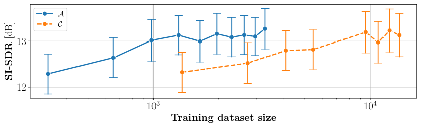
(a)

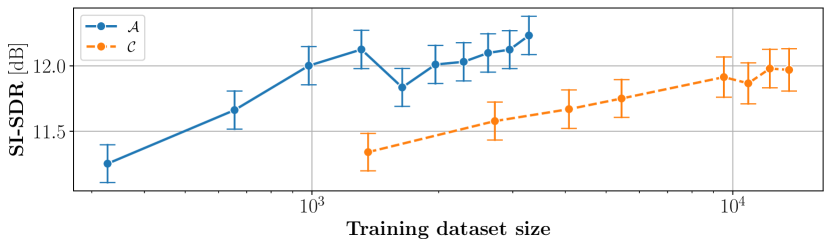
(b)

Fig. 2: SI-SDR mean and standard error for Vox-TasNet obtained training on different partitions of the two training datasets tested on MUSDB (a) and on $\mathcal{B}$ (b).

The final experiment aims at analysing the differences between the proposed Vox-TasNet stereo model and its mono version, MonoVox-TasNet. Both models have been trained on $\mathcal{A}$. In the first column of Table 3 we report SI-SDR computed separately on left and right channel, indicated as $\text{SI-SDR}^{\text{mono}}$. We verify that the difference between SI-SDR distributions for mono and stereo model on each evaluation dataset are not statistically significant, hence overall quality is not affected by stereo architecture. In the second column we report values for the stereo metric $\text{SSA}_{\text{SI-SDR}}$ proposed in Sec 2.2. A lower value indicates lower stereo artifacts and higher symmetry between left and right channel vocal attenuation. Results highlight that stereo architecture greatly improves output quality in terms of multichannel artifacts on both test datasets.

Model	Test Dataset	$\text{SI-SDR}^{\text{mono}}$ (dB)$\uparrow$	$\text{SSA}_{\text{SI-SDR}}$ (dB)$\downarrow$
Vox-TasNet	MUSDB	$12.79\pm 3.19$	$1.10\pm 0.45$
	$\mathcal{B}$	$11.64\pm 3.19$	$1.08\pm 0.58$
MonoVox-TasNet	MUSDB	$13.13\pm 2.94$	$1.81\pm 0.73$
	$\mathcal{B}$	$11.85\pm 3.21$	$2.30\pm 1.34$

Table 3: Mean and standard deviation of $\text{SI-SDR}^{\text{mono}}$ and of $\text{SSA}_{\text{SI-SDR}}$ for Vox-TasNet compared with the mono version trained on $\mathcal{A}$, tested on $\mathcal{B}$ and MUSDB. For $\text{SI-SDR}^{\text{mono}}$, the higher the better. For $\text{SSA}_{\text{SI-SDR}}$ the lower the better.

4.2 Subjective Evaluation

In Fig 3 we report MUSHRA scores for all conditions tested $\mathcal{I}$ and MUSDB. As expected, all models had lower scores than the reference audio on each evaluation dataset. Moreover, Vox-TasNet and MonoVox-TasNet had quality scores lower than HybridDemucs, but higher than the original Conv-TasNet architecture. Generally, models were perceived to have higher quality when tested on the MUSDB (vs. $\mathcal{I}$) dataset. Finally, while there was no meaningful difference between the mono and stereo models for the MUSDB dataset, Vox-TasNet had significantly better quality than MonoVox-TasNet on the $\mathcal{I}$ dataset.

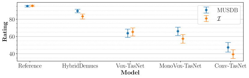
Fig. 3: Estimated MUSHRA scores for all conditions tested on $\mathcal{I}$ and MUSDB. Intervals are 95% credible intervals.

5 Conclusions

In this work we presented an efficient stereo SVC architecture, able to operate in real-time and with low memory requirements. By training the model on a large dataset, we reached performances comparable to larger and non-real-time models. Moreover, we show the benefits of using a stereo architecture through a new stereo separation asymmetry metric which can be formulated for any source separation metric. The results from objective evaluation are validated through a large-scale MUSHRA test. We believe this study may help in highlighting the key factors that enable the use of deep learning in real-time music processing.

References

- [1] M. Vardhana, N. Arunkumar, S. Lasrado, E. Abdulhay, and G. Ramirez-Gonzalez, “Convolutional neural network for bio-medical image segmentation with hardware acceleration,” Cognitive Systems Research, vol. 50, pp. 10–14, 2018.
- [2] A. Défossez, N. Usunier, L. Bottou, and F. Bach, “Music source separation in the waveform domain,” arXiv preprint arXiv:1911.13254, 2019.
- [3] R. Hennequin, A. Khlif, F. Voituret, and M. Moussallam, “Spleeter: a fast and efficient music source separation tool with pre-trained models,” Journal of Open Source Software, vol. 5, no. 50, pp. 2154, 2020.
- [4] Y. Luo and J. Yu, “Music source separation with band-split RNN,” IEEE/ACM Transactions on Audio, Speech, and Language Processing (TASLP), vol. 31, pp. 1893–1901, 2023.
- [5] W. Choi, M. Kim, J. Chung, and S. Jung, “LaSAFT: Latent source attentive frequency transformation for conditioned source separation,” in IEEE International Conference on Acoustics, Speech and Signal Processing (ICASSP), 2021.
- [6] N. Takahashi and Y. Mitsufuji, “D3net: Densely connected multidilated densenet for music source separation,” arXiv preprint arXiv:2010.01733, 2020.
- [7] D. Stoller, S. Ewert, and S. Dixon, “Wave-U-Net: A multi-scale neural network for end-to-end audio source separation,” in International Society for Music Information Retrieval Conference (ISMIR), 2018.
- [8] A. Défossez, “Hybrid spectrogram and waveform source separation,” in Proceedings of the MDX Workshop, 2021.
- [9] S. Rouard, F. Massa, and A. Défossez, “Hybrid transformers for music source separation,” in IEEE International Conference on Acoustics, Speech and Signal Processing (ICASSP), 2023.
- [10] W. Choi, M. Kim, J. Chung, D. Lee, and S. Jung, “Investigating U-nets with various intermediate blocks for spectrogram-based singing voice separation,” in International Society for Music Information Retrieval Conference (ISMIR), 2020.
- [11] X. Ni and J. Ren, “FC-U2-Net: A novel deep neural network for singing voice separation,” IEEE/ACM Transactions on Audio, Speech, and Language Processing (TASLP), vol. 30, pp. 489–494, 2022.
- [12] Y. Luo and N. Mesgarani, “Conv-TasNet: Surpassing ideal time–frequency magnitude masking for speech separation,” IEEE/ACM Transactions on Audio, Speech, and Language Processing (TASLP), vol. 27, no. 8, pp. 1256–1266, 2019.
- [13] Y. Hu, Y. Chen, W. Yang, L. He, and H. Huang, “Hierarchic temporal convolutional network with cross-domain encoder for music source separation,” IEEE Signal Processing Letters, vol. 29, pp. 1517–1521, 2022.
- [14] D. Samuel, A. Ganeshan, and J. Naradowsky, “Meta-learning extractors for music source separation,” in IEEE International Conference on Acoustics, Speech and Signal Processing (ICASSP), 2020.
- [15] A. Pandey and D. Wang, “TCNN: Temporal convolutional neural network for real-time speech enhancement in the time domain,” in IEEE International Conference on Acoustics, Speech and Signal Processing (ICASSP), 2019.
- [16] Z. Rafii, A. Liutkus, F.-R. Stöter, S. I. Mimilakis, and R. Bittner, “MUSDB18-HQ-an uncompressed version of MUSDB18,” https://doi.org/10.5281/zenodo.3338373.
- [17] D. P. Kingma and J. Ba, “Adam: A method for stochastic optimization,” arXiv preprint arXiv:1412.6980, 2014.
- [18] J. Le Roux, S. Wisdom, H. Erdogan, and J. R. Hershey, “SDR–half-baked or well done?,” in IEEE International Conference on Acoustics, Speech and Signal Processing (ICASSP), 2019.
- [19] E. Cano, D. FitzGerald, and K. Brandenburg, “Evaluation of quality of sound source separation algorithms: human perception vs quantitative metrics,” in European Signal Processing Conference (EUSIPCO), 2016.
- [20] B. Series, “Method for the subjective assessment of intermediate quality level of audio systems,” International Telecommunication Union Radiocommunication Assembly, 2014.
- [21] S. Ferrari and F. Cribari-Neto, “Beta regression for modelling rates and proportions,” Journal of applied statistics, vol. 31, no. 7, pp. 799–815, 2004.
- [22] M. Smithson and J. Verkuilen, “A better lemon squeezer? maximum-likelihood regression with beta-distributed dependent variables.,” Psychological methods, vol. 11, no. 1, pp. 54, 2006.
- [23] A. Gelman, J. B. Carlin, H. S. Stern, D. B. Dunson, A. Vehtari, and D. B. Rubin, Bayesian data analysis, Chapman and Hall/CRC, 2015.