Scaling Face Interaction Graph Networks to Real World Scenes

Abstract

Accurately simulating real world object dynamics is essential for various applications such as robotics, engineering, graphics, and design. To better capture complex real dynamics such as contact and friction, learned simulators based on graph networks have recently shown great promise (Allen et al., 2023; 2022). However, applying these learned simulators to real scenes comes with two major challenges: first, scaling learned simulators to handle the complexity of real world scenes which can involve hundreds of objects each with complicated 3D shapes, and second, handling inputs from perception rather than 3D state information. Here we introduce a method which substantially reduces the memory required to run graph-based learned simulators. Based on this memory-efficient simulation model, we then present a perceptual interface in the form of editable NeRFs which can convert real-world scenes into a structured representation that can be processed by graph network simulator. We show that our method uses substantially less memory than previous graph-based simulators while retaining their accuracy, and that the simulators learned in synthetic environments can be applied to real world scenes captured from multiple camera angles. This paves the way for expanding the application of learned simulators to settings where only perceptual information is available at inference time.

1 Introduction

Simulating rigid body dynamics is an important but challenging task with broad applications ranging from robotics to graphics to engineering. Widely used analytic rigid body simulators in robotics such as Bullet (Coumans, 2015), MuJoCo (Todorov et al., 2012), and Drake (Tedrake, 2019) can produce plausible predicted trajectories in simulation, but system identification is not always sufficient to bridge the gap between real world scenes and these simulators (Wieber et al., 2016; Stewart & Trinkle, 1996; Fazeli et al., 2017; Lan et al., 2022; Parmar et al., 2021; Guevara et al., 2017). This is due, in part, to the challenges of estimating fine-grained surface structures of objects which often have large impacts on their associated dynamics (Bauza & Rodriguez, 2017). This fundamental issue contributes to the well-documented sim-to-real gap between outcomes from analytical solvers and real-world experiments.

Learned simulators have shown the potential to fill the sim-to-real gap (Allen et al., 2023; 2022) by representing rigid body dynamics with graph neural networks. These fully learned simulators can be applied directly to real world object trajectories, and do not assume any analytical form for rigid body contacts. As a result, they can learn to be more accurate than system identification with an analytic simulator even with reasonably few real world trajectories.

However, real world scenes present major challenges for learned simulators. First, learned simulators generally assume access to full state information (the positions, rotations, and exact shapes of all objects) in order to simulate a trajectory. This information must be inferred from a collection of sensor measurements. Second, learned simulators can be memory intensive, especially for the kinds of intricate, irregular objects that often comprise real-world scenes. The currently best-performing graph-based methods operate on explicit surface representations, i.e. point clouds or triangulated meshes (Pfaff et al., 2021). The induced graphs of these methods tend to consume vast amounts of GPU memory for complex object geometries, or when there are many objects in the scene. Consequently, results are generally shown for scenes containing fewer than 10 objects with reasonably simple object geometries.

Here we propose a simple, yet surprisingly effective modification (FIGNet*) to the learned, mesh-based FIGNet rigid body simulator (Allen et al., 2023) that can address these challenges with representing and simulating real world scenes:

• FIGNet* consumes much less memory, while maintaining translation and rotation rollout accuracy. This allows us to train FIGNet* on datasets with more objects with complex geometries such as Kubric MOVi-C, which FIGNet cannot train on due to memory cost.

• We connect a NeRF perceptual front-end (Barron et al., 2022) to FIGNet*, and show that we can simulate plausible trajectories for complex, never-before-seen objects in real world scenes.

• We show that despite training FIGNet* on simulated rigid body dynamics with ground-truth meshes, the model is robust to noisy mesh estimates obtained from real-world NeRF data.

2 Related work

Learned simulators

attempt to replicate analytical simulators by employing a learned function approximator. Typically, they are trained using ground truth state information, and consequently cannot be directly applied to visual input data. The representation of state varies depending on the method, but can range from point clouds (Li et al., 2019; Sanchez-Gonzalez et al., 2020; Mrowca et al., 2018; Linkerhägner et al., 2023), to meshes (Pfaff et al., 2021; Allen et al., 2023), to signed distance functions (SDFs) (Le Cleac’h et al., 2023). Subsequently, learned function approximators such as multi-layer perceptrons (MLPs) (Li et al., 2021), graph neural networks (GNNs) (Battaglia et al., 2018; Sanchez-Gonzalez et al., 2018), or continuous convolutional kernels (Ummenhofer et al., 2019) can be employed to model the temporal evolution of the state. Our approach follows the mesh-based state representation options, but aims to provide a more efficient graph neural network dynamics model.

Bridging simulators to perception.

Multiple approaches aim to bridge these learned simulators to perceptual data. Some approaches are “end-to-end” – they train a perceptual input system jointly with a dynamics model, often assuming access to ground truth state information like object masks (Janner et al., 2019; Driess et al., 2022; Shi et al., 2022; Xue et al., 2023; Whitney et al., 2023). Others first learn a perceptual encoder and decoder, and then fix these to train a dynamics model in latent space (Li et al., 2021).

Most related to our approach are methods that use neural radiance fields to reconstruct 3D scenes from 2D multi-view scenes to enable simulation. Some of these assume hand-crafted but differentiable dynamics models (Qiao et al., 2023; 2022; Mengyu et al., 2022), while others learn the dynamics model separately from state information Guan et al. (2022). We similarly aim to simply apply our pre-trained learned simulators to real scenes by using a NeRF perceptual front-end. We show that this approach can work without fine-tuning even when simulators are trained only from synthetic data.

3 Method

3.1 FIGNet*

FIGNet* closely follows the method of Face Interaction Graph Networks (FIGNet) (Allen et al., 2023) which is a graph neural network approach designed for modeling rigid body dynamics. In FIGNet, each object is represented as a triangulated mesh $M$ made of triangular mesh faces $\{\mathcal{F}_{M}\}$ with mesh vertices $\{\mathcal{V}_{M}\}$. A scene graph $\mathcal{G}$ then consists of $O$ objects, each with their own triangulated meshes $M_{o}$. At any given time $t$, $M_{o}^{t}$ can be represented using the object’s transformation matrix, $M_{o}^{t}=R_{o}^{t}\times M_{o}$. A simulation trajectory is represented as a sequence of scene graphs $\mathcal{G}=(G^{t_{0}},G^{t_{1}},G^{t_{2}},\dots)$ constructed from these meshes. FIGNet is then a simulator $S$ parameterized by neural network weights $\Theta$, trained to predict the next state of the physical system $\tilde{G}^{t+1}$ based on the previous two scene graphs $\{G^{t},G^{t-1}\}$, ie $G^{t+1}=S_{\Theta}(G^{t},G^{t-1})$. We train with a mean-squared-error loss on the predicted positions of the vertices for each object $\{\mathcal{V}_{M}\}$. During inference, $S_{\Theta}$ can be recursively applied to yield a rollout of any length $T$.

Figure 1: Architectural changes: FIGNet* with respect to FIGNet.

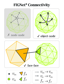
FIGNet consists of two types of nodes (mesh nodes $\{\mathcal{V}_{M}\}$ and object nodes $\{\mathcal{V}_{O}\}$), and three types of bi-directional edges.

The mesh nodes $\{\mathcal{V}_{M}\}$ have input features $\mathbf{v}^{\text{M,features}}_{i}=[\mathbf{x}^{t}_{i}-\mathbf{x}^{t-1}_{i},\mathbf{p}_{i},a_{i},\mathbf{f}^{t}_{i}]$, where $\mathbf{x}^{t}_{i}$ is the position of the node at time $t$, $\mathbf{p}_{i}$ are static object properties like density and friction, $a_{i}$ is a binary “static” feature that indicates whether the node is subject to dynamics (e.g. the moving objects), or its position is set externally (e.g. the floor), and $\mathbf{f}^{t}_{i}=k_{i}(\mathbf{x}^{t+1}_{i}-\mathbf{x}^{t}_{i})$ is a feature that indicates how much kinematic nodes are going to move at the next time step. Object nodes $\{\mathcal{V}_{O}\}$ use the same feature description, with their positions $\mathbf{x}^{t}_{i}$ being the object’s center of mass.

The three types of bi-directional edges include node-node, object-node, and face-face edges. Node-node edges $v_{m}\rightarrow v_{m}$ connect surface mesh nodes on a single object to one another. Object-node edges $v_{o}\rightarrow v_{m}$ connect object nodes $v_{o}$ to each mesh vertex $v_{m}$ of that object. Face-face edges connect faces on one sender object $f_{s}$ to another receiver object $f_{r}$. See Figure 1.

Conceptually, the node-node edges enable the propagation of messages locally along an object’s surface. However, in the case of rigid body collisions, collision information needs to be propagated instantaneously from one side of the object to the other, irrespective of the mesh complexity. Object-node edges enable this by having a single virtual object node $v_{o}$ at the center of each object which has bidirectional edges to each mesh node $v_{m}$ on the object’s surface. Finally, to model the collision dynamics between rigid objects, face-face edges convey information about face interactions between objects. FIGNet proposes a special hypergraph architecture for how to incorporate face-face edges into an Encode-Process-Decode graph network architecture. We defer further details of the FIGNet approach to (Allen et al., 2023).

This approach works remarkably well for rigid body shapes but becomes intractably expensive as the complexity of each object mesh grows, since this will add a significant number of node-node (surface mesh) edges. Empirically, node-node edges often account for more than 50$\%$ of the total edges in FIGNet. FIGNet* makes a simple modification to FIGNet which removes the node-node (surface mesh) edges, keeping everything else identical. Surprisingly, this does not hurt the accuracy of FIGNet*, but dramatically improves memory and runtime performance for the rigid body settings examined in this paper. This works for rigid body dynamics because the collision edges reason about the local geometry of two objects involved in contact, and this information can then be directly broadcasted to the whole shape using object-node edges.

This simple change to FIGNet unlocks the ability to train on much more complex scenes than was previously possible, as larger scenes fit into accelerator memory during training. We can therefore run FIGNet* on meshes extracted from real-world scenes, as well as simulations with more complex object geometries than previously possible.

3.2 Connecting FIGNet* to Perception

In this section we describe the procedure used to connect FIGNet* to the real world. We leverage Neural Radiance Fields (NeRFs) (Mildenhall et al., 2021; Barron et al., 2022) as a perceptual front end to (1) extract the meshes required by FIGNet* for simulation and (2) re-render the scene with the transformations predicted by FIGNet* (Figure 2). This approach shares similarities with the method presented in (Qiao et al., 2023), however, here we demonstrate its implementation using a learned simulator.

Figure 2: Perception Pipeline. We demonstrate a two-way coupling approach, integrating FIGNet* with real-world scenes through NeRF. Initially, a static NeRF scene is trained using a collection of images capturing a real-world scene, enabling the extraction of the necessary meshes for FIGNet*. Upon obtaining the rollout trajectory, we derive a set of rigid body transformations, which are then utilized to edit the original NeRF. See subsection 3.2 for details.

3.2.1 From NeRF to FIGNet*

Learning a Neural Radiance Field:

We first learn a NeRF from $W$ sparse input views $\{I\}_{1}^{W}$ and their associated camera intrinsics $\mathbf{K}$ and extrinsics. This representation models a view-dependent appearance function $F_{\Phi}$ that maps a 3D location $\mathbf{x}=(x,y,z)$ and a viewing direction $\mathbf{d}$ to a radiance color $\mathbf{c}$ and a density $\sigma$.

$$F_{\Phi}:(\mathbf{x},\mathbf{d})\to(\mathbf{c},\sigma)$$ (1)

The geometries of all the objects in a scene represented by a NeRF are implicitly captured by $F_{\Phi}$. We only care about the density $\sigma$ for the geometry and can ignore the color $\mathbf{c}$ and the viewing direction $\mathbf{d}$. We slightly abuse the notation and define $F_{\Phi}^{\sigma}(\mathbf{x})\to\sigma$ to denote the subpart of the NeRF that evaluates the density only.

Mesh Extraction:

To extract the mesh of an individual object from the implicit function $F_{\Phi}^{\sigma}$, we first need to define a volumetric boundary of the object.

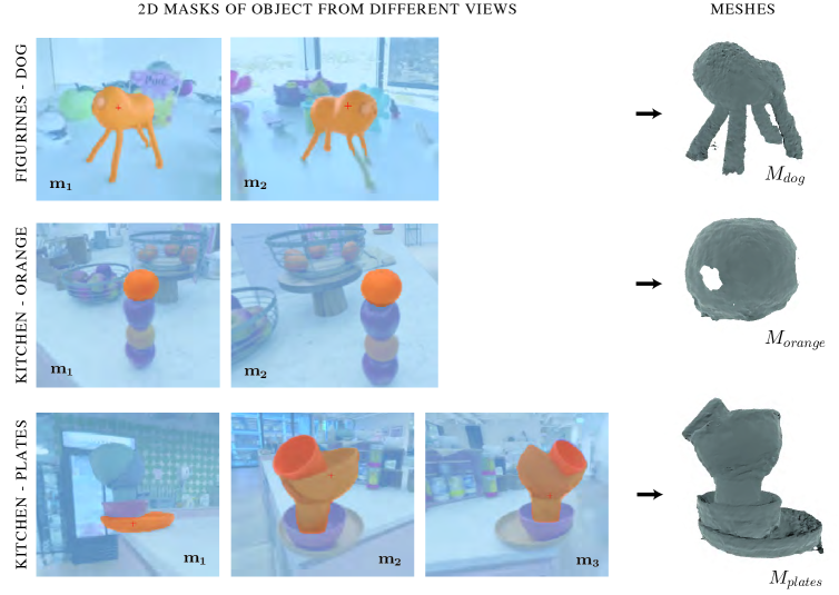
We begin by generating $N$ binary segmentation masks, each capturing the object’s shape from one of $N$ distinct viewpoints. Each mask is created by calling XMEM (Cheng & Schwing, 2022) with the corresponding RGB image and a point prompt located at the center of the object. XMEM then identifies and labels all active pixels belonging to the object in each mask at the prompted location, resulting in a set of N segmentation masks $\{\mathbf{m_{n}}\}_{1}^{N}$ that capture the object’s shape from various perspectives. Empirically, we found that for simple objects like spheres, as few as two views from different angles are sufficient to accurately segment the object. However, one can use additional views for increased robustness or to capture finer details, particularly for more complex shapes.

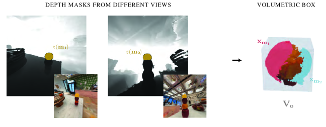
We use the same procedure as described in (Cen et al., 2023) to unproject the pixels of the 2D masks into 3D points by leveraging the estimated depth $z(\mathbf{m_{n}})$ from the NeRF and the known camera intrinsics from which each mask was generated:

$$\mathbf{x}_{\mathbf{m_{n}}}=z(\mathbf{m_{n}})*\mathbf{K}^{-1}\cdot(x(\mathbf{m_{n}}),y(\mathbf{m_{n}}),1)^{T}$$ (2)

The volumetric boundary $\mathbf{V_{o}}\in\mathbb{R}^{2\times 3}$ can be then obtained as

$$\mathbf{V_{o}}=\{\min(\mathbf{x}_{\mathbf{m_{n}}}),\max(\mathbf{x}_{\mathbf{m_{n}}})\}_{1}^{N}$$ (3)

To extract the mesh of the object $M_{o}$ within the volume $\mathbf{V_{o}}$, we employ the Marching Cubes algorithm (m_cubes) (Lorensen & Cline, 1998). This algorithm uses samples of the density field from a regular grid of J points inside the boundary $\mathbf{x}_{j}\in\mathbf{V_{o}}$ as $\mathbf{\sigma_{o}}=\{F_{\Phi}^{\sigma}(\mathbf{x}_{j})\}_{1}^{J}$ and a threshold value $\sigma_{thrs}$. To manage the potentially high number of vertices and faces in the generated mesh, we perform an additional decimation step (decimate). We employ the Quadric Error Metric Decimation method by Garland and Heckbert (Garland & Heckbert, 1997). This technique preserves the primary features of the mesh while allowing us to control the final mesh complexity through a user-specified target number of faces $n_{f}$.

$$M_{o}=\texttt{decimate}(\,\texttt{m\_cubes}(\mathbf{\sigma_{o}},\sigma_{thrs}),\,n_{f})$$ (4)

Building the Graph

To specify the object whose motion we want to simulate, we define the mesh $M_{o}$ as the active object in the graph, with all other objects considered static. We then repeat the same mesh extraction procedure described above on an offset version of the scene volume $(\mathbf{V_{o}}-\Delta\mathbf{x}_{\mathbf{V_{o}}})$ to obtain the passive mesh $M_{passive}$ representing the static environment with $a_{i}$ set to True. Both meshes are used to construct the initial graph $G^{t}$ for FIGNet and FIGNet*. We do not infer static properties like mass, friction, elasticity, etc for meshes extracted from the scene. Instead we use the default parameters provided in Table 3. Future work will be needed to infer these properties from object dynamics.

We generate the history $G^{t-1}$ using the same mesh but shifted downwards by a $\Delta z$ amount twice to simulate an object being dropped vertically.

3.2.2 From FIGNet* to NeRF

We obtain a rollout trajectory by iteratively applying FIGNet* over $T$ time steps. Starting from the initial graph and its history to obtain $(G^{t+1},G^{t+2},\cdots,G^{t+T})$. This can be equivalently seen as a sequence of rigid transformations $(R_{o}^{t+1},R_{o}^{t+2},\cdots,R_{o}^{t+T})$ that are applied to $M_{o}$.

Given the bounding volume of each object $\mathbf{V_{o}}$ and a rigid transformation $R_{t}$ at time $t$, we can reuse the static NeRF function $F_{\Phi}$ to render the rollout by editing the original static NeRF described by $F_{\Phi}$ via ray bending (Jambon et al., 2023). We restrict the bending of the ray $b$ to be the rigid transformation returned by FIGNet* as

$$\hat{F_{\Phi}}:(\,b(\mathbf{x},R_{o}^{t}\,),\mathbf{d})\to(\mathbf{c},\sigma),$$ (5)

where $b(\mathbf{x},R_{o}^{t}\,)$ can be either

$$b_{move}(\mathbf{x},R_{o}^{t})=\begin{cases}R_{o}^{t}\times\mathbf{x}&\quad\text{if }\mathbf{x}\in\mathbf{V_{o}}\text{,}\\ (R_{o}^{t})^{-1}\times\mathbf{x}&\quad\text{if }\mathbf{x}\in R_{o}^{t}\times\mathbf{V_{o}}\text{,}\\ \mathbf{x}&\quad\text{otherwise.}\\ \end{cases}$$ (6)

or

$$b_{duplicate}(\mathbf{x},R_{o}^{t})=\begin{cases}(R_{o}^{t})^{-1}\times\mathbf{x}&\quad\text{if }\mathbf{x}\in R_{o}^{t}\times\mathbf{V_{o}}\text{,}\\ \mathbf{x}&\quad\text{otherwise.}\\ \end{cases}$$ (7)

meaning that the active object has the option to be either moved or copy-pasted during the rollout.

We then generate the final sequence of rollout images from a chosen viewpoint $\hat{\mathbf{d}}$ across all time steps. This involves applying NeRF’s classic volume rendering pipeline with the transformed radiance field $\hat{F_{\Phi}}$ incorporating object movement. At each step, we adjust the radiance field based on the applied rigid transformation, effectively capturing the dynamic appearance of the object throughout the rollout sequence $\{\hat{F_{\Phi}}(b(\mathbf{x},R_{t}\,),\hat{\mathbf{d}})\}_{t=1}^{k}$.

4 Results

We test FIGNet* on both simulated and real data. In simulation, we show that FIGNet* outperforms FIGNet in memory consumption and runtime while maintaining accuracy for a standard rigid body dynamics benchmark (Greff et al., 2022). For real data, we show that FIGNet* can be run on views of real scenes collected from multiple cameras, making plausible trajectories despite training in simulation on perfect state information.

4.1 Simulation

For our simulation results, we use the MOVi-B and MOVi-C Kubric datasets (Greff et al., 2022). In both setups, multiple rigid objects are tossed together onto the floor using the PyBullet (Coumans) simulator to predict trajectories. MOVi-B consists of scenes involving 3-10 objects selected from 11 different shapes being tossed. The shapes include teapots, gears, and torus knots, with a few hundred up to just over one thousand vertices per object. MOVi-C consists of scenes involving 3-10 objects selected from 1030 different shapes taken from the Google Scanned Objects dataset (Downs et al., 2022). MOVi-C shapes tend to be more complex than MOVi-B shapes, and have up to several thousand or tens of thousands of vertices.

We report four metrics in Table 2: peak memory consumption, runtime per simulation step, translation error, and rotation error. Translation and rotation root-mean-squared error (RMSE) are calculated with respect to the ground truth state after 50 rollout steps.

Table 1: Comparison metrics for FIGNet and FIGNet* on Kubric MOVi-B and MOVi-C

Dataset	Model	Memory (MiB)	Runtime (ms)	Trans. Err. (m)	Rot. Err. (deg)	Edge Count ($\#$)
MOVi-B	FIGNet	63.38 $\pm$ 3.32	26.38 $\pm$ 0.73	0.14 $\pm$ 0.01	14.99 $\pm$ 0.67	24514 $\pm$ 906
	FIGNet*	50.08 $\pm$ 3.37	19.41 $\pm$ 0.24	0.13 $\pm$ 0.01	15.96 $\pm$ 0.87	8630 $\pm$ 714
MOVi-C	FIGNet	OOM	–	–	–	–
	FIGNet*	71.79 $\pm$ 6.39	20.42 $\pm$ 0.64	0.18 $\pm$ 0.01	19.82 $\pm$ 0.64	11401 $\pm$ 975

For MOVi-B, FIGNet* matches FIGNet’s performance in translation and rotation error, performing slightly better in translation, and slightly worse on rotation. However, FIGNet* uses significantly less memory than FIGNet while also having a 20$\%$ faster runtime. These differences in memory consumption and runtime allow us to train FIGNet* on the much more complex MOVi-C dataset (example trajectory in Figure 3), which causes OOM errors when attempting to train FIGNet even with 16 A100 GPUs. On MOVi-C, the memory consumption is higher, but runtime remains almost as fast. Similarly, since MOVi-C is more complex than MOVi-B, the translation and rotation errors for FIGNet* are higher, but not significantly so.

Overall, this suggests that FIGNet* is a viable alternative to FIGNet. It maintains accuracy while significantly reducing memory consumption and runtime, allowing us to train FIGNet* on more complex datasets than can be fit into FIGNet memory.

Ground
truth

FIGNet*

Figure 3: Qualitative results for simulation. FIGNet* rollout for complex MOVi-C simulation which could not be represented in memory for FIGNet.

4.2 Real world

We present our results on linking FIGNet* with real-world scene inputs. Note that this is a proof-of-concept only, that is we do not compare to real ground truth dynamics, instead leaving that for future work. For comparisons between FIGNet and FIGNet* on real data, FIGNet models were trained in simulation on Kubric MOVi-B, while FIGNet* models were trained in simulation on Kubric MOVi-C.

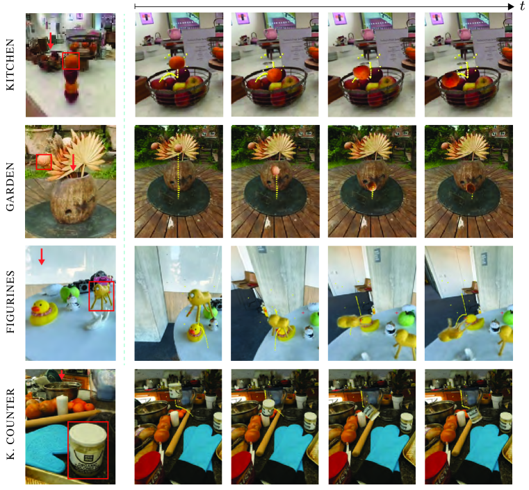
For our real-world results, we used two scenes: our custom-made kitchen scene filled with common elements such as fruits and baskets (See Appendix C for details), the garden-outdoor and kitchen counter-indoor scenes introduced in (Barron et al., 2022) and the figurines scene introduced in (Kerr et al., 2023). These scenes consist of 360-degree image sets captured with different cameras. We used a MipNerf360 (Barron et al., 2022) implementation for the NeRF front end.

Figure 4: Qualitative results for real world scenes. Left: Initial NeRF rendering of the static real-world scene. The desired active object is outlined in red, with a red arrow indicating its intended starting position. Right: FIGNet* rollouts simulating the object’s motion for $k=30$ time steps (rendered from a different viewpoint) after being dropped from the initial position. The complete trajectory is traced in yellow. Here we used $b_{duplicate}$ as the ray bending function meaning the active object is copy pasted into the starting position at the beginning of the rollout (See the website for videos and Appendix B for details on the mesh extraction procedure described in subsection 3.2).

Qualitative Results.

We show qualitative FIGNet* rollouts on both real world scenes using the full pipeline described in subsection 3.2. For all the scenes, we manually selected 2 views of the active object (highlighted in the red boxes) to compute the bounding volume $\mathbf{V_{o}}$ and the subsequent mesh $M_{o}$ (See Appendix B). By creating a history based on downward vertical displacement of the chosen mesh, we are effectively simulating a motion similar to dropping. Figure 4 illustrates the bouncing behaviors of various objects falling onto other objects. Note the sharp rotation of the orange at the end of the bounce (last frame) in the kitchen scene, and how rendering with the transformed $\hat{F_{\Phi}}$ works when the orange is flipped upside down. We can observe similar results for the figurines scene, where we selected two views of the dog figurine with long thing legs and simulate a dropping motion onto a duck. Our perception pipeline can realistically simulate and re-render the dropping motion of objects captured within these real scenes by reusing the static NeRF scene with the FIGNet* transformations .

Figure 5: FIGNet and FIGNet* comparison for different levels of decimation: High-quality meshes lead to out-of-memory issues on FIGNet, while lower resolutions result in implausible trajectories (e.g., orange penetrating the basket). Notably, FIGNet*’s performance gracefully degrades with mesh quality, indicating enhanced robustness and memory efficiency. The gray mesh depicts the passive object, and the colored mesh corresponds to the active object.

Effect of decimation.

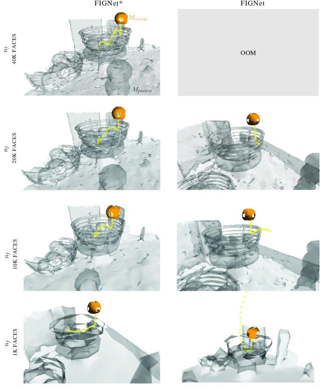
The marching cube algorithm often results in oversampled meshes characterized by an elevated node count. While the implementation of a controllable parameter for mesh decimation ($n_{f}$) is an effective strategy to address this challenge, it is important to note that the extent of decimation can adversely affect the quality of simulations, especially in cases involving complex geometries. The advantage of using FIGNet* lies in its reduced memory requirements, which permits a less rigorous decimation process in comparison to FIGNet. To demonstrate this, we simulated a scene with two distinct levels of decimation (Figure 5). This experiment highlights instances where FIGNet’s memory capacity is exceeded, showcasing the benefits of FIGNet* in such scenarios.

Effect of perception noise.

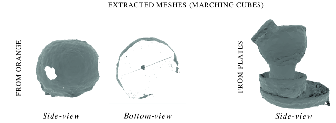
Real-world meshes extracted from pipelines like NeRF, primarily optimized for rendering quality, often exhibit noise and imperfections (Figure 6). Unlike the clean training data used for FIGNet* and FIGNet, these meshes are far from ideal. Nevertheless, both models can successfully handle rollouts even with such challenging real-world data.

5 Discussion

We showed that a surprisingly simple modification to FIGNet, the removal of the surface mesh edges, allowed us to create a model with low enough memory consumption to support training on unprecedentedly complex scenes. This unlocked the ability to interface FIGNet* with real world scenes by using a combination of Neural Radiance Fields (NeRFs) and object selection (XMem) to convert real scenes into object-based mesh representations. In combination with volumetric NeRF editing, this allowed us to simulate videos of alternative physical futures for real scenes.

We believe that this explicitly 3D approach to video editing and generation has significant promise for robotics and graphics applications. It allows a model to be pre-trained from simulation data, while still generalizing to real scenes. FIGNet* generalizes surprisingly well to noisy meshes extracted from NeRFs, especially considering that it was trained in simulation with nearly perfect state information (positions, rotations, and shapes of objects). We imagine that this approach could further support future applications including “virtualization” of real scenes, where users may be interested in editing those scenes and simulating possible future outcomes.

There are many exciting directions for future work with FIGNet*. In particular, while fine-tuning a pre-trained FIGNet* model to a real video was outside the scope of this paper, we believe this is a natural next step. Since FIGNet* is entirely composed of neural networks, fine-tuning from real world dynamics directly into the weights of FIGNet* could be a viable alternative to system identification for robotics. Future work will be needed to determine the details of how to perform fine-tuning in a data efficient manner.

Appendix

Appendix A Decimation experiments

We qualitatively evaluated the impact of mesh decimation on rollouts for FIGNet and FIGNet* in the kitchen scene (Figure 5). With higher quality meshes (lower decimation), FIGNet tends to run out of memory, whereas lower quality meshes (higher decimation) often result in unrealistic rollouts. In such cases, objects (orange) may pass through solid objects (basket), as observed with meshes of 1k faces. In contrast, FIGNet*’s rollout trajectories exhibit a graceful degradation with increased levels of decimation, maintaining relative stability even at very high decimation levels ($n_{f}=1000$, which means approximately 1% of the original faces are preserved)

Figure 6: Noisy meshes extracted from NeRF, including the orange object on the left missing its bottom face (from Figure 4) and the plates (from Figure 11). Notably, both FIGNet and FIGNet* can handle rollouts even with such mesh imperfections, demonstrating their robustness to real-world data challenges.

Figure 7: Effect of the decimation parameter on the mesh quality. Left: no decimation. Right: high decimation.

Appendix B Image segmentations

We provide some examples of how the mesh extraction procedure described in subsection 3.2 works in Figure 8 and Figure 9.

Figure 8: Left: Selected views to generate the objects masks for the figurines and kitchen scenes. The top row corresponds to the rendered image in RGB with each orange mask $\{\mathbf{m_{n}}\}_{1}^{N}$ (overlaid in light orange) obtained by XMEM’s (Cheng & Schwing, 2022). The bottom row illustrates the same procedure for the plates on the same scene. Note that partial segmentations from different views can also be used to build the volumetric boundary of the object. Right: the obtained mesh $M_{o}$ from each of the masks after decimation.

Figure 9: Visualizing the generation of the orange’s volumetric box from depth masks in the kitchen scene.

Appendix C Kitchen scene details

We collected 1027 images of a kitchen scene that included different elements such as apples, oranges, baskets and plates. We extracted the images from a video recorded with an iPhone 14 Pro at 60fps and HEVC format (Figure 10). We used COLMAP (Schonberger & Frahm, 2016) to estimate the camera poses from the images.

Figure 10: Example frames from the kitchen scene video.

Appendix D Implementation details

D.1 Hyper-parameters

FIGNet* is trained identically to FIGNet (Allen et al., 2023).

MLPs for Encoder, Processor, Decoder

We use MLPs with 2 hidden layers, and 128 hidden and output sizes (except the decoder MLP, with an output size of 3). All MLPs, except for those in the decoder, are followed by a LayerNorm(Ba et al., 2016) layer.

Optimization

All models are trained to 1M steps with a batch size of 128 across 8 TPU devices. We use Adam optimizer, and an an exponential learning rate decay from 1e-3 to 1e-4.

Table 2: NeRF Training Parameters

Type	Parameter	Value
General	near	0.
General	far	1e6
General	lr_delay_steps	100
General	batch_size	65536
General	lr_init	1e-2
General	lr_final	1e-3
General	adam_beta1	0.9
General	adam_beta2	0.99
General	adam_eps	1e-15
General	cast_rays_in_eval_step	True
General	cast_rays_in_train_step	True
General	num_glo_features	4
Model	sampling_strategy	((0, 0, 64), (0, 0, 64), (1, 1, 32))
Model	grid_params_per_level	(1, 4)
Hash	hash_map_size	2097152
Hash	scale_supersample	1.
Hash	max_grid_size	8192
MLP	net_depth	1
MLP	net_width	64
MLP	disable_density_normals	True
MLP	density_activation	@math.safe_exp
MLP	bottleneck_width	15
MLP	net_depth_viewdirs	2
MLP	net_width_viewdirs	64

Table 3: Default Physical Parameters

Model	Type	Mass	Friction	Restitution
FIGNet*	Active	1e-3	0.5	0.5
FIGNet*	Passive	0	0.5	0.3
FIGNet	Active	1.0	0.8	0.7
FIGNet	Passive	0	0.5	0.3

Appendix E Additional rollouts for the real world scenes

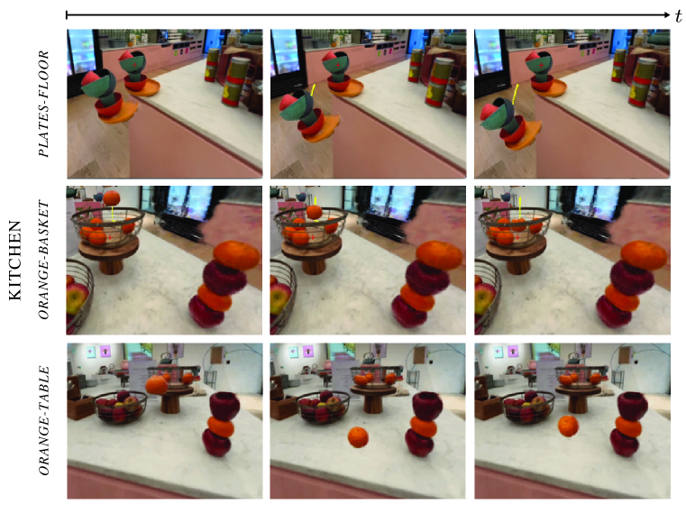
We provide additional rollout examples for the kitchen scene in Figure 11 and in the website. plates-floor: Duplicating the stack of plates on the right and shifting their initial position to the left. orange-basket: The top orange from the stack of fruits is duplicated and dropped on top of a basket of oranges. Note the correct depth ordering of the orange with respect to the basket. orange-table: the orange is dropped on the table.

Figure 11: Additional examples of FIGNet* rollouts on the kitchen scene. The final row was generated using the $b_{move}$ ray bending function (moving the orange from the fruit tower to the starting position), while the other rows used $b_{duplicate}$ (copy-pasting the object).

Appendix F Example rollouts for MOVi-C

Additional simulation rollouts of FIGNet* on Kubric MOVI-C.

Ground
truth

FIGNet*

Ground
truth

FIGNet*

Ground
truth

FIGNet*

Figure 12: Rollout of FIGNet* Kubric MOVi-C.

References

- Allen et al. (2022) Kelsey R Allen, Tatiana Lopez Guevara, Yulia Rubanova, Kim Stachenfeld, Alvaro Sanchez-Gonzalez, Peter Battaglia, and Tobias Pfaff. Graph network simulators can learn discontinuous, rigid contact dynamics. In 6th Annual Conference on Robot Learning, 2022. URL https://openreview.net/forum?id=rbIzq-I84i_.
- Allen et al. (2023) Kelsey R. Allen, Yulia Rubanova, Tatiana Lopez-Guevara, William Whitney, Alvaro Sanchez-Gonzalez, Peter Battaglia, and Tobias Pfaff. Learning rigid dynamics with face interaction graph networks. In International Conference on Learning Representations, 2023.
- Ba et al. (2016) Jimmy Lei Ba, Jamie Ryan Kiros, and Geoffrey E Hinton. Layer normalization. arXiv preprint arXiv:1607.06450, 2016.
- Barron et al. (2022) Jonathan T. Barron, Ben Mildenhall, Dor Verbin, Pratul P. Srinivasan, and Peter Hedman. Mip-nerf 360: Unbounded anti-aliased neural radiance fields. CVPR, 2022.
- Battaglia et al. (2018) Peter W Battaglia, Jessica B Hamrick, Victor Bapst, Alvaro Sanchez-Gonzalez, Vinicius Zambaldi, Mateusz Malinowski, Andrea Tacchetti, David Raposo, Adam Santoro, Ryan Faulkner, et al. Relational inductive biases, deep learning, and graph networks. arXiv preprint arXiv:1806.01261, 2018.
- Bauza & Rodriguez (2017) Maria Bauza and Alberto Rodriguez. A probabilistic data-driven model for planar pushing. In IEEE International Conference on Robotics and Automation (ICRA), pp. 3008–3015, 2017.
- Cen et al. (2023) Jiazhong Cen, Zanwei Zhou, Jiemin Fang, Chen Yang, Wei Shen, Lingxi Xie, Dongsheng Jiang, Xiaopeng Zhang, and Qi Tian. Segment anything in 3d with nerfs. In NeurIPS, 2023.
- Cheng & Schwing (2022) Ho Kei Cheng and Alexander G. Schwing. XMem: Long-term video object segmentation with an atkinson-shiffrin memory model. In ECCV, 2022.
- Coumans (2015) Erwin Coumans. Bullet physics simulation. In ACM SIGGRAPH 2015 Courses, pp. 7, 2015.
- Downs et al. (2022) Laura Downs, Anthony Francis, Nate Koenig, Brandon Kinman, Ryan Hickman, Krista Reymann, Thomas B McHugh, and Vincent Vanhoucke. Google scanned objects: A high-quality dataset of 3d scanned household items. arXiv preprint arXiv:2204.11918, 2022.
- Driess et al. (2022) Danny Driess, Zhiao Huang, Yunzhu Li, Russ Tedrake, and Marc Toussaint. Learning multi-object dynamics with compositional neural radiance fields. arXiv preprint arXiv:2202.11855, 2022.
- Fazeli et al. (2017) Nima Fazeli, Elliott Donlon, Evan Drumwright, and Alberto Rodriguez. Empirical evaluation of common contact models for planar impact. In 2017 IEEE international conference on robotics and automation (ICRA), pp. 3418–3425. IEEE, 2017.
- Garland & Heckbert (1997) Michael Garland and Paul S Heckbert. Surface simplification using quadric error metrics. In Proceedings of the 24th annual conference on Computer graphics and interactive techniques, pp. 209–216, 1997.
- Greff et al. (2022) Klaus Greff, Francois Belletti, Lucas Beyer, Carl Doersch, Yilun Du, Daniel Duckworth, David J Fleet, Dan Gnanapragasam, Florian Golemo, Charles Herrmann, et al. Kubric: A scalable dataset generator. In Proceedings of the IEEE/CVF Conference on Computer Vision and Pattern Recognition, pp. 3749–3761, 2022.
- Guan et al. (2022) Shanyan Guan, Huayu Deng, Yunbo Wang, and Xiaokang Yang. Neurofluid: Fluid dynamics grounding with particle-driven neural radiance fields, 2022.
- Guevara et al. (2017) Tatiana López Guevara, Nicholas Kenelm Taylor, Michael Gutmann, Subramanian Ramamoorthy, and Kartic Subr. Adaptable pouring: Teaching robots not to spill using fast but approximate fluid simulation. In 1st Conference on Robot Learning 2017, pp. 77–86, 2017.
- Jambon et al. (2023) Clément Jambon, Bernhard Kerbl, Georgios Kopanas, Stavros Diolatzis, George Drettakis, and Thomas Leimkühler. Nerfshop: Interactive editing of neural radiance fields. Proceedings of the ACM on Computer Graphics and Interactive Techniques, 6(1), 2023.
- Janner et al. (2019) Michael Janner, Sergey Levine, William T. Freeman, Joshua B. Tenenbaum, Chelsea Finn, and Jiajun Wu. Reasoning about physical interactions with object-oriented prediction and planning, 2019.
- Kerr et al. (2023) Justin Kerr, Chung Min Kim, Ken Goldberg, Angjoo Kanazawa, and Matthew Tancik. Lerf: Language embedded radiance fields. In International Conference on Computer Vision (ICCV), 2023.
- Lan et al. (2022) Lei Lan, Danny M Kaufman, Minchen Li, Chenfanfu Jiang, and Yin Yang. Affine body dynamics: Fast, stable & intersection-free simulation of stiff materials. ACM Trans. Graph, 2022.
- Le Cleac’h et al. (2023) Simon Le Cleac’h, Hong-Xing Yu, Michelle Guo, Taylor Howell, Ruohan Gao, Jiajun Wu, Zachary Manchester, and Mac Schwager. Differentiable physics simulation of dynamics-augmented neural objects. IEEE Robotics and Automation Letters, 8(5):2780–2787, 2023.
- Li et al. (2019) Yunzhu Li, Jiajun Wu, Russ Tedrake, Joshua B. Tenenbaum, and Antonio Torralba. Learning particle dynamics for manipulating rigid bodies, deformable objects, and fluids. In International Conference on Learning Representations, 2019.
- Li et al. (2021) Yunzhu Li, Shuang Li, Vincent Sitzmann, Pulkit Agrawal, and Antonio Torralba. 3d neural scene representations for visuomotor control. arXiv preprint arXiv:2107.04004, 2021.
- Linkerhägner et al. (2023) Jonas Linkerhägner, Niklas Freymuth, Paul Maria Scheikl, Franziska Mathis-Ullrich, and Gerhard Neumann. Grounding graph network simulators using physical sensor observations. arXiv preprint arXiv:2302.11864, 2023.
- Lorensen & Cline (1998) William E Lorensen and Harvey E Cline. Marching cubes: A high resolution 3d surface construction algorithm. In Seminal graphics: pioneering efforts that shaped the field, pp. 347–353. 1998.
- Mengyu et al. (2022) Chu Mengyu, Liu Lingjie, Zheng Quan, Franz Erik, Seidel Hans-Peter, Theobalt Christian, and Zayer Rhaleb. Physics informed neural fields for smoke reconstruction with sparse data. ACM Transactions on Graphics, 41(4):119:1–119:14, aug 2022.
- Mildenhall et al. (2021) Ben Mildenhall, Pratul P Srinivasan, Matthew Tancik, Jonathan T Barron, Ravi Ramamoorthi, and Ren Ng. Nerf: Representing scenes as neural radiance fields for view synthesis. Communications of the ACM, 65(1):99–106, 2021.
- Mrowca et al. (2018) Damian Mrowca, Chengxu Zhuang, Elias Wang, Nick Haber, Li F Fei-Fei, Josh Tenenbaum, and Daniel L Yamins. Flexible neural representation for physics prediction. Advances in neural information processing systems, 31, 2018.
- Parmar et al. (2021) Mihir Parmar, Mathew Halm, and Michael Posa. Fundamental challenges in deep learning for stiff contact dynamics. In 2021 IEEE/RSJ International Conference on Intelligent Robots and Systems (IROS), pp. 5181–5188. IEEE, 2021.
- Pfaff et al. (2021) Tobias Pfaff, Meire Fortunato, Alvaro Sanchez-Gonzalez, and Peter Battaglia. Learning mesh-based simulation with graph networks. In International Conference on Learning Representations, 2021.
- Qiao et al. (2022) Yi-Ling Qiao, Alexander Gao, and Ming C. Lin. Neuphysics: Editable neural geometry and physics from monocular videos. In Conference on Neural Information Processing Systems (NeurIPS), 2022.
- Qiao et al. (2023) Yi-Ling Qiao, Alexander Gao, Yiran Xu, Yue Feng, Jia-Bin Huang, and Ming C. Lin. Dynamic mesh-aware radiance fields. ICCV, 2023.
- Sanchez-Gonzalez et al. (2018) Alvaro Sanchez-Gonzalez, Nicolas Heess, Jost Tobias Springenberg, Josh Merel, Martin Riedmiller, Raia Hadsell, and Peter Battaglia. Graph networks as learnable physics engines for inference and control. In International Conference on Machine Learning, pp. 4470–4479. PMLR, 2018.
- Sanchez-Gonzalez et al. (2020) Alvaro Sanchez-Gonzalez, Jonathan Godwin, Tobias Pfaff, Rex Ying, Jure Leskovec, and Peter Battaglia. Learning to simulate complex physics with graph networks. In International Conference on Machine Learning, pp. 8459–8468. PMLR, 2020.
- Schonberger & Frahm (2016) Johannes L Schonberger and Jan-Michael Frahm. Structure-from-motion revisited. In Proceedings of the IEEE conference on computer vision and pattern recognition, pp. 4104–4113, 2016.
- Shi et al. (2022) Haochen Shi, Huazhe Xu, Zhiao Huang, Yunzhu Li, and Jiajun Wu. Robocraft: Learning to see, simulate, and shape elasto-plastic objects with graph networks, 2022.
- Stewart & Trinkle (1996) D Stewart and JC J.C. Trinkle. An implicit time-stepping scheme for rigid body dynamics with Coulomb friction. International Journal for Numerical Methods in Engineering, 39(15):2673–2691, 1996.
- Tedrake (2019) Russ Tedrake. Drake: Model-based design and verification for robotics, 2019. URL https://drake.mit.edu.
- Todorov et al. (2012) Emanuel Todorov, Tom Erez, and Yuval Tassa. Mujoco: A physics engine for model-based control. In 2012 IEEE/RSJ international conference on intelligent robots and systems, pp. 5026–5033. IEEE, 2012.
- Ummenhofer et al. (2019) Benjamin Ummenhofer, Lukas Prantl, Nils Thuerey, and Vladlen Koltun. Lagrangian fluid simulation with continuous convolutions. In International Conference on Learning Representations, 2019.
- Whitney et al. (2023) William F. Whitney, Tatiana Lopez-Guevara, Tobias Pfaff, Yulia Rubanova, Thomas Kipf, Kimberly Stachenfeld, and Kelsey R. Allen. Learning 3d particle-based simulators from rgb-d videos, 2023.
- Wieber et al. (2016) Pierre-Brice Wieber, Russ Tedrake, and Scott Kuindersma. Modeling and control of legged robots. In Springer handbook of robotics, pp. 1203–1234. Springer, 2016.
- Xue et al. (2023) Haotian Xue, Antonio Torralba, Joshua B. Tenenbaum, Daniel LK Yamins, Yunzhu Li, and Hsiao-Yu Tung. 3d-intphys: Towards more generalized 3d-grounded visual intuitive physics under challenging scenes, 2023.