Numerical Solutions for Stochastic Continuous-time Algebraic Riccati Equations

Abstract

We are concerned with efficient numerical methods for stochastic continuous-time algebraic Riccati equations (scare). Such equations frequently arise from the state-dependent Riccati equation approach which is perhaps the only systematic way today to study nonlinear control problems. Often involved Riccati-type equations are of small scale, but have to be solved repeatedly in real time. Important applications include the 3D missile/target engagement, the F16 aircraft flight control, and the quadrotor optimal control, to name a few. A new inner-outer iterative method that combines the fixed-point strategy and the structure-preserving doubling algorithm (sda) is proposed. It is proved that the method is monotonically convergent, and in particular, taking the zero matrix as initial, the method converges to the desired stabilizing solution. Previously, Newton’s method has been called to solve scare, but it was mostly investigated from its theoretic aspect than numerical aspect in terms of robust and efficient numerical implementation. For that reason, we revisit Newton’s method for scare, focusing on how to calculate each Newton iterative step efficiently so that Newton’s method for scare can become practical. It is proposed to use our new inner-outer iterative method, which is provably convergent, to provide critical initial starting points for Newton’s method to ensure its convergence. Finally several numerical experiments are conducted to validate the new method and robust implementation of Newton’s method.

1 Introduction

The state-dependent Riccati equation (sdre) approach mimics the well developed linear optimal control theory [41] to deal with nonlinear control problems. It was proposed in [34] and has become very popular within the last three decades due to its simplicity and practical effectiveness. The basic idea is to simply hide nonlinearity in a nonlinear control system via expressing the dynamics system in the same form as a linear time-invariant control system, except that the coefficient matrices depends on the state vector instead of being constant, while minimizing a nonlinear cost function of a quadratic-like structure, and then adopt the same solution formulas in form for the feedback control from the linear optimal control theory by freezing the state-dependent coefficient matrices at a particular state. The approach, also known as extended linearization, provides perhaps the only systematic way to study nonlinear control problems, albeit with suboptimal solutions [3, 6, 12, 33]. The sdre scheme manifests state and control weighting functions to ameliorate the overall performance [13], as well as, capabilities and potentials of other performance merits such as global asymptotic stability [30, 28, 9].

There are a number of practical and successful applications in literature of the sdre approach: the differential sdre  with impact angle guidance strategies [29, 32] for 3D pursuer/target traject tracking or interception engagement, the finite-time sdre  for F16 aircraft flight controls [15], the sdre  optimal control design for quadrotors for enhancing the robustness against unmodeled disturbances [14], and the sdre  position/velocity controls for a high-speed vehicle [1], the sdre nonlinear optimal controller for a non-holonomic wheeled moving robot in a dynamic environment with moving obstacles [4], and the sdre optimal control method for distance-based formation control of multiagent systems with energy constraints [5], to name a few.

The nonlinear system models with state-dependent linear structure in these applications we just mentioned contain no stochastic components to counter uncertainties, which go against real-world environments where noises always come into play. In order to better simulate real-world situations, we may have to build a stochastic component into the models and then solve them by an extension of the sdre approach, which we will call the stochastic sdre (ssdre) approach.

The stochastic state-dependent linear-structured control system in continuous-time subject to multiplicative white noises is described as

$$\operatorname{d\!}\boldsymbol{x}(t)=\Big{[}A(\boldsymbol{x})\boldsymbol{x}+B(\boldsymbol{x})\boldsymbol{u}\Big{]}\,\operatorname{d\!}t+\sum_{i=1}^{r}\Big{[}A_{0}^{i}(\boldsymbol{x})\boldsymbol{x}+B_{0}^{i}(\boldsymbol{x})\boldsymbol{u}\Big{]}\operatorname{d\!}\boldsymbol{w}_{i}(t),$$ (1.1)

where $\boldsymbol{x}\equiv\boldsymbol{x}(t)$ and $\boldsymbol{u}\equiv\boldsymbol{u}(t)$ are the state vector and the control input, respectively, $A(\boldsymbol{x}),\,A_{0}^{i}(\boldsymbol{x})\in\mathbb{R}^{n\times n}$ and $B(\boldsymbol{x})$, $B_{0}^{i}(\boldsymbol{x})\in\mathbb{R}^{n\times m}$ for $i=1,\ldots,r$ are the state-dependent coefficient (sdc) matrices, $\boldsymbol{w}(t)=[w_{1}(t),\cdots,w_{r}(t)]^{\operatorname{T}}$ is a standard Wiener process vector whose entries $w_{i}(t)$ describe standard Brownian motions. The word “state-dependent” reflects the fact that the coefficient matrices are matrix-valued function of state vector $\boldsymbol{x}$. Associated with this linear-structured nonlinear dynamical system (1.1) is a quadratic-structured cost functional:

$$J(t_{0},\boldsymbol{x}_{0};\boldsymbol{u})=E\left\{\int_{t_{0}}^{\infty}\begin{bmatrix}\boldsymbol{x}\\ \boldsymbol{u}\end{bmatrix}^{\operatorname{T}}\begin{bmatrix}Q(\boldsymbol{x})&L(\boldsymbol{x})\\ L(\boldsymbol{x})^{\operatorname{T}}&R(\boldsymbol{x})\end{bmatrix}\begin{bmatrix}\boldsymbol{x}\\ \boldsymbol{u}\end{bmatrix}\operatorname{d\!}t\right\},$$ (1.2a)

with respect to the state $$\boldsymbol{x} \boldsymbol{u} \boldsymbol{x}(t_{0})=\boldsymbol{x}_{0} Q(\boldsymbol{x})\in\mathbb{R}^{n\times n} L(\boldsymbol{x})\in\mathbb{R}^{n\times m} R(\boldsymbol{x})\in\mathbb{R}^{m\times m} \boldsymbol{x}$$ and control and subject to (1.1) with given initial value , where , , and , also depending on state vector , such that

$$R(\boldsymbol{x})\succ 0\quad\mbox{and}\quad\begin{bmatrix}Q(\boldsymbol{x})&L(\boldsymbol{x})\\ L(\boldsymbol{x})^{\operatorname{T}}&R(\boldsymbol{x})\end{bmatrix}\succeq 0,$$ (1.2b)

i.e., $R(\boldsymbol{x})$ is symmetric and positive definite and the bigger matrix is symmetric and positive semidefinite definite. Equivalently, (1.2b) is same as $R(\boldsymbol{x})\succ 0$ and $Q(\boldsymbol{x})-L(\boldsymbol{x})R(\boldsymbol{x})^{-1}L(\boldsymbol{x})^{\operatorname{T}}\succeq 0$.

When the sdc matrices, including those in the cost functional, no longer depend on state $\boldsymbol{x}$, the system (1.1) with (1.2) becomes a stochastic linear time-invariant control system, whose control law can be solved via the generalized type of algebraic Riccati equation [18]. In the same spirit of the sdre approach [6, 13, 34], mimicking the well-know lqr (linear quadratic regulator) approach via the algebraic Riccati equation for the linear time-invariant control system, the ssdre approach suboptimally minimizes the cost functional (1.2a) with state $\boldsymbol{x}$ frozen and computes a control law based on the solution of the following stochastic state-dependent continuous-time algebraic Riccati equation in $X$:

$$A(\boldsymbol{x})^{\operatorname{T}}X+XA(\boldsymbol{x})+\Pi_{11}(X)+Q(\boldsymbol{x})$$

$$-\left[XB(\boldsymbol{x})+\Pi_{12}(X)+L(\boldsymbol{x})\right]\left[\Pi_{22}(X)+R(\boldsymbol{x})\right]^{-1}\left[B(\boldsymbol{x})X+\Pi_{12}(X)+L(\boldsymbol{x})\right]^{\operatorname{T}}=0.$$ (1.3)

In the ssdre approach, (1.3) are repeatedly solved for numerous different frozen states $\boldsymbol{x}$.

As far as solving (1.3) for a particular frozen state $\boldsymbol{x}$ is concerned, the role of $\boldsymbol{x}$ is simply used to determine the defining matrices to given a nonlinear matrix equation of the particular type. For that reason, there is no loss of generality for us to suppress the dependency on $\boldsymbol{x}$ and focus on efficiently solving the nonlinear matrix equation

$$\mathscr{R}(X):=A^{\operatorname{T}}X+XA+Q+\Pi_{11}(X)\\ -[XB+L+\Pi_{12}(X)][R+\Pi_{22}(X)]^{-1}[XB+L+\Pi_{12}(X)]^{\operatorname{T}}=0,$$ (1.4a)

where $$\mathscr{R}(X)$$ is defined as the rational matrix-valued function, the left-hand side of the equation, and

$$\Pi(X) :=\begin{bmatrix}\Pi_{11}(X)&\Pi_{12}(X)\\ \Pi_{12}(X)^{\operatorname{T}}&\Pi_{22}(X)\end{bmatrix}:=\begin{bmatrix}\sum\limits_{i=1}^{r}{A_{0}^{i}}^{\operatorname{T}}XA_{0}^{i}&\sum\limits_{i=1}^{r}{A_{0}^{i}}^{\operatorname{T}}XB_{0}^{i}\\ \sum\limits_{i=1}^{r}{B_{0}^{i}}^{\operatorname{T}}XA_{0}^{i}&\sum\limits_{i=1}^{r}{B_{0}^{i}}^{\operatorname{T}}XB_{0}^{i}\end{bmatrix}$$

$$=\begin{bmatrix}A_{0}^{1}&B_{0}^{1}\\ \vdots&\vdots\\ A_{0}^{r}&B_{0}^{r}\\ \end{bmatrix}^{\operatorname{T}}\big{(}I_{r}\otimes X\big{)}\begin{bmatrix}A_{0}^{1}&B_{0}^{1}\\ \vdots&\vdots\\ A_{0}^{r}&B_{0}^{r}\\ \end{bmatrix},$$ (1.4b)

Here, and in what follows, matrices $$A,\,A_{0}^{i},\,B,\,B_{0}^{i},\,L,\,R$$, etc. all have the same sizes as their state-dependent counterparts above, and

$$R\succ 0\quad\mbox{and}\quad\begin{bmatrix}Q&L\\ L^{\operatorname{T}}&R\end{bmatrix}\succeq 0.$$ (1.4c)

It can be verified that (1.4c) is equivalent to

$$R\succ 0\quad\mbox{and}\quad Q-LR^{-1}L^{\operatorname{T}}\succeq 0.$$ (1.4c’)

We call (1.4) the stochastic continuous-time algebraic Riccati equation (scare). It takes exactly the same form as the generalized type of algebraic Riccati equation in the case for the stochastic linear time-invariant control problem [18]. From the perspective of mathematics, immediately two major questions arises:

1. Does scare (1.4a), as a nonlinear matrix equation, have a solution? If it does, is there a solution that satisfies the need of any desired control law?

2. How to efficiently solve scare (1.4a) for the desired solution?

Our task in this paper is to fully address the second question. But first we shall state an answer to the first question from the literature. To streamline the notation, we introduce $A_{0}^{0}=A$ and $B_{0}^{0}=B$. Two assumptions in the terminology of control are needed:

Assumption 1.1.

The pair $(\{A_{0}^{i}\}_{i=0}^{r},\{B_{0}^{i}\}_{i=0}^{r})$ is stabilizable [20, Definition 4.1.2], namely, there exists $F\in\mathbb{R}^{m\times n}$ such that the linear differential equation for $S\equiv S(t)$:

$$\frac{\operatorname{d\!}}{\operatorname{d\!}t}S=\mathscr{L}_{F}S:=(A+BF)S+S(A+BF)^{\operatorname{T}}+\sum_{i=1}^{r}(A_{0}^{i}+B_{0}^{i}F)S(A_{0}^{i}+B_{0}^{i}F)^{\operatorname{T}},$$

is exponentially stable, or equivalently, the evolution operator $e^{\mathscr{L}_{F}(t-t_{0})}$ is exponentially stable.

Assumption 1.2.

The pair $(C,\{\widetilde{A}_{0}^{i}\}_{i=0}^{r})$ is detectable [20, Definition 4.1.2], where $C\in\mathbb{R}^{p\times n}$ satisfies $C^{\operatorname{T}}C=Q-LR^{-1}L^{\operatorname{T}}$ and $\widetilde{A}_{0}^{i}:=A_{0}^{i}-B_{0}^{i}R^{-1}L^{\operatorname{T}}$ for $0\leq i\leq r$, namely, there exists $K\in\mathbb{R}^{n\times p}$ such that the linear differential equation for $S\equiv S(t)$:

$$\frac{\operatorname{d\!}}{\operatorname{d\!}t}S=\mathscr{L}^{K}S:=(\widetilde{A}_{0}^{0}+KC)S+S(\widetilde{A}_{0}^{0}+KC)^{\operatorname{T}}+\sum_{i=1}^{r}\widetilde{A}_{0}^{i}S\,\big{[}\widetilde{A}_{0}^{i}\big{]}^{\operatorname{T}},$$

is exponentially stable.

We can now state the major theoretic result on the existence of a solution to scare (1.4).

Theorem 1.1 ([20, Theorem 5.5.3]).

If both Assumptions 1.1 and 1.2 hold, then scare (1.4) has a unique positive semi-definite (psd) solution $X_{*}$, which is also stabilizing, such that

$$\big{(}A+BF_{*},A_{0}^{1}+B_{0}^{1}F_{*},\cdots,A_{0}^{r}+B_{0}^{r}F_{*}\big{)}$$

is stable, i.e., the linear differential equation $\frac{\operatorname{d\!}}{\operatorname{d\!}t}S(t)=\mathscr{L}_{F_{*}}S(t)$ is exponentially stable, where

$$F_{*}=-\Big{[}\sum_{i=1}^{r}{B_{0}^{i}}^{\operatorname{T}}X_{*}B_{0}^{i}+R\Big{]}^{-1}\Big{[}B^{\operatorname{T}}X_{*}+\sum_{i=1}^{r}{B_{0}^{i}}^{\operatorname{T}}X_{*}A_{0}^{i}+L^{\operatorname{T}}\Big{]}.$$ (1.5)

This theorem stipulates a sufficient condition for scare (1.4) to have a unique psd solution, which is also stabilizing. In applications, this is the solution of interest. Existing methods to solve scare (1.4) for its stabilizing solution include Newton’s method (nt) [19], modified Newton’s method [17, 21, 26] (for a special case of (1.4)), the fixed-point (fp) iteration [22] and a structure-preserving double algorithm (sda) [22]. Newton’s method or its variants are often the defaults when it comes to solve a nonlinear equation but they usually need sufficiently accurate starting points to begin with, and fp iterations are usually slowly convergent. The sda in [22] is built upon a newly introduced operation which induces an unappealing side-effect of doubling the sizes of the matrices per sda iterative step and hence the method is more of theoretic interest than practical one, despite of its mathematical elegance. The main task of this paper is to develop efficient and reliable algorithms for solving scare (1.4), for small and modest $n$. It is noted that scare with small $n$ (up to a coupe of tens) are surprisingly common in real-world applications (see, e.g., [14, 15, 29, 32] and references therein) than one might think. Specifically, we consider the following two types of methods for solving scare.

1. fpsda: scare (1.4) can be rewritten as

   $$\mathscr{R}(X):=\big{[}A_{\operatorname{c}}(X)\big{]}^{\operatorname{T}}X+XA_{\operatorname{c}}(X)-XG_{\operatorname{c}}(X)X+H_{\operatorname{c}}(X)=0$$ (1.6)

   where $A_{\operatorname{c}}(X),G_{\operatorname{c}}(X)$ and $H_{\operatorname{c}}(X)$ are matrix-valued functions to be defined in Section 2. It has the form of a continuous algebraic Riccati equation (care) from the optimal control theory [24], except that here $A_{\operatorname{c}}(X),G_{\operatorname{c}}(X)$ and $H_{\operatorname{c}}(X)$ depend on the solution but are not constant. Hence if $A_{\operatorname{c}}(X),G_{\operatorname{c}}(X)$ and $H_{\operatorname{c}}(X)$ are freezed at an approximate solution, then (1.6) becomes a care which may be solved by the structured-preserved doubling algorithm sda [24, Chapter 5] for hopefully a better approximate solution. The process repeats until convergence. We will investigate this method in Section 3, including its practical implementation and convergence analysis. It will be shown that the method always converges to a stabilizing solution, starting from the initial approximation $X=0$. This is a new method.

2. Newton’s method: scare (1.4) is a nonlinear equation. It is natural to solve it with Newton’s method, and in fact that has been done in [19] mostly from the theoretic side of Newton’s method in terms of the actual defining equation for Newton’s iterative step and its convergence analysis rather than its effective and robust implementation from the practical side. We will revisit Newton’s method for a practical implementation in Section 4.

Despite that generically Newton’s method is eventually quadratically convergent, there are two major obstacles in the case of scare (1.4). The first obstacle is universal: Newton’s method needs a sufficiently good initial approximation to ensure convergence, and the second one is particular to scare (1.4): the matrix equation for Newton’s iterative step is challenging numerically unless $n$ is very small (up to a couple of tens). We will provide practical solutions to both obstacles in the case of scare (1.4). The first obstacle can be tackled by running fpsda to calculate a decent initial approximation to feed into Newton’s method, while for the second obstacle when $n$ is very small so that $n^{2}$ is modest, the defining matrix equation for Newton’s iterative step can be transformed into the standard form of a linear system of size $n^{2}$-by-$n^{2}$ and the latter can then be solved by the Gaussian elimination. But when $n^{2}$ is too large (up to tens of thousands), we may have to resort some iterative schemes, one of which is to combining the fixed-point technique with Lyapunov equation solving to iteratively compute the Newton step. Whether this scheme for Newton steps is convergent or not is yet another problem to worry about.

This paper is organized as follows. In Section 2, we introduce some important properties of scare. In Section 3, we propose a new inner-outer iterative method fpsda, combining the fixed-point strategy with sda to solve scare and conduct a convergence analysis of fpsda. We revisit Newton’s method for scare, focusing on how to calculate each Newton iterative step efficiently in Section 4. Numerical results are presented to demonstrate the effective ness of our new method fpsda and our implementations of Newton’s method in Section 5. Finally, the conclusion is drawn in Section 6. There are three appendix sections. Appendix A reviews the fp iteration in [22] and compares it with an fp iteration based on the construction of the first standard form (SF1) in [24]. Appendix B reviews sda for care, tailored for the inner-iteration of our fpsda. In Appendix C we investigate a modified Newton’s method for scare as an extension of the one in Guo [21].

Notation. $\mathbb{R}^{n\times m}$ is the set of $n$-by-$m$ real matrices, $\mathbb{R}^{n}=\mathbb{R}^{n\times 1}$ and $\mathbb{R}=\mathbb{R}^{1}$, and their complex counterparts are $\mathbb{C}^{n\times m}$, $\mathbb{C}^{n}$ and $\mathbb{C}$. Finally, $\mathbb{C}_{-}$ stands for the set of all complex numbers in the left half of the complex plane, and $\iota$ is the imaginary unit. $I_{n}\in\mathbb{R}^{n\times n}$ is the $n$-by-$n$ identity matrix.

$\mathbb{H}^{n\times n}\subset\mathbb{R}^{n\times n}$ is the set of $n$-by-$n$ real symmetric matrices. For $X\in\mathbb{H}^{n\times n}$, $X\succeq 0$ ($X\succ 0$) means that $X$ is positive semidefinite (positive definite), and $X\preceq 0$ ($X\prec 0$) means $-X\succeq 0$ ($-X\succ 0$). This introduces a partial order in $\mathbb{H}^{n\times n}$: $X\succeq Y$ ($X\succ Y$) if $X-Y\succeq 0$ ($X-Y\succ 0$) and vice versa.

Given a matrix/vector $B$, $B^{\operatorname{T}}$ and $B^{\operatorname{H}}$ denote its transpose and the complex conjugate transpose, respectively. $\|B\|_{p}$ and $\|B\|_{\operatorname{F}}$ are the $\ell_{p}$ operator norm and Frobenius norm of $B$, respectively, and ${\cal N}(B)$ denotes its null space. If $B$ is also square, $\operatorname{eig}(B)$ is the multiset of the eigenvalues of $B$. Other notations will be explained at their first appearances.

2 Properties of scare

In this section, we will establish a few preliminary results related to scare (1.4) to set up the stage for our algorithmic design and convergence analysis throughout the rest of this paper. It is assumed that (1.4c) holds. Define

$$L_{\operatorname{c}}(X)=L+\Pi_{12}(X),\quad R_{\operatorname{c}}(X)=R+\Pi_{22}(X),\quad Q_{\operatorname{c}}(X)=Q+\Pi_{11}(X).$$ (2.1a)

and

$$A_{\operatorname{c}}(X) =A-B\big{[}R_{\operatorname{c}}(X)\big{]}^{-1}\big{[}L_{\operatorname{c}}(X)\big{]}^{\operatorname{T}},$$ (2.1b)

$$G_{\operatorname{c}}(X) =B\big{[}R_{\operatorname{c}}(X)\big{]}^{-1}B^{\operatorname{T}},$$ (2.1c)

$$H_{\operatorname{c}}(X) =Q_{\operatorname{c}}(X)-L_{\operatorname{c}}(X)\big{[}R_{\operatorname{c}}(X)\big{]}^{-1}\big{[}L_{\operatorname{c}}(X)\big{]}^{\operatorname{T}}.$$ (2.1d)

An equivalent form of (1.4) is

$$\mathscr{R}(X):=\big{[}A_{\operatorname{c}}(X)\big{]}^{\operatorname{T}}X+XA_{\operatorname{c}}(X)-XG_{\operatorname{c}}(X)X+H_{\operatorname{c}}(X)=0.$$ (2.2)

Frequently, we will use this fact: $\Pi(X)\succeq 0$ for any $X\succeq 0$ and

$$\Pi(X)\succeq\Pi(Y)\succeq 0\quad\mbox{for}\quad X\succeq Y\succeq 0.$$ (2.3)

Lemma 2.1.

If $(A,B)$ is stabilizable, then $\big{(}A_{\operatorname{c}}\big{(}\widetilde{X}\big{)},G_{\operatorname{c}}\big{(}\widetilde{X}\big{)}\big{)}$ is stabilizable for any $\widetilde{X}\succeq 0$.

Proof.

Write $\widetilde{A}=A_{\operatorname{c}}\big{(}\widetilde{X}\big{)}$, $\widetilde{G}=G_{\operatorname{c}}\big{(}\widetilde{X}\big{)}$, $\widetilde{L}=L_{\operatorname{c}}\big{(}\widetilde{X}\big{)}$, and $\widetilde{R}=R_{\operatorname{c}}\big{(}\widetilde{X}\big{)}$. It suffices to show that for any $\lambda\in\mathbb{C}$ with its real part $\Re(\lambda)\geq 0$ [41, p.50]

$$\boldsymbol{y}\in\mathbb{C}^{n},\,\boldsymbol{y}^{\operatorname{H}}\left[\widetilde{A}-\lambda I,\,\widetilde{G}\right]=\boldsymbol{y}^{\operatorname{H}}\left[A-B\widetilde{R}^{-1}\widetilde{L},\,B\widetilde{R}^{-1}B^{\operatorname{T}}\right]=0\quad\Rightarrow\quad\boldsymbol{y}=0.$$

In fact, $\boldsymbol{y}^{\operatorname{H}}\widetilde{G}=\boldsymbol{y}^{\operatorname{H}}B\widetilde{R}^{-1}B^{\operatorname{T}}=0$ implies $\boldsymbol{y}^{\operatorname{H}}\widetilde{G}\boldsymbol{y}=(\widetilde{R}^{-1/2}B^{\operatorname{T}}\boldsymbol{y})^{\operatorname{H}}(\widetilde{R}^{-1/2}B^{\operatorname{T}}\boldsymbol{y})=0$ which leads to $\boldsymbol{y}^{\operatorname{H}}B\widetilde{R}^{-1/2}=0$, yielding $\boldsymbol{y}^{\operatorname{H}}B=0$. At the same time

$$0=\boldsymbol{y}^{\operatorname{H}}(\widetilde{A}-\lambda I)=\boldsymbol{y}^{\operatorname{H}}(A-B\widetilde{R}^{-1}\widetilde{L}-\lambda I)=\boldsymbol{y}^{\operatorname{H}}(A-\lambda I).$$

Hence $\boldsymbol{y}^{\operatorname{H}}[A-\lambda I,\,B]=0$ where $\Re(\lambda)\geq 0$, which implies $\boldsymbol{y}=0$ because $(A,B)$ is assumed stabilizable [41, p.50]. ∎

Lemma 2.2.

Suppose that

$${\cal N}(Q-LR^{-1}L^{\operatorname{T}})\subseteq{\cal N}(L)\bigcap\,\bigcap_{i=1}^{r}{\cal N}(A_{0}^{i}).$$ (2.4)

If $(Q-LR^{-1}L^{\operatorname{T}},A)$ is detectable, then, for any $\widetilde{X}\succeq 0$, $\big{(}H_{\operatorname{c}}\big{(}\widetilde{X}\big{)},A_{\operatorname{c}}\big{(}\widetilde{X}\big{)}\big{)}$ is detectable and $H_{\operatorname{c}}\big{(}\widetilde{X}\big{)}\succeq 0$.

Proof.

Since $Q-LR^{-1}L^{\operatorname{T}}\succeq 0$ by (1.4c’), there is a matrix $C$ such that $C^{\operatorname{T}}C=Q-LR^{-1}L^{\operatorname{T}}$. We know that ${\cal N}(C)={\cal N}(Q-LR^{-1}L^{\operatorname{T}})$, and $(Q-LR^{-1}L^{\operatorname{T}},A)$ is detectable if and only if $(C,A)$ is detectable.

Write $\widetilde{A}=A_{\operatorname{c}}\big{(}\widetilde{X}\big{)}$, $\widetilde{G}=G_{\operatorname{c}}\big{(}\widetilde{X}\big{)}$, $\widetilde{L}=L_{\operatorname{c}}\big{(}\widetilde{X}\big{)}$, $\widetilde{R}=R_{\operatorname{c}}\big{(}\widetilde{X}\big{)}$, and

$$\widetilde{H}=H_{\operatorname{c}}\big{(}\widetilde{X}\big{)}=C^{\operatorname{T}}C+\underbrace{\big{[}Q-C^{\operatorname{T}}C+\Pi_{11}\big{(}\widetilde{X}\big{)}\big{]}-\widetilde{L}\widetilde{R}^{-1}\widetilde{L}^{\operatorname{T}}}_{=:\widetilde{\Lambda}}.$$

We claim that $\widetilde{\Lambda}\succeq 0$. This is because $\Pi\big{(}\widetilde{X}\big{)}\succeq 0$ and

$$\begin{bmatrix}Q-C^{\operatorname{T}}C&L\\ L^{\operatorname{T}}&R\end{bmatrix}=\begin{bmatrix}LR^{-1}L^{\operatorname{T}}&L\\ L^{\operatorname{T}}&R\end{bmatrix}=\begin{bmatrix}I&LR^{-1}\\ 0&I\end{bmatrix}\begin{bmatrix}0&0\\ 0&R\end{bmatrix}\begin{bmatrix}I&LR^{-1}\\ 0&I\end{bmatrix}^{\operatorname{T}}\succeq 0,$$

and hence we get

$$0\preceq\Pi\big{(}\widetilde{X}\big{)}+\begin{bmatrix}Q-C^{\operatorname{T}}C&L\\ L^{\operatorname{T}}&R\end{bmatrix}=\begin{bmatrix}I&\widetilde{L}\widetilde{R}^{-1}\\ 0&I\end{bmatrix}\begin{bmatrix}\widetilde{\Lambda}&0\\ 0&\widetilde{R}\end{bmatrix}\begin{bmatrix}I&0\\ \widetilde{R}^{-1}\widetilde{L}^{\operatorname{T}}&I\end{bmatrix},$$

which implies that $\widetilde{\Lambda}\succeq 0$ and $\widetilde{H}=C^{\operatorname{T}}C+\widetilde{\Lambda}\succeq 0$. Now we are ready to show that $(\widetilde{H},\widetilde{A})$ is detectable. For that purpose, it suffices to show that for any $\lambda\in\mathbb{C}$ with its real part $\Re(\lambda)\geq 0$ [41, p.52]

$$\boldsymbol{z}\in\mathbb{C}^{n},\,\,\begin{bmatrix}\widetilde{A}-\lambda I\\ \widetilde{H}\end{bmatrix}\boldsymbol{z}=0\quad\Rightarrow\quad\boldsymbol{z}=0.$$

In fact $\widetilde{H}\boldsymbol{z}=0$ implies $\boldsymbol{z}^{\operatorname{H}}\widetilde{H}\boldsymbol{z}=0$, i.e.,

$$\boldsymbol{z}^{\operatorname{H}}C^{\operatorname{T}}C\boldsymbol{z}+\boldsymbol{z}^{\operatorname{H}}\widetilde{\Lambda}\boldsymbol{z}=0.$$ (2.5)

Hence, by (2.5), we have $\boldsymbol{z}^{\operatorname{H}}C^{\operatorname{T}}C\boldsymbol{z}=0$ and $\boldsymbol{z}^{\operatorname{H}}\widetilde{\Lambda}\boldsymbol{z}=0$. It follows from $\boldsymbol{z}^{\operatorname{H}}C^{\operatorname{T}}C\boldsymbol{z}=0$ that $C\boldsymbol{z}=0$, which together with (2.4) lead to $A_{0}^{i}\boldsymbol{z}=0$ for $i=1,\ldots,r$. Therefore, we have

$$0=\big{[}\widetilde{A}-\lambda I\big{]}\boldsymbol{z}=\Big{[}A-B\widetilde{R}^{-1}\Big{(}L+\sum_{i=1}^{r}{B_{0}^{i}}^{\operatorname{T}}\widetilde{X}A_{0}^{i}\Big{)}\Big{]}\boldsymbol{z}=\big{[}A-\lambda I\big{]}\boldsymbol{z}$$

and, together with $C\boldsymbol{z}=0$, we get

$$\begin{bmatrix}A-\lambda I\\ C\end{bmatrix}\boldsymbol{z}=0\quad\mbox{with $\Re(\lambda)\geq 0$},$$

which implies $\boldsymbol{z}=0$ because $(C,A)$ is assumed detectable. ∎

Define

$$\Gamma(X):=\left[\begin{array}[]{cc|c}0&-A&-B\\ -A^{\operatorname{T}}&Q_{\operatorname{c}}(X)&L_{\operatorname{c}}(X)\\ \hline\cr-B^{\operatorname{T}}&\big{[}L_{\operatorname{c}}(X)\big{]}^{\operatorname{T}}&R_{\operatorname{c}}(X)\vphantom{\vrule height=11.38092pt,width=0.9pt,depth=2.84544pt}\end{array}\right]=:\left[\begin{array}[]{c|c}\Gamma_{11}(X)&\Gamma_{12}(X)\\ \hline\cr\big{[}\Gamma_{12}(X)\big{]}^{\operatorname{T}}&R_{\operatorname{c}}(X)\vphantom{\vrule height=11.38092pt,width=0.9pt,depth=2.84544pt}\end{array}\right]\in\mathbb{R}^{(2n+m)\times(2n+m)},$$ (2.11)

where $Q_{\operatorname{c}}(X)$, $L_{\operatorname{c}}(X)$, and $R_{\operatorname{c}}(X)$ are as in (2.1a). The Schur complement of $R_{\operatorname{c}}(X)$ in $\Gamma(X)$ is given by

$$\Omega(X):= \begin{bmatrix}0&-A\\ -A^{\operatorname{T}}&Q_{\operatorname{c}}(X)\end{bmatrix}-\begin{bmatrix}-B\\ L_{\operatorname{c}}(X)\end{bmatrix}\big{[}R_{\operatorname{c}}(X)\big{]}^{-1}\begin{bmatrix}-B\\ L_{\operatorname{c}}(X)\end{bmatrix}^{\operatorname{T}}$$

$$= \begin{bmatrix}-B\big{[}R_{\operatorname{c}}(X)\big{]}^{-1}B^{\operatorname{T}}&-(A-B\big{[}R_{\operatorname{c}}(X)\big{]}^{-1}\big{[}L_{\operatorname{c}}(X)\big{]}^{\operatorname{T}})\\ -(A^{\operatorname{T}}-L_{\operatorname{c}}(X)\big{[}R_{\operatorname{c}}(X)\big{]}^{-1}B^{\operatorname{T}})&Q_{\operatorname{c}}(X)-L_{\operatorname{c}}(X)\big{[}R_{\operatorname{c}}(X)\big{]}^{-1}\big{[}L_{\operatorname{c}}(X)\big{]}^{\operatorname{T}}\end{bmatrix}$$

$$= \begin{bmatrix}-G_{\operatorname{c}}(X)&-A_{\operatorname{c}}(X)\\ -\big{[}A_{\operatorname{c}}(X)\big{]}^{\operatorname{T}}&H_{\operatorname{c}}(X)\end{bmatrix},$$ (2.12)

where $A_{\operatorname{c}}(X)$, $G_{\operatorname{c}}(X)$ and $H_{\operatorname{c}}(X)$ are as in (2.1).

Lemma 2.3.

Let $\Omega(X)$ be defined as in (2). We have

$$\Omega(X)\succeq\Omega(Y)\text{ for }X\succeq Y\succeq 0.$$ (2.13)

Proof.

Suppose that $X\succeq Y\succeq 0$. By (2.11), (2.1a) and (1.4), we have

$$\Gamma(X) =\left[\begin{array}[]{c|cc}0&-A&-B\\ \hline\cr-A^{\operatorname{T}}&Q&L\vphantom{\vrule height=11.38092pt,width=0.9pt,depth=2.84544pt}\\ -B^{\operatorname{T}}&L^{\operatorname{T}}&R\end{array}\right]+\left[\begin{array}[]{ccc}0&\cdots&0\\ \hline\cr A_{0}^{1\operatorname{T}}&\cdots&A_{0}^{r\operatorname{T}}\vphantom{\vrule height=11.38092pt,width=0.9pt,depth=2.84544pt}\\ B_{0}^{1\operatorname{T}}&\cdots&B_{0}^{r\operatorname{T}}\end{array}\right](I_{r}\otimes X)\left[\begin{array}[]{c|cc}0&A_{0}^{1}&B_{0}^{1}\\ \vdots&\vdots&\vdots\\ 0&A_{0}^{r}&B_{0}^{r}\end{array}\right]$$

$$\succeq\left[\begin{array}[]{c|cc}0&-A&-B\\ \hline\cr-A^{\operatorname{T}}&Q&L\vphantom{\vrule height=11.38092pt,width=0.9pt,depth=2.84544pt}\\ -B^{\operatorname{T}}&L^{\operatorname{T}}&R\end{array}\right]+\left[\begin{array}[]{ccc}0&\cdots&0\\ \hline\cr A_{0}^{1\operatorname{T}}&\cdots&A_{0}^{r\operatorname{T}}\vphantom{\vrule height=11.38092pt,width=0.9pt,depth=2.84544pt}\\ B_{0}^{1\operatorname{T}}&\cdots&B_{0}^{r\operatorname{T}}\end{array}\right](I_{r}\otimes Y)\left[\begin{array}[]{c|cc}0&A_{0}^{1}&B_{0}^{1}\\ \vdots&\vdots&\vdots\\ 0&A_{0}^{r}&B_{0}^{r}\end{array}\right]=\Gamma(Y).$$

Since $\Gamma(X)\succeq\Gamma(Y)$, we have for any $\boldsymbol{w}\in\mathbb{R}^{2n}$,

$$\Gamma_{\boldsymbol{w}}(X) :=\begin{bmatrix}\boldsymbol{w}&\\ &I_{m}\end{bmatrix}^{\operatorname{T}}\Gamma(X)\begin{bmatrix}\boldsymbol{w}&\\ &I_{m}\end{bmatrix}=\begin{bmatrix}\boldsymbol{w}^{\operatorname{T}}\Gamma_{11}(X)\boldsymbol{w}&\boldsymbol{w}^{\operatorname{T}}\Gamma_{12}(X)\\ \big{[}\Gamma_{12}(X)\big{]}^{\operatorname{T}}\boldsymbol{w}&R_{\operatorname{c}}(X)\end{bmatrix}$$

$$\succeq\begin{bmatrix}\boldsymbol{w}&\\ &I_{m}\end{bmatrix}^{\operatorname{T}}\Gamma(Y)\begin{bmatrix}\boldsymbol{w}&\\ &I_{m}\end{bmatrix}=\begin{bmatrix}\boldsymbol{w}^{\operatorname{T}}\Gamma_{11}(Y)\boldsymbol{w}&\boldsymbol{w}^{\operatorname{T}}\Gamma_{12}(Y)\\ \big{[}\Gamma_{12}(Y)\big{]}^{\operatorname{T}}\boldsymbol{w}&R_{\operatorname{c}}(Y)\end{bmatrix}=:\Gamma_{\boldsymbol{w}}(Y).$$ (2.14)

It can be seen that $\boldsymbol{w}^{\operatorname{T}}\Omega(X)\boldsymbol{w}$ and $\boldsymbol{w}^{\operatorname{T}}\Omega(Y)\boldsymbol{w}$ are the Schur complement of $R_{\operatorname{c}}(X)$ in $\Gamma_{\boldsymbol{w}}(X)$ and that of $R_{\operatorname{c}}(Y)$ in $\Gamma_{\boldsymbol{w}}(Y)$, respectively. Let $\alpha>0$ such that $\boldsymbol{w}^{\operatorname{T}}\Omega(Y)\boldsymbol{w}+\alpha>0,$ and define

$$\Gamma_{\boldsymbol{w}}^{\alpha}(X):=\Gamma_{\boldsymbol{w}}(X)+\left[\begin{array}[]{cc}\alpha&0\\ 0&0\end{array}\right],\quad\Gamma_{\boldsymbol{w}}^{\alpha}(Y):=\Gamma_{\boldsymbol{w}}(Y)+\left[\begin{array}[]{cc}\alpha&0\\ 0&0\end{array}\right].$$ (2.19)

It can also be seen that $\boldsymbol{w}^{\operatorname{T}}\Omega(Y)\boldsymbol{w}+\alpha$ is the Schur complement of $R_{\operatorname{c}}(Y)$ in $\Gamma_{\boldsymbol{w}}^{\alpha}(Y)$. Since $R_{\operatorname{c}}(Y)\succ 0$ and $\boldsymbol{w}^{\operatorname{T}}\Omega(Y)\boldsymbol{w}+\alpha>0$, it follows from (2.14) that $\Gamma_{\boldsymbol{w}}^{\alpha}(X)\succeq\Gamma_{\boldsymbol{w}}^{\alpha}(Y)\succ 0$. Hence,

$$0\prec\big{[}\Gamma_{\boldsymbol{w}}^{\alpha}(X)\big{]}^{-1}\preceq\big{[}\Gamma_{\boldsymbol{w}}^{\alpha}(Y)\big{]}^{-1}.$$ (2.20)

From (2.19), we see that the $(1,1)$st entries of $\big{[}\Gamma_{\boldsymbol{w}}^{\alpha}(X)\big{]}^{-1}$ and $\big{[}\Gamma_{\boldsymbol{w}}^{\alpha}(Y)\big{]}^{-1}$ are $\big{[}\boldsymbol{w}^{\operatorname{T}}\Omega(X)\boldsymbol{w}+\alpha\big{]}^{-1}$ and $\big{[}\boldsymbol{w}^{\operatorname{T}}\Omega(Y)\boldsymbol{w}+\alpha\big{]}^{-1}$, respectively, yielding, by (2.20), that

$$0<\big{[}\boldsymbol{w}^{\operatorname{T}}\Omega(X)\boldsymbol{w}+\alpha\big{]}^{-1}\leq\big{[}\boldsymbol{w}^{\operatorname{T}}\Omega(Y)\boldsymbol{w}+\alpha\big{]}^{-1}$$

for any $\boldsymbol{w}\in\mathbb{R}^{2n}$, and hence

$$\boldsymbol{w}^{\operatorname{T}}\Omega(X)\boldsymbol{w}+\alpha\geq\boldsymbol{w}^{\operatorname{T}}\Omega(Y)\boldsymbol{w}+\alpha\,\Rightarrow\,\boldsymbol{w}^{\operatorname{T}}\Omega(X)\boldsymbol{w}\geq\boldsymbol{w}^{\operatorname{T}}\Omega(Y)\boldsymbol{w}\,\Rightarrow\,\Omega(X)\succeq\Omega(Y),$$

as was to be shown. ∎

In terms of $\Omega(\cdot)$, scare (1.4) has a new formulation.

Lemma 2.4.

Let $\Omega(X)$ be defined as in (2). scare (1.4) can be reformulated as

$$\begin{bmatrix}X&-I\end{bmatrix}\Omega(X)\begin{bmatrix}X\\ -I\end{bmatrix}=0.$$ (2.21)

3 Fixed-point iteration via sda

In this section, we propose our main algorithm that uses the structured-preserving doubling algorithm (sda) outlined in Algorithm B.1 of Appendix B as its workhorse to solve scare (1.4). The basic idea is actually very simple. Recall its equivalent form (2.2) of (1.4), which appears in the form of care (B.1), except the defining coefficient matrices are solution-dependent. Hence, the fixed-point strategy naturally applies. Given an approximate solution to (2.2), we evaluate and freeze its coefficient matrices at the given approximation to yield a care which is then solved by sda for hopefully a better approximate solution. The process repeats itself until convergence. This new method combines the fixed-point strategy and sda. For that reason, we name the method the fixed-point iteration via sda (fpsda).

The key question is whether the process is convergent, and if it does, what is being converged to. Under Assumptions 1.1 and 1.2, (1.4c), (2.4), and that $(A,B)$ is stabilizable and $(Q-LR^{-1}L^{\operatorname{T}},A)$ is detectable, we will show that the process indeed converges monotonically to the stabilizing solution of scare (1.4).

3.1 fpsda

Given an approximate solution $X_{k}$ to (2.2), we freeze its solution-dependent coefficient matrices at $X=X_{k}$ to get the following care

$$A_{k}^{\operatorname{T}}X+XA_{k}-XG_{k}X+H_{k}=0,$$ (3.1a)

where

$$R_{k}=R_{\operatorname{c}}(X_{k}),\quad G_{k}=G_{\operatorname{c}}(X_{k}),\quad A_{k}=A_{\operatorname{c}}(X_{k}),\quad H_{k}=H_{\operatorname{c}}(X_{k}),$$ (3.1b)

and then we call Algorithm B.1 to solve (3.1) for its stabilizing solution $X_{k+1}$, if it exists. This is our fpsda as detailed in Algorithm 3.1. In order for care (3.1) to be well-defined, we need $R_{k}$ to be invertible because $G_{k}$ traces back to (2.1c) which involves $R_{k}^{-1}$. Indeed $R_{k}\succ 0$ and thus invertible if $X_{k}\succeq 0$. This is because if $X_{k}\succeq 0$, then

$$R_{k}=R+\Pi_{22}(X_{k})\succeq R\succ 0,\quad G_{k}=BR_{k}^{-1}B^{\operatorname{T}}\succeq 0.$$

At line 3 of Algorithm 3.1 the normalized residual $\operatorname{NRes}(\cdot)$ of (1.4), at an approximation solution $\widetilde{X}$,

$$\operatorname{NRes}\big{(}\widetilde{X}\big{)}:=\frac{\|\mathscr{R}\big{(}\widetilde{X}\big{)}\|_{\operatorname{F}}}{2\|A\|_{\operatorname{F}}\,\|\widetilde{X}\|_{2}+\|Q\|_{\operatorname{F}}+\|\Pi_{11}\big{(}\widetilde{X}\big{)}\|_{\operatorname{F}}+\big{\|}\widetilde{X}B+L_{\operatorname{c}}\big{(}\widetilde{X}\big{)}\big{\|}_{2}^{2}\big{\|}\big{[}R_{\operatorname{c}}\big{(}\widetilde{X}\big{)}\big{]}^{-1}\big{\|}_{\operatorname{F}}},$$ (3.2)

is used to measure approximation accuracy and to stop the iterative process if $\operatorname{NRes}(X_{k})\leq\epsilon$. The denominator in (3.2) is the rough scaling factor such that if $\widetilde{X}$ is rounded from the exact solution of scare (1.4), $\operatorname{NRes}\big{(}\widetilde{X}\big{)}$ is around the magnitude of the unit machine roundoff. Here we primarily use the Frobenius norm for computational convenience but we also see the use of the spectral norm. For the latter, we may use easily computable $\sqrt{\|\widetilde{X}\|_{1}\|\widetilde{X}\|_{\infty}}$ in place of $\|\widetilde{X}\|_{2}$, in part because of

$$\frac{1}{\sqrt{n}}\sqrt{\|\widetilde{X}\|_{1}\|\widetilde{X}\|_{\infty}}\leq\|\widetilde{X}\|_{2}\leq\sqrt{\|\widetilde{X}\|_{1}\|\widetilde{X}\|_{\infty}},$$

and similarly for $\big{\|}\widetilde{X}B+L_{\operatorname{c}}\big{(}\widetilde{X}\big{)}\big{\|}_{2}$.

Algorithm 3.1 fpsda for solving scare (1.4)

0:  $A,Q\in\mathbb{R}^{n\times n}$, $B,L\in\mathbb{R}^{n\times m}$, $R=R^{\operatorname{T}}\in\mathbb{R}^{m\times m}$, $A_{0}^{i}\in\mathbb{R}^{n\times n}$, $B_{0}^{i}\in\mathbb{R}^{n\times m}$ for $i=1,\ldots,r$, and tolerance $\varepsilon$, and initial approximate $X_{0}^{\operatorname{T}}=X_{0}\succeq 0$ if known;

0:  $X_{*}$, the last $X_{k}$, as the computed solution to (1.4).  

1:  $k=0$;

2:  if no initial $X_{0}$ is provided, set $X_{0}=0$;

3:  while $\operatorname{NRes}(X_{k})>\varepsilon$ do

4:     $L_{k}=L+\Pi_{12}(X_{k})$, $R_{k}=R+\Pi_{22}(X_{k})$, $Q_{k}=Q+\Pi_{11}(X_{k})$;

5:     $A_{k}=A-BR_{k}^{-1}L_{k}^{\operatorname{T}}$, $G_{k}=BR_{k}^{-1}B^{\operatorname{T}}$, $H_{k}=Q_{k}-L_{k}R_{k}^{-1}L_{k}^{\operatorname{T}}$;

6:     solve care $(A_{k}-G_{k}X_{k})^{\operatorname{T}}Z+Z(A_{k}-G_{k}X_{k})-ZG_{k}Z+\mathscr{R}(X_{k})=0$ for its stabilizing solution $Z$ by sda (Algorithm B.1);

7:     $X_{k+1}=X_{k}+Z$;

8:     $k=k+1$;

9:  end while

10:  return  last $X_{k}$ as the computed solution.

Remark 3.1.

There are two comments for efficiently implementing Algorithm 3.1.

1. Algorithm 3.1 is an inter-outer iterative scheme. Its inner iteration is hidden at its line 6 where Algorithm B.1 is called to solve (3.1) for the difference $X_{k+1}-X_{k}$. This will result in a more accurate implementation than computing $X_{k+1}$ directly. Here is why. As the outer iteration progresses, $X_{k}$ gradually becomes more and more accurate as an approximation to the stabilizing solution of scare (1.4). Hence $X_{k+1}$ becomes more and more close to $X_{k}$, and so it will be numerically appealing to solve (3.1) for the difference $Z=X_{k+1}-X_{k}$. Plugging in $X_{k+1}=X_{k}+Z$ to (3.1) yields the care at line 6 there.

2. The goal of the algorithm is to compute the stabilizing solution of scare  (1.4). The solution to (3.1), no matter how accurate it is computed, is unlikely to be the one to (1.4). Hence there is no need to calculate $Z$ at line 6 more accurately than necessary but just enough to update $X_{k}$, e.g., making $X_{k+1}$ a few bits more accurate than $X_{k}$ as an approximation to the solution of (1.4). In general, it is hard to know exactly how many more bits accurately is enough. What we do in our current implementation is as follows. Denote by $Z_{i}$ ($i=0,1,\ldots$) the approximations produced by Algorithm B.1 when it is applied to solve $(A_{k}-G_{k}X_{k})^{\operatorname{T}}Z+Z(A_{k}-G_{k}X_{k})-ZG_{k}Z+\mathscr{R}(X_{k})=0$ for its stabilizing solution $Z$. We stop the sda iteration as soon as

   $$\|(A_{k}-G_{k}X_{k})^{\operatorname{T}}Z_{i}+Z_{i}(A_{k}-G_{k}X_{k})-Z_{i}G_{k}Z_{i}+\mathscr{R}(X_{k})\|_{\operatorname{F}}\leq\tau\cdot\|\mathscr{R}(X_{k})\|_{\operatorname{F}},$$ (3.3)

   where $0<\tau<1$ is preselected error-reducing factor, as we discussed in Appendix B. In our experiments, $\tau=1/8$ and it works quite well for us.

3.2 Convergence Analysis

There are a couple of questions about Algorithm 3.1 remaining: 1) does sda at line 6 run without any breakdown? 2) what is its convergence behavior? We will answer these question in this subsection.

We will assume that

Assumptions 1.1 and 1.2, (1.4c), and (2.4) hold, and $$(A,B) (Q-LR^{-1}L^{\operatorname{T}},A)$$ is stabilizable and is detectable. (3.4)

Recall that Assumptions 1.1 and 1.2 enures that scare (1.4) has a unique psd solution, which is also a stabilizing solution. Denote by $X_{*}$ the psd solution of scare (1.4).

Our analysis below will repeatedly call upon the following well-known result, where we have abused notations $A$ and $Q$ as two generic matrices to state this general fact, whereas everywhere else in this paper, they are tied up with the targeted scare (1.4) of our focus in this paper. Unlikely, this will cause any confusion.

Lemma 3.1 ([27]).

Let $A,\,Q\in\mathbb{R}^{n\times n}$ and suppose that $A$ is stable, i.e., $\operatorname{eig}(A)\in\mathbb{C}_{-}$, and $Q\preceq 0$. Then Lyapunov’s equation $A^{\operatorname{T}}X+XA=Q$ has a unique solution $X$ and, moreover, the solution is psd.

For the sake of analysis, we will assume that $X_{k+1}$ satisfies (3.1) exactly. Hence our convergence analysis is only indicative as far as the actual behavior of the algorithm in actual computations is concerned. We point out such an assumption on the inner iteration being exact is not uncommon for analyzing the convergence of an inner-outer iterative scheme in the literature.

Theorem 3.1 below says that Algorithm 3.1 will be able to generate a sequence $\{X_{k}\}_{k=0}^{\infty}$, given initial $X_{0}\succeq 0$. Whether the sequence converges or not is handled in LABEL:{thm:FPSDA-mono-incr} and 3.3 later.

Theorem 3.1.

Assume (3.4). In Algorithm 3.1 if $X_{0}\succeq 0$, then the following statements hold.

1. $X_{k}\succeq 0$ for each $k$;

2. care (3.1), for each $k$, has a unique stabilizing solution;

3. sda (Algorithm B.1) on care (3.1) runs without any breakdowns and is quadratically convergent for each $k$.

Proof.

We prove that $X_{k}\succeq 0$ for all $k$ by induction on $k$, and along the way the results in items (b) and (c) are proved as by-products. Consider $k=0$. By assumption, $X_{0}\succeq 0$. Then $(A_{0},G_{0})$ is stabilizable and $(H_{0},A_{0})$ is detectable by Lemmas 2.1 and 2.2. Hence, by Theorem B.1, care (3.1) for $k=0$ has a unique stabilizing solution, which is also psd. At convergence, Algorithm B.1 computes it, which will be denoted by $X_{1}\succeq 0$ as in the algorithm. Suppose that $X_{k}\succeq 0$ for $k=\ell$. Repeat the same argument, we find that care (3.1) for $k=\ell$ has a unique stabilizing solution, which is also psd, and, at convergence, Algorithm B.1 computes it too, which is $X_{\ell+1}\succeq 0$ as defined in the algorithm. ∎

In both Theorems 3.2 and 3.3 below, we will show that, with initial $X_{0}=0$, $X_{k}$ is monotonically increasing and convergent to $X_{*}$, and, on the other hand, with initial $X_{0}\succeq X_{*}$ such that $\mathscr{R}(X_{0})\preceq 0$, $X_{k}$ is monotonically decreasing and convergent to $X_{*}$.

Theorem 3.2.

Assume (3.4). In Algorithm 3.1 if $X_{0}=0$, then the following statements hold.

1. $0=X_{0}\preceq X_{1}\preceq\cdots\preceq X_{k}\preceq X_{*}$, $\mathscr{R}(X_{k})\succeq 0$, and $\operatorname{eig}(A_{k}-G_{k}X_{*})\subset\mathbb{C}_{-}$ for all $k\geq 0$;

2. $0\preceq\lim_{k\rightarrow\infty}X_{k}=X_{*}$ and $\operatorname{eig}\left(A_{\operatorname{c}}(X_{*})-G_{\operatorname{c}}(X_{*})X_{*}\right)\subset\mathbb{C}_{-}\bigcup\iota\mathbb{R}$.

Proof.

With $X_{0}=0$, all conclusions of Theorem 3.1 are valid.

We prove, by induction on $k\geq 0$, that

$$X_{k}\preceq X_{k+1},\ X_{k}\preceq X_{*},\ \mathscr{R}(X_{k})\succeq 0,\text{ and }A_{k}-G_{k}X_{*}\text{ is stable},$$ (3.5)

which implies item (i). For $k=0$, we have $0=X_{0}\preceq X_{*}$ and $\mathscr{R}(X_{0})=H_{0}\succeq 0$. By Theorem 3.1, care (3.1) for $k=0$ has a stabilizing solution, which is also psd. As specified by Algorithm 3.1, that solution is computed by Algorithm B.1 as $X_{1}\succeq 0=X_{0}$. Now, we claim that $A_{0}-G_{0}X_{*}$ is stable. From Lemma 2.3 and using the fact that $X_{0}\preceq X_{*}$ and hence $\Omega(X_{0})\preceq\Omega(X_{*})$ by Lemma 2.3, we have

$$(A_{0}-G_{0}X_{*})^{\operatorname{T}}X_{*}+X_{*}(A_{0}-G_{0}X_{*}) =\begin{bmatrix}X_{*}\\ -I\end{bmatrix}^{\operatorname{T}}\Omega(X_{0})\begin{bmatrix}X_{*}\\ -I\end{bmatrix}-H_{0}-X_{*}^{\operatorname{T}}G_{0}X_{*}$$

$$\preceq\begin{bmatrix}X_{*}\\ -I\end{bmatrix}^{\operatorname{T}}\Omega(X_{*})\begin{bmatrix}X_{*}\\ -I\end{bmatrix}-H_{0}-X_{*}^{\operatorname{T}}G_{0}X_{*}$$

$$=-H_{0}-X_{*}^{\operatorname{T}}G_{0}X_{*}.$$ (3.6)

Assume, to the contrary, that $A_{0}-G_{0}X_{*}$ is not stable. Then there exist $\mathbb{C}^{n}\ni\boldsymbol{y}\neq 0$ and $\lambda\in\mathbb{C}$ with $\Re(\lambda)\geq 0$ such that $(A_{0}-G_{0}X_{*})\boldsymbol{y}=\lambda\boldsymbol{y}$. From (3.2), we have

$$0\leq 2\Re(\lambda)\,\boldsymbol{y}^{\operatorname{H}}X_{*}\boldsymbol{y}\leq-\boldsymbol{y}^{\operatorname{H}}H_{0}\boldsymbol{y}-\boldsymbol{y}^{\operatorname{H}}X_{*}^{\operatorname{T}}G_{0}X_{*}\boldsymbol{y}.$$

Since $H_{0},\,G_{0}\succeq 0$, we conclude that $\boldsymbol{y}^{\operatorname{H}}H_{0}\boldsymbol{y}$=$\boldsymbol{y}^{\operatorname{H}}X_{*}^{\operatorname{T}}G_{0}X_{*}\boldsymbol{y}=0$ and hence $H_{0}\boldsymbol{y}=0$ and $G_{0}X_{*}\boldsymbol{y}=0$. This implies that $A_{0}\boldsymbol{y}=\lambda\boldsymbol{y}$, which is a contradiction because of the detectability of $(H_{0},A_{0})$ by Lemma 2.2. Hence, $A_{0}-G_{0}X_{*}$ is stable. Suppose that (3.5) is true for $k=\ell\geq 0$ and next we will show that it holds for $k=\ell+1$. We know that $X_{\ell+2}$ is the stabilizing solution of care

$$\begin{bmatrix}X&-I\end{bmatrix}\Omega(X_{\ell+1})\begin{bmatrix}X\\ -I\end{bmatrix}=0,$$

implying that $A_{\ell+1}-G_{\ell+1}X_{\ell+2}$ is stable. It can be verified that

$$(A_{\ell+1} -G_{\ell+1}X_{\ell+2})^{\operatorname{T}}(X_{\ell+2}-X_{\ell+1})+(X_{\ell+2}-X_{\ell+1})(A_{\ell+1}-G_{\ell+1}X_{\ell+2})$$

$$= A_{\ell+1}^{\operatorname{T}}X_{\ell+2}+X_{\ell+2}A_{\ell+1}-X_{\ell+2}G_{\ell+1}X_{\ell+2}-(A_{\ell+1}^{\operatorname{T}}X_{\ell+1}+X_{\ell+1}A_{\ell+1}-X_{\ell+1}G_{\ell+1}X_{\ell+1})$$

$$-(X_{\ell+2}-X_{\ell+1})G_{\ell+1}(X_{\ell+2}-X_{\ell+1})$$

$$= -\mathscr{R}(X_{\ell+1})-(X_{\ell+2}-X_{\ell+1})G_{\ell+1}(X_{\ell+2}-X_{\ell+1}).$$ (3.7)

From Lemma 2.3 and using the induction assumption that $X_{\ell}\preceq X_{\ell+1}$, we have by Lemma 2.3

$$0=\begin{bmatrix}X_{\ell+1}\\ -I\end{bmatrix}^{\operatorname{T}}\Omega(X_{\ell})\begin{bmatrix}X_{\ell+1}\\ -I\end{bmatrix}\preceq\begin{bmatrix}X_{\ell+1}\\ -I\end{bmatrix}^{\operatorname{T}}\Omega(X_{\ell+1})\begin{bmatrix}X_{\ell+1}\\ -I\end{bmatrix}=\mathscr{R}(X_{\ell+1}).$$

Hence, $X_{\ell+1}\preceq X_{\ell+2}$ by applying Lemma 3.1 to (3.7). Using the induction assumption that $X_{\ell}\preceq X_{*}$ and Lemma 2.3, we have

$$(A_{\ell}-G_{\ell}X_{*})^{\operatorname{T}} (X_{*}-X_{\ell+1})+(X_{*}-X_{\ell+1})$$

$$=\begin{bmatrix}X_{*}\\ -I\end{bmatrix}^{\operatorname{T}}\Omega(X_{\ell})\begin{bmatrix}X_{*}\\ -I\end{bmatrix}-(X_{*}-X_{\ell+1})G_{\ell}(X_{*}-X_{\ell+1})$$

$$\preceq\begin{bmatrix}X_{*}\\ -I\end{bmatrix}^{\operatorname{T}}\Omega(X_{*})\begin{bmatrix}X_{*}\\ -I\end{bmatrix}-(X_{*}-X_{\ell+1})G_{\ell}(X_{*}-X_{\ell+1})$$

$$=-(X_{*}-X_{\ell+1})G_{\ell}(X_{*}-X_{\ell+1}).$$

This leads to $X_{\ell+1}\preceq X_{*}$ because $A_{\ell}-G_{\ell}X_{*}$ is stable. Now, we claim that $A_{\ell+1}-G_{\ell+1}X_{*}$ is stable. too. Assume, to the contrary, that $A_{\ell+1}-G_{\ell+1}X_{*}$ is not stable. Then there exist $\mathbb{C}^{n}\ni\boldsymbol{y}\neq 0$ and $\lambda\in\mathbb{C}$ with $\Re(\lambda)\geq 0$ such that $(A_{\ell+1}-G_{\ell+1}X_{*})\boldsymbol{y}=\lambda\boldsymbol{y}$. Using $\Omega(X_{*})\succeq\Omega(X_{\ell+1})$ by Lemma 2.3 because of $X_{\ell+1}\preceq X_{*}$ we have just proved, we have

$$0 =\boldsymbol{y}^{\operatorname{H}}\begin{bmatrix}X_{*}\\ -I\end{bmatrix}^{\operatorname{T}}\Omega(X_{*})\begin{bmatrix}X_{*}\\ -I\end{bmatrix}\boldsymbol{y}$$

$$\geq\boldsymbol{y}^{\operatorname{H}}\begin{bmatrix}X_{*}\\ -I\end{bmatrix}^{\operatorname{T}}\Omega(X_{\ell+1})\begin{bmatrix}X_{*}\\ -I\end{bmatrix}\boldsymbol{y}$$

$$=\boldsymbol{y}^{\operatorname{H}}\left[(A_{\ell+1}-G_{\ell+1}X_{*})^{\operatorname{T}}X_{*}+X_{*}(A_{\ell+1}-G_{\ell+1}X_{*})+X_{*}G_{\ell+1}X_{*}+H_{\ell+1}\right]\boldsymbol{y}$$

$$=2\Re(\lambda)\boldsymbol{y}^{\operatorname{H}}X_{*}\boldsymbol{y}+\boldsymbol{y}^{\operatorname{H}}X_{*}G_{\ell+1}X_{*}\boldsymbol{y}+\boldsymbol{y}^{\operatorname{H}}H_{\ell+1}\boldsymbol{y}.$$

Since $X_{*},\,H_{\ell+1},\,G_{\ell+1}\succeq 0$, we find that $\Re(\lambda)\boldsymbol{y}^{\operatorname{H}}X_{*}\boldsymbol{y}=\boldsymbol{y}^{\operatorname{H}}X_{*}G_{\ell+1}X_{*}\boldsymbol{y}=\boldsymbol{y}^{\operatorname{H}}H_{\ell+1}\boldsymbol{y}=0$, implying $H_{\ell+1}\boldsymbol{y}=0$ and $G_{\ell+1}X_{*}\boldsymbol{y}=0$. This means that

$$\lambda\boldsymbol{y}=(A_{\ell+1}-G_{\ell+1}X_{*})\boldsymbol{y}=A_{\ell+1}\boldsymbol{y},\quad\boldsymbol{y}\neq 0,\quad\Re(\lambda)\geq 0,\quad\mbox{ and }\quad H_{\ell+1}\boldsymbol{y}=0,$$

which contradicts the detectability of $(H_{\ell+1},A_{\ell+1})$. Therefore, $A_{\ell+1}-G_{\ell+1}X_{*}$ is stable. The induction process is completed.

For item (ii), since the sequence $\{X_{k}\}$ is monotonically increasing and bounded from above by the unique psd  solution $X_{*}$ of scare (1.4), the sequence $\{X_{k}\}$ converges to the psd  solution of scare (1.4), i.e., $\lim_{k\rightarrow\infty}X_{k}=X_{*}$. From item (i), all $A_{k}-G_{k}X_{*}$ are stable, by the continuity of matrix eigenvalues with respect to matrix entries, we conclude that $\operatorname{eig}\left(A_{\operatorname{c}}(X_{*})-G_{\operatorname{c}}(X_{*})X_{*}\right)\subset\mathbb{C}_{-}\bigcup\iota\mathbb{R}$. ∎

Theorem 3.3.

Assume (3.4). If $X_{0}\succeq X_{*}$, $A_{0}-G_{0}X_{0}$ is stable, and $\mathscr{R}(X_{0})\preceq 0$, then we have the following statements.

1. $X_{0}\succeq X_{1}\succeq\cdots\succeq X_{k}\succeq X_{*}$ and $\mathscr{R}(X_{k})\preceq 0$ for each $k\geq 0$;

2. $\lim_{k\rightarrow\infty}X_{k}=X_{*}$.

Proof.

With $X_{0}\succeq X_{*}\succeq 0$, all conclusions of Theorem 3.1 are valid.

We first prove item (i). We claim that if $X_{k-1}\succeq X_{*}$, then $X_{k}\succeq X_{*}$. By care (3.1), we have

$$(A_{k-1}-G_{k-1}X_{k})^{\operatorname{T}} (X_{*}-X_{k})+(X_{*}-X_{k})(A_{k-1}-G_{k-1}X_{k})$$

$$=(X_{*}-X_{k})G_{k-1}(X_{*}-X_{k})+\begin{bmatrix}X_{*}\\ -I\end{bmatrix}^{\operatorname{T}}\Omega(X_{k-1})\begin{bmatrix}X_{*}\\ -I\end{bmatrix}.$$ (3.8)

Since $X_{k-1}\succeq X_{*}$ and $X_{*}$ is a solution of scare (1.4a), it follows from Lemma 2.3 that

$$\begin{bmatrix}X_{*}\\ -I\end{bmatrix}^{\operatorname{T}}\Omega(X_{k-1})\begin{bmatrix}X_{*}\\ -I\end{bmatrix}\succeq\begin{bmatrix}X_{*}\\ -I\end{bmatrix}^{\operatorname{T}}\Omega(X_{*})\begin{bmatrix}X_{*}\\ -I\end{bmatrix}=0.$$

Since $G_{k-1}\succeq 0$ and $A_{k-1}-G_{k-1}X_{k}$ is stable, it follows from (3.2) and Lemma 3.1 that $X_{k}\succeq X_{*}$. Because $X_{0}\succeq X_{*}\succeq 0$, we conclude from what we just proved that $X_{k}\succeq X_{*}$ for all $k$.

Next, we show, by induction, that the sequence $\{X_{k}\}_{k=0}^{\infty}$ is monotonically decreasing. First, we show that $X_{0}\succeq X_{1}$. Since $X_{1}$ is the stabilizing solution of

$$A_{0}^{\operatorname{T}}X+XA_{0}-XG_{0}X+H_{0}=0,$$

we have

$$(A_{0}-G_{0}X_{0})^{\operatorname{T}}(X_{1}-X_{0})+(X_{1}-X_{0})(A_{0}-G_{0}X_{0})=(X_{0}-X_{1})G_{0}(X_{0}-X_{1})-\mathscr{R}(X_{0})\succeq 0.$$

Because $(A_{0}-G_{0}X_{0})$ is stable, we conclude, by Lemma 3.1, $X_{0}\succeq X_{1}$, i.e., $X_{k-1}\succeq X_{k}\succeq 0$ holds for $k=0$. Suppose that $X_{k-1}\succeq X_{k}\succeq 0$ holds for $k=\ell$. We now prove it for $k=\ell+1$. By Theorem 3.1, $X_{\ell+1}$ is the stabilizing solution of

$$\begin{bmatrix}X&-I\end{bmatrix}\Omega(X_{\ell})\begin{bmatrix}X\\ -I\end{bmatrix}=0.$$

For the same reason, $X_{\ell}$ is the stabilizing solution of (3.1) for $k=\ell-1$ , implying $A_{\ell-1}-G_{\ell-1}X_{\ell}$ is stable. On the other hand,

$$(A_{\ell-1}-G_{\ell-1}X_{\ell})^{\operatorname{T}}(X_{\ell+1}-X_{\ell})+(X_{\ell+1}-X_{\ell})(A_{\ell-1}-G_{\ell-1}X_{\ell})\\ =(X_{\ell+1}-X_{\ell})G_{\ell-1}(X_{\ell+1}-X_{\ell})+\begin{bmatrix}X_{\ell+1}\\ -I\end{bmatrix}^{\operatorname{T}}\Omega(X_{\ell-1})\begin{bmatrix}X_{\ell+1}\\ -I\end{bmatrix}.$$ (3.9)

By Lemma 2.3 and using the induction assumption that $X_{\ell-1}\succeq X_{\ell}$, we have

$$\begin{bmatrix}X_{\ell+1}\\ -I\end{bmatrix}^{\operatorname{T}}\Omega(X_{\ell-1})\begin{bmatrix}X_{\ell+1}\\ -I\end{bmatrix}\succeq\begin{bmatrix}X_{\ell+1}\\ -I\end{bmatrix}^{\operatorname{T}}\Omega(X_{\ell})\begin{bmatrix}X_{\ell+1}\\ -I\end{bmatrix}=0.$$

Hence, $X_{\ell}\succeq X_{\ell+1}$ by applying Lemma 3.1 to (3.9). This completes the proof of that $\{X_{k}\}_{k=0}^{\infty}$ is a monotonically decreasing sequence. Now that we know $\{X_{k}\}_{k=0}^{\infty}$ is monotonically decreasing, by Lemma 2.3 we have

$$\mathscr{R}(X_{k})=\begin{bmatrix}X_{k}\\ -I\end{bmatrix}^{\operatorname{T}}\Omega(X_{k})\begin{bmatrix}X_{k}\\ -I\end{bmatrix}\preceq\begin{bmatrix}X_{k}\\ -I\end{bmatrix}^{\operatorname{T}}\Omega(X_{k-1})\begin{bmatrix}X_{k}\\ -I\end{bmatrix}=0,$$

completing the proof of item (i).

Since the psd solution $X_{*}$ of scare (1.4) is unique, item (ii) is a corollary of item (i). ∎

4 Newton’s method

Often Newton’s method is the default when it comes to solving a nonlinear equation. In the current case, the nonlinear equation is $\mathscr{R}(X)=0$. As such, it comes as no surprise that Newton’s method for solving scare (1.4) has been fully investigated in [19] and in [21] for a specially case, mostly from the theoretical side in terms of the iteration updating formula and convergence analysis. It is noted that the iteration updating formula is implicitly determined by the Newton step equation, a linear matrix equation known as the generalized Lyapunov’s equation that is numerically difficult even for a modest scale [8, 11, 23, 35].

We present Newton’s method here chiefly for the purpose of comparing it with our method fpsda in Algorithm 3.1, and along the way we contribute to its efficient implementation, an issue that was not addressed in [19], while Guo [21] addressed the issue with one step of a fixed-point type modification to the Newton step equation. The modification, however, destroyed the quadratic convergence property of Newton’s method.

In general, Newton’s method needs a sufficiently accurate initial $X_{0}$ to ensure overall convergence. Finding such an initial is never trivial, if at all possible. On the other hand, our fpsda in Algorithm 3.1 is always convergent with $X_{0}=0$, guaranteed by Theorem 3.2.

Let $\mathscr{R}^{\prime}_{X}[E]$ be the Frèchet derivative of $\mathscr{R}(\cdot)$ at $X$ along direction $E$:

$$\mathscr{R}^{\prime}_{X}[E]=\lim_{t\to 0}\frac{1}{t}\Big{(}\mathscr{R}(X+tE)-\mathscr{R}(X)\Big{)}.$$

$\mathscr{R}^{\prime}_{X}$ is a linear operator from $\mathbb{R}^{n\times n}$ to itself that maps $E\in\mathbb{R}^{n\times n}$ to $\mathscr{R}^{\prime}_{X}[E]\in\mathbb{R}^{n\times n}$. Formally, Newton’s method for solving scare (1.4) goes as follows: given initial $X_{0}\in\mathbb{R}^{n\times n}$ such that $X_{0}\succeq 0$, iterate

$$X_{k+1}=X_{k}-(\mathscr{R}_{X_{k}}^{\prime})^{-1}[\mathscr{R}(X_{k})]\,\,\mbox{ for }k=0,1,2,\ldots.$$ (4.1)

provided that Frèchet derivatives $\mathscr{R}_{X_{k}}^{\prime}$ as a linear operator are invertible for all $k$. As before, let

$$\mbox{$A_{k}=A_{\operatorname{c}}(X_{k})$, $R_{k}=R_{\operatorname{c}}(X_{k})$, and $L_{k}=L_{\operatorname{c}}(X_{k})$}.$$

Iteration (4.1) is understood as $\mathscr{R}_{X_{k}}^{\prime}[X_{k+1}-X_{k}]=-\mathscr{R}(X_{k})$, yielding the following nonlinear matrix equation in $X_{k+1}$:

$$\widehat{A}_{k}^{\operatorname{T}}X_{k+1}+X_{k+1}\widehat{A}_{k}+\widehat{\Pi}_{k}(X_{k+1})+M_{k}=0,$$ (4.2a)

where

$$S_{k} =X_{k}B+L_{k},$$ (4.2b)

$$\widehat{A}_{k} =A_{k}-G_{k}X_{k},$$ (4.2c)

$$\widehat{\Pi}_{k}(X) =\begin{bmatrix}I\\ -R_{k}^{-1}S_{k}^{\operatorname{T}}\end{bmatrix}^{\operatorname{T}}\Pi(X)\begin{bmatrix}I\\ -R_{k}^{-1}S_{k}^{\operatorname{T}}\end{bmatrix},$$ (4.2d)

$$M_{k} =\begin{bmatrix}I\\ -R_{k}^{-1}S_{k}^{\operatorname{T}}\end{bmatrix}^{\operatorname{T}}\begin{bmatrix}Q&L\\ L^{\operatorname{T}}&R\end{bmatrix}\begin{bmatrix}I\\ -R_{k}^{-1}S_{k}^{\operatorname{T}}\end{bmatrix}.$$ (4.2e)

Iterative formula (4.2) has been obtained in [19] and in [21] for a special case. Let $T_{k}=S_{k}R_{k}^{-1}$. We get

$$\widehat{\Pi}_{k}(X) =\Pi_{11}(X)-\Pi_{12}(X)T_{k}^{\operatorname{T}}-T_{k}\big{[}\Pi_{12}(X)\big{]}^{\operatorname{T}}+T_{k}\Pi_{22}(X)T_{k}^{\operatorname{T}}$$

$$=\sum_{i=1}^{r}\Big{(}{A_{0}^{i}}^{\operatorname{T}}XA_{0}^{i}-{A_{0}^{i}}^{\operatorname{T}}XB_{0}^{i}T_{k}^{\operatorname{T}}-T_{k}{B_{0}^{i}}^{\operatorname{T}}XA_{0}^{i}-T_{k}{B_{0}^{i}}^{\operatorname{T}}XB_{0}^{i}T_{k}^{\operatorname{T}}\Big{)}$$

$$=\sum_{i=1}^{r}\big{(}{A_{0}^{i}}-B_{0}^{i}T_{k}^{\operatorname{T}}\big{)}^{\operatorname{T}}X\big{(}{A_{0}^{i}}-B_{0}^{i}T_{k}^{\operatorname{T}}\big{)}.$$ (4.3)

Plugging this expression into (4.2a), we find that the equation takes the form of the so-called the generalized Lyapunov’s equation in the literature (see, e.g., [8, 11, 23, 35] and references therein). Numerically, the generalized Lyapunov’s equation is hard to deal with even for modest $n$. A popular option is again through the fixed-point idea, namely freeze $\widehat{\Pi}_{k}(\cdot)$ to yield a Lyapunov’s equation, solve the latter, and repeat the process until convergence if the process converges.

Assuming that (4.2a) is exactly solved, Damm and Hinrichsen [19] established the following convergence theorem. Before we state the theorem, we note that $\widehat{\Pi}_{0}$ defined by (4.2d) and $\mathscr{L}_{\widehat{A}_{0}}$ defined as $\mathscr{L}_{\widehat{A}_{0}}(X)=\widehat{A}_{0}^{\operatorname{T}}X+X\widehat{A}_{0}$ for $X\in\mathbb{H}^{n\times n}$ are two linear operators on $\mathbb{R}^{n\times n}$, and so is $\mathscr{L}_{\widehat{A}_{0}}^{-1}\widehat{\Pi}_{0}$ if $\mathscr{L}_{\widehat{A}_{0}}$ is an invertible operator. Notation $\rho(\mathscr{L}_{\widehat{A}_{0}}^{-1}\widehat{\Pi}_{0})$ is the spectral radius of $\mathscr{L}_{\widehat{A}_{0}}^{-1}\widehat{\Pi}_{0}$ as a linear operator on $\mathbb{R}^{n\times n}$.

Theorem 4.1 ([19]).

Suppose that there exists $X_{*}\in\mathbb{H}^{n\times n}$ such that $\mathscr{R}(X_{*})\succeq 0$. Given an initial $X_{0}$, if

$$\operatorname{eig}(\widehat{A}_{0})\subset\mathbb{C}_{-}\quad\mbox{and}\quad\rho(\mathscr{L}_{\widehat{A}_{0}}^{-1}\widehat{\Pi}_{0})<1,$$ (4.4)

then

1. $X_{0}\succeq X_{1}\succeq\cdots\succeq X_{k}\succeq X_{*}$, $\mathscr{R}(X_{k})\preceq 0$ for all $k\geq 1$, and

2. $\lim_{k\to\infty}X_{k}=X_{*+}\succeq X_{*}$, where $X_{*+}$ is the maximal solution of (1.4).

Now that we have a linear matrix equation (4.2a) that determines Newton’s iterative step and a convergence theorem, there are two critical issues to be dealt with in order to turn this Newton’s method into a practically competitive numerical method to solve scare (1.4).

The first issue is how to pick a sufficiently good initial $X_{0}$ to ensure convergence. In general Newton’s method for nonlinear equations demands that $X_{0}$ falls in a sufficiently close proximity of a solution. There is no exception here. Theorem 4.1 imposes two strong conditions in (4.4) on $X_{0}$ to guarantee convergence. Firstly, it is highly nontrivial to find a matrix $X_{0}\in\mathbb{H}^{n\times n}$ to satisfy $\operatorname{eig}(\widehat{A}_{0})\subset\mathbb{C}_{-}$. Secondly, given that $\mathbb{H}^{n\times n}$ is a linear space of dimension $n(n+1)/2$, seeking a matrix $X_{0}\in\mathbb{H}^{n\times n}$ to satisfy the second condition there is particularly hard, if at all possible. A possible remedy that we will be adopting is to run fpsda (Algorithm 3.1) first, which is provably convergent, up to an approximation $\widetilde{X}$ such that

$$\operatorname{NRes}\big{(}\widetilde{X}\big{)}\leq\delta,$$

before calling Newton’s method with $X_{0}=\widetilde{X}$ just computed by fpsda. This turns out to be quite an effective strategy for all our numerical examples. Unfortunately, it is not clear how to pick a right $\delta$ that is guaranteed to work, an issue that warrants further investigation.

Even if a proper initial $X_{0}$ is secured, implementing this Newton’s method is not a trivial task because numerically solving (4.2a) efficiently is non-trivial, as we commented before. For very small $n$ (a few tens or smaller, for example), it can be turned into a linear system of $n^{2}$-by-$n^{2}$ in the standard form via the Kronecker product and then solved by the Gaussian elimination. For larger $n$, we will have to resort an iterative solver such as Smith’s method discussed in Appendix B. This is the second issue that we will address in the next three subsections. Algorithm 4.1 outlines three variants of Newton’s method in one.

4.1 Direct solution for (4.2a)

As we just mentioned, for very small $n$, we can simply reformulate (4.2a) via the Kronecker product as a linear system in the standard form. For ease of presentation, we drop the subscript of $X_{k+1}$ and rewrite the matrix equation as

$$\widehat{A}_{k}^{\operatorname{T}}X+X\widehat{A}_{k}+\widehat{\Pi}_{k}(X)+M_{k}=0.$$ (4.5)

It can be found in most applied matrix theory/computation textbooks that for matrices $C$ and $D$ of apt sizes,

$$\operatorname{vec}(CXD)=(D^{\operatorname{T}}\otimes C)\operatorname{vec}(X),$$

where “$\otimes$” denotes the Kronecker product, and $\operatorname{vec}(\cdot)$ vectorizes a matrix into a column vector by stacking up the columns of the matrix. By this formula, the linear matrix equation (4.5) can be readily transformed into a linear system of equations in the standard form

$$\mathscr{B}_{k}\operatorname{vec}(X)=-\operatorname{vec}(M_{k}),$$ (4.6a)

where

$$\mathscr{B}_{k}=I_{n}\otimes\widehat{A}_{k}^{\operatorname{T}}+\widehat{A}_{k}^{\operatorname{T}}\otimes I_{n}+\sum_{i=1}^{r}\big{(}{A_{0}^{i}}-B_{0}^{i}T_{k}^{\operatorname{T}}\big{)}^{\operatorname{T}}\otimes\big{(}{A_{0}^{i}}-B_{0}^{i}T_{k}^{\operatorname{T}}\big{)}^{\operatorname{T}}\in\mathbb{R}^{n^{2}\times n^{2}}.$$ (4.6b)

Finally, $X_{k+1}$ is given by

$$\operatorname{vec}(X_{k+1})=\operatorname{vec}(X_{k})-\mathscr{B}_{k}^{-1}\operatorname{vec}(\mathscr{B}_{k}\operatorname{vec}(X_{k})+\operatorname{vec}(M_{k})).$$ (4.7)

For all but one of the numerical examples in Section 5, we have $2\leq n\leq 9$. This direct method offers a viable option.

Algorithm 4.1 Variants of nt for solving scare (1.4)

0:  $A,Q\in\mathbb{R}^{n\times n}$, $B,L\in\mathbb{R}^{n\times m}$, $R=R^{\operatorname{T}}\in\mathbb{R}^{m\times m}$, $A_{0}^{i}\in\mathbb{R}^{n\times n}$, $B_{0}^{i}\in\mathbb{R}^{n\times m}$ for $i=1,\ldots,r$, initial $X_{0}^{\operatorname{T}}=X_{0}$ (sufficiently close to the desired solution for convergence), and a tolerance $\varepsilon$.

0:  $X_{*}$, the last $X_{k}$, as the computed solution to (1.4).  

1:  $k=0$;

2:  while $\operatorname{NRes}(X_{k})>\varepsilon$ do

3:     $S_{k}=X_{k}B+L+\Pi_{12}(X_{k})$, $R_{k}=\Pi_{22}(X_{k})+R$;

4:     $\widehat{A}_{k}=A-BR_{k}^{-1}S_{k}^{\operatorname{T}}$, $P_{k}=\begin{bmatrix}I\\ -R_{k}^{-1}S_{k}^{\operatorname{T}}\end{bmatrix}$, $M_{k}=P_{k}^{\operatorname{T}}\begin{bmatrix}Q&L\\ L^{\operatorname{T}}&R\end{bmatrix}P_{k}$;

5:     solve (4.2a) directly for $X_{k+1}$ as explained in (4.5) – (4.7) and go to line 14;

6:     $Y_{0}=X_{k}$, $j=0$;

7:     $C_{j}=P_{k}^{\operatorname{T}}\Pi(Y_{j})P_{k}+M_{k}$.

8:     while $\dfrac{\|\widehat{A}_{k}^{\operatorname{T}}Y_{j}+Y_{j}\widehat{A}_{k}+C_{j}\|_{\operatorname{F}}}{2\|\widehat{A}_{k}\|_{\operatorname{F}}\|Y_{j}\|_{2}+\|C_{j}\|_{\operatorname{F}}}>\left(\dfrac{\|\widehat{A}_{k}^{\operatorname{T}}Y_{0}+Y_{0}\widehat{A}_{k}+C_{0}\|_{\operatorname{F}}}{2\|\widehat{A}_{k}\|_{\operatorname{F}}\|Y_{0}\|_{2}+\|C_{0}\|_{\operatorname{F}}}\right)^{2}$ do

9:        solve (4.8) for $Y$, e.g., by Smith’s method, a special case of sda (see discussions in Appendix B after Algorithm B.1), or by the Bartels-Stewart method [7], and set $Y_{j+1}$ to be the computed solution;

10:        $j=j+1$;

11:        $C_{j}=P_{k}^{\operatorname{T}}\Pi(Y_{j})P_{k}+M_{k}$;

12:     end while

13:     $X_{k+1}=Y_{j}$;

14:     $k=k+1$.

15:  end while

16:  return  $X_{*}=X_{k}$.

4.2 Fixed-point iteration for (4.2a)

Without $\widehat{\Pi}_{k}(X_{k+1})$ or with it freezed at a point instead of being dependent on $X_{k+1}$, (4.2a) is a matrix Lyapunov’s equation for which there are a number of direct or iterative methods (see, e.g., [7, 10, 36] and references therein) for $n$ large and small. Guo [21], although for a special case, proposed a modified Newton method by simply replacing $\widehat{\Pi}_{k}(X_{k+1})$ with $\widehat{\Pi}_{k}(X_{k})$. Essentially, Guo’s idea is to simply perform one step of the fixed-point iteration on (4.2a), but there is no reason not to do more so that (4.2a) is solved accurately enough to maintain the usual quadratic convergence of Newton’s method. This is exactly what we will do: with $Y_{0}=X_{0}$, solve

$$\widehat{A}_{k}^{\operatorname{T}}Y+Y\widehat{A}_{k}+C_{j}=0,$$ (4.8)

where $C_{j}=P_{k}^{\operatorname{T}}\Pi(Y_{j})P_{k}+M_{k}$, for $Y_{j+1}$ for $j=0,1,2,\ldots$ until the stopping criterion at line 8 of Algorithm 4.1 is met. The design of the stopping criterion is motivated by the fact that Newton’s method is usually quadratically convergent.

At line 9 of Algorithm 4.1, it is stated to use Smith’s method (cf. (B.5)) to solve (4.8) iteratively or the Bartels-Stewart method [7] to solve it directly. Specifically, we will solve for a correction $Z$ to $Y_{j}$. Plugging in $Y=Y_{j}+Z$ to (4.8) yields

$$\widehat{A}_{k}^{\operatorname{T}}Z+Z\widehat{A}_{k}+\underbrace{[\widehat{A}_{k}^{\operatorname{T}}Y_{j}+Y_{j}\widehat{A}_{k}+C_{j}]}_{=:\widetilde{C}_{j}}=0.$$ (4.9)

There is not much to comment on if solved by the Bartels-Stewart method, which is based on the Schur’s decomposition of $\widehat{A}_{k}$. According to (B.5), Smith’s method applied to (4.9) is given by

$$S=-(\widehat{A}_{k}+\gamma I)^{\operatorname{T}},\,\,E_{0}=I+2\gamma S^{-\operatorname{T}},\,\,Z_{0}=-2\gamma S^{-1}\widetilde{C}_{j}S^{-\operatorname{T}},\,\,\mbox{and}$$ (4.10a)

$$E_{i+1}=E_{i}^{2},\,\,Z_{i+1}=Z_{i}+E_{i}^{\operatorname{T}}Z_{i}E_{i}\,\,\,\mbox{for $i\geq 0$},$$ (4.10b)

and, finally, $Y_{j+1}=Y_{j}+Z_{i}$ where $Z_{i}$ is the last approximation at convergence, based on the stopping criterion

$$\|\widehat{A}_{k}^{\operatorname{T}}Z_{i}+Z_{i}\widehat{A}_{k}+\widetilde{C}_{j}\|_{\operatorname{F}}\leq\tau\cdot\|\widetilde{C}_{j}\|_{\operatorname{F}}$$

for a suitable $\tau$, say, $1/8$. This adopts a similar strategy as in (3.3), with the purpose that $Z_{i}$ has certain degree of accuracy to improve $Y_{j}$. Ideally, $Z_{i}$ is made to have just enough accuracy so that any more accuracy than it already has as an approximate solution to (4.9) won’t help $Y_{j+1}$ as an approximate solution to (4.2a).

Again (4.10) involves a parameter $\gamma$ to be chosen. Optimal $\gamma$ is determined by

$$\gamma:=\arg\min_{\lambda\in\operatorname{eig}(\widehat{A}_{k})}\left|\frac{\lambda-\gamma}{\lambda+\gamma}\right|.$$

For scare (1.4) of interest, if $X_{k}$ is sufficiently accurate, then $\operatorname{eig}(\widehat{A}_{k})\subset\mathbb{C}_{-}$ and hence optimal $\gamma<0$. As discussed in Appendix B, in our later experiments, we determine a suboptimal $\gamma$ by encircling $\operatorname{eig}(\widehat{A}_{k})$ with a rectangle $[a,b]\times[-c,c]$ where $a\leq b<0$, and then setting $\gamma$ as in (B.3).

Putting all together, we arrive at three variants of Newton’s method: one plain Newton’s method with each Newton step solved directly and two inner-outer iterative schemes of two or three levels, as outlined in Algorithm 4.1. The latter two schemes are Newton’s method combined with the fixed-point strategy, for solving scare (1.4), where the first level, the outer iteration, is the Newton iteration, the second level is the fixed-point iteration to calculate the Newton iterative step determined by (4.2a). If an iterative scheme such as Smith’s method, a special case of sda, is used to calculate each fixed-point iterative step (4.8), via (4.9) and (4.10), that will be the third level.

The stopping criterion at line 8 of Algorithm 4.1 is designed with the purpose to capture the locally quadratic convergence of Newton’s method. Increasingly, the number of the fixed-point iterations for calculating the next Newton’s approximation determined by (4.2a) is likely increases as $X_{k}$ becomes more and more accurate. Another option is to simply solve (4.2a) with one fixed-point step as in [21]. This yields a modified Newton’s method as is outlined in Algorithm C.1.

5 Numerical experiments

In this section, we will test and compare two methods that we outlined in Section 1:

1. fpsda in Algorithm 3.1: Iteratively freeze the coefficient matrices $A_{\operatorname{c}}(\cdot)$, $G_{\operatorname{c}}(\cdot)$, and $H_{\operatorname{c}}(\cdot)$ in (2.2) and solve the resulting care by the doubling algorithm (sda). With $X_{0}=0$ initially, the method always monotonically converges by Theorem 3.2.

2. nt in Algorithm 4.1: It includes three variants of Newton’s method. To distinguish them, we will use $\mbox{\sc nt}_{1}$ for Newton’s step equation (4.2a) solved by transforming the equation to a linear system in standard form (4.6), and both $\mbox{\sc nt}_{2}$ and $\mbox{\sc nt}_{3}$ for Newton’s step equation solved iteratively with associated Lyapunov equations by MATLAB’s lyap in $\mbox{\sc nt}_{2}$ and by Smith’s method in $\mbox{\sc nt}_{3}$, respectively.

   In all tests for these nt variants, fpsda is called first to calculate an initial $X_{0}$ such that

   $$\operatorname{NRes}(X_{0})\leq\delta,$$ (5.1)

   where $\delta$ is some small number to be specified.

These methods will be tested on eight examples of scare (1.4), obtained from modifying some of the care examples – real or artificial – in the literature by adding stochastic components in $A_{0}^{1},\ldots,A_{0}^{r}$, $B_{0}^{1},\ldots,B_{0}^{r}$ constructed by ourselves. The first four examples are made from artificial care that we will use to validate our algorithms and implementations, while the other four examples are made from real-world applications and they are harder.

All computations are performed in MATLAB 2023a. The stopping criterion for the (outmost) iteration is $\operatorname{NRes}(X_{k})\leq 10^{-14}$.

5.1 Test problems for validation

The four examples here are small artificial care examples in the literature with newly added stochastic components in $A_{0}^{1},\ldots,A_{0}^{r}$, $B_{0}^{1},\ldots,B_{0}^{r}$.

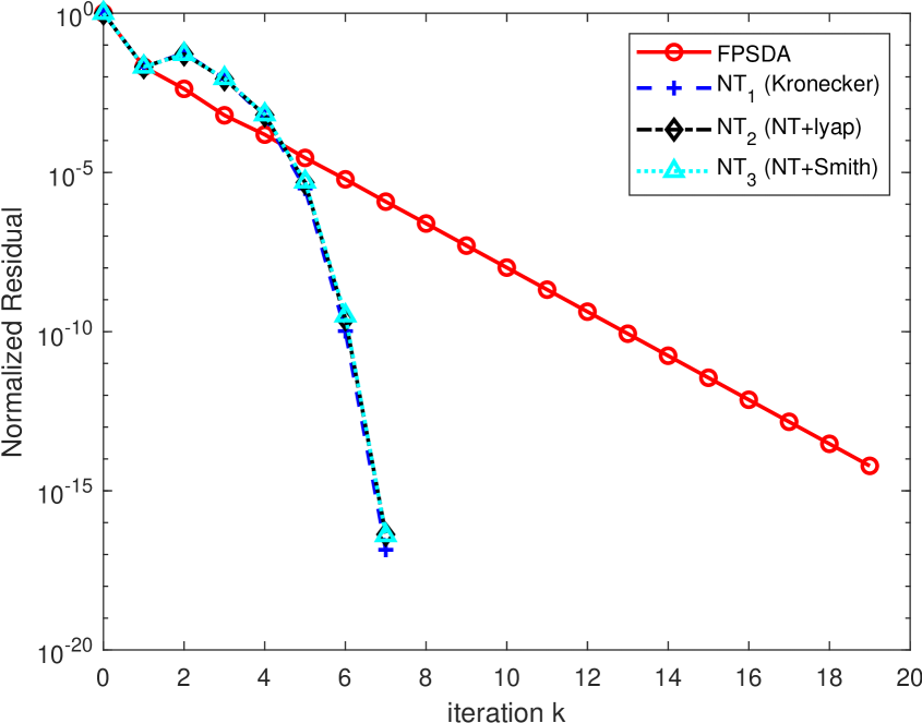
(a) Example 5.1

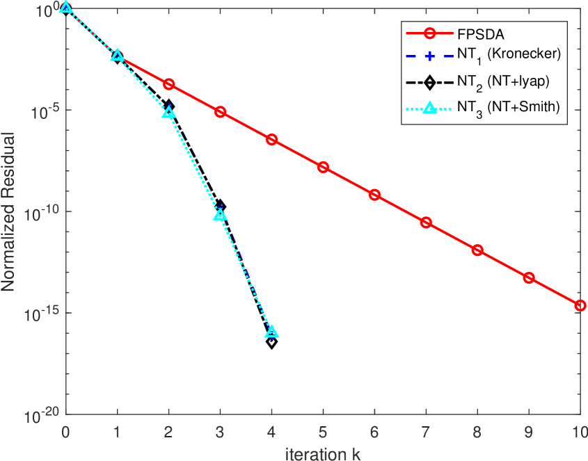
(b) Example 5.2 with $\varepsilon=0.01$

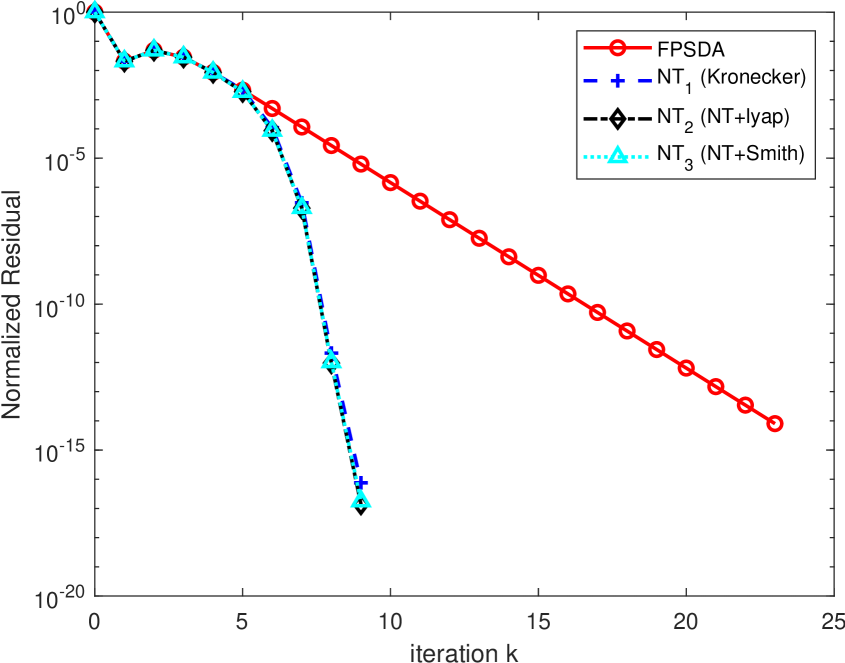
(c) Example 5.3

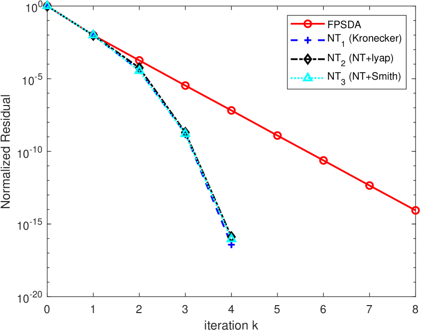
(d) Example 5.4 with $\varepsilon=5$

Figure 1: Iterative histories of fpsda, $\mbox{\sc nt}_{1}$ (via Kronecker’s reformulation of each Newton step equation), $\mbox{\sc nt}_{2}$ (via MATLAB’s lyap to iteratively solve Newton step equations), and $\mbox{\sc nt}_{3}$ (via Smith’s method to iteratively solve Newton step equations in an inner-outer fashion). The plotted histories of normalized residual by the variants of Newton’s method include the portion by fpsda for calculating an initial.

Example 5.1.

$A$, $B$, $Q$ and $R$ are taken from [2, Example 2.2]:

$$A=\begin{bmatrix}0.9512&0\\ 0&0.9048\end{bmatrix},\quad B=\begin{bmatrix}4.8770&4.8770\\ -1.1895&3.5690\end{bmatrix},\quad Q=\begin{bmatrix}0.005&0\\ 0&0.020\end{bmatrix},\quad R=\begin{bmatrix}\frac{1}{3}&0\\ 0&3\end{bmatrix},$$

while we set $L=0$, $r=3$ and

$$A_{0}^{1} =\begin{bmatrix}-0.1&0.1\\ -0.2&0.2\end{bmatrix},\quad A_{0}^{2}=\begin{bmatrix}1&-0.1\\ 0.5&0\end{bmatrix},\quad A_{0}^{3}=\begin{bmatrix}0&-0.2\\ 0.2&0.5\end{bmatrix},$$

$$B_{0}^{1} =\begin{bmatrix}0&-0.1\\ 0.1&0\end{bmatrix},\quad B_{0}^{2}=\begin{bmatrix}0.5&1\\ -0.1&0.2\end{bmatrix},\quad B_{0}^{3}=\begin{bmatrix}1&-1\\ -0.2&1\end{bmatrix}.$$

Example 5.2.

$A$, $B$, $Q$ and $R$ are taken from [16, Example 12]:

$$A=\varepsilon\begin{bmatrix}\frac{7}{3}&\frac{2}{3}&0\\ \frac{2}{3}&2&-\frac{2}{3}\\ 0&-\frac{2}{3}&\frac{5}{3}\end{bmatrix},\quad Q=\begin{bmatrix}(4\varepsilon+4+\varepsilon^{-1})/9&2(2\varepsilon-1-\varepsilon^{-1})/9&2(2-\varepsilon-\varepsilon^{-1})/9\\ 2(2\varepsilon-1-\varepsilon^{-1})/9&(1+4\varepsilon+4/\varepsilon)/9&2(-1-\varepsilon+2/\varepsilon)/9\\ 2(2-\varepsilon-\varepsilon^{-1})/9&2(-1-\varepsilon+2/\varepsilon)/9&(4+\varepsilon+4/\varepsilon)/9\end{bmatrix},$$

$$B=\frac{1}{\sqrt{\varepsilon}}I_{3},\quad R=I_{3},$$

where $\varepsilon=0.01$, while we set $L=0$, $r=1$ and

$$A_{0}^{1}=0.1\begin{bmatrix}0.1&-0.1&0.01\\ -0.2&0.1&-0.1\\ 0.05&-0.01&0.3\end{bmatrix},\quad\quad B_{0}^{1}=0.1\begin{bmatrix}0&0&0.2\\ 0.36&-0.6&0\\ 0&-0.95&-0.032\end{bmatrix}.$$

Example 5.3.

$A$, $B$, $Q$, $L$ and $R$ are taken from [39]:

$$A =\begin{bmatrix}0.9512&0\\ 0&0.9048\end{bmatrix},\quad B=\begin{bmatrix}4.8770&4.8770\\ -1.1895&3.5690\end{bmatrix},\quad Q=\begin{bmatrix}0.0028&-0.0013\\ -0.0013&0.0190\end{bmatrix},$$

$$R =\begin{bmatrix}1/3&0\\ 0&3\end{bmatrix},\quad L=0,$$

while $r=1$ and we modify $A_{0}^{1}$ and $B_{0}^{1}$ in [39] to

$$A_{0}^{1}=6.5\begin{bmatrix}0.1&0.2\\ 0.2&0.1\end{bmatrix},\quad B_{0}^{1}=6.5I_{2}.$$

Example 5.4.

$A$, $B$, $Q$ and $R$ are taken from [16, Example 11]:

$$A=\begin{bmatrix}3-\varepsilon&1\\ 4&2-\varepsilon\end{bmatrix},\quad B=\begin{bmatrix}1\\ 1\end{bmatrix},\quad Q=\begin{bmatrix}4\varepsilon-11&2\varepsilon-5\\ 2\varepsilon-5&2\varepsilon-2\end{bmatrix},\quad R=1,$$

where $\varepsilon=5$, while we set $L=0$, $r=1$ and

$$A_{0}^{1}=\begin{bmatrix}0.1&-0.1\\ -0.2&0.1\end{bmatrix},\quad B_{0}^{1}=\begin{bmatrix}0.1\\ 0\end{bmatrix}.$$

		$\mbox{\sc nt}_{1}$		$\mbox{\sc nt}_{2}$ (nt+lyap)		$\mbox{\sc nt}_{3}$ (nt+smith)		init. (fpsda)
	fpsda	#itn.	sol. err.	#itn.	sol. err.	#itn.	sol. err.	$\delta$ in (5.1)	#itn.
Example 5.1	(19,21)	6	$3.7{\scriptstyle(-14)}$	(6,23)	$3.7{\scriptstyle(-14)}$	(6,28,28)	$3.7{\scriptstyle(-14)}$	$0.5$	(1,2)
Example 5.2	(10,41)	3	$4.3{\scriptstyle(-15)}$	(3,8)	$4.4{\scriptstyle(-15)}$	(3,11,11)	$9.4{\scriptstyle(-15)}$	$0.5$	(1,5)
Example 5.3	(23,24)	5	$1.8{\scriptstyle(-13)}$	(5,30)	$1.9{\scriptstyle(-13)}$	(5,30,30)	$1.8{\scriptstyle(-13)}$	$10^{-2}$	(4,5)
Example 5.4	(8,8)	3	$2.0{\scriptstyle(-14)}$	(3,8)	$2.1{\scriptstyle(-14)}$	(3,10,10)	$2.0{\scriptstyle(-14)}$	$0.5$	(1,1)

Table 1: The numbers of outer and inner iterations and solution error against the one by fpsda, for solving scare (1.4). For an inner iteration, it is the total number, e.g., the total number of sda iterations for Example 5.1 by fpsda is 21. The iteration scheme of $\mbox{\sc nt}_{3}$ has 3 levels and hence each run of $\mbox{\sc nt}_{3}$ produces three numbers, e.g., for Example 5.1, $\mbox{\sc nt}_{3}$ consumes 6 Newton steps, a total of 28 Lypunov equations solved by Smith’s method and, altogether, a total of 28 Smith iterations are executed. The “sol. err.” is calculated as in (5.2) and listed in such a way that, e.g., $3.7{\scriptstyle(-14)}$ represents $3.7\cdot 10^{-14}$.

Figure 1 plots the iterative histories in terms of normalized residuals by fpsda and three variants of Newton’s methods. The initials for three variants of Newton’s method are calculated by fpsda to satisfy (5.1) with $\delta$ as specified in Table 1. It is noted that $\delta=10^{-2}$ is used for Example 5.3, much smaller than $\delta=0.5$ for the other three examples. It turns out that $\mbox{\sc nt}_{2}$ and $\mbox{\sc nt}_{3}$ diverge if with $\delta=0.5$ while $\mbox{\sc nt}_{1}$ still converges with $\delta=0.5$. This suggests that using the fixed-point type scheme for solving Newton step equations may need more accurate initial than the plain Newton’s method. Table 1 contains performance statistics of the numbers of outer iterations and the total numbers of inner iterations (in each level), and relative solution errors:

$$\frac{\|X_{\mbox{\sc nt}}-X_{\mbox{\sc fp}\mbox{\sc sda}}\|_{\operatorname{F}}}{\|X_{\mbox{\sc fp}\mbox{\sc sda}}\|_{\operatorname{F}}}$$ (5.2)

for the solutions $X_{\mbox{\sc nt}}$ by any of the three Newton variants against $X_{\mbox{\sc fp}\mbox{\sc sda}}$ by fpsda. The last column in Table 1 lists the numbers of outer and inner iterations by fpsda to calculate initials for Newton’s method to use.

From Figure 1 and Table 1, we made the following observations:

1. fpsda converges linearly while Newton’s method converges quadratically.

2. On average, there are only a few number of inner-most iterations per equation solving. In the case of fpsda, for all but Example 5.2, each freezed care takes about one sda iteration which means the approximation $X_{0}$ at line 3 of Algorithm B.1 suffices, while for Example 5.2, the average number of sda iterations per care is about $4$.

3. The stopping criterion at line 8 of Algorithm 4.1 can capture the quadratic convergence of Newton’s method at a cost of a few number of fixed-point iterations to solve each Newton step equation.

5.2 Real-World Problems

For the next four examples, $A_{0}^{1},\ldots,A_{0}^{r}$ and $B_{0}^{1},\ldots,B_{0}^{r}$ are constructed randomly with MATLAB’s wgn function for white Gaussian noises. Hence, they provides infinitely many testing problems. They are considerably harder than the previous four problems. In particular, Example 5.5 is too big ($n=199$) for $\mbox{\sc nt}_{1}$ in which Newton step equations are transformed to linear systems in the standard form and then solved by Gaussian elimination. More detailed observations will come later. The initials to the variants of Newton’s method are again calculated by fpsda such that (5.1) is satisfied with $\delta$ as specified in Table 2.

Example 5.5.

The coefficient matrices, $A$, $B$, $Q$, $R$, and $L$ are taken from a control model of position and velocity for a string of high-speed vehicles [1]:

$$A =\begin{bmatrix}E&F\\ &\ddots&\ddots\\ &&E&F\\ &&&E&-1\\ &&&&-1\end{bmatrix}\in\mathbb{R}^{(2m-1)\times(2m-1)}\quad\mbox{with}\quad E=\begin{bmatrix}-1&0\\ 1&0\end{bmatrix},\quad F=\begin{bmatrix}0&0\\ -1&0\end{bmatrix},$$

$$B =[b_{ij}]\in\mathbb{R}^{(2m-1)\times m}\quad\mbox{with}\quad b_{ij}=\begin{cases}1,&\mbox{ for }i=1,3,5,\ldots,2m-1,j=(i+1)/2,\\ 0,&\mbox{ otherwise},\end{cases}$$

$$Q =[q_{ij}]\in\mathbb{R}^{(2m-1)\times(2m-1)}\quad\mbox{with}\quad q_{ij}=\begin{cases}10,&\mbox{ for }i=2,4,6,\ldots,2m-1,\ j=i,\\ 0,&\mbox{ otherwise},\end{cases}$$

$$R =I_{m},\quad L=0_{(2m-1)\times m},$$

where $m$ is the number of vehicles, and hence $n=2m-1$, and $A_{0}^{1},\ldots,A_{0}^{5}$ and $B_{0}^{1},\ldots,B_{0}^{5}$ are multiplicative white noises constructed as

$$A_{0}^{i} =0.1\times i\times\frac{\|A\|_{\infty}}{\|\widehat{A}_{0}^{i}\|_{\infty}}\widehat{A}_{0}^{i}\text{ with }\widehat{A}_{0}^{i}=\mbox{{wgn}}(2m-1,2m-1,8\times i)\,\,\mbox{ for }i=1,\ldots,5,$$

$$B_{0}^{i} =0.15\times i\times\frac{\|B\|_{\infty}}{\|\widehat{B}_{0}^{i}\|_{\infty}}\widehat{B}_{0}^{i}\text{ with }\widehat{B}_{0}^{i}=\mbox{{wgn}}(2m-1,m,3\times i)\,\,\mbox{ for }i=1,\ldots,5.$$

In our test, $m=100$ yielding $n=199$, which turns out to be too big for $\mbox{\sc nt}_{1}$.

Example 5.6.

In [29, 32], a 3D missile/target interception engagement with impact angle guidance strategies is modeled by a state-dependent linear-structured dynamic system in the form of (1.1), where sdc matrices and white noise matrices are given by

$$A(\boldsymbol{x}) =\begin{bmatrix}0&1&0&0&0\\ 0&\frac{-2\dot{\varrho}}{\varrho}&0&\frac{-1}{2}\dot{\psi}\sin(2x_{1}+2\theta_{f})&\frac{g_{1}}{z_{a}}\\ 0&0&0&1&0\\ 0&2\dot{\psi}\tan(x_{1}+\theta_{f})&0&\frac{-2\dot{\varrho}}{\varrho}&\frac{g_{2}}{z_{a}}\\ 0&0&0&0&-\eta\end{bmatrix},\quad B(\boldsymbol{x})=\begin{bmatrix}0&0\\ \frac{-\cos\theta_{M}}{\varrho}&0\\ 0&0\\ \frac{\sin\theta_{M}\sin\psi_{M}}{\varrho\cos\theta}&\frac{-\cos\psi_{M}}{\varrho\cos\theta}\\ 0&0\end{bmatrix},$$

$$A_{0}^{i} =0.2\times i\times\frac{\|A\|_{\infty}}{\|\widehat{A}_{0}^{i}\|_{\infty}}\widehat{A}_{0}^{i}\ \text{ with }\ \widehat{A}_{0}^{i}=\mbox{{wgn}}(5,5,8\times i)\,\,\mbox{ for }i=1,\ldots,4,$$ (5.3a)

$$B_{0}^{i} =0.1\times i\times\frac{\|B\|_{\infty}}{\|\widehat{B}_{0}^{i}\|_{\infty}}\widehat{B}_{0}^{i}\ \text{ with }\ \widehat{B}_{0}^{i}=\mbox{{wgn}}(5,2,3\times i)\,\,\mbox{ for }i=1,\ldots,4,$$ (5.3b)

in which $\varrho$ measures the distance between the missile and the target, $\{\psi,\theta\}$ (respective to $\{\psi_{M},\theta_{M}\}$) are the azimuth and elevation angles (respective to missile) corresponding to the initial frame (respective to the line-of-sight (los) frame). Furthermore, the state vector $\boldsymbol{x}=[x_{1},x_{2},x_{3},x_{4},x_{5}]^{\operatorname{T}}$ satisfies

$$x_{1}=\theta-\theta_{f},\,\,x_{2}=\dot{x}_{1},\,\,x_{3}=\psi-\psi_{f},\,\,x_{4}=\dot{x}_{3}$$

with $\theta_{f}$ and $\psi_{f}$ being the prescribed final angles, $x_{5}$ is a slow varying stable auxiliary variable governed by $\dot{x}_{5}=-\eta x_{5}$ for some $\eta>0$, $g_{1}$ and $g_{2}$ are highly nonlinear functions of $\varrho$, $\theta$, $\psi$, $\theta_{f}$, $\psi_{f}$, $\theta_{T}$, $\psi_{T}$, $a_{T}^{z}$ and $a_{T}^{y}$ (see [32] for details), where $\{\psi_{T},\theta_{T}\}$ are the azimuth and elevation angles of the target to the los frame, $a_{T}^{z}$ and $a_{T}^{y}$ are the lateral accelerations for the target, and $(u_{1},u_{2})=(a_{M}^{z},a_{M}^{y})$ is the control vector for the maneuverability of missile.

As we explained in Section 1, the ssdre approach will repeatedly solve stochastic state-dependent care (1.3) at a number of fixed state $\boldsymbol{x}$. In this test, we will consider one such equation as an scare (1.4) with

$$A =\begin{bmatrix}0&1&0&0&0\\ 0&0.0696&0&-0.0307&-1.91\times 10^{-4}\\ 0&0&0&1&0\\ 0&0.123&0&0.0696&6.13\times 10^{-4}\\ 0&0&0&0&-0.1\end{bmatrix},\quad B=\begin{bmatrix}0&0\\ -9.13\times 10^{-5}&0\\ 0&0\\ 2.42\times 10^{-5}&-1.30\times 10^{-4}\\ 0&0\end{bmatrix},$$

$$Q ={\rm diag}(1000,1000,1000,1000,0),\quad R=I_{2},\quad L=0,\quad A_{0}^{i}\text{ and }B_{0}^{i}\text{ as in \eqref{eq6.1}.}$$

Example 5.7.

The F16 aircraft flight control system [15] can be described as a linear-structured dynamic system in the form of (1.1):

$$\dot{\boldsymbol{x}}\equiv\begin{bmatrix}\dot{u}\\ \dot{v}\\ \dot{w}\\ \dot{p}\\ \dot{q}\\ \dot{\varrho}\end{bmatrix}= \begin{bmatrix}(g\sin\theta)/u&0&0&0&-w&v\\ (-g\sin\phi\cos\theta)/u&0&0&w&0&-u\\ (-g\cos\phi\cos\theta)/u&0&0&-v&u&0\\ 0&0&0&c_{1}q/2&(c_{1}p+c_{2}\varrho)/2&c_{2}q/2\\ 0&0&0&c_{3}p+c_{4}\varrho/2&0&c_{4}p/2-c_{3}\varrho\\ 0&0&0&c_{5}q/2&(c_{5}p+c_{6}\varrho)/2&c_{6}q/2\end{bmatrix}\begin{bmatrix}u\\ v\\ w\\ p\\ q\\ \varrho\end{bmatrix}$$

$$+\begin{bmatrix}1/\mu&0&0&0\\ 0&0&0&0\\ 0&0&0&0\\ 0&c_{lp}&0&c_{\nu p}\\ c_{\mu q}Z_{TP}&0&c_{\mu q}&0\\ 0&c_{l\varrho}&0&c_{\nu\varrho}\end{bmatrix}\begin{bmatrix}F_{T}\\ L\\ M\\ N\end{bmatrix}\equiv A(\boldsymbol{x})\boldsymbol{x}+B(\boldsymbol{x})\boldsymbol{u},$$

where $g$ is the gravity force, $\mu$ is the aircraft mass, $(u,v,w)$ and $(p,q,\varrho)$ are the aircraft velocity and angular velocity vectors, respectively, for roll $\phi$, pitch $\theta$ and yaw $\psi$ angles, parameters $c$ with various subscripts are the suitable combinations of coefficients of the aircraft inertial matrix, the control vector $\boldsymbol{u}=[F_{T},L,M,N]^{\operatorname{T}}$ consists of the thrust $F_{T}$ and the aircraft moment vector $[L,M,N]^{\operatorname{T}}$, and $Z_{TP}$ is the position of the thrust point.

In this test, we consider scare (1.4), from solving the optimization problem (1.2) at a fixed state by the ssdre approach, with coefficient matrices:

$$A =\begin{bmatrix}3.958\times 10^{-5}&0&0&0&-5.866&-6.985\\ 2.116\times 10^{-4}&0&0&5.866&0&-84.66\\ -0.1158&0&0&6.985&84.66&0\\ 0&0&0&1.791\times 10^{-4}&4.303\times 10^{-3}&-5.006\times 10^{-3}\\ 0&0&0&-5.329\times 10^{-3}&0&-4.259\times 10^{-2}\\ 0&0&0&-4.769\times 10^{-3}&3.253\times 10^{-2}&-1.791\times 10^{-4}\end{bmatrix},$$

$$B =\begin{bmatrix}1.076\times 10^{-4}&0&0&0\\ 0&0&0&0\\ 0&0&0&0\\ 0&7.780\times 10^{-5}&0&7.780\times 10^{-5}\\ 3.964\times 10^{-6}&0&1.321\times 10^{-5}&0\\ 0&1.211\times 10^{-6}&0&1.171\times 10^{-5}\end{bmatrix},$$

$$Q =5000I_{6},\quad R=2\times 10^{-4}I_{4},\quad L=0,$$

$$A_{0}^{i} =0.012\times i\times\frac{\|A\|_{\infty}}{\|\widehat{A}_{0}^{i}\|_{\infty}}\widehat{A}_{0}^{i}\ \text{ with }\ \widehat{A}_{0}^{i}=\mbox{{wgn}}(6,6,100\times i)\,\,\mbox{ for }i=1,2,3,$$

$$B_{0}^{i} =0.012\times i\times\frac{\|B\|_{\infty}}{\|\widehat{B}_{0}^{i}\|_{\infty}}\widehat{B}_{0}^{i}\ \text{ with }\ \widehat{B}_{0}^{i}=\mbox{{wgn}}(6,4,40\times i)\,\,\mbox{ for }i=1,2,3.$$

(a) Example 5.5 with $m=100$

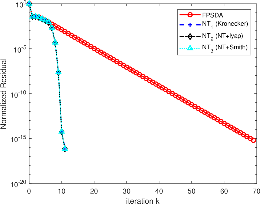
(b) Example 5.6

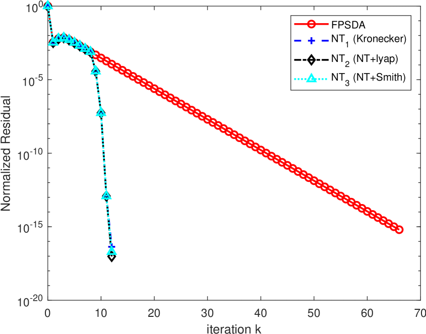
(c) Example 5.7

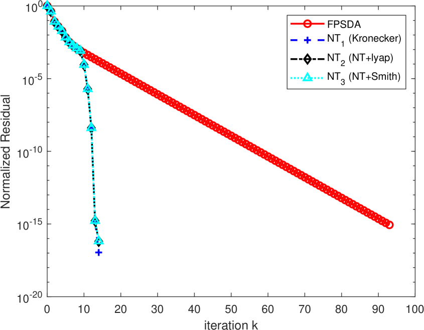
(d) Example 5.8

Figure 2: Iterative histories of fpsda, $\mbox{\sc nt}_{1}$ (via Kronecker’s reformulation of each Newton step equation), $\mbox{\sc nt}_{2}$ (via MATLAB’s lyap to iteratively solve Newton step equations), and $\mbox{\sc nt}_{3}$ (via Smith’s method to iteratively solve Newton step equations in an outer-inner fashion). The plotted histories of normalized residual by the variants of Newton’s method include the portion by fpsda for calculating an initial.

Example 5.8.

The sdre optimal control design for quadrotors for enhancing robustness against unmodeled disturbances [14] can be described as in (1.1) and (1.2a) with $\boldsymbol{x}=[u,v,w,p,q,\varrho,\phi,\theta,z_{a}]^{\operatorname{T}}$,

$$A(\boldsymbol{x}) =\begin{bmatrix}0&\frac{\varrho}{2}&-\frac{q}{2}&0&-\frac{w}{2}&\frac{v}{2}&0&-\frac{g(\sin\theta)}{\theta}&0\\ -\frac{\varrho}{2}&0&\frac{p}{2}&\frac{w}{2}&0&-\frac{u}{2}&\frac{g(1+\cos\theta)\sin\phi}{2\phi}&-\frac{g(1-\cos\theta)\sin\phi}{2\theta}&0\\ \frac{q}{2}&-\frac{p}{2}&0&-\frac{v}{2}&\frac{u}{2}&0&-\frac{2g}{\phi}\sin^{2}(\frac{\phi}{2})\cos^{2}(\frac{\theta}{2})&-\frac{2g}{\theta}\sin^{2}(\frac{\theta}{2})\cos^{2}(\frac{\phi}{2})&\frac{g}{z_{a}}\\ 0&0&0&0&\frac{c_{1}\varrho}{2}&\frac{c_{1}q}{2}&0&0&0\\ 0&0&0&\frac{c_{2}\varrho}{2}&0&\frac{c_{2}p}{2}&0&0&0\\ 0&0&0&\frac{c_{3}q}{2}&\frac{c_{3}p}{2}&0&0&0&0\\ 0&0&0&1&\frac{\sin\phi\tan\theta}{3}&\frac{\tan\theta(1+\cos\phi)}{3}&\frac{\alpha_{1}}{3\phi}&\frac{\alpha_{2}}{3\theta}&0\\ 0&0&0&0&\frac{1+\cos\phi}{2}&-\frac{\sin\phi}{2}&-\frac{\alpha_{3}}{2\phi}&0&0\\ 0&0&0&0&0&0&0&0&-\eta\end{bmatrix},$$

$$B =\begin{bmatrix}0&0&-1/\mu&0&0&0&0&0&0\\ 0&0&0&{1}/{{\cal I}_{x}}&0&0&0&0&0\\ 0&0&0&0&{1}/{{\cal I}_{y}}&0&0&0&0\\ 0&0&0&0&0&{1}/{{\cal I}_{z}}&0&0&0\end{bmatrix}^{\operatorname{T}},$$

$$Q =\mbox{\rm diag}(2000,2000,3000,10,10,100,0,0,0),\ R=I_{4},\ L=0,$$

$$A_{0}^{i} =0.025\times i\times\frac{\|A\|_{\infty}}{\|\widehat{A}_{0}^{i}\|_{\infty}}\widehat{A}_{0}^{i}\ \text{ with }\ \widehat{A}_{0}^{i}=\mbox{{wgn}}(9,9,10\times i)\,\,\mbox{ for }i=1,2,3,$$

$$B_{0}^{i} =0.01\times i\times\frac{\|B\|_{\infty}}{\|\widehat{B}_{0}^{i}\|_{\infty}}\widehat{B}_{0}^{i}\ \text{ with }\ \widehat{B}_{0}^{i}=\mbox{{wgn}}(9,4,4\times i)\,\,\mbox{ for }i=1,2,3,$$

where $g$ is the gravity force, $\mu$ is the quadrotor mass, $(u,v,w)$ and $(p,q,\varrho)$ are the velocity and the angular velocity on the body-fixed frame, respectively, for roll $\phi$, pitch $\theta$ and yaw $\psi$ angles,

$$\alpha_{1} =q\tan\theta\sin\phi-\varrho\tan\theta+\varrho\tan\theta\cos\phi,$$

$$\alpha_{2} =q\tan\theta\sin\phi+\varrho\tan\theta\cos\phi,$$

$$\alpha_{3} =q(1-\cos\phi)+\varrho\sin\phi,$$

$z_{a}$ is a slow varying stable auxiliary variable governed by $\dot{z}_{a}=-\eta z_{a}$, $\eta>0$, $c_{1}=({\cal I}_{y}-{\cal I}_{z})/{\cal I}_{x}$, $c_{2}=({\cal I}_{z}-{\cal I}_{x})/{\cal I}_{y}$, $c_{3}=({\cal I}_{x}-{\cal I}_{y})/{\cal I}_{z}$, and ${\cal I}_{x}$, ${\cal I}_{y}$, and ${\cal I}_{z}$ are inertia parameters.

With $\mu=1$, ${\cal I}_{x}={\cal I}_{y}=0.01466$, and ${\cal I}_{z}=0.02848$, an instance of $A(\boldsymbol{x})$ is

$$A =\begin{bmatrix}0&-8.208\mbox{e-}4&-1.047\mbox{e-}2&0&-1.234\mbox{e-}4&1.178&0&-9.8000&0\\ 8.208\mbox{e-}4&0&-1.603\mbox{e-}3&1.234\mbox{e-}4&0&2.203\mbox{e-}2&9.800&-5.436\mbox{e-}4&0\\ 1.047\mbox{e-}2&1.603\mbox{e-}3&0&-1.178&-2.203\mbox{e-}2&0&0&0&9.820\mbox{e-}1\\ 0&0&0&0&7.738\mbox{e-}4&-9.871\mbox{e-}3&0&0&0\\ 0&0&0&-7.738\mbox{e-}4&0&-1.511\mbox{e-}3&0&0&0\\ 0&0&0&0&0&0&0&0&0\\ 0&0&0&1.000&1.386\mbox{e-}8&2.499\mbox{e-}4&2.617\mbox{e-}6&-5.464\mbox{e-}4&0\\ 0&0&0&0&1.000&0&-9.650\mbox{e-}3&0&0\\ 0&0&0&0&0&0&0&0&-0.100\end{bmatrix},$$

yielding an scare (1.4) to solve.

		$\mbox{\sc nt}_{1}$		$\mbox{\sc nt}_{2}$ (nt+lyap)		$\mbox{\sc nt}_{3}$ (nt+smith)		init. (fpsda)
	fpsda	#itn.	sol. err.	#itn.	sol. err.	#itn.	sol. err.	$\delta$ in (5.1)	#itn.
Example 5.5	(18,71)			(6,25)	$2.8{\scriptstyle(-13)}$	(6,36,36)	$2.8{\scriptstyle(-13)}$	$10^{-2}$	(1,3)
Example 5.6	(69,144)	5	$9.5{\scriptstyle(-15)}$	(5,287)	$9.8{\scriptstyle(-15)}$	(5,231,231)	$9.7{\scriptstyle(-15)}$	$10^{-2}$	(6,18)
Example 5.7	(66,137)	4	$3.3{\scriptstyle(-14)}$	(4,96)	$3.5{\scriptstyle(-14)}$	(4,99,99)	$3.5{\scriptstyle(-14)}$	$10^{-3}$	(8,21)
Example 5.8	(93,553)	5	$5.8{\scriptstyle(-13)}$	(5,174)	$6.3{\scriptstyle(-13)}$	(5,203,203)	$6.4{\scriptstyle(-13)}$	$10^{-3}$	(9,49)

Table 2: The numbers of outer and inner iterations and solution error against the one by fpsda, for solving scare (1.4). For Example 5.5, each Newton’s step has a linear system of $199^{2}$-by-$199^{2}$ in the standard form to solve and that is too big for most personal PC. That is why there is no result reported for $\mbox{\sc nt}_{1}$.

As before, Figure 2 plots the iterative histories in terms of normalized residuals by fpsda and three variants of Newton’s methods on these four examples, while Table 2 contains performance statistics of the number of outer iterations and the total number of inner iterations (in each level), and relative solution errors measured as in (5.2).

We note again that these examples have random components and hence each call will generate a different scare. From Figure 2 and Table 2 and from numerous runs on these (random) examples, we observed the following:

1. With $n=2m-1=199$ in Example 5.5, $\mbox{\sc nt}_{1}$ will have to face $199^{2}$-by-$199^{2}$ linear systems in the standard form converted from Newton step equations via Kronecker’s product. That is too big for everyday PC/laptops such as ours. For that reason, no result is reported on Example 5.5 by $\mbox{\sc nt}_{1}$. On the other hand, all other methods work perfectly well on the example.

2. fpsda converges linearly and the convergence can be slow, as indicated by the large numbers of outer and inner iterations, especially for the last three examples. Newton’s method converges quadratically and consumes very few (outer) numbers of iterations, helped by relatively accurate initials by fpsda. But note that both $\mbox{\sc nt}_{2}$ and $\mbox{\sc nt}_{3}$ requires large number of inner iterations.

3. For the last three examples, each Newton step equation takes from 24 to 57 fixed-point iterations, i.e., the number of times $\widehat{\Pi}_{k}(\cdot)$ in (4.2a) is frozen, but for Example 5.5, the number is between 4 and 6. On the other hand, on average, the number of Smith’s iteration step is 1.

4. On average, the number of sda iterations per care in fpsda is between 2 and 6.

5. There are nontrivial chances that Examples 5.7 and 5.8 may not have psd stabilizing solutions as fpsda fail to converge when it is run many times (hence with different random noises). Likely not every random realization of them satisfies Assumptions 1.1 and 1.2 in Section 1.

6. It is reasonable to say that these later four problems are harder than the previous four problems, judging from reading the performance statistics in Tables 1 and 2.

6 Conclusions

The state-dependent Riccati equation approach, although suboptimal, is a systematic way to study nonlinear optimal control problems. The basic idea is to formulate a nonlinear optimal control problem into one with the same linear structure as in the mature linear optimal control theory. Practical applications have demonstrated its successes. In the approach for systems with stochastic noises, the so-called stochastic continuous-time algebraic Riccati equation (scare)

$$A^{\operatorname{T}}X+XA+Q+\Pi_{11}(X)-[XB+L+\Pi_{12}(X)][R+\Pi_{22}(X)]^{-1}[XB+L+\Pi_{12}(X)]^{\operatorname{T}}=0,$$

frequently arises and has to be solved repeatedly, and ideally in real time, e.g., for the 3D missile/target engagement, the F16 aircraft flight control, and the quadrotor optimal control, to name a few. Newton’s method had been called for the task previously, but existing research focuses more on the theoretic aspect than numerical one, e.g., there is no practical way to pick an initial guess to enure convergence.

In this paper, we propose a robust and efficient inner-outer iterative scheme to solve the scare efficiently and accurately. It is based on the fixed-point technique and the structure-preserving doubling algorithm (sda). The basic idea is to first freeze $X$ in the linear matrix-valued functions $\Pi_{ij}(\cdot)$ at the current approximate solution and then apply sda to the resulting continuous algebraic Riccati equation (care). It is proved, among others, that the method is monotonically convergent to the desired stabilizing solution. The new method is called fpsda for short.

We revisit Newton’s method to investigate how to calculate each Newton iterative step efficiently and how to select sufficiently accurate initial guesses so that Newton’s method can become practical. These are important issues that have not received much attention previously.

Both methods, ours and Newton’s method with our implementation ideas, are applied to a collection of scare, both artificial and real-world ones, to validate our claims and intuitive ideas.

Appendix A Fixed-point iteration

The basic idea of creating a fixed-point iteration (fp) is to first transform scare (1.4) equivalently to an equation of the form

$$X=\mathscr{F}(X)$$ (A.1)

which immediately leads to an iterative scheme:

given $$X_{0} X_{k+1}=\mathscr{F}(X_{k}) k=0,1,2,\ldots$$, iterate for (A.2)

until convergence, if it is convergent. Guo and Liang [22] propose one such $\mathscr{F}(\cdot)$ and proved that the associated fp converges.

Guo and Liang [22] construct their $\mathscr{F}(\cdot)$ as follow. Factorize $Q-LR^{-1}L^{\operatorname{T}}=\widehat{C}^{\operatorname{T}}\widehat{C}$. In theory, this factorization exists because $Q-LR^{-1}L^{\operatorname{T}}\succeq 0$. Always $\widehat{C}$ has $n$ columns, but its number of rows is not unique, except no fewer than the rank of $Q-LR^{-1}L^{\operatorname{T}}\succeq 0$. Numerically, any such a factor $\widehat{C}$ works. Let

$$\widehat{A}=A-BR^{-1}L^{\operatorname{T}},\quad\widehat{B}=BR^{-1/2},$$

and let $P\in\mathbb{R}^{nr\times nr}$ and $\widehat{P}\in\mathbb{R}^{n(r+1)\times n(r+1)}$ be the permutation matrices such that

$$P^{\operatorname{T}}(X\otimes I_{r})P =I_{r}\otimes X,$$

$$\operatorname{diag}(X,X\otimes I_{r}) =\widehat{P}^{\operatorname{T}}(X\otimes I_{r+1})\widehat{P},$$

and

$$\mathscr{A}=P\left(\begin{bmatrix}A_{0}^{1}\\ \vdots\\ A_{0}^{r}\end{bmatrix}-\begin{bmatrix}B_{0}^{1}\\ \vdots\\ B_{0}^{r}\end{bmatrix}R^{-1}L^{\operatorname{T}}\right)\in\mathbb{R}^{nr\times n},\quad\mathscr{B}=P\begin{bmatrix}B_{0}^{1}\\ \vdots\\ B_{0}^{r}\end{bmatrix}R^{-/12}\in\mathbb{R}^{nr\times m}.$$

Given $\gamma<0$ so that $\widehat{A}_{\gamma}:=\widehat{A}+\gamma I_{n}$ is nonsingular. scare (1.4) can be transformed into

$$X=\mathscr{F}(X):=E_{\gamma}^{\operatorname{T}}(X\otimes I_{r+1})\left[I_{n(r+1)}+G_{\gamma}(X\otimes I_{r+1})\right]^{-1}E_{\gamma}+H_{\gamma},$$ (A.3)

where, with $Z_{\gamma}=\widehat{C}\widehat{A}_{\gamma}^{-1}\widehat{B}$,

$$E_{\gamma} =\widehat{P}\begin{bmatrix}\widehat{A}_{\gamma}-2\gamma I_{n}+\widehat{B}Z_{\gamma}^{\operatorname{T}}\widehat{C}\\ \sqrt{-2\gamma}(\mathscr{A}+\mathscr{B}Z_{\gamma}^{\operatorname{T}}\widehat{C})\end{bmatrix}(I_{n}+\widehat{A}_{\gamma}^{-1}\widehat{B}Z_{\gamma}^{\operatorname{T}}\widehat{C})^{-1}\widehat{A}_{\gamma}^{-1}\in\mathbb{R}^{n(r+1)\times n},$$ (A.4a)

$$H_{\gamma} =-2\gamma\widehat{A}_{\gamma}^{-\operatorname{T}}\widehat{C}^{\operatorname{T}}(I_{\ell}+Z_{\gamma}Z_{\gamma}^{\operatorname{T}})^{-1}\widehat{C}\widehat{A}_{\gamma}^{-1}\in\mathbb{R}^{n\times n},$$ (A.4b)

$$G_{\gamma} =\widehat{P}\begin{bmatrix}\sqrt{-2\gamma}\widehat{A}_{\gamma}^{-1}\widehat{B}\\ \mathscr{A}\widehat{A}_{\gamma}^{-1}\widehat{B}-\mathscr{B}\end{bmatrix}(I_{m}+Z_{\gamma}^{\operatorname{T}}Z_{\gamma})^{-1}\begin{bmatrix}\sqrt{-2\gamma}\widehat{A}_{\gamma}^{-1}\widehat{B}\\ \mathscr{A}\widehat{A}_{\gamma}^{-1}\widehat{B}-\mathscr{B}\end{bmatrix}^{\operatorname{T}}\widehat{P}^{\operatorname{T}}\in\mathbb{R}^{n(r+1)\times n(r+1)}.$$ (A.4c)

Guo and Liang [22] propose to start their fp with $X_{0}=0$ in (A.2) and prove its convergence for any $\gamma<0$ such that $\widehat{A}_{\gamma}$ is invertible. Conceivably, the rate of convergence is dependent of the parameter $\gamma$, but it is not clear, even intuitively, how to choose $\gamma$ for fast convergence.

Another problematic issue is that $\mathscr{F}(\cdot)$ in (A.3) involves the inverse of $I_{n(r+1)}+G_{\gamma}(X_{k}\otimes I_{r+1})\in\mathbb{R}^{n(r+1)\times n(r+1)}$, which can be a drag, unless $n(r+1)$ is modest (under $1,000$ or smaller). In what follows, inspired by the construction of the first standard form (SF1) in [24], we will propose another $\mathscr{F}$ for (A.1) in what follows. We begin with pretending $A_{\operatorname{c}}(\cdot)$, $G_{\operatorname{c}}(\cdot)$, and $H_{\operatorname{c}}(\cdot)$ in (2.2) are constant matrices and apply the construction in [24, section 5.3] to matrix pencil

$$\begin{bmatrix}A_{\operatorname{c}}(X)&-G_{\operatorname{c}}(X)\\ -H_{\operatorname{c}}(X)&-\big{[}A_{\operatorname{c}}(X)\big{]}^{\operatorname{T}}\end{bmatrix}-\lambda I_{2n}.$$ (A.5)

Given $\gamma\in\mathbb{R}$ such that $A_{\operatorname{c},\gamma}(X):=A_{\operatorname{c}}(X)+\gamma I_{n}$ is invertible, symbolically following the procedure there, we end up with its SF1 as

$$\begin{bmatrix}E_{\operatorname{c}}(X)&0\\ -X_{\operatorname{c}}(X)&I_{n}\end{bmatrix}-\lambda\begin{bmatrix}I&-Y_{\operatorname{c}}(X)\\ 0&\big{[}E_{\operatorname{c}}(X)\big{]}^{\operatorname{T}}\end{bmatrix},$$ (A.6)

where

$$S(X) =-\big{[}A_{\operatorname{c},\gamma}(X)\big{]}^{\operatorname{T}}-H_{\operatorname{c}}(X)\,[A_{\operatorname{c},\gamma}(X)]^{-1}G_{\operatorname{c}}(X),$$ (A.7a)

$$E_{\operatorname{c}}(X) =I_{n}+2\gamma[S(X)]^{-1},$$ (A.7b)

$$X_{\operatorname{c}}(X) =2\gamma[S(X)]^{-1}H_{\operatorname{c}}(X)[A_{\operatorname{c},\gamma}(X)]^{-1},$$ (A.7c)

$$Y_{\operatorname{c}}(X) =-2\gamma[A_{\operatorname{c},\gamma}(X)]^{-1}G_{\operatorname{c}}(X)[S(X)]^{-1}.$$ (A.7d)

Finally, the primal equation associated with (A.6) is given by [24, p.27]

$$X=\mathscr{F}(X):=X_{\operatorname{c}}(X)+E_{\operatorname{c}}(X)\,X[I_{n}-Y_{\operatorname{c}}(X)\,X]^{-1}E_{\operatorname{c}}(X)$$ (A.8)

which is equivalent to (1.6) and, hence, scare (1.4). We make a couple of comments regarding the fp based on (A.8) as follows.

1. $X_{k+1}=\mathscr{F}(X_{k})$ with (A.8) is in fact the second approximation by sda  (Algorithm B.1) applied to (2.2) with $A_{\operatorname{c}}(\cdot)$, $G_{\operatorname{c}}(\cdot)$, and $H_{\operatorname{c}}(\cdot)$ freezed at $X_{k}$. This connection leads to an intuitive way to construct an effective $\gamma$ that varies from one iterative step to another by examining the eigenvalues in $\mathbb{C}_{-}$ of the matrix pencil (A.5) with frozen $A_{\operatorname{c}}(\cdot)$, $G_{\operatorname{c}}(\cdot)$, and $H_{\operatorname{c}}(\cdot)$, as we discussed in Appendix B below.

2. Each fp iterative step based on (A.8) involves three inverses of $n$-by-$n$ matrices. This compares favorably with fp based on (A.3) for large $n$. Here is why. Suppose that the computational complexity of inverting an $n$-by-$n$ matrix is $cn^{3}$ where $c$ is some constant. Then the matrix inversion costs per fp iterative step is $3cn^{3}$ for (A.8) and $(r+1)^{3}cn^{3}$ for (A.3). The cost ratio is $(r+1)^{3}/3$ which is $8/3=2.67$ for $r=1$ and grows rather fast as $r$ increases.

Appendix B Structure-Preserving Doubling Algorithm for care

We review the structure-preserving doubling algorithm (sda) for care, which will be tailored to serve as the workhorse for our Algorithm 3.1. For more detail, the reader is referred to [24, chapter 5]. care has a couple of equivalent forms, but the one we will be considering is as follows:

$$A^{\operatorname{T}}X+XA-XGX+H=0,$$ (B.1)

where $A$, $G^{\operatorname{T}}=G$, and $H^{\operatorname{T}}=H$ are in $\mathbb{R}^{n\times n}$.

Theorem B.1 (e.g., [41, p.330]).

Suppose that $G\succeq 0$ and $H\succeq 0$. If $(A,G)$ is stabilizable and $(H,A)$ is detectable, then care (B.1) has a unique positive semidefinite (psd) solution $X_{*}$, and, moreover, the solution is stabilizing, i.e., $\operatorname{eig}(A-GX_{*})\subset\mathbb{C}_{-}$, the left half of the complex plane.

This is essentially Corollary 13.8 of [41, p.330] which is stated for $G=BB^{\operatorname{T}}$ and $H=C^{\operatorname{T}}C$ along with the condition that $(A,B)$ is stabilizable and $(C,A)$ is detectable. Theorem B.1 is equivalent to the corollary because $G\succeq 0$ and $H\succeq 0$ imply that $G=BB^{\operatorname{T}}$ and $H=C^{\operatorname{T}}C$ for some $B\in\mathbb{R}^{n\times m}$ and $C\in\mathbb{R}^{\ell\times n}$, and because $(A,G)$ is stabilizable if and only if $(A,B)$ is stabilizable, and $(H,A)$ is detectable if and only if $(C,A)$ is detectable.

Algorithm B.1 sda for care  (B.1)

0:  $A,\,G,\,H\in\mathbb{R}^{n\times n}$ with $G^{\operatorname{T}}=G,\,H^{\operatorname{T}}=H$;

0:  $X_{*}$, the last $X_{i}$, as the computed solution to (B.1).  

1:  pick an appropriate $\gamma<0$;

2:  compute $A_{+\gamma}=A+\gamma I$, $A_{-\gamma}=A-\gamma I$, $S=-A_{+\gamma}^{\operatorname{T}}-HA_{+\gamma}^{-1}G$;

3:  compute $E_{0}=I+2\gamma S^{-\operatorname{T}}$ and then

$$X_{0} =2\gamma S^{-1}HA_{+\gamma}^{-1},$$

$$Y_{0} =A_{+\gamma}^{-1}G-A_{+\gamma}^{-1}GS^{-1}(-HA_{+\gamma}^{-1}G-A_{-\gamma}^{\operatorname{T}});$$

4:  for $k=0,1,\ldots,$ until convergence do

5:     compute $E_{k+1}=E_{k}(I_{m}-Y_{k}X_{k})^{-1}E_{k}$ and then

$$X_{k+1} =X_{k}+E_{k}^{\operatorname{T}}X_{k}(I_{n}-Y_{k}X_{k})^{-1}E_{k},$$

$$Y_{k+1} =Y_{k}+E_{k}(I_{n}-Y_{k}X_{k})^{-1}Y_{k}E_{k}^{\operatorname{T}};$$

6:  end for

7:  return  last $X_{k}$ as the computed solution at convergence.

The unique psd solution $X_{*}\succeq 0$ mentioned in Theorem B.1 can be efficiently calculated by sda [24, 31], as outlined in Algorithm B.1, for modest $n$ (up to a couple of thousands so that matrix inversions can be efficiently implemented). Under the conditions of Theorem B.1, Algorithm B.1 runs without any breakdown for any $\gamma<0$ such that $A_{+\gamma}:=A+\gamma I$ is invertible, i.e., all inverses at line 5 exist, and the sequence $\{X_{k}\}_{k=0}^{\infty}$ is monotonically increasing and convergent:

$$0\preceq X_{0}\preceq X_{1}\preceq\cdots\preceq X_{k}\to X_{*},$$ (B.2)

and the convergence is quadratic. sda does not need an initial to begin with and $X_{0}$ at line 3 can be considered as the first approximation by sda. Also $\{Y_{k}\}_{k=0}^{\infty}$ converges, too, but to the stabilizing solution of the dual care of (B.1) [24, chapter 5].

sda starts by selecting a shift $\gamma<0$. In theory, any $\gamma<0$ will work, but some $\gamma$ is better than others for speedy convergence of sda. For the fastest asymptotical rate of convergence, the optimal $\gamma$ is given by [25, 24]

$$\gamma:=\arg\min_{\lambda\in\operatorname{eig}(A-GX_{*})}\left|\frac{\lambda-\gamma}{\lambda+\gamma}\right|.$$

Finding this optimal $\gamma$ can be time consuming or outright impractical, and hence is not recommended, but usually a suboptimal one is good enough due to the quadratic convergence of sda. Here is an idea from [25] for small $n$ (under ten or even up to a few hundreds) as in most of our later numerical examples:

1. calculate the $n$ eigenvalues in $\mathbb{C}_{-}$ of

   $$\begin{bmatrix}A&-G\\ -H&-A^{\operatorname{T}}\end{bmatrix};$$

2. encircle these $n$ eigenvalues by a rectangle $[a,b]\times[-c,c]$ where $a\leq b<0$, and set

   $$\gamma=\begin{cases}-\sqrt{b^{2}+c^{2}},&\mbox{if $c^{2}\geq b(a-b)/2$},\\ -\sqrt{ab-c^{2}},&\mbox{if $c^{2}<b(a-b)/2$}.\end{cases}$$ (B.3)

For more guidelines and discussions on how to pick a suboptimal $\gamma$, the reader is referred to [25]. Also required on $\gamma$ in Algorithm B.1 is that $A_{+\gamma}$ is well-conditioned for its inversion.

When $G=0$, (B.1) reduces to a Lyapunov’s equation

$$A^{\operatorname{T}}X+XA+H=0.$$ (B.4)

It is well-known that (B.4) always has a unique solution $X_{*}$ if $\operatorname{eig}(A)\subset\mathbb{C}_{-}$, and moreover $X_{*}\succeq 0$ if also $H\succeq 0$. Note now the requirements on stabilizability and detectability as in Theorem B.1 are no longer needed. As a special case of (B.1), Lyapunov’s equation (B.4) can be solved by sda, too, and the resulting method is much simpler because now $Y_{k}=0$ for all $k$. Specifically, the sda iteration for (B.4) becomes

$$E_{0}=I-2\gamma A_{+\gamma}^{-1},\,\,X_{0}=-2\gamma A_{+\gamma}^{-\operatorname{T}}HA_{+\gamma}^{-1},\,\,\mbox{and}$$ (B.5a)

$$E_{k+1}=E_{k}^{2},\,\,X_{k+1}=X_{k}+E_{k}^{\operatorname{T}}X_{k}E_{k}\,\,\,\mbox{for $k\geq 0$}.$$ (B.5b)

It coincides with Smith’s method, which broadly is for solving Sylvester’s equation [37, 38].

It remains to address how to stop the for-loop in Algorithm B.1 properly. We refer the reader to [24, 40] for more discussions in general. In the case of solving scare (1.4) in Section 3, Algorithm B.1 is used as an inner iteration to calculate an update to the current approximation of the stabilizing solution to (1.4) so that the next approximation is more accurate after the update. For that purpose, there is no need to solve any intermediate care fully accurately in the working precision. In fact, ideally, the update should be calculated with just enough accuracy so that any more accuracy in the update will not help. Also, in Section 3, $H=\mathscr{R}(\widetilde{X}_{k})$ at the $k$th iteration. In view of this discussion, in our use of Algorithm B.1, we stop the for-loop if

$$\|A^{\operatorname{T}}X_{k}+X_{k}A-X_{k}GX_{k}+H\|_{\operatorname{F}}\leq\tau\cdot\|H\|_{\operatorname{F}},$$ (B.6)

where $0<\tau<1$ is a preselected error-reducing factor. Unfortunately, optimal $\tau$ is problem-dependent. We tested $\tau=1/2,\,1/4,\,1/8,\,1/10$ and found $\tau=1/8$ provide a good balance to achieve small numbers of inner and outer iterations. We point out two advantages of (B.6) over any of the general purposed criteria discussed in [24, 40]:

1. (B.6) is cheaper and friendlier to use than general stopping criteria discussed in [24, 40] because it does not require calculating $\|A\|_{\operatorname{F}},\,\|G\|_{\operatorname{F}},\,\|H\|_{\operatorname{F}}$, and $\|X_{k}\|_{2}$, needed for calculating the normalized residual of the care at the point.

2. (B.6) usually stops the for-loop much sooner because of fairly large $\tau$.

In the case of Smith’s method (B.4) as an inner iteration, it is terminated if

$$\|A^{\operatorname{T}}X_{k}+X_{k}A+H\|_{\operatorname{F}}\leq\tau\cdot\|H\|_{\operatorname{F}}.$$ (B.7)

Appendix C A modified Newton’s method

Guo [21] considered a special case of scare (1.4): $L=0$ and $B_{0}^{i}=0$ for $i=1,\ldots,r$. For the special case, each Newton step solves a linear matrix equation having exactly the same form as (4.2a). Guo proposed a modified Newton method: simply freeze the term $\widehat{\Pi}_{k}(\cdot)$ at $X_{k}$ and solve

$$\widehat{A}_{k}^{\operatorname{T}}X_{k+1}+X_{k+1}\widehat{A}_{k}+\widehat{\Pi}_{k}(X_{k})+M_{k}=0$$ (C.1)

instead. It does get around the difficulty of solving generalized Lyapunov’s equations in Newton’s method, but loses the generic quadratic convergence of the method.

This idea of creating a modified Newton method straightforwardly carries over to our more general scare (1.4), too. For the ease of reference, we outline the modified Newton’s method as in Algorithm C.1. Its implementation is mostly straightforward, except that when Lyapunov’s equation (C.1) in $X_{k+1}$ is solved iteratively, by, e.g., Smith’s method, there are a couple of comments worthy mentioning for efficient numerical performance:

1. (C.1) should be solved for an update $Z$ to $X_{k}$ to yield $X=X_{k}+Z$:

   $$A_{k}^{\operatorname{T}}Z+Z\widehat{A}_{k}+\underbrace{(A_{k}^{\operatorname{T}}X_{k}+X_{k}\widehat{A}_{k}+C_{k})}_{=:\widetilde{C}_{k}}=0,$$

   which is solved iteratively, starting from $Z_{0}=0$, where $C_{k}=\widehat{\Pi}_{k}(X_{k})+M_{k}$.

2. We may use

   $$\|\widehat{A}_{k}^{\operatorname{T}}Z_{i}+Z_{i}\widehat{A}_{k}+\widetilde{C}_{k}\|_{\operatorname{F}}\leq\tau\cdot\|\widetilde{C}_{k}\|_{\operatorname{F}},$$

   knowing that the modified Newton’s method is likely linearly convergent, where ideally $\tau$ is just small enough so that, as an approximation to the desired solution of scare (1.4), $X_{k}+Z_{i}$ is about as accurate as if $Z_{i}$ solves the updating equation exactly, but practical $\tau$ around $1/8$ usually works well.

Algorithm C.1 Modified Newton’s method (m​nt) for solving scare (1.4)

0:  $A,Q\in\mathbb{R}^{n\times n}$, $B,L\in\mathbb{R}^{n\times m}$, $R=R^{\operatorname{T}}\in\mathbb{R}^{m\times m}$, $A_{0}^{i}\in\mathbb{R}^{n\times n}$, $B_{0}^{i}\in\mathbb{R}^{n\times m}$ for $i=1,\ldots,r$, initial $X_{0}^{\operatorname{T}}=X_{0}$, and a tolerance $\varepsilon$.

0:  $X_{*}$, the last $X_{k}$, as the computed solution to (1.4).  

1:  $k=0$;

2:  while $\operatorname{NRes}(X_{k})>\varepsilon$ do

3:     $S_{k}=X_{k}B+L+\Pi_{12}(X_{k})$, $R_{k}=\Pi_{22}(X_{k})+R$;

4:     $\widehat{A}_{k}=A-BR_{k}^{-1}S_{k}^{\operatorname{T}}$, $P_{k}=\begin{bmatrix}I\\ -R_{k}^{-1}S_{k}^{\operatorname{T}}\end{bmatrix}$, $M_{k}=P_{k}^{\operatorname{T}}\begin{bmatrix}Q&L\\ L^{\operatorname{T}}&R\end{bmatrix}P_{k}$;

5:     $C_{k}=P_{k}^{\operatorname{T}}\Pi(X_{k})P_{k}+M_{k}$;

6:     solve $\widehat{A}_{k}^{\operatorname{T}}X+X\widehat{A}_{k}+C_{k}=0$ for $X$, e.g., by Smith’s method, a special case of sda (see discussions in Appendix B after Algorithm B.1) or by the Bartels-Stewart method [7], and set $X_{k+1}$ to be the computed solution;

7:     Set $k=k+1$;

8:  end while

9:  return  $X_{*}=X_{k}$.

C.1 Convergence Analysis

Let $\{X_{k}\}_{k=0}^{\infty}$ be generated by m​nt (Algorithm C.1). A sufficient condition for Algorithm C.1 to be able to generate the entire sequence is $\operatorname{eig}(\widehat{A}_{k})\subset\mathbb{C}_{-}$ for all $k$.

For the special case: $L=0$ and $B_{0}^{i}=0$ for $i=1,\ldots,r$, Guo established the following convergence theorem, assuming that $X_{k+1}$ is the exact solution of (C.1).

Theorem C.1 ([21]).

Consider scare (1.4) with $L=0$ and $B_{0}^{i}=0$ for $i=1,\ldots,r$, and let $X_{*}\succeq 0$ be a solution. Suppose Algorithm C.1 starts with initial $X_{0}$ that satisfies $X_{0}\succeq X_{*}$, $A_{0}-G_{0}X_{0}$ is stable and $\mathscr{R}(X_{0})\preceq 0$. Then

1. $\operatorname{eig}(\widehat{A}_{k})\subset\mathbb{C}_{-}$ and $\mathscr{R}(X_{k})\preceq 0$ for all $k\geq 0$,

2. $X_{0}\succeq X_{1}\succeq\cdots\succeq X_{k}\succeq X_{*}$ for all $k\geq 0$, and

3. $\lim_{k\to\infty}X_{k}=X_{*+}$, a maximal solution of scare (1.4).

Note that, in Theorem C.1, $X_{*+}$ is a maximal solution of scare (1.4). Going forward, we will assume (3.4) as in our convergence analysis for fpsda in Section 3.2. In particular, Assumptions 1.1 and 1.2 are assumed and hence scare (1.4) has a unique psd  solution $X_{*}$, which is stabilizing. Hence, $X_{*+}=X_{*}$ in Theorem C.1 for the case.

In what follows, we will consider the more general case without requiring $L=0$ or $B_{0}^{i}=0$ for $i=1,\ldots,r$. But we need to assume that $\{X_{k}\}_{k=0}^{\infty}$ by Algorithm C.1 exists and $X_{k}\succeq 0$ for all $k$. Again it is assumed that (C.1) is solved exactly. Under these assumptions, we will show that $\{X_{k}\}_{k=0}^{\infty}$ is monotonically convergent.

By (2.1a), (4.2d), and (4.2e), and noticing $S_{k}=X_{k}B+L_{k}$, we have

$$\widehat{\Pi}_{k}(X_{k})+M_{k} =\begin{bmatrix}I\\ -R_{k}^{-1}S_{k}^{\operatorname{T}}\end{bmatrix}^{\operatorname{T}}\begin{bmatrix}Q_{k}&L_{k}\\ L_{k}^{\operatorname{T}}&R_{k}\end{bmatrix}\begin{bmatrix}I\\ -R_{k}^{-1}S_{k}^{\operatorname{T}}\end{bmatrix}$$

$$=Q_{k}-L_{k}R_{k}^{-1}S_{k}^{\operatorname{T}}-S_{k}R_{k}^{-1}L_{k}^{\operatorname{T}}+S_{k}R_{k}^{-1}S_{k}^{\operatorname{T}}$$

$$=H_{k}+X_{k}BR_{k}^{-1}B^{\operatorname{T}}X_{k},$$ (C.2)

where $H_{k}=H_{\operatorname{c}}(X_{k})=Q_{k}-L_{k}R_{k}^{-1}L_{k}^{\operatorname{T}}$. Hence the modified Newton’s iteration equation (C.1) is transformed into

$$A_{k}^{\operatorname{T}}X_{k+1}+X_{k+1}A_{k}-X_{k+1}G_{k}X_{k+1}+H_{k}+(X_{k+1}-X_{k})G_{k}(X_{k+1}-X_{k})=0.$$ (C.3)

Lemma C.1.

Assume (3.4) and suppose $X_{k}\succeq 0$. Then $A_{k}-G_{k}X_{k}$ is stable if and only if $X_{k+1}\succeq 0$.

Proof.

It follows from Lemma 2.2 that $(H_{k},A_{k})$ is detectable, where $H_{k}=A_{\operatorname{c}}(X_{k})$ and $A_{k}=A_{\operatorname{c}}(X_{k})$ as before. Factorize $H_{k}=C_{k}^{\operatorname{T}}C_{k}$. By (4.2c) and (C.2), we have

$$(A_{k}-G_{k}X_{k})^{\operatorname{T}}X_{k+1}+X_{k+1}(A_{k}-G_{k}X_{k})=-(H_{k}+X_{k}G_{k}X_{k}).$$

Recall $\widehat{A}_{k}=A_{k}-G_{k}X_{k}$. If $\widehat{A}_{k}$ is stable, then $X_{k+1}\succeq 0$ by Lemma 3.1.

Suppose $X_{k+1}\succeq 0$. We now prove $\operatorname{eig}(A_{k}-G_{k}X_{k})\subset\mathbb{C}-$. Assume, to the contrary, that $A_{k}-G_{k}X_{k}$ is not stable. Then there exist $\mathbb{C}^{n}\ni\boldsymbol{y}\neq 0$ and $\Re(\lambda)\geq 0$ such that $(A_{k}-G_{k}X_{k})\boldsymbol{y}=\lambda\boldsymbol{y}$, which implies

$$0\leq 2\Re(\lambda)\boldsymbol{y}^{\operatorname{H}}X_{k+1}\boldsymbol{y}=-(\boldsymbol{y}^{\operatorname{H}}H_{k}\boldsymbol{y}+\boldsymbol{y}^{\operatorname{H}}X_{k}G_{k}X_{k}\boldsymbol{y}).$$

Since $H_{k},G_{k}\succeq 0$, we conclude that $H_{k}\boldsymbol{y}=0$ and $G_{k}X_{k}\boldsymbol{y}=0$. Consequently,

$$\lambda\boldsymbol{y}=(A_{k}-G_{k}X_{k})\boldsymbol{y}=A_{k}\boldsymbol{y},\quad\boldsymbol{y}\neq 0,\quad\Re(\lambda)\geq 0,\quad\mbox{ and }\quad H_{k}\boldsymbol{y}=0,$$

contradicting that the detectability of $(H_{k},A_{k})$ is detectable. ∎

Our first convergence result is that $\{X_{k}\}_{k=0}^{\infty}$ by Algorithm C.1 is monotonically decreasing.

Theorem C.2.

Assume (3.4). Suppose that initial $X_{0}$ satisfies

$$X_{0}\succeq X_{*},\,\,\operatorname{eig}(A_{0}-G_{0}X_{0})\in\mathbb{C}_{-},\,\,\mathscr{R}(X_{0})\preceq 0.$$ (C.4)

If $X_{k}\succeq 0$ for all $k$, then we have

1. $X_{0}\succeq X_{1}\succeq\cdots\succeq X_{k}\succeq X_{*}$, $\mathscr{R}(X_{k})\preceq 0$ for $k\geq 0$;

2. $\lim_{k\rightarrow\infty}X_{k}=X_{*}$.

Proof.

By Lemma C.1 and by the assumption that $X_{k}\succeq 0$ for all $k$, we conclude that $A_{k}-G_{k}X_{k}$ is stable for all $k\geq 0$. First we show, by induction, that for $k\geq 0$

$$X_{k}\succeq X_{k+1},\ \ X_{k}\succeq X_{*}\text{ and }\mathscr{R}(X_{k})\preceq 0,$$ (C.5)

and, as a result, item (a) holds. For $k=0$, we already have $X_{0}\succeq X_{*}$ and $\mathscr{R}(X_{0})\preceq 0$ by assumption. It remains to show that $X_{0}\succeq X_{1}$. To this end, by (C.2), we have

$$(A_{0}-G_{0}X_{0})^{\operatorname{T}}(X_{1}-X_{0})+(X_{1}-X_{0})(A_{0}-G_{0}X_{0})=-\mathscr{R}(X_{0})\succeq 0.$$

Since $A_{0}-G_{0}X_{0}$ is stable, by Lemma 3.1 we conclude that $X_{0}\succeq X_{1}$. Suppose now that (C.5) is true for $k=\ell$. We will prove it for $k=\ell+1$. Let $k=\ell$ in (C.3) to get

$$(A_{\ell}-G_{\ell}X_{\ell})^{\operatorname{T}} (X_{*}-X_{\ell+1})+(X_{*}-X_{\ell+1})(A_{\ell}-G_{\ell}X_{\ell})$$

$$=\begin{bmatrix}X_{*}\\ -I\end{bmatrix}^{\operatorname{T}}\Omega(X_{\ell})\begin{bmatrix}X_{*}\\ -I\end{bmatrix}+(X_{*}-X_{\ell})G_{\ell}(X_{*}-X_{\ell})$$

$$\succeq\begin{bmatrix}X_{*}\\ -I\end{bmatrix}^{\operatorname{T}}\Omega(X_{*})\begin{bmatrix}X_{*}\\ -I\end{bmatrix}+(X_{*}-X_{\ell})G_{\ell}(X_{*}-X_{\ell})$$

$$=(X_{*}-X_{\ell})G_{\ell}(X_{*}-X_{\ell})$$

$$\succeq 0,$$

where we have used $X_{\ell}\succeq X_{*}$ which implies $\Omega(X_{\ell})\succeq\Omega(X_{*})$ by Lemma 2.3, and Lemma 2.4 and $X_{*}$ is a solution to scare (1.4). Therefore, $X_{\ell+1}\succeq X_{*}$ by Lemma 3.1. Next, we show that $X_{\ell+1}\succeq X_{\ell+2}$ and $\mathscr{R}(X_{\ell+1})\preceq 0$. By the induction hypothesis, $X_{\ell}\succeq X_{\ell+1}$ which implies $\Omega(X_{\ell})\succeq\Omega(X_{\ell+1})$ by Lemma 2.3, and hence we have

$$\mathscr{R}(X_{\ell+1}) =A_{\ell+1}^{\operatorname{T}}X_{\ell+1}+X_{\ell+1}A_{\ell+1}-X_{\ell+1}G_{\ell+1}X_{\ell+1}+H_{\ell+1}$$

$$=\begin{bmatrix}X_{\ell+1}\\ -I\end{bmatrix}^{\operatorname{T}}\Omega(X_{\ell+1})\begin{bmatrix}X_{\ell+1}\\ -I\end{bmatrix}$$

$$\preceq\begin{bmatrix}X_{\ell+1}\\ -I\end{bmatrix}^{\operatorname{T}}\Omega(X_{\ell})\begin{bmatrix}X_{\ell+1}\\ -I\end{bmatrix}$$

$$=-(X_{\ell+1}-X_{\ell})G_{\ell}(X_{\ell+1}-X_{\ell})\qquad(\mbox{by \eqref{eq:mNT4SCARE-step'} for $k=\ell$})$$

$$\preceq 0.$$

Finally, letting $k=\ell+1$ in (C.3) yields

$$(A_{\ell+1}-G_{\ell+1}X_{\ell+1})^{\operatorname{T}} (X_{\ell+2}-X_{\ell+1})+(X_{\ell+2}-X_{\ell+1})(A_{\ell+1}-G_{\ell+1}X_{\ell+1})$$

$$=\begin{bmatrix}X_{\ell+2}\\ -I\end{bmatrix}^{\operatorname{T}}\Omega(X_{\ell+1})\begin{bmatrix}X_{\ell+2}\\ -I\end{bmatrix}-\begin{bmatrix}X_{\ell+1}\\ -I\end{bmatrix}^{\operatorname{T}}\Omega(X_{\ell+1})\begin{bmatrix}X_{\ell+1}\\ -I\end{bmatrix}$$

$$\qquad\qquad+(X_{\ell+2}-X_{\ell+1})G_{\ell+1}(X_{\ell+2}-X_{\ell+1})$$

$$=-\begin{bmatrix}X_{\ell+1}\\ -I\end{bmatrix}^{\operatorname{T}}\Omega(X_{\ell+1})\begin{bmatrix}X_{\ell+1}\\ -I\end{bmatrix}$$

$$=-\mathscr{R}(X_{\ell+1})\succeq 0,$$

yielding $X_{\ell+1}\succeq X_{\ell+2}$ by Lemma 3.1. The induction process is completed.

Since the psd solution $X_{*}$ of scare (1.4) is unique, item (b) is a corollary of item (a). ∎

The first condition in (C.4) requires that the initial $X_{0}$ is above the unique psd solution $X_{*}$ of scare (1.4). Next, we consider the case to start at $X_{0}$ that is below $X_{*}$.

Given $W\in\mathbb{H}^{n\times n}$, define linear operator $\mathscr{F}_{W}$ in $\mathbb{H}^{n\times n}$ as

$$\mathscr{F}_{W}(Z):=\begin{bmatrix}-I_{n}\\ R_{\operatorname{c}}(W)^{-1}\big{[}L_{\operatorname{c}}(W)+WB\big{]}^{\operatorname{T}}\end{bmatrix}^{\operatorname{T}}\,\Pi(Z)\,\begin{bmatrix}-I\\ R_{\operatorname{c}}(W)^{-1}\big{[}L_{\operatorname{c}}(W)+WB\big{]}^{\operatorname{T}}\end{bmatrix}.$$ (C.6)

Not that if $Z\succeq 0$, then $\mathscr{F}_{W}(Z)\succeq 0$ because $\Pi(Z)\succeq 0$ for any $Z\succeq 0$. But we will need something stronger than this in what follows.

Assumption C.1.

There exists $\alpha>0$ such that $\mathscr{F}_{X_{*}}(Z)\succeq\alpha\,Z\,\,\mbox{for all $Z\succeq 0$}.$

Given $W\in\mathbb{H}^{n\times n}$, define matrix-valued function $F_{W}(Y)$ in $\mathbb{H}^{n\times n}$ as

$$F_{W}(Y):=\begin{bmatrix}Y\\ -I_{n}\end{bmatrix}^{\operatorname{T}}\Big{[}\Omega(Y)-\Omega(W)\Big{]}\begin{bmatrix}Y\\ -I_{n}\end{bmatrix}\quad\mbox{for $Y\in\mathbb{H}^{n\times n}$}.$$ (C.7)

Lemma C.2.

Suppose that Assumption C.1 holds. Given $X_{0}\preceq X_{*}$, if $\|X_{*}-X_{0}\|_{2}$ is sufficiently small, then we have

$$F_{W}(Y)-(Y-W)BR^{-1}B^{\operatorname{T}}(Y-W)\succeq 0\quad\mbox{for $X_{0}\preceq W\preceq Y\preceq X_{*}$}.$$ (C.8)

Proof.

The right-hand side of (C.6) is continuous with respect to $W\in\mathbb{H}^{n\times n}$. Hence Assumption C.1 ensures that for sufficiently small $\|W-X_{*}\|_{2}$, we have $\mathscr{F}_{W}(Z)\succeq(2\alpha/3)\,Z$ for all $Z\succeq 0$.

It can be seen that $\mathscr{F}_{W}(Z)$ is the Frèchet derivative of $F_{W}$ at $Y=W$ along $Z$. The first-order expansion of $F_{W}(Y)$ at $Y=W$ is

$$F_{W}(Y) =\left.F_{W}^{\prime}(Y)\right|_{Y=W}[Y-W]+O(\|Y-W\|_{2}^{2})$$

$$=\mathscr{F}_{W}(Y-W)+O(\|Y-W\|_{2}^{2}).$$

If $\|X_{*}-X_{0}\|_{2}$ is sufficiently small, so is $\|W-Y\|_{2}$. Hence for sufficiently small $\|X_{*}-X_{0}\|_{2}$, we have

$$F_{W}(Y) \succeq(2\alpha/3)\,(Y-W)+O(\|Y-W\|_{2}^{2})$$

$$\succeq(\alpha/3)\,(Y-W),$$

Therefore, again for sufficiently small $\|X_{*}-X_{0}\|_{2}$, we have

$$F_{W}(Y)-(Y-W)BR^{-1}B^{\operatorname{T}}(Y-W) \succeq(\alpha/3)\,(Y-W)-\|BR^{-1}B^{\operatorname{T}}\|_{2}(Y-W)^{2}$$

$$=(Y-W)^{1/2}\Big{[}(\alpha/3)I_{n}-\|BR^{-1}B^{\operatorname{T}}\|_{2}(Y-W)\Big{]}(Y-W)^{1/2}$$

$$\succeq 0,$$

provided $(\alpha/3)I_{n}\succeq\|BR^{-1}B^{\operatorname{T}}\|_{2}(Y-W)$ which can be guaranteed by making $\|X_{*}-X_{0}\|_{2}$ sufficiently small. ∎

The purpose of having Lemma C.2 is to justify the requirement in the next theorem on the sufficient closeness of the initial $X_{0}$ to $X_{*}$ such that (C.8) holds for any $X_{0}\preceq W\preceq Y\preceq X_{*}$. One of the assumption in both Theorems C.3 and C.2 is that $X_{k}\succeq 0$ for all $k$, which is upsetting. Ideally, we should look for other reasonable assumptions that can ensure $X_{k}\succeq 0$ for all $k$, but we are unable to do so now.

Theorem C.3.

Assume (3.4), and suppose that Assumption C.1 holds and that initial $X_{0}$ satisfies

$$0\preceq X_{0}\preceq X_{*},\,\,\mbox{\eqref{eq:suff-close} holds for any $X_{0}\preceq Y\preceq W\preceq X_{*}$, and}\,\,\mathscr{R}(X_{0})\succeq 0.$$

If $X_{k}\succeq 0$ for all $k$, then we have

1. $0\preceq X_{0}\preceq X_{1}\preceq\cdots\preceq X_{k}\preceq X_{*}$ and $\mathscr{R}(X_{k})\succeq 0$ for all $k\geq 0$;

2. $\lim_{k\rightarrow\infty}X_{k}=X_{*}$.

Proof.

We prove item (a) by induction. For $k=0$, we already have $X_{0}\preceq X_{*}$ and $\mathscr{R}(X_{0})\succeq 0$. By (C.2), we have

$$(A_{0}-G_{0}X_{0})^{\operatorname{T}}(X_{1}-X_{0})+(X_{1}-X_{0})(A_{0}-G_{0}X_{0})=-\mathscr{R}(X_{0})\preceq 0.$$

Since $A_{0}-G_{0}X_{0}$ is stable, by Lemma 3.1, we obtain that $X_{0}\preceq X_{1}$. Suppose now that item (a) is true for $k=\ell\geq 0$. We will prove it for $k=\ell+1$. It can be verified by (C.3) for $k=\ell$ that

$$(A_{\ell}-G_{\ell}X_{\ell})^{\operatorname{T}}(X_{*}-X_{\ell+1}) +(X_{*}-X_{\ell+1})(A_{\ell}-G_{\ell}X_{\ell})$$

$$=\begin{bmatrix}X_{*}\\ -I\end{bmatrix}^{\operatorname{T}}\Omega(X_{\ell})\begin{bmatrix}X_{*}\\ -I\end{bmatrix}+(X_{*}-X_{\ell})G_{\ell}(X_{*}-X_{\ell})$$

$$=-\begin{bmatrix}X_{*}\\ -I\end{bmatrix}^{\operatorname{T}}\Big{[}\Omega(X_{*})-\Omega(X_{\ell})\Big{]}\begin{bmatrix}X_{*}\\ -I\end{bmatrix}+(X_{*}-X_{\ell})G_{\ell}(X_{*}-X_{\ell})$$

$$=-F_{X_{\ell}}(X_{*})+(X_{*}-X_{\ell})G_{\ell}(X_{*}-X_{\ell})$$

$$\preceq 0,$$

where we have used (2.21) and that $X_{*}$ is a solution to scare (1.4) for the second equality, and Lemma C.2 and $0\preceq X_{\ell}\preceq X_{*}$ for the last inequality. Therefore, $X_{\ell+1}\preceq X_{*}$ by Lemma 3.1. Next, we show that $X_{\ell+1}\preceq X_{\ell+2}$ and $\mathscr{R}(X_{\ell+1})\succeq 0$. Since

$$\begin{bmatrix}X_{\ell+1}\\ -I\end{bmatrix}^{\operatorname{T}}\Omega(X_{\ell})\begin{bmatrix}X_{\ell+1}\\ -I\end{bmatrix}+(X_{\ell+1}-X_{\ell})G_{\ell}(X_{\ell+1}-X_{\ell})=0,$$

we have

$$\mathscr{R}(X_{\ell+1}) =\begin{bmatrix}X_{\ell+1}\\ -I\end{bmatrix}^{\operatorname{T}}\Omega(X_{\ell+1})\begin{bmatrix}X_{\ell+1}\\ -I\end{bmatrix}$$

$$=\begin{bmatrix}X_{\ell+1}\\ -I\end{bmatrix}^{\operatorname{T}}\Big{[}\Omega(X_{\ell+1})-\Omega(X_{\ell})\Big{]}\begin{bmatrix}X_{\ell+1}\\ -I\end{bmatrix}-(X_{\ell+1}-X_{\ell})G_{\ell}(X_{\ell+1}-X_{\ell})$$

$$=F_{X_{\ell}}(X_{\ell+1})-(X_{\ell+1}-X_{\ell})G_{\ell}(X_{\ell+1}-X_{\ell})$$

$$\succeq 0,$$

where we have used $X_{0}\preceq X_{\ell}\preceq X_{\ell+1}\preceq X_{*}$ and Lemma C.2. Finally,

$$(A_{\ell+1}-G_{\ell+1}X_{\ell+1})^{\operatorname{T}} (X_{\ell+2}-X_{\ell+1})+(X_{\ell+2}-X_{\ell+1})(A_{\ell+1}-G_{\ell+1}X_{\ell+1})$$

$$=-\begin{bmatrix}X_{\ell+1}\\ -I\end{bmatrix}^{\operatorname{T}}\Omega(X_{\ell+1})\begin{bmatrix}X_{\ell+1}\\ -I\end{bmatrix}$$

$$=-\mathscr{R}(X_{\ell+1})\preceq 0.$$

Hence, $X_{\ell+1}\preceq X_{\ell+2}$ by Lemma 3.1. The induction process is completed.

Since the psd solution $X_{*}$ of scare (1.4) is unique, item (b) is a corollary of item (a). ∎

References

- [1] J. Abels and P. Benner. CAREX - a collection of benchmark examples for continuous-time algebraic Riccati equations. SLICOT Working Note 1999-16 (Version 2.0), December 1999. Available online at slicot.org/working-notes/.
- [2] J. Abels and P. Benner. DAREX – a collection of benchmark examples for discrete-time algebraic Riccati equations. SLICOT Working Note 1999-14 (Version 2.0), December 1999. Available online at slicot.org/working-notes/.
- [3] A. Alla, D. Kalise, and V. Simoncini. State-dependent Riccati equation feedback stabilization for nonlinear PDEs. Adv. in Comput. Math., 49(1):9 (32 pages), 2023.
- [4] M. Asgari and H. N. Foghahayee. State dependent Riccati equation (SDRE) controller design for moving obstacle avoidance in mobile robot. SN Applied Sciences, 2(11):1928 (29 pages), 2020.
- [5] R. Babazadeh and R. Selmic. Distance-based multi-agent formation control with energy constraints using SDRE. IEEE Trans. Aerosp. Electron. Syst., 56(1):41–56, 2020.
- [6] H. T. Banks, B. M. Lewis, and H. T. Tran. Nonlinear feedback controllers and compensators: a state-dependent Riccati equation approach. Comput. Optim. Appl., 37(2):177–218, 2007.
- [7] R. H. Bartels and G. W. Stewart. Algorithm 432: The solution of the matrix equation . Commun. ACM, 8:820–826, 1972.
- [8] P. Benner and T. Breiten. Low rank methods for a class of generalized Lyapunov equations and related issues. Numer. Math., 124(3):441–470, 2013.
- [9] P. Benner and J. Heiland. Exponential stability and stabilization of extended linearizations via continuous updates of Riccati-based feedback. Int. J. Robust Nonlinear Control, 28(4):1218–1232, 2018.
- [10] P. Benner, R.-C. Li, and N. Truhar. On ADI method for Sylvester equations. J. Comput. Appl. Math., 233(4):1035–1045, 2009.
- [11] T. Breiten and E. Ringh. Residual-based iterations for the generalized Lyapunov equation. BIT Numer. Math., 59(4):823–852, 2019.
- [12] T. Çimen. State-dependent Riccati equation (SDRE) control: A survey. IFAC Proceedings Volumes, 41(2):3761–3775, 2008. 17th IFAC World Congress.
- [13] T. Çimen. Survey of state-dependent Riccati equation in nonlinear optimal feedback control synthesis. J. Guid. Control Dyn., 35(4):1025–1047, 2012.
- [14] S.-W. Cheng and H.-A. Hung. Robust state-feedback control of quadrotor. International Automatic Control Conference, 2022.
- [15] M. Chodnicki, P. Pietruszewski, M. Weso ̵lowski, and S. Stȩpień. Finite-time SDRE control of F16 aircraft dynamics. Arch. Control Sci., 32:557–576, 2022.
- [16] E. K.-W. Chu, H.-Y. Fan, and W.-W. Lin. A structure-preserving doubling algorithm for continuous-time algebraic Riccati equations. Linear Algebra Appl., 396:55–80, 2005.
- [17] E. K.-W. Chu, T. Li, W.-W. Lin, and C.-Y. Weng. A modified Newton’s method for rational Riccati equations arising in stochastic control. In 2011 International Conference on Communications, Computing and Control Applications (CCCA), pages 1–6, 2011.
- [18] T. Damm. Rational Matrix Equations in Stochastic Control. Springer, Berlin, 2004.
- [19] T. Damm and D. Hinrichsen. Newton’s method for a rational matrix equation occuring in stochastic control. Linear Algebra Appl., 332-334:81–109, 2001.
- [20] V. Dragan, T. Morozan, and A.-M. Stoica. Mathematical Methods in Robust Control of Linear Stochastic Systems. Springer-Verlag, 2013.
- [21] C.-H. Guo. Iterative solution of a matrix Riccati equation arising in stochastic control. In Linear Operators and Matrices, pages 209–221. Birkhäuser Basel, 2002.
- [22] Z.-C. Guo and X. Liang. Stochastic algebraic Riccati equations are almost as easy as deterministic ones theoretically. SIAM J. Matrix Anal. Appl., 44(4):1749–1770, 2023.
- [23] Y. Hao and V. Simoncini. The sherman–morrison–woodbury formula for generalized linear matrix equations and applications. Numer. Linear Algebra Appl., 28(5):e2384, 2021.
- [24] T.-M. Huang, R.-C. Li, and W.-W. Lin. Structure-Preserving Doubling Algorithms for Nonlinear Matrix Equations. Society for Industrial and Applied Mathematics, Philadelphia, PA, 2018.
- [25] T.-M. Huang, R.-C. Li, W.-W. Lin, and L.-Z. Lu. Optimal parameters for doubling algorithms. J. Math. Study, 50(4):339–357, 2017.
- [26] I. G. Ivanov. Iterations for solving a rational Riccati equation arising in stochastic control. Comput. Math. Appl., 53:977–988, 2007.
- [27] P. Lancaster and L. Rodman. Algebraic Riccati Equations. Oxford Science Publications. Oxford University Press, 1995.
- [28] L.-G. Lin, Y.-W. Liang, and L.-J. Cheng. Control for a class of second-order systems via a state-dependent Riccati equation approach. SIAM J. Control Optim., 56(1):1–18, 2018.
- [29] L.-G. Lin, R.-S. Wu, P.-K. Huang, M. Xin, C.-T. Wu, and W.-W. Lin. Fast SDDRE-based maneuvering-target interception at prespecified orientation. pages 1–8, 2023.
- [30] L.-G. Lin and M. Xin. Alternative SDRE scheme for planar systems. IEEE Trans. Circuits Syst. II-Express Briefs, 66(6):998–1002, 2019.
- [31] W.-W. Lin and S.-F. Xu. Convergence analysis of structure-preserving doubling algorithms for Riccati-type matrix equations. SIAM J. Matrix Anal. Appl., 28(1):26–39, 2006.
- [32] R. V. Nanavati, S. R. Kumar, and A. Maity. Spatial nonlinear guidance strategies for target interception at pre-specified orientation. Aerosp. Sci. Technol., 114:106735, 2021.
- [33] S. R. Nekoo. Tutorial and review on the state-dependent Riccati equation. 8(2):109–166, 2019.
- [34] J. D. Pearson. Approximation methods in optimal control I. sub-optimal control. J. Elec. Control, 13(5):453–469, 1962.
- [35] S. D. Shank, V. Simoncini, and D. B. Szyld. Efficient low-rank solution of generalized Lyapunov equations. Numer. Math., 134(2):327–342, 2016.
- [36] V. Simoncini. A new iterative method for solving large-scale Lyapunov matrix equations. SIAM J. Sci. Comput., 29(3):1268–1288, 2007.
- [37] R. A. Smith. Matrix equation . SIAM J. Appl. Math., 16(1):198–201, 1968.
- [38] W.-G. Wang, W.-C. Wang, and R.-C. Li. Alternating-directional doubling algorithm for -matrix algebraic Riccati equations. SIAM J. Matrix Anal. Appl., 33:170–194, 2012.
- [39] P. C.-Y. Weng and F. K.-H. Phoa. Perturbation analysis and condition numbers of rational Riccati equations. Ann. Math. Sci. Appl., 6:25–49, 2021.
- [40] J.-G. Xue, S.-F. Xu, and R.-C. Li. Accurate solutions of M-matrix algebraic Riccati equations. Numer. Math., 120:671–700, 2012.
- [41] K. Zhou, J. C. Doyle, and K. Glover. Robust and Optimal Control. Prentice Hall, Upper Saddle River, New Jersey, 1995.