Radiative decays of $X(3872)$ discriminate between the molecular and compact interpretations.

Abstract

Radiative decays $X\to\psi(1S)\,\gamma$ and $X\to\psi^{\prime}(2S)\,\gamma$ might be expected to have a ratio of branching fractions following the phase space volumes ratio. However data suggest the opposite, indicating a value for ${\cal R}={\cal B}(\psi^{\prime}\gamma)/{\cal B}(\psi\gamma)$ consistently larger than one. In this paper we present a calculation of ${\cal R}$ for both a compact Born-Oppenheimer $c\bar{c}q\bar{q}$ state and a $D\bar{D}^{*}$ molecule. In the former case ${\cal R}\sim 1$ or larger is found, a value to be confronted with forthcoming high statistics data analyses. In the molecular picture, with $D$ and $\bar{D}^{*}$ mesons described by the universal wave function used by Voloshin, Braaten and Kusunoki, we find that ${\cal R}$ would be of order $10^{-2}$. A more precise experimental measure would be extremely helpful in clarifying the true nature of the $X(3872)$.

1 Introduction

It is widely accepted that the $X(3872)$ is a tetra-quark. There are two competing models for the way in which the two quarks, $c$ and $u$, and the two anti-quarks, $\bar{c}$ and $\bar{u}$ are distributed in the $X$. In the “molecular” model a weakly bound state is formed of a $D$ and a $\bar{D}^{*}$ mesons. This molecule is very big. The reason is as follows. The attractive force responsible for the binding is described by a spherical potential well, much like the nuclear force that binds nucleons in a nucleus. The known mass of the $X$ implies an extremely small binding energy resulting in a very large wave-function. The picture in the alternative “compact” tetra-quark model is quite different: here a $uc$ pair binds into a color anti-triplet, which makes a bound state via the Coulomb-plus-linear potential with the $\bar{c}\bar{u}$ color triplet. This is a different kind of object: the overall size is significantly smaller than the molecular model’s, and the pairs of quarks are bound into colored objects that are significantly larger than the charmed mesons of the molecular model.

The $X(3872)$ is certainly the outlier with respect to all other exotic resonances observed so far in that it has a mass almost perfectly equal to the sum of the masses of $D$ and $D^{*}$ mesons. This represents a peculiar source of fine tuning in both of the above interpretations [1].

The meson constituents of the loosely bound $X$ state are expected to have a relative momentum in the center of mass $p\lesssim 30$ MeV and there are very few $D\bar{D}^{*}$ pairs in that kinematical region in high energy collisions, especially when high $p_{T}$ cuts are included[2, 3, 4]. On the other hand a compact component of the $X$ in the description of the prompt production in $pp$ collisions allows to explain the high production cross sections observed. Problems with the production of the $X$ are found also in high multiplicity final states. In [5] it is shown that the prediction for the $X$ yield in high multiplicity final states at LHCb are in contrast with data, if a coalescence model is used. The same model works very well with deuteron, the loosely bound state which is often compared with the $X$.

Then there is the much discussed problem of the determination of the effective radius $r_{0}$ from the line-shape of the $X(3872)$ made by the LHCb collaboration [6]. According to Weinberg [7], a negative and large effective radius can be taken as the token of a compact particle, if in combination with a positive scattering length, and this is the case of the measured $r_{0}$, as discussed in [8]. The conclusions reached in [8] are corroborated by the analysis in [1] and, albeit with larger errors, by the BESII collaboration; [9] see also [10].

In this paper we point out that also $X(3872)$ radiative decays can give a strong indication about the nature of the $X$. Indeed the ratio of branching ratios

$${\cal R}=\frac{{\cal{B}}(X\to\psi^{\prime}\gamma)}{{\cal{B}}(X\to\psi\gamma)}$$ (1)

observed in data, being of order unity or larger, is in conflict with basic molecular models, unless specific assumptions on the couplings are made [11]. In the following we present a calculation of this ratio in both scenarios, finding an ${\cal R}$ value of order one for the compact tetraquark, about thirty times larger than the expected ${\cal R}$ found with minimal molecular assumptions.

The precision in the measurement of this ratio is dramatically improving recently and we look forward to the forthcoming more precise determination of ${\cal R}$. The value from the PDG[12] is approximately ${\cal R}\simeq 6\pm 4$. The reason why ${\cal R}$ should discriminate well between models is that the final state charmonium has much larger spatial extent in the numerator $\psi^{\prime}$ than in the denominator $J/\psi$, and in order to produce a photon via $u\bar{u}$ annihilation the two quarks have to come to a common point. This will be described in the next section.

2 Modeling $X$ radiative decay

Assuming the tetraquark has no significant charmonium component, so that it is truly a tetra-quark, its radiative decay must involve $u\bar{u}$ annihilation. To lowest order this is from $u\bar{u}\to\gamma$. We adopt a non-relativistic potential quark model for the tetraquark. The 4-quark wavefunction contains fast ($u$-quarks) and slow ($c$-quarks) degrees of freedom, and much like in molecular physics the full wavefunction can be well approximated using the method of Born and Oppenheimer [13, 14].

The full wavefunction $\Psi({\bf r}_{c},{\bf r}_{\bar{c}},{\bf r}_{u},{\bf r}_{\bar{u}})$ is approximated by the product of wavefunctions of fast and slow degrees of freedom. The former is computed as the wavefunction of the $u$-quarks in the potential due to static sources of color charge produced by the $c$-quarks. Moreover, in our work we will approximate this as the product of separate “atomic” wave-functions, $\chi_{{}_{\text{M}}}(|{\bf r}_{u}-{\bf r}_{\bar{c}}|)\chi_{{}_{\text{M}}}(|{\bf r}_{\bar{u}}-{\bf r}_{c}|)$ for the molecular picture and $\chi_{{}_{\text{C}}}(|{\bf r}_{u}-{\bf r}_{c}|)\chi_{{}_{\text{C}}}(|{\bf r}_{\bar{u}}-{\bf r}_{\bar{c}}|)$ for the compact tetraquark.

These are used to compute the energy of the system as a function of separation between the $c$ and $\bar{c}$, which is used as a potential in the computation of the wavefunction $\Psi_{{\rm BO}}(|{\bf r}_{c}-{\bf r}_{\bar{c}}|)$ of the $c$ and $\bar{c}$ 2-body system. Thus we have $\Psi({\bf r}_{c},{\bf r}_{\bar{c}},{\bf r}_{u},{\bf r}_{\bar{u}})\approx\chi_{{}_{\text{C}}}(|{\bf r}_{u}-{\bf r}_{c}|)\chi_{{}_{\text{C}}}(|{\bf r}_{\bar{u}}-{\bf r}_{\bar{c}}|)\Psi_{{\rm BO}}(|{\bf r}_{c}-{\bf r}_{\bar{c}}|)$ in the compact tetraquark picture and $\Psi({\bf r}_{c},{\bf r}_{\bar{c}},{\bf r}_{u},{\bf r}_{\bar{u}})\approx\chi_{{}_{\text{M}}}(|{\bf r}_{u}-{\bf r}_{\bar{c}}|)\chi_{{}_{\text{M}}}(|{\bf r}_{\bar{u}}-{\bf r}_{c}|)\Psi_{\rm mol.}(|{\bf r}_{c}-{\bf r}_{\bar{c}}|)$ in the molecular picture. The $\Psi_{\rm mol.}$ wavefunction derives from the treatment of shallow bound states in non-relativistic scattering theory, see Section 4.

Figure 1: The light quarks annihilate in the origin of the frame $K$, where the $X$ is initially at rest. The photon is taken in the $xz$ plane.

In this non-relativistic setting the calculation proceeds identically for the molecular and compact models. The distinction between these is exclusively from the different wavefunctions adopted.

Without loss of generality, we assume that the annihilation takes place in the origin of the tetraquark’s rest-frame $K$ in Fig. 1. Let $\psi$ be the wavefunction of the $\psi(1S)$ or $\psi^{\prime}(2S)$. The transition amplitude $A$ in the $X$ rest frame, at fixed photon three-momentum $\bm{k}$, is

$$A(X\to\Psi\,\gamma) ={\cal F}\int d^{3}R\,d^{3}\xi\,d^{3}\eta\,\;\delta^{3}(\bm{\eta}+\bm{R}-\bm{\xi})e^{-i\frac{1}{2}\bm{k}\cdot(\bm{\xi}+\bm{\eta})}\,{\psi(|\bm{R}|)}\,\Psi(|\bm{R}|)\,\chi(|\bm{\xi}|)\,\chi(|\bm{\eta}|)$$

$$={\cal F}\int d^{3}R\,d^{3}\xi\;e^{-i\bm{k}\cdot\left(\bm{\xi}-\frac{\bm{R}}{2}\right)}\,\psi(|\bm{R}|)\,\Psi(|\bm{R}|)\,\chi(|\bm{\xi}|)\,\chi(|\bm{\xi}-\bm{R}|)$$ (3)

where $\chi$ can be either $\chi_{{}_{\rm M}}$ or $\chi_{{}_{\rm C}}$ and $\Psi$ can be $\Psi_{\rm mol.}$ or $\Psi_{\rm BO}$ respectively, whereas $\psi$ is the charmonium wavefunction. The exponential factor takes into account the recoil of the $c\bar{c}$ pair against the photon emitted in the $q\bar{q}$ annihilation. All factors which get cancelled in the ratio of branching ratios ${\cal R}={\cal B}(\psi^{\prime}\gamma)/{\cal B}(\psi\gamma)$ are absorbed in the fudge factor ${\cal F}$, except for the product of the polarization vectors of $X,\psi^{(\prime)}$ and $\gamma$ which comes in the combination of a mixed product $\epsilon(\bm{e}^{*}_{(\psi^{(\prime)})},\,\bm{e}^{*}_{(\gamma)},\,\bm{e}_{(X)})$. Summing its square modulus over polarizations in the rest frame of the $X$

$${\cal S}_{\psi^{(\prime)}}=\sum_{\rm pols}|\epsilon(\bm{e}^{*}_{(\psi^{(\prime)})},\bm{e}^{*}_{(\gamma)},\bm{e}_{(X)})|^{2}=\epsilon_{ijk}\epsilon_{i^{\prime}j^{\prime}k}(\delta_{ii^{\prime}}+\frac{k_{i}k_{i^{\prime}}}{M_{\psi^{(\prime)}}^{2}})(\delta_{jj^{\prime}}-\frac{k_{j}k_{j^{\prime}}}{\bm{k}^{2}})=4+2\frac{\bm{k}^{2}}{M^{2}_{\psi^{(\prime)}}}$$ (4)

where $|\bm{k}|=\frac{(M_{X}^{2}-M^{2}_{\psi^{(\prime)}})}{2M_{X}},$ one finds ${\cal S}_{\psi^{\prime}}/{\cal S}_{\psi}=0.98$.

Only the real part of the exponential factor, contributes appreciably to the amplitude and all the plots in the following are calculated using the real part.

For the charmonium wave function $\psi(R)$, we solve numerically the Schrödinger equation in the Cornell potential[16].

$$V(R)=-\frac{4}{3}\frac{\alpha_{s}}{R}+{\kappa}\,R$$ (5)

with $\alpha_{s}=0.331$ and $\kappa=0.18$ GeV² and $M_{c}=1.317$ GeV for the charm quark mass [17]. With these parameters we reproduce well the experimental difference in mass between $\psi(2S)$ and $\psi(1S)$.

For the $1S$ and $2S$ charmonium we use the ground state and first excited state eigenfunctions, respectively, Fig. 2.

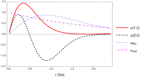
Figure 2: The reduced, normalized, wavefunctions $u(r)=rR(r)$, where $R(r)$ is the radial component of the wavefunction, $\Psi(r)=R(r)\,Y_{\ell m}$. For standard $1S$ and $2S$ charmonia, the reduced normalized functions are $u(1S)$ and $u(2S)$, and for the $c\bar{c}$ component in the universal molecular wavefunction discussed in Section 4, we plot the normalized $u_{\rm mol.}$ in place of $\Psi_{\rm mol.}$. As for the compact tetraquark computed in the Born-Oppenheimer potential in Eq. (9), the reduced wavefunction is $u_{\rm BO}$.

3 Compact Tetraquark radiative decay

The diquark wavefunction $\chi_{{}_{{}_{\text{C}}}}$ is evaluated using the variational principle. The two body hamiltonian $H=K+V$ is assumed to have potential

$$V(r)=-\frac{1}{3}\frac{\alpha_{s}}{r}+{\kappa^{\prime}}\,r\,,$$ (6)

The smallest diquarks are obtained with $\kappa^{\prime}=\kappa$, larger sizes can be obtained by decreasing $\kappa^{\prime}$ down to $\kappa^{\prime}=\frac{1}{4}\kappa$ as predicted in the Born-Oppenheimer picture we use.

A trial wavefunction

$$\chi_{{}_{\text{C}}}(r)=\frac{2{\cal C}^{3/2}}{\sqrt{4\pi}}e^{-{\cal C}r}$$ (7)

is used, with the constant ${\cal C}$ determined by minimizing $(\chi,H\,\chi)/(\chi,\chi)$. In the calculation of the amplitude in Eq. (3), the Born-Oppenheimer wavefunction is used

$$\Psi(R)\to\Psi_{\rm BO}(R)$$ (8)

as computed from the potential

$$V_{\rm BO}(R)=\frac{1}{6}\frac{\alpha_{s}}{R}-2\frac{7\alpha_{s}}{6}I_{1}(R)+\frac{\alpha_{s}}{6}I_{4}(R)+k\,\theta(R-R_{0s})\,(R-R_{0s})$$ (9)

The first term in the BO potential corresponds to the octet repulsion between the two heavy quarks. The term containing the function $I_{1}(R)$ corresponds to $c\bar{q}$ and $q\bar{c}$ interactions, with the Fierz coefficient 7/6 calculated as detailed in[13]. The term containing the $I_{4}(R)$ function describes $q\bar{q}$ interactions, and the same octet coefficient of $1/6$ appearing in the first term is included here. The functions $I_{1}$ and $I_{4}$ are given by

$$I_{1}(R)=\int_{\bm{\xi}}{\chi_{{}_{\text{C}}}(|\bm{\xi}|)^{2}}\frac{1}{|\bm{\xi}-\bm{R}|}$$

$$I_{4}(R)=\int_{\bm{\xi},\bm{\eta}}{\chi_{{}_{\text{C}}}(|\bm{\xi}|)^{2}}\chi_{{}_{\text{C}}}(|\bm{\eta}|)^{2}\frac{1}{|\bm{\xi}-\bm{R}-\bm{\eta}|}$$ (10)

Notice that the functions $I_{1}(R)$ and $I_{4}(R)$ are computed in the generic case in which the light quarks are not found at a single point, like in the origin of Fig. 1. Finally, we include in $V_{\rm BO}$ a confining, linearly rising, potential of the colored diquarks, starting at $R=R_{0s}$. For orientation, we choose $R_{0s}=3\pm 1$ fm, i.e. greater than $2{\cal C}^{-1}$ which is the size where the two orbitals start to separate.

With the given parameters we find that the smallest possible value for ${\cal R}$ in the compact picture is

$${\cal R}_{\rm min}=\frac{{\cal B}(X\to\psi^{\prime}\gamma)}{{\cal B}(X\to\psi\gamma)}=0.95^{+0.01}_{-0.07}$$ (11)

despite the fact that the ratio of the phase space volumes is $\Phi(\psi^{\prime}\gamma)/\Phi(\psi\gamma)=0.26$. The reason for this can partially be captured by comparing the $\Psi_{\rm BO}(R)$ with the charmonium $\Psi(R)$, as done in Fig. 2. Note, however, that the superposition integral (3) includes as well the oscillating factor which is not displayed in Fig. 2. We will return to this point in the discussion Section 5. For the moment observe that the value ${\cal R}_{\rm min}$ is obtained using $\kappa^{\prime}=\kappa$ in (6) which makes the smaller diquarks size $(r_{\rm rms})_{cu}\simeq 0.83$ fm, see Fig. 3. Allowing smaller string tensions $\kappa^{\prime}$ makes looser diquarks, as large as $(r_{\rm rms})_{cu}=1.3$ fm in size, corresponding to $\kappa^{\prime}=\frac{1}{4}k$, see Fig. 3.

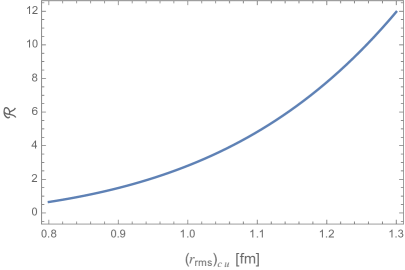
Figure 3: The ratio ${\cal R}$ as a function of the size $(r_{\text{rms}})_{cu}$ of the diquarks in the compact tetraquark picture. For the two values discussed in the text after Eq. (11), ${\cal R}$ varies from ${\cal R}\sim 1$, at $(r_{\text{rms}})_{cu}=0.83$ fm to ${\cal R}\sim 12$, at $(r_{\text{rms}})_{cu}=1.3$ fm.

4 Molecule radiative decay

There is a universal prediction for the $D^{0}\bar{D}^{*0}$ or $\bar{D}^{0}D^{*0}$ wavefunction [19, 20] (see also [21] and especially the discussion in [22])

$$\Psi_{\rm mol.}(R)=\frac{1}{\sqrt{2\pi R_{0}}}\frac{e^{-R/R_{0}}}{R}$$ (12)

where $R_{0}\simeq 1/\sqrt{2mB}$, $B$ being the molecule binding energy. We assume $R_{0}\approx 10$ fm ($B\simeq 200$ KeV) and in the calculation of the amplitude in (3) we substitute

$$\Psi(R)\to\Psi_{\rm mol.}(R)$$ (13)

as given in (12).

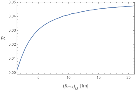
Figure 4: The ratio ${\cal R}$ as a function of the molecular size around the value $(R_{\text{rms}})_{{}_{\text{M}}}=7$ fm ($R_{0}=10$ fm ) discussed in the text.

For the quark orbitals in the $D$ and $D^{*}$ mesons, $\chi_{{}_{\rm{M}}}$, we use Isgur-Scora-Grinstein-Wise (ISGW) functions [23]

$${\chi_{{}_{\rm M}}(r)}=\frac{b^{3/2}}{\pi^{3/4}}e^{-\frac{1}{2}b^{2}r^{2}}$$ (14)

where $b=0.35$ GeV (giving $(r_{\rm rms})_{D,D^{*}}\simeq 0.69\;\text{fm}$) is calculated at the given value of $\alpha_{s}$.

Using $(R_{\rm rms})_{{}_{\text{M}}}=17\;\text{fm}$ and $(r_{\rm rms})_{D,D^{*}}=0.68\;\text{fm}$ we find

$${\cal R}=\frac{{\cal B}(X\to\psi^{\prime}\gamma)}{{\cal B}(X\to\psi\gamma)}=0.036\,.$$ (15)

As can be seen in Fig. 4, this ratio slowly saturates at larger molecular sizes remaining quite smaller than the observed value. The ratio ${\cal R}$ found for the compact tetraquarks, Eq. (11), is therefore at least thirty times larger than that of the molecular picture.

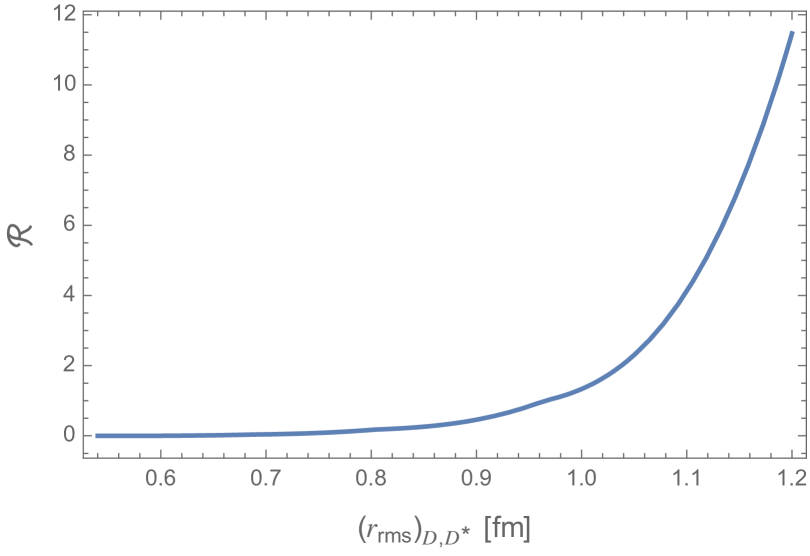
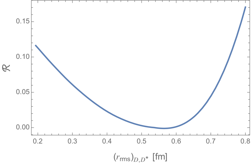
Figure 5: The ratio ${\cal R}$ as a function of the size of the $D$ or $D^{*}$ meson keeping the characteristic size of the molecule $R_{\rm rms}\simeq 7$ fm. The value used in the text is $(r_{\rm rms})_{D,D^{*}}\equiv\sqrt{\langle r^{2}\rangle_{\psi_{{}_{\rm M}}}}\simeq 0.69$ fm. With respect to Fig. 3, the small distance region has a much lower ${\cal R}$ and is flatter.

5 Discussion

The calculation above shows a remarkable disparity in the predictions of the $2S$-to-$1S$ ratio of radiative branching fractions $\mathcal{R}$. Working within the framework explained in Sec. 2, but artificially modifying the wavefunctions, we can investigate the dependence of our results on the specific assumptions of the models used for the compact and molecular pictures of the tetraquark. We will see that the main conclusion, that $\mathcal{R}$ is much bigger for the compact tetraquark than for the molecular picture, is very robust. The detailed shape of the wavefunctions matter little. The determining factor turns out to be the singular nature of the universal wavefunction in the molecular picture, (12), that amplifies the small distance effect and hence the size of the $1S$ amplitude relative to the $2S$ amplitude. As we will see, a factor in reducing $\mathcal{R}$ in the molecular picture relative to the compact tetraquark is the smaller size of the heavy-light systems, that is, that of the $D^{(*)}$ mesons in the molecular case, relative to the size of the diquark in the compact tetraquark picture. Lastly, we will see that in the molecular picture the ratio $\mathcal{R}$ depends quite sensitively on the size of the $1S$ and $2S$ charmonia.

For this exploration we model $\Psi(r)$ in Eq. (3) by the function in Eq. (12) for the molecule, while that of the compact tetraquark by a Single Harmonic Oscillator wave function: $\Psi_{\rm SHO}(r)\sim e^{-\tfrac{1}{2}r^{2}/b^{2}}$. Both of these are functions of a single parameter, the r.m.s. size of the state, $R_{\rm rms}=\sqrt{\langle r^{2}\rangle}$. In addition, $\chi_{{}_{\text{M}}}(r)$ and $\chi_{{}_{\text{C}}}(r)$ are both modeled by $\Psi_{\rm SHO}$ , each characterized by a radius, $r_{\rm rms}=\sqrt{\langle r^{2}\rangle}$ (we denote the size parameters as: $(R_{\text{rms}})_{{}_{\text{M}}}$ and $(r_{\text{rms}})_{D,D^{*}}$ for the molecule, and $(R_{\text{rms}})_{{}_{\text{C}}}$ and $(r_{\text{rms}})_{cu}$ for the compact tetraquark).

For the $\psi(1S)$ and $\psi(2S)$ wavefunctions we use SHO ground and first excited wavefunctions. With $b=0.4\;\text{fm}$ ($r_{\rm rms}=0.49\;\text{fm}$) these are a good approximation to the numerical solutions shown in Fig. 2 that are solutions of the Coulomb plus linear potential.

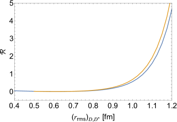
Figure 6: The ratio $\mathcal{R}$ of radiative decay branching fractions as a function of $D^{(*)}$ meson size, computed with the universal wave function $\Psi_{\rm mol.}(r)\sim\exp(-br)/r$ (higher curve) and with a fake molecular function $\Psi(r)\sim\exp(-b^{2}r^{2})/r$ (lower curve). In both cases the hadron size is fixed at $(R_{\rm rms})_{{}_{\text{M}}}=7\;\text{fm}$. The $\psi(1S)$ and $\psi(2S)$ wavefunctions are approximated as ground and first excited state solutions to Schrodinger’s SHO equation, with $r_{\rm rms}=0.5\;\text{fm}$ for the $1S$ state.

To see that the short distance singular structure of the universal wavefunction in the molecular picture is responsible for the small value of the ratio $\mathcal{R}$, we consider a modified $\Psi$ of the form $e^{-\frac{1}{2}b^{2}r^{2}}/r$, that is, an SHO ground state divided by $r$ to amplify the short distance effects. In the absence of the $1/r$ factor this is the wavefunction $\Psi_{\rm SHO}$ of our simplified model for the compact tetraquark.

Fig. 6 shows in blue the resulting ratio $\mathcal{R}$ of this modified wavefunction of the universal wavefunction and in orange the result of the actual universal wavefunction, both as function of the size of the molecule. The curves are remarkably similar, and although quantitatively different, they are both numerically much smaller than the measured value as long as $(r_{\rm rms})_{D,D^{*}}\lesssim 1.1\;\text{fm}$.

Additional evidence that emphasis on the small distance weight of the overlap of wavefunctions produces a very suppressed ratio $\mathcal{R}$ can be seen in Fig. 7, which shows $\mathcal{R}$ in the mock compact tetraquark model as a function of hadron size. As the wavefunction support concentrates around the origin, the contribution to the $1S$ amplitude is accentuated while the one to the $2S$ amplitude is suppressed for small sizes of the $cu$ diquark, like those of $D,D^{*}$ mesons.

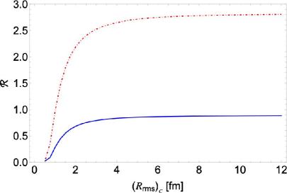
Figure 7: The ratio ${\cal R}$ as a function of the size $(R_{\text{rms}})_{{}_{\text{C}}}$ in the mock model of the compact tetraquark of Sec. 5, assuming $(r_{\text{rms}})_{cu}=(r_{\text{rms}})_{D,D^{*}}=0.69$ fm (continuous curve) or $(r_{\text{{rms}}})_{cu}=0.83$ fm (dot-dashed curve).

Turning to the other parametric dependence, we have already shown that the ratio $\mathcal{R}$ depends quite sensitively on the size $r_{\rm rms}$ of the $\chi_{{}_{\text{M}}}$ and $\chi_{{}_{\text{C}}}$ wavefunctions; see Figs. 3 and 5. We see that for both models the ratio $\mathcal{R}$ increases rapidly with $(r_{\text{rms}})_{cu}$ for $(r_{\text{rms}})_{cu}\gtrsim 0.6\;\text{fm}$, and the molecular model exhibits a minimum in the vicinity of $(r_{\rm rms})_{D,D^{*}}\sim 0.55\;\text{fm}$. This minimum is at $\mathcal{R}=0$: it reflects the vanishing of the $2S$ amplitude at this particular meson size.

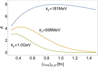
Figure 8: Amplitude for $X$ radiative decay to $\psi(1S)$ (left panel) and $\psi(2S)$ (right panel) as function of $D$-meson or diquark size, for three different values of (artificially modified) photon energy. The curves, in blue, orange and green, have $k=0.181\;\text{GeV}$ (as in the decay to $\psi(2S)$), $0.698\;\text{GeV}$ (as in the decay to $\psi(1S)$), and $1.0\;\text{GeV}$, respectively. This is computed at hadron size $R_{\rm rms}=7\;\text{fm}$ with the approximate charmonium wavefunctions of Sec. 5 at $r_{\rm rms}=0.5\;\text{fm}$.

The rapid growth of these curves can be understood by comparing the $1S$ and $2S$ amplitudes as functions of $r_{\rm rms}$. They both decrease towards zero, but the $1S$ amplitude does faster than the $2S$ amplitude. And the reason for this is that the oscillatory cosine factor in $\eqref{main}$ has shorter wavelength for $1S$ than for $2S$. This can be verified by artificially changing the photon energy $k$ in Eq. (3). Fig. 8 shows the amplitude for $X$ radiative decay to $\psi(1S)$ (left panel) and $\psi(2S)$ (right panel) as function of $D$-meson or diquark size, for three different values of (artificially modified) photon energy: $k=0.181~{}\text{GeV}$ (blue), corresponding to the physical one for the decay into $\psi(2S)$, $0.698\;\text{GeV}$ (orange), corresponding to the physical value for decay to $\psi(1S)$, and $1.0\;\text{GeV}$ (green) corresponding to a lighter than physical final state $\psi(1S)$. In the region $(r_{\rm rms})_{D,D^{*}}\gtrsim 0.5\;\text{fm}$ the physical $1S$ amplitude decreases, becoming negligible for $(r_{\rm rms})_{D,D^{*}}\gtrsim 1.5\;\text{fm}$. At this meson size the physical $2S$ amplitude, while also decreasing, is very sizable, leading to the very enhanced value of $\mathcal{R}$. The advertised zero in the $2S$ amplitude is also made evident by these graphs.

Lastly, we have investigated the dependence of $\mathcal{R}$ in the molecular picture on the size of the final state charmonium states. Fig. 9 shows the ratio $\mathcal{R}$ as a function of molecular size $(R_{\rm rms})_{{}_{\text{M}}}$ (left) and $D^{(*)}$-meson size $(r_{\rm rms})_{D,D^{*}}$, using the approximate wavefunctions described above, for several artificial sizes of the $1S$ and $2S$ states. The left plot, which is computed at meson size $r_{\rm rms}=0.69\;\text{fm}$, shows that $\mathcal{R}$ remains very small and fairly constant as a function of hadron size. The right panel has molecular size $(R_{\rm rms})_{{}_{\text{M}}}=10\;\text{fm}$, although its precise value is irrelevant, as shown by the left panel. One sees that as the size of the charmonium states decreases, the location of the minimum in these curves moves left, towards a smaller value of $(r_{\rm rms})_{D,D^{*}}$. Any attempt to increase $\mathcal{R}$ in the molecular model by decreasing the size of charmonium states by changing the interquark potential would be frustrated by a corresponding decrease in the size of the $D$-meson.

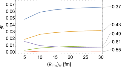
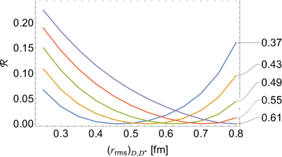
Figure 9: Ratio $\mathcal{R}$ of $2S$ to $1S$ branching fractions in the molecular model as a function of molecular size $(R_{\rm rms})_{{}_{\text{M}}}$ (left) and $D^{(*)}$-meson size $(r_{\rm rms})_{D,D^{*}}$ (right), for several artificially modified sizes of the $1S$ and $2S$ states. The curves are labeled by the rms size (fm) of the $1S$ approximate wavefunction of Sec. 5. The left plot is computed at meson size $(r_{\rm rms})_{D,D^{*}}=0.69\;\text{fm}$ while the right panel has hadron size $(R_{\rm rms})_{{}_{\text{M}}}=7\;\text{fm}$.

6 Conclusions

We have computed the ratio of branching fractions ${\cal R}={\cal B}(X\to\psi^{\prime}\gamma)/{\cal B}(X\to\psi\gamma)$ in the molecular hypothesis following [19, 20], finding ${\cal R}\approx 0.04$, a value much smaller than ${\cal R}_{\rm exp}\simeq 6\pm 4$[12]. While we assume binding energies around $B\sim O(100)$ KeV, leading to molecular sizes of $\sim 10\;\text{fm}$, we show that the result is quite insensitive to the characteristic molecular size. In contrast, $\mathcal{R}$ is a fast increasing functions of the size of the $D^{(*)}$ meson, and our result is obtained for 0.69 fm. The price to pay to get larger ${\cal R}$ values in the molecular hypothesis is that of allowing larger $D$ and $D^{*}$ mesons, well above expectations.

We present a similar calculation for the $X$ described as a compact tetraquark, that is, a diquark-antidiquark color-molecule, treated in the Born-Oppenheimer approximation[13]. We find that the result is also very sensitive to the size of the diquark and not much to the size of the whole tetraquark. This time however, sizes in excess of 0.7 fm are expected, 1 fm not unrealistic. Using the parameters for the compact tetraquark in Ref.[13] we find ${\cal R}\sim 0.95$, about thirty times larger than the predicted value in the molecular model. This value corresponds to the most conservative determination we have (with rms radius $\simeq 0.8$ fm). If we adopt the Casimir scaling of the string tension used to determine the diquark orbitals described in Section 3, and therefore allow slightly larger rms radius, we obtain significantly larger ${\cal R}$ values as in Fig. 3.

The conclusions obtained are rather robust under reasonable parameter variation and even changes in wavefunction shape. Hence, we have found, rather remarkably, that there is a qualitative distinction between what is obtained in the molecular and compact pictures

A better knowledge of the experimental uncertainty in ${\cal R}_{\rm exp}$ would be extremely helpful in clarifying the true nature of the $X(3872)$

References

- [1] A. Esposito, D. Germani, A. Glioti, A. D. Polosa, R. Rattazzi and M. Tarquini, Phys. Lett. B 847 (2023) 138285 [arXiv:2307.11400 [hep-ph]].
- [2] C. Bignamini, B. Grinstein, F. Piccinini, A. D. Polosa and C. Sabelli, Phys. Rev. Lett. 103, 162001 (2009) doi:10.1103/PhysRevLett.103.162001 [arXiv:0906.0882 [hep-ph]].
- [3] P. Artoisenet and E. Braaten, Phys. Rev. D 81, 114018 (2010) doi:10.1103/PhysRevD.81.114018 [arXiv:0911.2016 [hep-ph]].
- [4] A. Esposito, A. L. Guerrieri, L. Maiani, F. Piccinini, A. Pilloni, A. D. Polosa and V. Riquer, Phys. Rev. D 92, no.3, 034028 (2015) doi:10.1103/PhysRevD.92.034028 [arXiv:1508.00295 [hep-ph]].
- [5] A. Esposito, E. G. Ferreiro, A. Pilloni, A. D. Polosa and C. A. Salgado, Eur. Phys. J. C 81, no.7, 669 (2021) doi:10.1140/epjc/s10052-021-09425-w [arXiv:2006.15044 [hep-ph]].
- [6] R. Aaij et al. [LHCb], Phys. Rev. D 102, no.9, 092005 (2020) doi:10.1103/PhysRevD.102.092005 [arXiv:2005.13419 [hep-ex]].
- [7] S. Weinberg, Phys. Rev. 137, B672-B678 (1965) doi:10.1103/PhysRev.137.B672
- [8] A. Esposito, L. Maiani, A. Pilloni, A. D. Polosa and V. Riquer, Phys. Rev. D 105, no.3, L031503 (2022) doi:10.1103/PhysRevD.105.L031503 [arXiv:2108.11413 [hep-ph]].
- [9] M. Ablikim et al. [BESIII], [arXiv:2309.01502 [hep-ex]].
- [10] E. Braaten, L. P. He and J. Jiang, Phys. Rev. D 103, no.3, 036014 (2021) doi:10.1103/PhysRevD.103.036014 [arXiv:2010.05801 [hep-ph]].
- [11] F. K. Guo, C. Hanhart, Y. S. Kalashnikova, U. G. Meißner and A. V. Nefediev, Phys. Lett. B 742, 394-398 (2015) doi:10.1016/j.physletb.2015.02.013 [arXiv:1410.6712 [hep-ph]].
- [12] R. L. Workman et al. [Particle Data Group], PTEP 2022, 083C01 (2022) doi:10.1093/ptep/ptac097
- [13] L. Maiani, A. D. Polosa and V. Riquer, Phys. Rev. D 100, no.1, 014002 (2019) doi:10.1103/PhysRevD.100.014002 [arXiv:1903.10253 [hep-ph]]; See Eq. (5).
- [14] S. Weinberg, Quantum Mechanics, 2nd Ed., Cambridge; page 85.
- [15] H. Xu, N. Yu and Z. Zhang, [arXiv:2401.00411 [hep-ph]].
- [16] see e.g. E. Eichten, K. Gottfried, T. Kinoshita, K. D. Lane and T. M. Yan, Phys. Rev. D 21 (1980), 203 doi:10.1103/PhysRevD.21.203
- [17] N. R. Soni, B. R. Joshi, R. P. Shah, H. R. Chauhan and J. N. Pandya, Eur. Phys. J. C 78 (2018) 592, arXiv:1707.07144 [hep-ph].
- [18] G. S. Bali, Phys. Rept. 343, 1-136 (2001) doi:10.1016/S0370-1573(00)00079-X [arXiv:hep-ph/0001312 [hep-ph]].
- [19] M. B. Voloshin, Phys. Lett. B 579, 316-320 (2004) doi:10.1016/j.physletb.2003.11.014 [arXiv:hep-ph/0309307 [hep-ph]].
- [20] E. Braaten and M. Kusunoki, Phys. Rev. D 69, 074005 (2004) doi:10.1103/PhysRevD.69.074005 [arXiv:hep-ph/0311147 [hep-ph]].
- [21] R. Jackiw, “Delta function potentials in two-dimensional and three-dimensional quantum mechanics,” MIT-CTP-1937, in “Diverse topics in Theoretical and Mathematical Physics”, World Sientific.
- [22] L.D. Landau and E. Lifshitz, Quantum Mechanics, Vol. 3, Pergamon; page 556, Eq. (133.14).
- [23] N. Isgur, D. Scora, B. Grinstein and M. B. Wise, Phys. Rev. D 39, 799-818 (1989) doi:10.1103/PhysRevD.39.799