The Markov-Chain Polytope with Applications

Abstract

This paper addresses the problem of finding a minimum-cost $m$-state Markov chain $(S_{0},\ldots,S_{m-1})$ in a large set of chains. The chains studied have a reward associated with each state. The cost of a chain is its gain, i.e., its average reward under its stationary distribution.

Specifically, for each $k=0,\ldots,m-1$ there is a known set ${\mathbb{S}}_{k}$ of type-$k$ states. A permissible Markov chain contains exactly one state of each type; the problem is to find a minimum-cost permissible chain.

The original motivation was to find a cheapest binary AIFV-$m$ lossless code on a source alphabet of size $n$. Such a code is an $m$-tuple of trees, in which each tree can be viewed as a Markov Chain state. This formulation was then used to address other problems in lossless compression. The known solution techniques for finding minimum-cost Markov chains were iterative and ran in exponential time.

This paper shows how to map every possible type-$k$ state into a type-$k$ hyperplane and then define a Markov Chain Polytope as the lower envelope of all such hyperplanes. Finding a minimum-cost Markov chain can then be shown to be equivalent to finding a “highest” point on this polytope.

The local optimization procedures used in the previous iterative algorithms are shown to be separation oracles for this polytope. Since these were often polynomial time, an application of the Ellipsoid method immediately leads to polynomial time algorithms for these problems.

1 Introduction

Let $\mathbf{S}=(S_{0},S_{1},\ldots,S_{m-1})$ be an $m$-state Markov chain. For convenience $[m]$ will denote the set of indices $\{0,1,\ldots,m-1\}.$ See Figure 1.

For $j,k\in[m],$ let $q_{j}(S_{k})$ be the probability of transitioning from state $S_{k}$ to state $S_{j}$. Assume further that $\forall k\in[m],$ $q_{0}(S_{k})>0.$ Then $\mathbf{S}$ is an ergodic unichain, with one aperiodic recurrent class (containing $S_{0}$) and, possibly, some transient states. $\mathbf{S}$ then has a unique stationary distribution

$$\bm{\pi}(\mathbf{S})=(\pi_{0}(\mathbf{S}),\ldots,\pi_{m-1}(\mathbf{S})).$$

Additionally each state $S_{k}$ has an associated reward or cost $\ell(S_{k});$ the average steady-state cost or gain of $\mathbf{S}$ is defined [8] as

$${\rm cost}(\mathbf{S})=\sum_{k=1}^{m}\ell(S_{k})\pi_{k}(\mathbf{S}).$$

A state $S_{k}$ is fully defined by the $m+1$ values $q_{j}(S_{k}),k\in[m]$ and $\ell(S_{k}).$

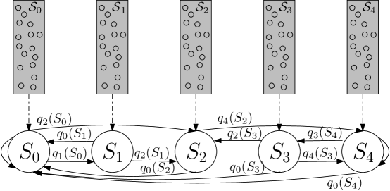
Figure 1: The bottom half of the figure is a five state Markov chain. Arrows represent non-zero transition probabilities. $q_{j}(S_{k})$ is the probability of transitioning from state $S_{k}$ to state $S_{j}.$ Note that $q_{0}(S_{k})>0$ for all $k\in[5].$ The circles in the shaded rectangle ${\mathbb{S}}_{k}$ represent the set of all permissible type-$k$ states with rewards. Each $S_{k}$ in the Markov Chain shown also belongs to the associated set ${\mathbb{S}}_{k}.$

Next suppose that, for each $k\in[m],$ instead of there being only one $S_{k},$ there exists a large set ${\mathbb{S}}_{k}$ containing all permissible “type-$k$’ states”s. Fix

$${\mathbb{S}}=\bigtimes_{k=0}^{m-1}{\mathbb{S}}_{k}=\left\{(S_{0},S_{1},\ldots,S_{m-1})\mid\forall k\in[m],S_{k}\in{\mathbb{S}}_{k}\right\}$$

to be their Cartesian product. ${\mathbb{S}}$ is the set of all permissible Markov chains. The problem is to find the permissible Markov chain with smallest cost.

This problem first arose arose in the context of binary AIFV-$m$ coding [5, 22, 23] (described later in detail in Section 6), in which a code is an $m$-tuple of binary coding trees, $\mathbf{T}=(T_{0},T_{1},\ldots,T_{m-1})$, where there are different rules for each $k$ on how to build the $k$’th coding tree. The cost of the AIFV-$m$ code $\mathbf{T}$ is the cost of a corresponding $m$-state Markov chain, so the problem of finding the minimum-cost binary AIFV-$m$ code reduced to finding a minimum-cost Markov chain [6]. This same minimum-cost Markov chain approach approach was later used to find better parsing trees [17] and lossless codes for finite channel coding [18].

Note that in all of these problems, the input size $n$ was relatively small, e.g., a set of $n$ probabilities, but the associated ${\mathbb{S}}_{k}$ had size exponential in $n.$ The previous algorithms developed for solving the problem were iterative ones that moved from Markov chain to Markov chain in $\cal S$, in some non-increasing cost order. For the specific applications mentioned, they ran in exponential (in $n$) time. They also required solving a local optimzation procedure at each step, which was often polynomial time (in $n$).

[9, 10] developed a different approach for solving the binary AIFV-$2$ coding problem, corresponding to a $2$-state Markov chain, in weakly polynomial time using a simple binary search. In those papers they noted that they could alternatively solve the problem in weakly polynomial time via the Ellipsoid algorithm for linear programming [13] on a two-dimensional polygon. They hypothesized that this latter technique could be extended to $m>2$ but only with a much better understanding of the corresponding multi-dimensional polytopes.

That is the approach followed in this paper, in which we define a mapping of type-$k$ states to type-$k$ hyperplanes in $\mathcal{R}^{m}$. We show that the unique intersection of any $m$ hyperplanes, where each is of a different type, always exists. We call such an intersection point “distinctly-typed” and prove that its “height” is equal to the cost of its associated Markov Chain. The solution to the smallest-cost Markov-Chain problem is thus the lowest height of any “distinctly-typed’ intersection point.

We then define the Markov-Chain polytope $\mathbb{H}$ to be the lower envelope of the hyperplanes associated with all possible permissible states and show that some lowest-height multi-typed intersection point is a highest point on $\mathbb{H}.$ This transforms the problem of finding the cheapest Markov-Chain to the linear programming one of finding a highest point of $\mathbb{H}.$

The construction and observations described above will be valid for ALL Markov chain problems. In the applications mentioned earlier the polytope $\mathbb{H}$ is defined by an exponential number of constraints. But, observed from the proper perspective, the local optimization procedures used at each step of the iterative algorithms in [5, 22, 23, 6, 17] can be repurposed as polynomial time separation oracles for $\mathbb{H}$. This then permits, for example, using the Ellipsoid algorithm approach of [13] to, for any fixed $m,$ solve the AIFV-$m$ problem in weakly polynomial time instead of exponential time.

The remainder of the paper is divided into two distinct parts. Part 1 consists of Sections 2-5. These develop a procedure for solving the generic minimum-cost Markov Chain problem. Section 2 discusses how to map the problem into a linear programming one and how to interpret the old iterative algorithms from this perspective. Section 3 states our new results while Section 4 discusses their algorithmic implications. In particular, Lemma 4.6 states sufficient conditions on ${\mathbb{S}}$ that immediately imply a polynomial time algorithm for finding the minimum cost Markov chain. Section 5 then completes Part 1 by proving the main results stated in Section 3.

Part 2, in Sections 6-8, then discusses how to apply Part 1’s techniques to construct best binary AIFV-$m$ codes in weakly polynomial time

Section 6 provides necessary background, defining binary AIFV-$m$ codes and deriving their important properties. Section 7 describes how to apply the techniques from Section 4 to binary AIFV-$m$ coding. Section 8 proves a very technical lemma specific to binary AIFV-$m$ coding required to show that its associated Markov Chain polytope has a polynomial time separation oracle, which is the last piece needed to apply the Ellipsoid method.

Finally Section 9 concludes with a quick discussion of other applications of the technique and possible directions for going further.

2 Markov Chains

2.1 The Minimum-Cost Markov Chain problem

Definition 2.1.

Fix $m>1.$

• A state $S$ is defined by a set of $m$ transition probabilities $\{q_{j}(S)\}_{j\in[m]}$ along with a cost $\ell(S).$ $\forall{j\in[m]},\,q_{j}(S)\geq 0$ and $\sum_{j\in[m]}q_{j}(S)=1.$

• $\forall k\in[m],\,$ let ${\mathbb{S}}_{k}$ be some finite given set of states satisfying that $\forall S_{k}\in{\mathbb{S}}_{k},\,q_{0}(S_{k})>0.$ The states in ${\mathbb{S}}_{k}$ are known as type-$k$ states.

• Markov Chain $\mathbf{S}=(S_{0},\ldots,S_{m-1})$ is permissible if $\forall k\in[m],\,S_{k}\in{\mathbb{S}}_{k}.$

• ${\mathbb{S}}=\bigtimes_{k=0}^{m-1}{\mathbb{S}}_{k}=\left\{(S_{0},\ldots,S_{m-1})\mid\forall k\in[m],\,S_{k}\in{\mathbb{S}}_{k}\right\}$ is the set of permissible Markov chains

The specific struture of the ${\mathbb{S}}_{k}$ is different from problem to problem. The only universal constraint is that $\forall k\in[m],\,S_{k}\in{\mathbb{S}}_{k},$ $q_{0}(S_{k})>0.$ This condition implies that $\mathbf{S}=(S_{0},\ldots,S_{m-1})$ is an ergodic unichain, with one aperiodic recurrent class (containing $S_{0}$) and, possibly, some transient states. $\mathbf{S}$ therefore has a unique stationary distribution

$$\bm{\pi}(\mathbf{S})=(\pi_{0}(\mathbf{S}),\ldots,\pi_{m-1}(\mathbf{S}))$$

where $\pi_{k}(\mathbf{S})=0$ if and only if $S_{k}$ is a transient state.

Definition 2.2.

Let $\mathbf{S}=(S_{0},S_{1},\ldots,S_{m-1})$ be a permissible $m$-state Markov chain. The average steady-state cost of $\mathbf{S}$ is defined to be

$${\rm cost}(\mathbf{S})=\sum_{k=1}^{m}\ell(S_{k})\pi_{k}(\mathbf{S}).$$

What has been described above is a Markov Chain with rewards, with ${\rm cost}(\mathbf{S})$ being its gain [8].

Definition 2.3.

The minimum-cost Markov chain problem is to find $\mathbf{S}\in{\mathbb{S}}$ satisfying

$${\rm cost}(\mathbf{S})=\min_{\mathbf{S}^{\prime}\in{\mathbb{S}}}{\rm cost}(\mathbf{S}^{\prime}).$$

Note: In the applications motivating this problem, each ${\mathbb{S}}_{k}$ has size exponential in $n,$ so the search space ${\mathbb{S}}$ has size exponential in $mn.$

2.2 Associated Hyperplanes and Polytopes

The next set of definitions map type-$k$ states into type-$k$ hyperplanes in $\mathcal{R}^{m}$ and then defines lower envelopes of those hyperplanes. In what follows, $\mathbf{x}$ denotes a vector $\mathbf{x}=(x_{1},\ldots,x_{m-1})\in\mathcal{R}^{m-1};$ $(\mathbf{x},y)\in\mathcal{R}^{m}$ is a shorthand denoting that $\mathbf{x}\in\mathcal{R}^{m-1}$ and $y\in\mathcal{R}.$ $S_{k}$ denotes a state $S_{k}\in{\mathbb{S}}_{k}.$

The extension to $P$-restricted search spaces is introduced to later (in Lemma 3.5) deal with issues occurring in Markov Chains containing transient states

Definition 2.4 ($P$-restricted search spaces).

$\mathcal{P}$ denotes the set of all subsets of $[m]$ that contain “0”, i.e., $\mathcal{P}=\{P\subseteq[m]\mid 0\in P\}.$

For every state $S,$ define $P(S)=\{j\in[m]\,:\,q_{j}(S)>0\},$ the set of all states to which $S$ can transition. Note that $P(S)\in\mathcal{P}.$

Now fix $k\in[m]$ and $P\in\mathcal{P}.$ Define

$${\mathbb{S}}_{k|P}=\Bigl{\{}S_{k}\in{\mathbb{S}}_{k}\mid P(S_{k})\subseteq P\Bigr{\}}.$$

to be the subset of states in ${\mathbb{S}}_{k}$ that only transition to states in $P.$

Further define

$${\mathbb{S}}_{|P}=\bigtimes_{i=0}^{m-1}{\mathbb{S}}_{k|P}.$$

Note that ${\mathbb{S}}_{k|[m]}={\mathbb{S}}_{k}$ and ${\mathbb{S}}_{|m]}={\mathbb{S}}$. Also note that if $(S_{0},\ldots,S_{m-1})=\mathbf{S}\in{\mathbb{S}}_{|P}$ then, if $k\not\in P,$ $S_{k}$ is a transient state in $\mathbf{S}.$

Definition 2.5.

Let $k\in[m]$ and $P\in\mathcal{P}.$

• Define the type-$k$ hyperplanes $f_{k}:\mathcal{R}^{m-1}\times{\mathbb{S}}_{k}\to\mathcal{R}$ as follows:

  $$f_{0}(\mathbf{x},S_{0}) = \ell(S_{0})+\sum_{j=1}^{m-1}q_{j}(S_{0})\cdot x_{j},$$

  $$\forall k>0,\ f_{k}(\mathbf{x},S_{k}) = \ell(S_{k})+\sum_{j=1}^{m-1}q_{j}(S_{k})\cdot x_{j}-x_{k}.$$

• For all $\mathbf{x}\in\mathcal{R}^{m-1},$ define $g_{k|P}:\mathcal{R}^{m-1}\to\mathcal{R}$ and $S_{k|P}:\mathcal{R}^{m-1}\to{\mathbb{S}}_{k|P}$

  $$g_{k|P}(\mathbf{x}) = \min_{S_{k}\in{\mathbb{S}}_{k|P}}f_{k}(\mathbf{x},S_{k}).$$

  $$\ S_{k|P}(\mathbf{x}) = \arg\min_{S_{k}\in{\mathbb{S}}_{k|P}}f_{k}(\mathbf{x},S_{k}),$$

  and

  $$\mathbf{S}_{|P}(\mathbf{x})=\left(S_{0|P}(\mathbf{x}),S_{1|P}(\mathbf{x})\ldots,S_{m-1|P}(\mathbf{x})\right).$$

  For convenience, $g_{k}(\mathbf{x})$, $S_{k}(\mathbf{x})$ and $\mathbf{S}(\mathbf{x})$ will, respectively, denote $g_{k|[m]}(\mathbf{x})$, $S_{k|[m]}(\mathbf{x})$ and $\mathbf{S}_{|[m]}(\mathbf{x}),$ i.e, all types permitted.

  For later use we note that by definition

  $$\forall\mathbf{x}\in\mathcal{R}^{m-1},\,\forall k\in[m],\ g_{k}(\mathbf{x})=f_{k}\left(\mathbf{x},\,S_{k}(\mathbf{x})\right).$$ (1)

• Finally, for all $\mathbf{x}\in\mathcal{R}^{m-1},$ define.

  $$h(\mathbf{x})=\min_{k\in[m]}g_{k}(\mathbf{x})=\min_{k\in[m]}\min_{S_{k}\in{\mathbb{S}}_{k}}f_{k}(\mathbf{x},S_{k}).$$

$f_{k}$ maps a type-$k$ state $S_{k}$ to a type-$k$ hyperplane $f_{k}(\mathbf{x},S_{k})$ in $\mathcal{R}^{m}.$ For fixed $k,$ $g_{k}(\mathbf{x})$ is the lower envelope of all of the type-$k$ hyperplanes $f_{k}(\mathbf{x},S_{k}).$

Each $S_{k}(\mathbf{x})$ maps point $\mathbf{x}\in\mathcal{R}^{m-1}$ to the lowest a type-$k$ hyperplane evaluated at $\mathbf{x}.$ $\mathbf{S}(\mathbf{x})$ maps point $\mathbf{x}\in\mathcal{R}^{m-1}$ to the Markov chain $\mathbf{S}(\mathbf{x})\in{\mathbb{S}}.$

$h(\mathbf{x})$ will be the lower envelope of the $g_{k}(\mathbf{x})$. Since both $g_{k}(\mathbf{x})$ and $h(\mathbf{x})$ are lower envelopes of hyperplanes they are the upper surface of convex polytopes in $\mathcal{R}^{m}.$ This motivates defining the following polytope:

Definition 2.6.

The Markov Chain Polytope in $\mathcal{R}^{m}$ corresponding to ${\mathbb{S}}$ is

$$\mathbb{H}=\left\{(\mathbf{x},y)\in\mathcal{R}^{m}\mid 0\leq y\leq h(\mathbf{x})\right\}.$$

2.3 The Iterative Algorithm

[5, 6, 22, 23] present an iterative algorithm that was first formulated for finding minimum-cost binary AIFV-$m$ codes and then generalized into a procedure for finding minimum-cost Markov Chains. Although it does not run in polynomial time it is noteworthy because just the fact of its termination (Lemma 2.9) permits later deriving an important property of $\mathbb{H}.$

The complete iterative algorithm is presented as Algorithm 6 and uses the function $F$ defined below:

Definition 2.7.

For $\mathbf{z}\in\mathcal{R}^{m-1}$ define $F(\mathbf{z}):\mathcal{R}^{m-1}\rightarrow\mathcal{R}^{m-1}$ as follows:

1. Find the $m$-tuple of states $\mathbf{S}(\mathbf{z})=\left(S_{0}(\mathbf{z}),S_{1}(\mathbf{z})\ldots,S_{m-1}(\mathbf{z})\right).$

2. Let $\mathbf{z}^{\prime}=(z^{\prime}_{1},z^{\prime}_{2},\ldots,z^{\prime}_{m})$ be the unique intersection point of the $m$ hyperplanes $f_{k}\left(\mathbf{x},S_{k}(\mathbf{z})\right),$ $k\in[m],$ i.e. $\bar{\mathbf{z}}^{\prime}=(z^{\prime}_{1},z^{\prime}_{2},\ldots,z^{\prime}_{m-1})$ where

   $$f_{0}\left(\bar{\mathbf{z}}^{\prime},S_{k}(\mathbf{z})\right)=f_{1}\left(\bar{\mathbf{z}}^{\prime},S_{k}(\mathbf{z})\right)=\cdots=f_{m-1}\left(\bar{\mathbf{z}}^{\prime},S_{m-1}(\mathbf{z})\right)=z^{\prime}_{m}.$$

3. Set $F(\mathbf{z})=\bar{\mathbf{z}}^{\prime}$ to be the projection of $\mathbf{z}^{\prime}$ onto $\mathcal{R}^{m-1}.$

1:$\mathbf{x}^{(1)}:=F\left(\mathbf{x}^{(0)}\right)$; $i:=1$

2:while $\mathbf{x}^{(i)}\not=\mathbf{x}^{(i-1)}$ do

3:      $\mathbf{x}^{(i+1)}:=F\left(\mathbf{x}^{(i}\right)$

4:     $i=i+1$

5:end while

6:Return $\left(\mathbf{S}\left(x^{(i}\right)\right)$ $\triangleright$ Returns Minimun Cost Markov Chain

Algorithm 1 $\mbox{Iterate}\left(\mathbf{x}^{(0)}\right):$ Starts with some arbitrary $\mathbf{x}^{(0)}\in\mathcal{R}^{m-1}$

Notes/Comments

• Algorithm 6 does not at first glance look anything like the algorithm in [5, 6, 22, 23], which was not presented in terms of hyperplanes. We claim though, that Algorithm 1 IS their algorithm after a change of variables. This change of variables makes it easier to define the Markov-chain polytope and its properties.

• Line 1 in Definition 2.7: Calculating $S_{k}(\mathbf{x})$ is very problem specific. In applications, finding $S_{k}(\mathbf{x})$ is a combinatorial optimization problem. For example, the first papers on AIFV-$m$ coding [23] and the most current papers on finite-state channel coding [17] use integer linear programming while the more recent papers on both AIFV-$m$ coding [16, 22, 12] and AIVF coding [18] use dynamic programming.

• In line 2 of Definition 2.7, the existence of the unique intersection point $\mathbf{z}^{\prime}$ is non-obvious and must be proven. It is a consequence of the fact that $\mathbf{S}(\mathbf{z})$ has a unique stationary distribution. This is Lemma 3.1 (a).

• It is not obvious that Algorithm 6 must halt. It could loop forever.

  That it always halts is claimed in [5, 22, 23, 18]. The proofs there are actually missing a case but a complete proof of convergence (using our variable space) is also provided in [2]. The proven result is

  Lemma 2.8.

  [2] For Algorithm 6, no matter what the starting value $\mathbf{x}^{(0)}$ there always exists $i$ such that $\mathbf{x}^{(i)}=\mathbf{x}^{(i-1)}.$

• Correctness of the algorithm will follow from from Lemma 2.8 and Theorem 1(b) in [6] which we state in our notation as

  Lemma 2.9.

  If $F(\mathbf{x})=\mathbf{x},$ then $S(\mathbf{x})$ is a minimum-cost Markov chain.

3 The Main Results

This section states our two main lemmas, Lemma 3.1 and Lemma 3.5, and their consequences. Their proofs are deferred to Section 5.

Lemma 3.1 (Geometric Properties).

Let $\mathbf{S}=(S_{0},\ldots,S_{m-1})\in{\mathbb{S}}$ be a permissible Markov Chain.

• The $m$ $(m-1)$-dimensional hyperplanes $y=f_{k}(\mathbf{x},S_{k}),$ $k\in[m],$ intersect at a unique point $(\mathbf{x}^{int},y^{int})\in\mathcal{R}^{m}$.
  We call such a $(\mathbf{x}^{int},y^{int})$ point a distinctly-typed intersection point.

• $\forall\mathbf{x}\in\mathcal{R}^{m-1},\quad y^{int}={\rm cost}(\mathbf{S})=\sum_{k=0}^{m-1}f_{k}(\mathbf{x},S_{k})\cdot\pi_{k}(\mathbf{S}).$

• The intersection point $(\mathbf{x}^{int},y^{int})$ is on or above the lower envelope of the $m$ hyperplanes $f_{k}(\mathbf{x},S_{k}),$ $k\in[m],$ i.e.,

  $$\forall\ \mathbf{x}\in\mathcal{R}^{m-1},\quad y^{int}\geq\min_{k\in[m]}f_{k}(\mathbf{x},S_{k}).$$

• $$\min_{\mathbf{S}\in{\mathbb{S}}}{\rm cost}(\mathbf{S})\geq\max_{\mathbf{x}\in\mathcal{R}^{m-1}}h(\mathbf{x}).$$

The unique intersection point guaranteed by Lemma 3.1 (a) permits proving the following useful equivalence.

Lemma 3.2.

Let $F(\mathbf{z})$ be as introduced in Definition 2.7. Then

$$F(\mathbf{z})=\mathbf{z}\quad\mbox{ if and only if }\quad g_{0}(\mathbf{z})=g_{1}(\mathbf{z})=\cdots=g_{m-1}(\mathbf{z}).$$ (2)

Proof.

If $F(\mathbf{z})=\mathbf{z}$ then, in the notation of Definition 2.7, the unique intersection point of the $f_{k}(\mathbf{x},S_{k}(\mathbf{z}))$ is $(\mathbf{z},z^{\prime}_{m})$ where

$$f_{0}\left(\mathbf{z},S_{k}(\mathbf{z})\right)=f_{1}\left(\mathbf{z},S_{k}(\mathbf{z})\right)=\cdots=f_{m-1}\left(\mathbf{z},S_{m-1}(\mathbf{z})\right)=z^{\prime}_{m}.$$

Since, $\forall k\in[m]\,$ $g_{k}(\mathbf{z})=f_{k}(\mathbf{z},S_{k}(\mathbf{z}),$ this implies $g_{0}(\mathbf{z})=\cdots=g_{m-1}(\mathbf{z}).$

In the other direction, suppose that $g_{0}(\mathbf{z})=g_{1}(\mathbf{z})=\cdots=g_{m-1}(\mathbf{z})=c$ for some $c.$ Thus $\forall k\in[m],$ $f_{k}(\mathbf{z},S_{k}(\mathbf{z}))=g_{k}(\mathbf{z})$ so

$$f_{0}\left(\mathbf{z},S_{k}(\mathbf{z})\right)=f_{1}\left(\mathbf{z},S_{k}(\mathbf{z})\right)=\cdots=f_{m-1}\left(\mathbf{z},S_{m-1}(\mathbf{z})\right)=c.$$

But this implies that $F(\mathbf{z})=\mathbf{z}.$ ∎

From Lemma 3.1 (a) and (b), finding a minimum-cost Markov Chain is equivalent to finding a minimum “height” ($m$’th-coordinate) distinctly-typed intersection point. Lemma 3.1 (d) states that such a point is always on or above $\mathbb{H}.$ From Lemma 3.2 it then immediately follows (this also reproves Lemma 2.9 independently) that

Corollary 3.3.

If $F(\mathbf{x}^{*})=\mathbf{x}^{*}$ then

$${\rm cost}\left(\mathbf{S}(\mathbf{x}^{*})\right) = f_{0}(\mathbf{x}^{*},S_{0}(\mathbf{x}^{*}))=f_{1}(\mathbf{x},^{*}S_{1}(\mathbf{x}^{*}))=\cdots=f_{m-1}(\mathbf{x}^{*},S_{m-1}(\mathbf{x}^{*}))$$

$$= g_{0}(\mathbf{x}^{*})=g_{1}(\mathbf{x}^{*})=\cdots=g_{m-1}(\mathbf{x}^{*})$$

$$= h(\mathbf{x}^{*}).$$

Thus, from Lemma 3.1 (d),

$$h(\mathbf{x}^{*})={\rm cost}(\mathbf{S}(\mathbf{x}^{*}))\geq\min_{\mathbf{S}\in{\mathbb{S}}}{\rm cost}(\mathbf{S})\geq\max_{\mathbf{x}\in\mathcal{R}^{m-1}}h(\mathbf{x})\geq h(\mathbf{x}^{*})$$

so

$$\min_{\mathbf{S}\in{\mathbb{S}}}{\rm cost}(\mathbf{S})={\rm cost}(\mathbf{S}(\mathbf{x}^{*}))=h(\mathbf{x}^{*})=\max_{\mathbf{x}\in\mathcal{R}^{m-1}}h(\mathbf{x}).$$ (3)

Lemma 3.2 says that $F(\mathbf{x}^{*})=\mathbf{x}^{*}$ means that the $m$ different lower envelopes $g_{k}(\mathbf{x})$, $k\in[m],$ must simultaneously intersect at a point $\mathbf{x}^{*}$. It is not a-priori obvious that such an intersection should always exist but Lemma 2.8 implies that it does, immediately proving

Corollary 3.4.

There exists $\mathbf{x}^{*}\in\mathcal{R}^{m-1}$ satisfying Equation (3).

This has almost transformed the minimum-cost Markov chain problem into the linear programming one of finding a highest point in polytope $\mathbb{H}.$ A complication is that the results above do NOT imply that an arbitrary highest point $\mathbf{x}^{\prime}\in\mathbb{H}$ satisfies $\mathbf{S}(\mathbf{x}^{\prime})$ being a minimum-cost Markov chain. They do not even imply that an arbitrary highest vertex $\mathbf{x}^{\prime}\in\mathbb{H}$ satisfies this, since again we would also need the extra requirement of the vertex being a distinctly-typed intersection point. Luckily, it is possible to start with any highest point on $\mathbb{H}$ and prune it to find a distinctly-typed intersection point at the same height.

Lemma 3.5.

Suppose $(\hat{\mathbf{x}},\hat{y})\in\mathbb{H}$ satisfies $\hat{y}=\max\left\{y\,:\,(\mathbf{x},y)\in{\mathbb{H}}\right\}.$

Let $\mathbf{S}^{*}=(S^{*}_{0},S^{*}_{1},\dots,S^{*}_{m-1})$ denote any minimum-cost Markov chain and $P^{*}=\{k:\pi_{k}(\mathbf{S}^{*})>0\},$ the set of its recurrent indices $k$. Let $P\in\mathcal{P}.$ Then

• If $\forall k\in P,$ $g_{k|P}(\hat{\mathbf{x}})=\hat{y}$, then ${\rm cost}\left(\mathbf{S}_{|P}(\hat{\mathbf{x}})\right)=\hat{y}.$
  Equivalently, this implies $\mathbf{S}_{|P}(\hat{\mathbf{x}})$ is a minimum-cost Markov chain.

• If $P^{*}\subseteq P$, then $\{0\}\subseteq P^{*}\subseteq\{k\in P:g_{k|P}(\hat{\mathbf{x}})=\hat{y}\}$.

Corollary 3.6 (Iterative Pruning Yields Optimal Solution).

Suppose $(\hat{\mathbf{x}},\hat{y})\in{\mathbb{H}}$ satisfies $\hat{y}=\max\left\{y\,:\,(\mathbf{x},y)\in{\mathbb{H}}\right\}.$

Then the procedure $\mbox{\rm Prune}(\mathbf{x})$ in Algorithm 6 terminates in at most $m-1$ steps. At termination, $\mathbf{S}_{|R}(\hat{x})$ is a minimum-cost Markov chain.

1:Set $R=[m]$

2:Set $R^{\prime}=\{k\in[m]\mid g_{k|[m]}(\hat{\mathbf{x}})=\hat{y}\}.$

3:while $R^{\prime}\not=R$ do

4:     Set $R=R^{\prime}$

5:     Set $R^{\prime}=\{k\in R\mid g_{k|R}(\hat{\mathbf{x}})=\hat{y}\}.$

6:end while

Algorithm 2 $\mbox{Prune}(\hat{\mathbf{x}}):$ $(\hat{\mathbf{x}},\hat{y})\in{\mathbb{H}}$ where $\hat{y}=\max\left\{y\,:\,(\mathbf{x},y)\in{\mathbb{H}}\right\}.$

Proof.

At the start of the algorithm, $\{0\}\subseteq P^{*}\subseteq[m]=R.$ As long as $R^{\prime}\not=R$, Lemma 3.5 (b) implies that $\{0\}\subseteq P^{*}\subseteq R^{\prime}\subseteq R.$ If $R\not=R^{\prime}$, the size of $R$ decreases, so the process can not run forever. At termination $R^{\prime}=R$ so, from Lemma 3.5 (a), $\mathbf{S}_{|R}(\hat{\mathbf{x}})$ is a minimum-cost Markov chain. ∎

4 Algorithmic Implications

Stating our running times requires introducing further definitions.

Definition 4.1.

Let ${\bf R}=\bigtimes_{k\in[m]}[\ell_{k},r_{k}]$ be a hyperrectangle in $\mathcal{R}^{m-1}.$ Define

• $t_{{\mathbb{S}}}({\bf R})$ is the maximum time required to calculate $\mathbf{S}(\mathbf{x})$ for any $\mathbf{x}\in{\bf R}.$

• $t^{\prime}_{{\mathbb{S}}}({\bf R})$ is the maximum time required to calculate $\mathbf{S}_{|P}(\mathbf{x})$ for any $\mathbf{x}\in{\bf R}$ and any $P\in\mathcal{P}.$

Note that for any ${\bf R},$ $t_{{\mathbb{S}}}({\bf R})\leq t^{\prime}_{{\mathbb{S}}}({\bf R}).$ Also, $t_{{\mathbb{S}}}$ and $t^{\prime}_{{\mathbb{S}}}$ will denote $t_{{\mathbb{S}}}\left(\mathcal{R}^{m-1}\right)$ and $t^{\prime}_{{\mathbb{S}}}\left(\mathcal{R}^{m-1}\right).$

In addition,

• $I$ denotes the number of iterative steps made by Algorithm 6, the iterative algorithm.

The total amount of time required by the iterative algorithm is then $O(I\cdot t_{{\mathbb{S}}}).$ Improvements to the running time of the iterative algorithm have focused on improving $t_{{\mathbb{S}}}$ in specific applications.

For binary AIFV-$m$ coding, of $n$ source-code words, $\mathbf{S}(\mathbf{x})$ was first solved using integer linear programming [23] so $t_{{\mathbb{S}}}$ was exponential time. For the specific case of ${\bf R}=[0,1]^{m-1}$ this was improved to polynomial time using different dynamic programs. More specifically, for $m=2,$ [16] showed that $t_{{\mathbb{S}}}({\bf R})=O(n^{5})$, improved to $O(n^{3})$ by [11]; for $m>2,$ [22] showed that $t_{{\mathbb{S}}}({\bf R})=O(n^{2m+1})$, improved to $O(n^{m+2})$ by [12]. These sped up the running time of the iterative algorithm under the (unproven) assumption that the iterative algorithm always stayed within $\bf R$.

For AIVF codes, [17] propose using a modification of a Dynamic Programming algorithm due to [4], yielding that for any fixed $m$, $t_{{\mathbb{S}}}$ is polynomial time in $D,$ the number of words permitted in the parse dictionary.

In all of these cases, though, the running time of the algorithm is still exponential because $I,$ the number of Markov-chains that need to be iterated through, might be exponential.

Note: Although $t_{{\mathbb{S}}}({\bf R})$ has been studied, nothing was previously knowm about $t^{\prime}_{{\mathbb{S}}}({\bf R}).$ This is simply because there was no previous need to define and construct $\mathbf{S}_{|P}(\mathbf{x})$. In all the known cases in which algorithms for constructing $\mathbf{S}(\mathbf{x})$ exists it is easy to slightly modify them to construct $\mathbf{S}_{|P}(\mathbf{x})$ in the same running time. So $t^{\prime}_{{\mathbb{S}}}({\bf R})=\Theta(t_{{\mathbb{S}}}({\bf R})).$

We now see how the properties of the Markov chain polytope will, under some fairly loose conditions, permit finding the minimum-cost Markov chain problem in polynomial time. This will be done via the Ellipsoid method of Grötschel, Lovász and Schrijver [13, 14, 20], which, given a polynomial time separation oracle for a polytope will, under some loose conditions, permit solving a linear programming problem on the polytope in polynomial time. The main observation is that $\mathbf{S}(\mathbf{x})$ provides a separation oracle for $\mathbb{H},$ so the previous work on improving $t_{{\mathbb{S}}}$ can be reused to derive polynomial time algorithms.

4.1 Separation oracles and $\mathbb{H}$

Recall the definition of a separation oracle.

Definition 4.2 ([20]).

Let $K\subseteq\mathbb{R}^{m}$ be a closed convex set. A separation oracle for $K$ is a procedure that, for any $\mathbf{x}\in\mathbb{R}^{m},$ either reports that $\mathbf{x}\in K$ or, if $\mathbf{x}\not\in K$, returns a hyperplane that separates $\mathbf{x}$ from $K.$ That is, it returns $\mathbf{a}\in\mathbb{R}^{m}$ such that $\forall\mathbf{z}\in K,$ ${\mathbf{a}}^{T}\mathbf{x}>\mathbf{a}^{T}\mathbf{z}.$

$\mathbf{S}(\mathbf{x})$ provides a separation oracle for $\mathbb{H}.$

Lemma 4.3.

Let $m$ be fixed and $\mathbb{H}$ be the Markov Chain polytope. Let $\mathbf{z}=(\mathbf{x},y)\in\mathcal{R}^{m}$. Then knowing $\mathbf{S}(\mathbf{x})=(S_{0}(\mathbf{x}),\dots,S_{m-1}(\mathbf{x}))$ provides a $O(m^{2})$ time algorithm for either reporting that $\mathbf{z}\in\mathbb{H}$ or returning a hyperplane that separates $\mathbf{z}$ from $\mathbb{H}.$

Proof.

$\mathbf{z}\in\mathbb{H}$ if and only if

$$y\leq h(\mathbf{x})=\min_{k\in[m]}\left(\min_{S_{k}\in{\mathbb{S}}_{k}}f_{k}(\mathbf{x},S_{k})\right)=\min_{k\in[m]}g_{k}(\mathbf{x})=\min_{k\in[m]}f_{k}\left(\mathbf{x},S_{k}(\mathbf{x})\right).$$

Thus knowing $\mathbf{S}(\mathbf{x})$ immediately determines whether $\mathbf{z}\in\mathbb{H}$ or not. Furthermore if $\mathbf{z}\not\in\mathbb{H}$, i.e., $y^{\prime}>h(\mathbf{x}),$ let $k^{\prime}\in[m]$ be an index satisfying $f_{k^{\prime}}\left(\mathbf{x},S_{k^{\prime}}(\mathbf{x})\right)=h(\mathbf{x}).$

The hyperplane $y=f_{k^{\prime}}(\mathbf{x},S_{k^{\prime}}(\mathbf{x}))$ then separates $(\mathbf{x},y^{\prime})$ from $\mathbb{H}$ because $y=f_{k^{\prime}}(\mathbf{x},S_{k^{\prime}}(\mathbf{x}))$ is a supporting hyperplane of $\mathbb{H}$ at point $(\mathbf{x},h(\mathbf{x})).$ ∎

4.2 The Ellipsoid Algorithm with Separation Oracles

The ellipsoid method of Grötschel, Lovász and Schrijver [13, 14] states that, given a polynomial-time separation oracle, (even if $K$ is a polytope defined by an exponential number of hyperplanes) an approximate optimal solution to the “convex optimization problem” can be found in polynomial time. If $K$ is a rational polytope, then an exact optimal solution can be found in polynomial time. We follow the formulation of [20] in stating these results.

Definition 4.4 ([20] Section 14.2).

Optimization Problem Let $K$ be a rational polyhedron in $\mathcal{R}^{m}.$ Given the input $\mathbf{c}\in\mathbb{Q}^{m}$ conclude with one of the following:

• give a vector $\mathbf{x}_{0}\in K$ with $\mathbf{c}^{T}\mathbf{x}_{0}=\max\{\mathbf{c}^{T}\mathbf{x}\,|\,\mathbf{x}\in K\}.$

• give a vector $\mathbf{y}_{0}$ in $\mbox{char.cone}\ K$ with $\mathbf{c}^{T}\mathbf{y}_{0}>0.$

• assert that $K$ is empty.

Note that in this definition, $\mbox{char.cone}\ K$ is the characteristic cone of $K.$ The characteristic cone of a bounded polytope is $\{\bf 0\}$ [20][Section 8.2] so, if $K$ is a bounded nonempty polytope, the optimization problem is to find a vector $\mathbf{x}_{0}\in K$ with $\mathbf{c}^{T}\mathbf{x}_{0}=\max\{\mathbf{c}^{T}\mathbf{x}\,|\,\mathbf{x}\in K\}.$

The important result of [13, 14] is

Theorem 4.5 ([20] Corollary 14.1a).

There exists an algorithm ELL such that if ELL is given the input $(m,\varphi,\mbox{\tt SEP},c)$ where:
          $m$ and $\varphi$ are natural numbers and SEP is a separation oracle for some rational polyhedron $K$ in $\mathcal{R}^{m}$, defined by linear inequalities of size at most $\varphi$ and $c\in\mathbb{Q}^{m},$  
then ELL solves the optimization problem for $K$ for the input $c$ in time polynomially bounded by $m$, $\varphi$, the size of $c$ and the running time of $\mbox{\tt SEP}.$

In this statement the size of a linear inequality is the number of bits needed to write the rational coefficients of the inequality, where the number of bits required to write rational $r=p/q$ where $p,q$ are relatively prime integers, is $\lceil\log_{2}p\rceil+\lceil\log_{2}q\rceil.$

4.3 Solving the Minimum-Cost Markov Chain problem.

Combining all of the pieces we can now prove our main result.

Lemma 4.6.

Given ${\mathbb{S}},$ let $\varphi$ be the maximum number of bits required to write any transition probability $q_{i}(S)$ or cost $\ell(S)$ of a permissible state $S$.

Furthermore, assume some known hyper-rectangle ${\bf R}$ with the property that there exists $(\mathbf{x}^{*},y^{*})\in\mathbb{H}$ satisfying $\mathbf{x}^{*}\in{\bf R}$ and $y^{*}=\max\{y^{\prime}\,:\,(\mathbf{x}^{\prime},y^{\prime})\in\mathbb{H}\}$.

Then the minimum-cost Markov chain problem can be solved in time polynomially bounded by $m$, $\varphi$ and $t^{\prime}_{S}({\bf R}).$

Proof.

The original problem statement permitted the state costs $\ell(S)$ to be negative. Without loss of generality we now assume that $\ell(S)\geq 0$ for all permissible states $S\in\bigcup_{k\in[m]}{\mathbb{S}}_{k}.$ If not, we can just add the same positive value to all state costs, making them all non-negative and keeping the minimum-cost Markov chain minimum under the new costs.

Now set $\mathbb{H}^{\prime}=\mathbb{H}\cap{\bf R}^{\prime}$ where ${\bf R}^{\prime}=\left\{(\mathbf{x},y)\,:\,\mathbf{x}\in{\bf R},\,y\geq 0\right\}.$ Since $y^{*}$ is bounded from above by the cost of any permissible Markov chain, $\mathbb{H}^{\prime}$ is a bounded non-empty polytope.

Since $(\mathbf{x}^{*},y^{*})\in\mathbb{H}^{\prime},$ $\max\{y^{\prime}\,:\,(\mathbf{x}^{\prime},y^{\prime})\in\mathbb{H}\}=\max\{y^{\prime}\,:\,(\mathbf{x}^{\prime},y^{\prime})\in\mathbb{H}^{\prime}\}.$

Now consider the following separation oracle for $\mathbb{H}^{\prime}.$ Let $(\mathbf{x},y)\in\mathcal{R}^{m}.$

• In $O(1)$ time, first check whether $y\geq 0.$ If no, then $(\mathbf{x},y)\not\in\mathbb{H}^{\prime}$ and $y=0$ is a separating hyperplane.

• Otherwise, in $O(m)$ time check whether $\mathbf{x}\in{\bf R}.$ If no, $(\mathbf{x},y)\not\in\mathbb{H}^{\prime}$ and a separating hyperplane is just the corresponding side of $\bf R$ that $(\mathbf{x},y)$ is outside of.

• Otherwise, calculate $\mathbf{S}(\mathbf{x})$ in $t_{S}({\bf R})$ time. From Lemma 4.3 this provides a separation oracle.

Consider solving the optimization problem on polytope $K=\mathbb{H}^{\prime}$ with $\mathbf{c}=(0,0,\ldots,0,1)$ to find $(\mathbf{x}_{0},y_{0})\in\mathbb{H}^{\prime}$ satisfying

$$\mathbf{c}^{T}(\mathbf{x}_{0},y_{0})=\max\{\mathbf{c}^{T}(\mathbf{x}^{\prime},y^{\prime})\,:\,(\mathbf{x}^{\prime},y^{\prime})\in\mathbb{H}^{\prime}\}=\max\{y^{\prime}\,:\,(\mathbf{x}^{\prime},y^{\prime})\in\mathbb{H}^{\prime}\}=y^{*}.$$

Since $\mathbb{H}^{\prime}$ is a bounded non-empty polytope we can apply Theorem 4.5 to find such an $(\mathbf{x}_{0},y_{0})$ in time polynomially bounded in $m,$ $\varphi$, and $t_{{\mathbb{S}}}({\bf R}).$

Applying Corollary 3.6 and its procedure $\mbox{\rm Prune}(\mathbf{x}_{0})$ then produces a minimum cost Markov-Chain in another $O(mt^{\prime}_{{\mathbb{S}}}({\bf R}))$ time. The final result follows from the fact that $t_{{\mathbb{S}}}({\bf R})\leq t^{\prime}_{{\mathbb{S}}}({\bf R}).$ ∎

Part 2, starting in Section 6, shows how to apply this Lemma to derive a polynomial time algorithm for constructing minimin cost AIFV-$m$ codes.

5 Proofs of Lemmas 3.1 and 3.5

5.1 Proof of Lemma 3.1

Before starting the proof we note that (a) and the first equality of (b) are, after a change of variables, implicit in the analysis provided in [6] of the convergence of their iterative algorithm. The derivation there is different than the one provided below, though, and is missing intermediate steps that we need for proving our later lemmas.

Proof.

In what follows, $\mathbf{Q}$ denotes $\mathbf{Q}(\mathbf{S})$, the transition matrix associated with $\mathbf{S},$ and $\bm{\pi}$ denotes $\bm{\pi}(\mathbf{S})$, its unique stationary distribution.

To prove (a) observe that the intersection condition

$$y^{int}=f_{0}(\mathbf{x}^{int},S_{0})=f_{1}(\mathbf{x}^{int},S_{1})=\dots=f_{m-1}(\mathbf{x}^{int},S_{m-1})$$ (4)

can be equivalently rewritten as

$$\begin{bmatrix}y^{int}\\ y^{int}\\ \vdots\\ y^{int}\\ \end{bmatrix}=\begin{bmatrix}f_{0}(\mathbf{x}^{int},S_{0})\\ f_{1}(\mathbf{x}^{int},S_{1})\\ \vdots\\ f_{m-1}(\mathbf{x}^{int},S_{m-1})\\ \end{bmatrix},$$ (5)

where the right-hand side of (5) can be expanded into

$$\begin{bmatrix}\ell(S_{0})\\ \ell(S_{1})\\ \vdots\\ \ell(S_{m-1})\\ \end{bmatrix}+\begin{bmatrix}q_{0}(S_{0})&q_{1}(S_{0})&\dots&q_{m-1}(S_{0})\\ q_{0}(S_{1})&q_{1}(S_{1})&\dots&q_{m-1}(S_{1})\\ \vdots&\vdots&\ddots&\vdots\\ q_{0}(S_{m-1})&q_{1}(S_{m-1})&\dots&q_{m-1}(S_{m-1})\\ \end{bmatrix}\begin{bmatrix}0\\ x^{int}_{1}\\ \vdots\\ x^{int}_{m-1}\\ \end{bmatrix}-\begin{bmatrix}0\\ x^{int}_{1}\\ \vdots\\ x^{int}_{m-1}\\ \end{bmatrix}.$$

Equation (5) can therefore be rewritten as

$$-\begin{bmatrix}\ell(S_{0})\\ \ell(S_{1})\\ \vdots\\ \ell(S_{m-1})\\ \end{bmatrix}=\begin{bmatrix}1&q_{1}(S_{0})&\dots&q_{m-1}(S_{0})\\ 1&q_{1}(S_{1})-1&\dots&q_{m-1}(S_{1})\\ \vdots&\vdots&\ddots&\vdots\\ 1&q_{1}(S_{m-1})&\dots&q_{m-1}(S_{m-1})-1\\ \end{bmatrix}\begin{bmatrix}-y^{int}\\ x^{int}_{1}\\ \vdots\\ x^{int}_{m-1}\\ \end{bmatrix},$$ (6)

where the matrix in (6), denoted as $\mathbf{M},$ is $\mathbf{Q}$ after subtracting the identity matrix $\mathbf{I}$ and replacing the first column with $1$s. To prove (a) it therefore suffices to prove that $\mathbf{M}$ is invertible.

The uniqueness of $\bm{\pi}$ implies that the kernel of $\mathbf{Q}-\mathbf{I}$ is $1$-dimensional. Applying the rank-nullity theorem, the column span of $\mathbf{Q}-\mathbf{I}$ is $(m-1)$-dimensional. Since $(\mathbf{Q}-\mathbf{I})\bm{1}_{m}=\mathbf{Q}\bm{1}_{m}-\mathbf{I}\bm{1}_{m}=\bm{1}_{m}-\bm{1}_{m}=\bm{0}_{m}$, each column of $\mathbf{Q}-\mathbf{I}$ is redundant, i.e., removing any column of $\mathbf{Q}-\mathbf{I}$ does not change the column span.

Next, observe that $\bm{\pi}\bm{1}_{m}=1\neq 0,$ implying that $\bm{\pi}^{T}$ is not orthogonal to $\bm{1}_{m}$. In contrast, each vector $\mathbf{v}$ in the column span of $\mathbf{Q}-\mathbf{I}$ is of the form $\mathbf{v}=(\mathbf{Q}-\mathbf{I})\mathbf{x}$ for some $\mathbf{x}\in\mathcal{R}^{m}$, satisfying $\bm{\pi}\mathbf{v}=\bm{\pi}(\mathbf{Q}-\mathbf{I})\mathbf{x}=(\bm{\pi}\mathbf{Q}-\bm{\pi}\mathbf{I})\mathbf{x}=(\bm{\pi}-\bm{\pi})\mathbf{x}=\bm{0}_{m}^{T}\mathbf{x}=0$, implying that $\mathbf{v}$ is orthogonal to $\bm{1}_{m}$. Thus, $\bm{1}_{m}$ is not in the column span of $\mathbf{Q}-\mathbf{I}$.

Combining these two observations, replacing the first column of $\mathbf{Q}-\mathbf{I}$ with $\bm{1}_{m}$ increases the rank of $\mathbf{Q}-\mathbf{I}$ by exactly one. Hence, $\mathbf{M}$ has rank $m$. This shows invertibility, and the proof of (a) follows.

To prove (b) and (c) observe that

$$\bm{\pi}\begin{bmatrix}y^{int}\\ y^{int}\\ \vdots\\ y^{int}\\ \end{bmatrix}=\bm{\pi}\bm{1}_{m}y^{int}=(1)y^{int}=y^{int},$$

and that for all $\mathbf{x}\in\mathcal{R}^{m-1}$,

$$\bm{\pi}\begin{bmatrix}f_{0}(\mathbf{x},S_{0})\\ f_{1}(\mathbf{x},S_{1})\\ \vdots\\ f_{m-1}(\mathbf{x},S_{m-1})\\ \end{bmatrix} =\bm{\pi}\begin{bmatrix}\ell(S_{0})\\ \ell(S_{1})\\ \vdots\\ \ell(S_{m-1})\\ \end{bmatrix}+\bm{\pi}(\mathbf{Q}-\mathbf{I})\begin{bmatrix}0\\ x_{1}\\ \vdots\\ x_{m-1}\\ \end{bmatrix},$$

$$=\begin{bmatrix}\pi(S_{0})\\ \pi(S_{1})\\ \vdots\\ \pi(S_{m-1})\\ \end{bmatrix}^{T}\begin{bmatrix}\ell(S_{0})\\ \ell(S_{1})\\ \vdots\\ \ell(S_{m-1})\\ \end{bmatrix}+{\bf 0}^{S}_{m}\begin{bmatrix}0\\ x_{1}\\ \vdots\\ x_{m-1}\\ \end{bmatrix},$$

$$=\sum_{k=0}^{m-1}\ell(S_{k})\cdot\pi_{k}(\mathbf{S}),$$

$$={\rm cost}(\mathbf{S}).$$

Applying these observations by setting $\mathbf{x}=\mathbf{x}^{int}$ and left-multiplying by $\bm{\pi},$

$$y^{int}=\bm{\pi}\begin{bmatrix}y^{int}\\ y^{int}\\ \vdots\\ y^{int}\\ \end{bmatrix}=\bm{\pi}\begin{bmatrix}f_{0}(\mathbf{x}^{int},S_{0})\\ f_{1}(\mathbf{x}^{int},S_{1})\\ \vdots\\ f_{m-1}(\mathbf{x}^{int},S_{m-1})\\ \end{bmatrix}={\rm cost}(\mathbf{S}).$$

Applying these observations again, it follows that

$$\forall\mathbf{x}\in\mathcal{R}^{m-1},\quad y^{int}=cost(\mathbf{S})=\bm{\pi}\begin{bmatrix}f_{0}(\mathbf{x},S_{0})\\ f_{1}(\mathbf{x},S_{1})\\ \vdots\\ f_{m-1}(\mathbf{x},S_{m-1})\\ \end{bmatrix}=\sum_{k=0}^{m-1}f_{k}(\mathbf{x},S_{k})\cdot\pi_{k}(\mathbf{S})$$

proving (b). Since the transition probabilities $\pi(S_{k})\geq 0$ are non-negative,

$$\forall\mathbf{x}\in\mathcal{R}^{m-1},\quad y^{int}\geq\min_{k\in[m]}f_{k}(\mathbf{x},S_{k})\cdot\sum_{k=0}^{m-1}\pi(S_{k})=\min_{k\in[m]}f_{k}(\mathbf{x},S_{k}),$$

proving (c).

To prove (d) let $\mathbf{S}=(S_{0},\ldots,S_{m-1})\in{\mathbb{S}}$ be any AIFV-$m$ code and $\mathbf{x}\in\mathcal{R}^{m-1}.$ Combining (b) and (c) yields

$${\rm cost}(\mathbf{S})\geq\min_{k\in[m]}f_{k}(\mathbf{x},S_{k})\geq\min_{k\in[m]}g_{k}(\mathbf{x})=h(\mathbf{x}).$$

This immediately implies

$$\min_{\mathbf{S}\in\mathcal{T}(m,n)}{\rm cost}(\mathbf{S})\geq\max_{\mathbf{x}\in\mathcal{R}^{m-1}}h(\mathbf{x}).$$ (7)

∎

5.2 Proof of Lemma 3.5

Proof.

To prove (a) set $\mathbf{S}_{|P}(\hat{\mathbf{x}})=\left(S_{0|P}(\hat{\mathbf{x}}),S_{1|P}(\hat{\mathbf{x}}),\dots,S_{m-1|P}(\hat{\mathbf{x}})\right).$ Assume that, $\forall k\in P,$ $g_{k|P}(\hat{\mathbf{x}})=f_{k}(\hat{\mathbf{x}},S_{k|P}(\hat{\mathbf{x}}))=\hat{y}.$

By definition, $S_{k|P}(\hat{\mathbf{x}})\in{\mathbb{S}}_{k|P}$ cannot transition to any $S_{j}\in{\mathbb{S}}_{j}$ where $j\not\in P$. This implies that

$$\forall k\not\in P,\ \quad\pi_{k}(\mathbf{S}_{|P}(\hat{\mathbf{x}}))=0\quad\implies\quad\sum_{k\in P}\pi_{k}(\mathbf{S}_{|P}(\hat{\mathbf{x}}))=1.$$

Lemma 3.1 (b) then implies

$${\rm cost}(\mathbf{S}_{|P}(\hat{\mathbf{x}})) = \sum_{k=0}^{m-1}f_{k}(\hat{\mathbf{x}},S_{k|P}(\hat{\mathbf{x}}))\cdot\pi_{k}(\mathbf{S}_{|P}(\hat{\mathbf{x}}))$$

$$= \sum_{k\in P}f_{k}(\hat{\mathbf{x}},S_{k|P}(\hat{\mathbf{x}}))\cdot\pi_{k}(\mathbf{S}_{|P}(\hat{\mathbf{x}}))$$

$$= \sum_{k\in P}\hat{y}\cdot\pi_{k}(\mathbf{S}_{|P}(\hat{\mathbf{x}}))$$

$$= \hat{y}.$$

Thus, $\mathbf{S}_{|P}(\hat{\mathbf{x}})$ is a minimum-cost Markov chain.

To prove (b) first note that, by the restrictions on AIFV-$m$ codes, every state $S^{*}_{k}$ has $q_{0}(S^{*}_{k})>0.$ Thus, $\pi(S^{*}_{0})>0$ and $\{0\}\subseteq P^{*}$, as required.

The Markov chain starts in state $S^{*}_{0}$ where $0\in P^{*}$. We claim that if $k\in P^{*}$ and $j\not\in P^{*}$ then $q_{j}(S^{*}_{k})=0.$ If not, $\pi_{j}(\mathbf{S}^{*})\geq\pi_{k}(\mathbf{S}^{*})\cdot q_{j}(S^{*}_{k})>0$, contradicting that $\pi_{j}(\mathbf{S}^{*})=0.$ Thus, $S^{*}_{k}\in{\mathbb{S}}_{k|P^{*}}$ for all $k\in P^{*}$.

Now, suppose that $P^{*}\subseteq P.$ Then, for all $k\in P^{*}$,

$$f_{k}(\hat{\mathbf{x}},S^{*}_{k})\geq g_{k|P^{*}}(\hat{\mathbf{x}})\geq g_{k|P}(\hat{\mathbf{x}})\geq g_{k}(\hat{\mathbf{x}})\geq h(\hat{\mathbf{x}})=\hat{y}.$$ (8)

On the other hand, using Lemma 3.1 (b) and the fact that $\mathbf{S}^{*}$ is a minimum-cost Markov chain,

$$\hat{y}={\rm cost}(\mathbf{S}^{*})=\sum_{k\in P^{*}}f_{k}(\hat{\mathbf{x}},S^{*}_{k})\cdot\pi_{k}(\mathbf{S}^{*})\geq\hat{y}\sum_{k\in P^{*}}\pi_{k}(\mathbf{S}^{*})=\hat{y}.$$ (9)

The left and right hand sides of (9) are the same and $\forall k\in P^{*},\,\pi_{k}(\mathbf{S}^{*})>0,$ so $\forall k\in P^{*},\,f_{k}(\hat{\mathbf{x}},S^{*}_{k})=\hat{y}$.

This in turn forces all the inequalities in (8) to be equalities, i.e., for all $k\in P^{*}$, $g_{k|P}(\hat{\mathbf{x}})=\hat{y}.$

Thus, $P^{*}\subseteq\{k\in P:g_{k|P}(\hat{\mathbf{x}})=\hat{y}\}$, proving (b). ∎

6 A Polynomial Time Algorithm for binary AIFV-$m$ Coding.

This second part of the paper introduces binary AIFV-$m$ codes and then shows how to to use Lemma 4.6 to find a minimum-cost code of this type in time polynomial in $n$, the number of source words to be encoded, and $b,$ the number of bits required to state the probability of any source word.

The remainder of this section defines these codes and their relationship to the iminimum-cost Markov chain problem.

Section 7 describes how to use Lemma 4.6 to find a minimum cost code in polynomial time.

This first requires showing that $\varphi$ is polynomial in $n$ and $b$, which will be straightforward. It also requires identifying a hyperrectangle $\bf R$ that contains a highest point $(\mathbf{x}^{*},y^{*})\in\mathbb{H}$ and for which $t^{\prime}_{{\mathbb{S}}}({\bf R})$ is polynomial in $n$. That is, $\forall\mathbf{x}\in{\bf R},\forall P\in\mathcal{P},$ $\mathbf{S}_{|P}(\mathbf{x})$ can be calculated in polynomial time.

As mentioned at the start of Section 4, as part of improving the running time of the iterative algorithm, [16, 11, 22, 12] showed that, for ${\bf R}=[0,1]^{m-1},$ $t_{{\mathbb{S}}}({\bf R})$ is polynomial time. As will be discussed in Section 7.2, the algorithms there can be easily modified to show that $t^{\prime}_{{\mathbb{S}}}({\bf R})=O\left(t^{\prime}_{{\mathbb{S}}}({\bf R})\right)$.

Using Lemma 4.6 also requires showing that ${\bf R}=[0,1]^{m-1}$ contains some highest point $(\mathbf{x}^{*},y^{*})\in\mathbb{H}$. Proving this is the most technical part of the proof. It combines a case-analysis of the tree structures of AIFV-$m$ trees with the Poincare-Miranda theorem to show that the functions $g_{k}(\mathbf{x}),$ $k\in[m]$ must all mutually intersect at some point in $\mathbf{x}^{\prime}\in[0,1]^{m-1}.$ Such a mutual intersection satisfies Lemma 3.2 and is therefore the optimum point needed. Section 8 develops the tools required for this analysis.

6.1 Background

Consider a stationary memoryless source with alphabet $\Sigma=\{\sigma_{1},\sigma_{2},\dots,\sigma_{n}\}$ in which symbol $\sigma_{i}$ is generated with probability $p_{i}$. Let ${\mathcal{M}}=m_{1}\,m_{2}\,m_{3}\,\ldots$ be a message generated by the source.

Binary compression codes will encode each $\sigma_{i}$ in ${\mathcal{M}}$ using a binary codeword. Huffman codes are known to be “optimal” such codes. More specifically, they are Minimum Average-Cost Binary Fixed-to-Variable Instantaneous codes. “Fixed-to-Variable” denotes that the binary codewords corresponding to the different $\sigma_{i}$ can have different lengths. “Instantaneous”, that, in a bit-by-bit decoding process, the end of a codeword is recognized immediately after its last bit is scanned. The redundancy of a code is the difference between its average-cost and the Shannon entropy $-\sum_{i}p_{i}\log_{2}p_{i}$ of the source. Huffman codes can have worst case redundancy of $1.$

Huffman codes are often represented by a coding tree, with the codewords being the leaves of the tree. A series of recent work [5, 6, 7, 15, 16, 22, 23] introduced Binary Almost-Instantaneous Fixed-to-Variable-$m$ (AIFV-$m$) codes. Section 6.2 provides a complete definition as well as examples. These differ from Huffman codes in that they use $m$ different coding trees. Furthermore, they might require reading ahead $m$-bits before knowing that the end of a codeword has already been reached (hence “almost”-instantaneous). Since AIFV-$m$ codes include Huffman coding as a special case, they are never worse than Huffman codes. Their advantage is that, at least for $m\leq 5,$ they have worst-case redundancy $1/m$ [15, 7], beating Huffman coding.

Historically, AIFV-$m$ codes were preceded by $K$-ary Almost-Instantaneous FV ($K$-AIFV) codes, introduced in [21]. $K$-ary AIFV codes used a $K$ character encoding alphabet; for $K>2$, the procedure used $K-1$ coding trees and had a coding delay of $1$ bit. For $K=2$ it used 2 trees and had a coding delay of $2$ bits.

Binary AIFV-$m$ codes were introduced later in [15]. These are binary codes that are comprised of an $m$-tuple of binary coding trees and have decoding delay of at most $m$ bits. The binary AIFV-$2$ codes of [15] are identical to the $2$-ary AIFV codes of [21].

Constructing optimal $k$-AIFV or binary AIFV-$m$ codes is much more difficult than constructing Huffman codes. [23] described an iterative algorithm for constructing optimal binary AIFV-$2$ codes. [22] generalized this and proved that, for $m=2,3,4,5$, under some general assumptions, this algorithm, would terminate and, at termination would produce an optimal binary AIFV-$m$ code. The same was later proven for $m>5$ by [5] and [22]. This algorithm was later generalized to solve the Minimun Cost Markov chain problem in [6] and is Algorithm 6 described in Section 2.3. As noted there, Algorithm 6 might look different than the one in [6] but it is really the same algorithm in a different, simpler, coordinate space.

6.2 Code Definitions, Encoding and Decoding

Note: In what follows we assume that the input probabilities satisfy $\sum_{i}p_{i}=1$ and that each $p_{i}$ can be represented using $b$ bits, i.e., each probability is a integral multiple of $2^{-b}$. The running time of our algorithm will, for fixed $m,$ be polynomial in $b$ and $n$, i.e., weakly polynomial.

A binary AIFV-$m$ code will be a sequence $(T_{0},T_{1},\dots,T_{m-1})$ of $m$ binary code trees satisfying Definitions 6.1 and 6.2 below. Each $T_{i}$ contains $n$ codewords. Unlike in Huffman codes, codewords can be internal nodes.

Definition 6.1 (Node Types in a Binary AIFV-$m$ Code [15]).

Figure 2. Edges in an AIFV-$m$ code tree are labelled as $0$-edges or $1$-edges. If node $v$ is connected to its child node $u$ via a $0$-edge ($1$-edge) then $u$ is $v$’s $0$-child ($1$-child). We will often identify a node interchangeably with its associated (code)word. For example $0^{2}10$ is the node reached by following the edges $0,0,1,0$ down from the root. Following [15], the nodes in AIFV-$m$ code trees can be classified as being exactly one of 3 different types:

• Complete Nodes. A complete node has two children: a $0$-child and a $1$-child. A complete node has no source symbol assigned to it.

• Intermediate Nodes. A intermediate node has no source symbol assigned to it and has exactly one child. A intermediate node with a $0$-child is called a intermediate-$0$ node; with a $1$-child is called a intermediate-$1$ node

• Master Nodes. A master node has an assigned source symbol and at most one child node. Master nodes have associated degrees:

  • a master node of degree $k=0$ is a leaf.

  • a master node $v$ of degree $k\geq 1$ is connected to its unique child by a $0$-edge. Furthermore it has exactly $k$ consecutive intermediate-$0$ nodes as its direct descendants, i.e., $v\,0^{t}$ for $0<t\leq k$ are intermediate-$0$ nodes while $v\,0^{k+1}$ is not a intermediate-$0$ node.

Figure 2: Node types in a binary AIFV-$3$ code tree: complete node ($C$), intermediate-$0$ and intermediate-$1$ nodes ($I_{0}$, $I_{1}$), master nodes of degrees $0,1,2$ ($M_{0}$, $M_{1}$, $M_{2}$), ($M_{0}$ is a leaf)and non-intermediate-$0$ nodes ($\neg{I_{0}}$). The $\neg{I_{0}}$ nodes can be complete, master, or intermediate-$1$ nodes, depending upon their location in the tree.

Binary AIFV-$m$ codes are now defined as follows:

Definition 6.2 (Binary AIFV-$m$ Codes [15]).

See Figure 3. Let $m\geq 2$ be a positive integer. A binary AIFV-$m$ code is an ordered $m$-tuple of $m$ code trees $(T_{0},T_{1},\dots,T_{m-1})$ satisfying the following conditions:

1. Every node in each code tree is either a complete node, a intermediate node, or a master node of degree $k$ where $0\leq k<m$.

2. For $k\geq 1$, the code tree $T_{k}$ has a intermediate-$1$ node connected to the root by exactly $k$ $0$-edges, i.e., the node $0^{k}$ is a intermediate-$1$ node.

Consequences of the Definitions:

1. Every leaf of a code tree must be a master node of degree $0$. In particular, this implies that every code tree contains at least one master node of degree $0.$

2. Definition 6.2, and in particular Condition (2), result in unique decodability (proven in [15]).

3. For $k\not=1,$ the root of a $T_{k}$ tree is permitted to be a master node. If a root is a master node, the associated codeword is the empty string (Figure 3)! The root of a $T_{1}$ tree cannot be a master node.

4. The root of a $T_{k}$ tree may be a intermediate-$0$ node.

5. For $k>0,$ every $T_{k}$ tree must contain at least one intermediate-$1$ node, the node $0^{k}.$ A $T_{0}$ tree might not contain any intermediate-$1$ node.
   For $k>0,$ the root of a $T_{k}$ tree cannot be a intermediate-$1$ node. The root of a $T_{0}$ tree is permitted to be a intermediate-$1$ node (but see Lemma 8.7).

Figure 3: Example binary AIFV-$3$ code for source alphabet $\left\{a,b,c,d\right\}.$ The small nodes are either complete or intermediate nodes, while the large nodes are master nodes with their assigned source symbols. Note that $T_{2}$ encodes $\hat{a}$, which is at its root, with an empty string!

We now describe the encoding and decoding procedures. These are illustrated in Figures 4 and 5 which demonstrate the unique decodability property of binary AIFV-$m$ codes.

Procedure 6.3 (Encoding of a Binary AIFV-$m$ Code).

A source sequence $\alpha_{1}\alpha_{2}\dots$ is encoded as follows: Set $T=T_{0}$ and $i=1.$

1.	Encode $\alpha_{i}$ using $T$
2.	Let $k$ be the index such that $\alpha_{i}$ is encoded using a degree-$k$ master node in $T$
3.	Set $T=T_{k};$ $i=i+1$
4.	Goto line 1

Figure 4: Encoding $cbab$ using the binary AIFV-$3$ code in Figure 3. The first $c$ is encoded using a degree-$0$ master node (leaf) in $T_{0}$ so the first $b$ is encoded using $T_{0}.$ This $b$ is encoded using a degree-$2$ master node, so $a$ is encoded using $T_{2}.$ $a$ is encoded using a degree-$1$ master node, so the second $b$ is encoded using $T_{1}\ldots.$

Procedure 6.4 (Decoding of a Binary AIFV-$m$ Code).

Let $\beta$ be a binary string that is the encoded message. Set $T=T_{0}$ and $i=1.$

1.	Let $\beta_{i}$ be	longest prefix of $\beta$ that corresponds to a path from the root of $T$
		to some master node $M$ in $T$
2.	Let $k$ be the degree of $M$ (as a master node) in $T$
3.	Set $\alpha_{i}$ to be the source symbol assigned to $\beta_{i}$ in $T$
4.	Remove $\beta_{i}$ from the start of $\beta.$
5.	Set $T=T_{k};$ $i=i+1$
6.	Goto line 1

Figure 5: Decoding $0001010$ using the binary AIFV-$3$ code in Figure 3.

Theorem 6.5 ([15], Theorem 3).

Binary AIFV-$m$ codes are uniquely decodable with delay at most $m$.

6.3 The cost of AIFV-$m$ codes

$$\begin{array}[]{||cc||ccc|ccc|ccc||}\hline\cr i&\sigma_{i}&\ell(T_{0},\sigma_{i})&d(T_{0},\sigma_{i})&w(T_{0},\sigma_{1})&\ell(T_{1},\sigma_{i})&d(T_{1},\sigma_{i})&w(T_{1},\sigma_{1})&\ell(T_{2},\sigma_{i})&d(T_{2},\sigma\_i)&w(T_{2},\sigma_{1})\\ \hline\cr 1&a&1&1&0&1&2&1&0&1&\epsilon\\ \hline\cr 2&b&1&2&1&3&0&010&4&0&0010\\ \hline\cr 3&c&3&0&000&3&0&011&5&0&00110\\ \hline\cr 4&d&4&0&1000&4&0&1000&5&0&00111\\ \hline\cr\end{array}$$

$$\begin{array}[]{|c|ccc|}\hline\cr{j}&\mathcal{M}_{j}(T_{0})&\mathcal{M}_{j}(T_{1})&\mathcal{M}_{j}(T_{2})\\ \hline\cr 0&\{3,4\}&\{2,3,4\}&\{2,3,4\}\\ 1&\{1\}&\emptyset&\{1\}\\ 2&\{2\}&\{1\}&\emptyset\\ \hline\cr\end{array}\quad\begin{array}[]{|c|ccc|}\hline\cr{j}&q_{j}(T_{0})&q_{j}(T_{1})&q_{j}(T_{2})\\ \hline\cr 0&p_{3}+p_{4}&p_{2}+p_{3}+p_{4}&p_{2}+p_{3}+p_{4}\\ 1&p_{1}&0&p_{1}\\ 2&p_{2}&p_{1}&0\\ \hline\cr\end{array}$$

Figure 6: Example of the values introduced in Definition 6.7 when calculated for the AIFV-$3$ code given in Figure 3. $w(T_{k},\sigma_{i})$ in the first table denotes the codeword for $\sigma_{i}$ in code tree $T_{k}.$ Note that the rightmost table on the second row is the transition matrix $\mathbf{Q}(\mathbf{T})$ for the code.

Definition 6.6.

Let $\mathcal{T}_{k}(m,n)$ denote the set of all possible type-$k$ trees that can appear in a binary AIFV-$m$ code on $n$ source symbols. $T_{k}$ will be used to denote a tree $T_{k}\in\mathcal{T}_{k}(m,n)$. Set $\mathcal{T}(m,n)=\bigtimes_{i=0}^{m-1}\mathcal{T}_{k}(m,n)$.

$\mathbf{T}=(T_{0},\ldots,T_{m-1})\in\mathcal{T}(m,n)$ will be a binary AIFV-$m$ code.

Definition 6.7.

Figure 6. Let $T_{k}\in\mathcal{T}_{k}(m,n)$ and $\sigma_{i}$ be a source symbol.

• $\ell(T_{k},\sigma_{i})$ denotes the length of the codeword in $T_{k}$ for $\sigma_{i}$.

• $d(T_{k},\sigma_{i})$ denotes the degree of the master node in $T_{k}$ assigned to $\sigma_{i}$.

• $\ell(T_{k})$ denotes the average length of a codeword in $T_{k}$, i.e.,

  $$\ell(T_{k})=\sum_{i=1}^{n}\ell(T_{k},\sigma_{i})\cdot p_{i}.$$

• $\mathcal{M}_{j}(T_{k})=\{i\in\{1,2,\ldots,n\}:\,d(T_{k},\sigma_{i})=j\}$ is the set of indices of source nodes that are assigned master nodes of degree $j$ in $T_{k}.$ Set

  $${\bf q}\left(T_{k})=(q_{0}(T_{k}),\ldots,q_{m-1}(T_{k})\right)\quad\mbox{ where }\quad\forall j\in[m],\,\ q_{j}(T_{k})=\sum_{i\in\mathcal{M}_{j}(T_{k})}p_{i}.$$

  $\sum_{j\in m}q_{j}(T_{k})=1,$ so ${\bf q}(T_{k})$ is a probability distribution.

If a source symbol is encoded using a degree-$j$ master node in $T_{k}$, then the next source symbol will be encoded using code tree $T_{j}$. Since the source is memoryless, the transition probability of encoding using code tree $T_{j}$ immediately after encoding using code tree $T_{k}$ is $q_{j}(T_{k})$.

Figure 7: Markov chain corresponding to AIFV-$3$ code in Figure 3. Note that $T_{1}$ contains no degree 1 master node, so there is no edge from $T_{1}$ to $T_{1}.$ Similarly, $T_{2}$ contains no degree 2 master node, so there is no edge from $T_{2}$ to $T_{2}.$

This permits viewing the process as a Markov chain whose states are the code trees. Figure 7 provides an example.

From Consequence (a) following Definition 6.2, $\forall k\in[m],$ every $T_{k}\in\mathcal{T}_{k}(m,n)$ contains at least one leaf, so $q_{0}(T_{k})>0$. Thus, as described in Section 2.1 this implies that the associated Markov chain is a unichain whose unique recurrence class contains $T_{0}$ and whose associated transition matrix $\mathbf{Q}$ has a unique stationary distribution $\bm{\pi}$.

Definition 6.8.

Let $\mathbf{T}=(T_{0},\ldots,T_{m-1})\in\mathcal{T}(m,n)$ be some AIFV-$m$ code, $\mathbf{Q}(\mathbf{T})$ be the transition matrix of the associated Markov chain and

$$\bm{\pi}(\mathbf{T})=(\pi_{0}(\mathbf{T}),\ldots,\pi_{m-1}(\mathbf{T}))$$

be $\mathbf{Q}(\mathbf{T})$’s associated unique stationary distribution. Then the average cost of the code is the average length of an encoded symbol in the limit, i.e.,

$${\rm cost}(\mathbf{T})=\sum_{k=0}^{m-1}\ell(T_{k})\cdot\pi_{k}(\mathbf{T}).$$

Definition 6.9 (The Binary AIFV-$m$ Code problem).

Construct a binary AIFV-$m$ code $\mathbf{T}\in\mathcal{T}(m,n)$ with minimum ${\rm cost}(\mathbf{T}),$ i.e.,

$${\rm cost}(\mathbf{T})=\min_{\mathbf{T}^{\prime}\in\mathcal{T}(m,n)}{\rm cost}(\mathbf{T}^{\prime}).$$

This problem is exactly the minimum-cost Markov Chain problem introduced in section Section 2.1 with ${\mathbb{S}}_{k}=\mathcal{T}_{k}(m,n)$. As discussed in the introduction to Section 4 this was originally solved in exponential time by using the iterative algorithm given in Section 2.3.

7 Using Lemma 4.6 to derive a polynomial time algorithm for binary AIFV-$m$ coding

Because the minimum-cost binary AIFV-$m$ coding problem is a special case of the minimum-cost Markov chain problem, Lemma 4.6 can be applied to derive a polynomial time algorithm. In the discussion below working through this application, $T_{k}$ will denote, interchangeably, both a type-$k$ tree and a type-$k$ state with transition probabilities $q_{j}(T_{k})$ and cost $\ell(T_{k}).$ For example, when writing $f_{k}(\mathbf{x},T_{k})$ (as in Definition 2.5), $T_{k}$ will denote the corresponding Markov chain state and not the tree.

Applying Lemma 4.6 requires showing that, for fixed $m,$ the $\varphi$ and $t^{\prime}_{{\mathbb{S}}}({\bf R})$ parameters in its statement are polynomial in $b$ and $n$.

7.1 Showing that $\varphi$ is polynomial in $b,n$ for AIFV-$m$ coding

Recall that $\varphi$ is the maximum number of bits needed to represent the coefficients of any linear inequality defining a constraint of $\mathbb{H}.$

Showing that $\varphi$ is polynomial in $b$ and $n$ is not difficult but will require the following fact proven later in Corollary 8.9
            For all $T_{k}\in\mathcal{T}_{k}(m,n),$ the height of $T_{k}$ is at most $(n-1)(m+1)+1.$

Lemma 7.1.

${\mathbb{H}}$ is defined by inequalities of size $O(mb+\log n+\log m)$ where $b$ is the maximum number of bits needed to encode any of the $p_{i}.$

Proof.

Note that the definition of ${\mathbb{H}}$ can be equivalently written as

$${\mathbb{H}} = \left\{(\mathbf{x},y)\,|\,(\mathbf{x}\in\mathcal{R}^{m-1},\,y\in\mathcal{R},\,y\leq h(\mathbf{x})\right\}$$

$$= \bigcap_{k\in[m]}\ \bigcap_{T_{k}\in\mathcal{T}_{k}(m,n)}\left\{(\mathbf{x},y)\,|\,\mathbf{x}\in\mathcal{R}^{m-1},\,y\in\mathcal{R},\,y\leq f_{k}(\mathbf{x},T_{k})\right\}$$

$$= \bigcap_{k\in[m]}\ \bigcap_{T_{k}\in\mathcal{T}_{k}(m,n)}\left\{(\mathbf{x},y)\,|\,\mathbf{x}\in\mathcal{R}^{m-1},\,y\in\mathcal{R},\,y+x_{k}-\sum_{j=1}^{m-1}q_{j}(T_{k})\cdot x_{j}\leq\ell(T_{k})\right\}$$

where we set $x_{0}\equiv 0$ to provide notational consistency between $k=0$ and $k>0.$ Thus, the linear inequalities defining ${\mathbb{H}}$ are of the form

$$y+x_{k}-\sum_{j=1}^{m-1}q_{j}(T_{k})\cdot x_{j}\leq\ell(T_{k}).$$ (10)

Since each $p_{i}$ can be represented with $b$ bits, $p_{i}=P_{i}2^{-b}$ for some integral $P\in(0,2^{b}).$ This implies that $q_{j}(T_{k})=Q_{j,k}2^{-b}$ for some integral $Q_{j,k}\in[0,2^{b}].$ So the size of each $q_{j}(T_{k})$ is $\leq 2b.$

Corollary 8.9, to be proven later, states that the height of $T_{k}$ is bounded by $(n-1)(m+1)+1\leq n(m+1).$ Thus each $\ell(T_{k},\sigma_{i})\leq n(m+1)$ for all $k,i$ and $\ell(T_{k})=\sum_{i=1}^{n}\ell(T_{k},\sigma_{i})\cdot p_{i}$ can be written as $L_{k}2^{-b}$ for some integral $L_{k}\in\left[1,n(m+1)2^{b}\right].$ Thus, $\ell(T_{k})$ has size $O(b+\log n+\log m).$ Thus, the size of every inequality (10) is at most $O(mb+\log n+\log m).$ ∎

Recall that $m$ is considered fixed. Thus $\varphi=O(b+\log n).$

7.2 Finding Appropriate $\bf R$ and Showing that $t_{{\mathbb{S}}}({\bf R})$ and $t^{\prime}_{{\mathbb{S}}}({\bf R})$ are Polynomial in $b,n$ for AIFV-$m$ Coding

Recall that ${\mathbb{S}}=\mathcal{T}(m,n).$ Fix $m$ and ${\bf R}=[0,1]^{m-1}.$

As discussed at the starts of Section 4 and 6, there are dynamic programming algorithms that for $m=2$ give $t_{{\mathbb{S}}}({\bf R})=O(n^{3})$ [11] and for $m>2,$  $t_{{\mathbb{S}}}({\bf R})=O(n^{m+2})$ [12]. For $\mathbf{x}\not\in{\bf R}$ the best known algorithms for calculating $\mathbf{S}(\mathbf{x})$ use integer linear programming and run in exponential time.

In deriving the polynomial time binary search algorithm for $m=2$, [10] proved that $\mathbf{x}^{*}\in[0,1]$ and could therefore use the $O(n^{3})$ DP time algorithm for $\mathbf{S}(\mathbf{x})$ as a subroutine. We need to prove something similar for $m>2.$

The main tool used will be the following highly technical lemma whose proof is deferred to the next section.

Lemma 7.2.

Let $m$ be fixed, $n\geq 2^{m}-1,$ $\mathbf{x}\in{\bf R}$ and $k\in\{1\,\ldots,\,m-1\}.$ Then

• If $x_{k}=0,$ $g_{0}(\mathbf{x})-g_{k}(\mathbf{x})\leq 0.$

• If $x_{k}=1,$ $g_{k}(\mathbf{x})-g_{0}(\mathbf{x})\leq 0.$

The proof also needs a generalization of the intermediate-value theorem:

Theorem 7.3 (Poincaré-Miranda Theorem [19]).

Let $f_{1},f_{2},\dots,f_{r}:[0,1]^{r}\to\mathcal{R}$ be $r$ continuous functions of $r$ variables $x_{1},x_{2},\dots,x_{r}\in[0,1]$ such that for all indices $i$, $x_{i}=0$ implies that $f_{i}\leq 0$ and $x_{i}=1$ implies that $f_{i}\geq 0$. It follows that there exists a point $(x_{1},x_{2},\dots,x_{r})\in[0,1]^{r}$ such that $\forall i,\,f_{i}(x_{1},\ldots,x_{r})=0$.

Combining the two yields:

Lemma 7.4.

Let $m$ be fixed and $n\geq 2^{m}-1.$ Then there exists $\mathbf{x}^{*}\in{\bf R}$ satisfying

$$g_{0}(\mathbf{x}^{*})=g_{1}(\mathbf{x}^{*})=\dots=g_{m-1}(\mathbf{x}^{*}).$$ (11)

Proof.

Set $r\leftarrow m-1$ and $f_{k}\leftarrow g_{0}-g_{k}$ for all $k\in\{1,\dots,m-1\}$. From Lemma 7.2, if $x_{k}=0$ then $f_{k}(\mathbf{x})\leq 0$ and if $x_{k}=1$ then $f_{k}(\mathbf{x})\geq 0.$ The Poincaré-Miranda theorem then immediately implies the existence of $\mathbf{x}^{*}\in[0,1]^{m-1}$ such that, $\forall k\in\{1,\dots,m-1\},\,g_{0}(\mathbf{x}^{*})=g_{k}(\mathbf{x}^{*})$, i.e., (11). ∎

Lemma 7.4 combined with Lemma 3.2 and Corollary 3.3 immediately show that if $n\geq 2^{m}-1,$ there exists $\mathbf{x}^{*}\in{\bf R}$ satisfying $h(\mathbf{x}^{*})=\max\{y^{\prime}\,:\,(\mathbf{x}^{\prime},y^{\prime})\in\mathbb{H}\}$.

As noted earlier, for $\mathbf{x}\in{\bf R}$ there are dynamic programming algorithms for calculating $\mathbf{S}(\mathbf{x})$ in $O(n^{3})$ time when $m=2$ [11] and $O(n^{m+2})$ when $m>2$ [12]. Thus $t_{{\mathbb{S}}}({\bf R})=O(n^{3})$ for $m=2$ and $t_{{\mathbb{S}}}({\bf R})=O(n^{m+2})$ for $m>2.$

Those dynamic programming algorithms work by building the $T_{k}$ trees top-down. The status of nodes on the bottom level of the partially built tree, i.e., whether they are complete, intermediate nodes or master nodes of a particular degree, is left undetermined. One step of the dynamic programming algorithm then determines (guesses) the status of those bottom nodes and creates a new bottom level of undetermined nodes. It is easy to modify this procedure so that nodes are only assigned a status within some given $P\in\mathcal{P}.$ The modified algorithms would then calculate $\mathbf{S}_{|P}(\mathbf{x})$ in the same running time as the original algorithms, i.e., $O(n^{3})$ time when $m=2$ and $O(n^{m+2})$ when $m>2$. Thus, for $\mathbf{x}\in{\bf R}$, $t^{\prime}_{{\mathbb{S}}}({\bf R})=O\left(t_{{\mathbb{S}}}({\bf R})\right).$

7.3 The Final Polynomial Time Algorithm

Fix $m$ and set ${\bf R}=[0,1]^{m-1}$. Since $m$ is fixed, we may assume that $n\geq 2^{m}-1.$ For smaller $n,$ the problem can be solved in $O(1)$ time by brute force.

In the notation of Lemma 4.6, Section 7.1 shows that $\varphi=O(b+\log n)$ where $b$ is the maximum number of bits needed to encode any of the $p_{i}.$ Section 7.2 shows that $t^{\prime}_{{\mathbb{S}}}({\bf R})=O(n^{3})$ when $m=2$ and $O(n^{m+2})$ when $m>2$ and there always exists $\mathbf{x}^{*}\in{\bf R}$ satisfying $h(\mathbf{x}^{*})=\max\{y^{\prime}\,:\,(\mathbf{x}^{\prime},y^{\prime})\in\mathbb{H}\}$.

Then, from Lemma 4.6, the binary AIFV-$m$ coding problem can be solved in time polynomially bounded by $\varphi$ and $t^{\prime}_{S}({\bf R}),$ i.e., weakly polynomial in the input.

8 Proof of Lemma 7.2 and Corollary 8.9

The polynomial running time of the algorithm rested upon the correctness of the technical Lemma 7.2 and Corollary 8.9. The proof of Lemma 7.2 requires deriving further technical properties of AIFV-$m$ trees. Corollary 8.9 will be a consequence of some of these derivations.

The main steps of the proof of Lemma 7.2 are:

• generalize binary AIFV-$m$ codes trees to extended binary code trees;

• prove Lemma 7.2 for these extended trees;

• convert this back to a proof of the original lemma.

We start by introducing the concept of extended binary code trees.

Definition 8.1 (Extended Binary AIFV-$m$ Codes).

Fix $k\in[m].$ An extended binary AIFV-$m$ code tree $T^{ex}_{k}$ is defined exactly the same as a $T_{k}$ except that it is permitted to have an arbitrary number of leaves assigned the empty symbol $\epsilon,$ which is viewed as having source probability $0.$

Let $\#_{\epsilon}(T^{ex}_{k})$ denote the number of $\epsilon$-labelled leaves in $T^{ex}_{k}.$ Note that if $\#_{\epsilon}(T^{ex}_{k})=0$, then $T^{ex}_{k}\in\mathcal{T}_{k}(m,n)$.

For notational convenience, let $\mathcal{T}^{ex}_{k}(m,n)$, $f^{ex}_{k}(\mathbf{x},T^{ex}_{k})$, and $g^{ex}_{k}(\mathbf{x})$ respectively denote the extended versions of $\mathcal{T}_{k}(m,n)$, $f_{k}(\mathbf{x},T_{k})$, and $g_{k}(\mathbf{x}).$

Lemma 8.2.

For $k\in\{1,2,\dots,m-1\}$, (a) and (b) below always hold:

• There exists a function $T^{\prime}_{0}\,:\,\mathcal{T}^{ex}_{k}(m,n)\rightarrow\mathcal{T}^{ex}_{0}(m,n)$ satisfying

  $$\ell\left(T^{\prime}_{0}\left[T^{ex}_{k}\right]\right)=\ell\left(T^{ex}_{k}\right)\quad\mbox{and}\quad\forall j\in[m],\,q_{j}\left(T^{\prime}_{0}\left[T^{ex}_{k}\right]\right)=q_{j}\left(T^{ex}_{k}\right)$$

• There exists a function $T^{\prime}_{k}\,:\,\mathcal{T}^{ex}_{0}(m,n)\rightarrow\mathcal{T}^{ex}_{k}(m,n)$ satisfying

  $$\ell\left(T^{\prime}_{k}\left[T^{ex}_{0}\right]\right)=\ell\left(T^{ex}_{0}\right)+1\quad\mbox{and}\quad\forall j\in[m],\,q_{j}\left(T^{\prime}_{k}\left[T^{ex}_{0}\right]\right)=q_{j}\left(T^{ex}_{0}\right)$$

Proof.

(a) follows directly from the fact that, from Definition 6.2, $\mathcal{T}_{k}(m,n)\subseteq\mathcal{T}_{0}(m,n)$ so $\mathcal{T}^{ex}_{k}(m,n)\subseteq\mathcal{T}^{ex}_{0}(m,n)$. Thus, simply setting $T^{\prime}_{0}\left[T^{ex}_{t}\right]=T^{ex}_{k}$ satisfes the required conditions.

Figure 8: Illustration of Lemma 8.2 case (b), describing $T^{\prime}_{k}\left[T^{ex}_{0}\right].$ Note that in $T^{\prime}_{k}\left[T^{ex}_{0}\right],$ leaf $0^{k}1$ is labelled with an $\epsilon$ so the tree is in $\mathcal{T}^{ex}_{k}(m,n)$ but not in $\mathcal{T}_{k}(m,n)$.

To see (b), given $T^{ex}_{0}$ consider the tree $T\in\mathcal{T}^{ex}_{0}(m,n)$ whose root is complete, with the left subtree of the root being a chain of $k-1$ intermediate-$0$ nodes, followed by one intermediate-$1$ node, and a leaf node assigned to $\epsilon$, and whose right subtree is $T^{ex}_{0}$. See Figure 8. Setting $T^{\prime}_{k}\left[T^{ex}_{0}\right]=T$ satisfies the required conditions. ∎

This permits proving:

Lemma 8.3.

Let $\mathbf{x}=(x_{1},\ldots,x_{m-1})\in\mathcal{R}^{m-1}.$ Then $\forall k\in\{1,\dots,m-1\},$

$$\mbox{(i) }g^{ex}_{0}(\mathbf{x})\leq g^{ex}_{k}(\mathbf{x})+x_{k}\quad\mbox{and}\quad\mbox{(ii) }g^{ex}_{k}(\mathbf{x})+x_{k}\leq g^{ex}_{0}(\mathbf{x})+1.$$

Proof.

Lemma 8.2 (a) implies that for all $T^{ex}_{k}\in\mathcal{T}^{ex}_{k}(m,n)$,

$$g^{ex}_{0}(\mathbf{x}) \leq f^{ex}_{0}\left(\mathbf{x},T^{\prime}_{0}\left[T^{ex}_{k}\right]\right)$$

$$= \ell\left(T^{\prime}_{0}\left[T^{ex}_{k}\right]\right)+\textstyle\sum_{j=1}^{m-1}q_{j}\left(T^{\prime}_{0}\left[T^{ex}_{k}\right]\right)\cdot x_{j}$$

$$= \ell\left(T^{ex}_{k}\right)+\textstyle\sum_{j=1}^{m-1}q_{j}\left(T^{ex}_{k}\right)\cdot x_{j}$$

$$= f^{ex}_{k}(\mathbf{x},T^{ex}_{k})+x_{k}.$$

Because this is true for all $T^{ex}_{k}\in\mathcal{T}^{ex}_{k}(m,n)$, it immediately implies (i).

Similarly, Lemma 8.2(b) implies that for all $T^{ex}_{0}\in\mathcal{T}^{ex}_{0}(m,n)$,

$$g^{ex}_{k}(\mathbf{x})+x_{k} \leq f^{ex}_{k}\left(\mathbf{x},T^{\prime}_{k}\left(T^{ex}_{0}\right)\right)+x_{k}$$

$$= \ell\left(T^{\prime}_{t}\left[T^{ex}_{0}\right]\right)+\textstyle\sum_{j=1}^{m-1}q_{j}\left(T^{\prime}_{t}\left[T^{ex}_{0}\right]\right)\cdot x_{j}$$

$$= \ell\left(T^{ex}_{0}\right)+\textstyle\sum_{j=1}^{m-1}q_{j}\left(T^{ex}_{0}\right)\cdot x_{j}+1$$

$$= f^{ex}_{0}(\mathbf{x},T^{ex}_{0})+1.$$

Because this is true for all $T^{ex}_{0}\in\mathcal{T}^{ex}_{0}(m,n)$, it immediately implies (ii). ∎

Plugging $x_{k}=0$ into (i) and $x_{k}=1$ into (ii) proves

Corollary 8.4.

Let $\mathbf{x}\in[0,1]^{m-1}$ and $k\in\{1,\ldots,m-1\}.$Then

• If $x_{k}=0,$ $g^{ex}_{0}(\mathbf{x})-g^{ex}_{k}(\mathbf{x})\leq 0.$

• If $x_{k}=1,$ $g^{ex}_{k}(\mathbf{x})-g^{ex}_{0}(\mathbf{x})\leq 0.$

Note that this is exactly Lemma 7.2 but written for extended binary AIFV-$m$ coding trees rather than normal ones.

While it is not necessarily true that $\forall\mathbf{x}\in\mathcal{R}^{m-1},$ $g^{ex}_{k}(\mathbf{x})=g_{k}(\mathbf{x})$, we can prove that if $n$ is large enough, they coincide in the unit hypercube.

Lemma 8.5.

Let $n\geq 2^{m}-1.$ Then, for all $k\in[m]$ and $\forall\mathbf{x}\in[0,1]^{m-1}$, $g^{ex}_{k}(\mathbf{x})=g_{k}(\mathbf{x}).$

Plugging this Lemma into Corollary 8.4 immediately proves Lemma 7.2. It therefore only remains to prove the correctness of Lemma 8.5 .

8.1 Proving Lemma 8.5

The proof of Lemma 8.5 is split into two parts, The first justifies simplifying the structure of AIFV-$m$ trees. The second uses these properties to actually prove the Lemma.

8.1.1 Further Properties of minimum-cost $T_{k}$ trees

Definitions 6.1 and 6.2 are very loose and technically permit many scenarios, e.g., the existence of more than one intermediate-$1$ node in a $T_{k}$ tree or a chain of intermediate-$0$ nodes descending from the root of a $T_{0}$ tree. These scenarios will not actually occur in trees appearing in minimum-cost codes. The next lemma lists some of these scenarios and justifies ignoring them. This will be needed in the actual proof of Lemma 8.5 in Section 8.1.2

Definition 8.6.

A node $v$ is a left node of $T_{k},$ if $v$ corresponds to codeword $0^{t}$ for some $t\geq 0$.

Note that for $k>0,$ $T_{k}$ contains exactly $k+1$ left nodes. With the exception of $0^{k},$ which must be a intermediate-$1$ node, the other left nodes can technically be any of complete, intermediate-$0$ or master nodes. By definition, they cannot be intermediate-$1$ nodes.

Lemma 8.7.

Let $k\in[m]$ and $T^{\prime}_{k}\in\mathcal{T}^{ex}_{k}(m,n).$ Then there exists $T_{k}\in\mathcal{T}^{ex}_{k}(m,n)$ satisfying both

$$\#_{\epsilon}(T_{k})=\#_{\epsilon}(T^{\prime}_{k}),\quad\ell(T_{k})\leq\ell(T^{\prime}_{k})\quad\mbox{and}\quad\forall j\in[m],\,q_{j}(T_{k})=q_{j}(T^{\prime}_{k})$$ (12)

and the following five conditions:

• The root of $T_{k}$ is not a intermediate-$1$ node;

• The root of $T_{0}$ is not a intermediate-$0$ node;

• If $v$ is a intermediate-$1$ node in $T_{k},$ then the parent of $v$ is not a intermediate-$1$ node;

• If $v$ is a non-root intermediate-$0$ node in $T_{k}$, then the parent of $v$ is either a master node or a intermediate-$0$ node;

• If $v$ is a intermediate-$1$ node in $T_{k}$ then $k\not=0$ and $v=0^{k}.$
  Note that this implies that $v$ is the unique intermediate-$1$ node in $T_{k}.$

Proof.

If a $T^{\prime}_{k}$ tree does not satisfy one of conditions (a)-(d) we first show that it can be replaced by a $T_{k}$ tree with one fewer nodes satisfying (12). Since any tree must contain at least $n$ nodes, this process cannot be repeated forever. Thus a tree satisfying all of the conditions (a)-(d) and satisfying (12) must exist.

Before starting we note that none of the transformations described below adds or removes $\epsilon$-leaves so $\#_{\epsilon}(T_{k})=\#_{\epsilon}(T^{\prime}_{k}).$

If condition (a) is not satisfied in $T^{\prime}_{k},$ then, from Consequence (e) following Definition 6.2, $k=0$. Let $r$ be the intermediate-$1$ root of $T_{0}$ and $v$ its child. Create $T_{0}$ by removing $r$ and making $v$ the root. Then (12) is valid (with $\ell(T_{0})<\ell(T^{\prime}_{0})$).

If condition (b) is not satisfied, let $r$ be the intermediate-$0$ root of $T^{\prime}_{0}$ and $v$ its child. Create $T_{0}$ by removing $r$ and making $v$ the root. Then again (12) is valid (with $\ell(T_{0})<\ell(T^{\prime}_{0})$). Note that this argument fails for $k\not=0$ because removing the edge from $r$ to $v$ would remove the node corresponding to word $0^{k}1$ and $T_{k}$ would then no longer be in $\mathcal{T}_{k}(m,n).$

If condition (c) is not satisfied in $T^{\prime}_{k},$ let $u$ be a intermediate-$1$ node in $T^{\prime}_{k}$ whose child $v$ is also a intermediate-$1$ node. Let $w$ be the unique child of $v.$ Now create $T_{k}$ from $T^{\prime}_{k}$ by pointing the $1$-edge leaving $u$ to $w$ instead of $v,$ i.e., removing $v$ from the tree. Then $\ell(T_{k})\leq\ell(T^{\prime}_{k})$ and (12) is valid.

Figure 9: Illustration of transformations in cases (c) and (d) of Lemma 8.7. Note that the illustration of the second subcase of (d) assumes that $v$ is the $1$-child of $u$. The case in which $v$ is the $0$-child is symmetric.

If condition (d) is not satisfied in $T^{\prime}_{k},$ let $v$ be a intermediate-$0$ node in $T^{\prime}_{k}$ and suppose that its parent $u$ is either a intermediate-$1$ node or a complete node. Let $w$ be the unique child of $v.$ Now create $T_{k}$ from $T^{\prime}_{k}$ by taking the pointer from $u$ that was pointing to $v$ and pointing it to $w$ instead, i.e., again removing $v$ from $T^{\prime}_{k}$. Again, $\ell(T_{k})\leq\ell(T^{\prime}_{k})$ and (12) is valid.

We have shown that for any $T^{\prime}_{k},$ there exists a $T_{k}$ satisfying (a)-(d) and (12).

Now assume that conditions (a)-(d) are satisfied in $T^{\prime}_{k},$ but condition (e) is not. From (a), $v$ is not the root of $T_{k}$ so $u,$ the parent of $v,$ exists. Let $w$ be the unique ($1$-child) of $v.$ From (c) and (d) $w$ can not be a intermediate-$1$ or intermediate-$0$ node so $w$ must be either a master node or a complete node.

Now create $T_{k}$ from $T^{\prime}_{k}$ by taking the pointer from $u$ that was pointing to $v$ and pointing it to $w$ instead, i.e., again removing $v$ from $T^{\prime}_{k}.$

Note that after the transformation, it is easy to see that $\ell(T_{k})\leq\ell(T^{\prime}_{k})$ and (12) is valid. It only remains to show that this is a permissible operation on $T_{k}$ trees, i.e., that $T_{k}$ does not violate Condition 2 from Definition 6.2.

There are two cases:

Case 1: $v=0^{r}$ for some $r>0.$

This is not possible for $k>0$ because, for $r>k,$ $0^{r}\not\in T_{k}$ and for $r<k$, $0^{r}$ has a $0$-child so it can not be a intermediate-$1$ node. So, if $v=0^{r}$, $k=0.$ But Condition 2 from Definition 6.2 cannot be violated when $k=0.$

Case 2: $v\not=0^{r}$ for any $r>0.$

If $k=0$ then, as in case 1, Condition 2 from Definition 6.2 cannot be violated. If $k\not=0,$ then the transformation descrived leaves $o^{k}$ as a intermediate-$1$ node so Condition 2 from Definition 6.2 is still not violated.

Figure 10: Illustration of transformation in case (f) of Lemma 8.7. $v$ is always a intermediate-$1$ node and $w$ can be either a master node or a complete node. $z$ is a master node of degree $t$. In the case in whch $u$ is a complete node, $v$ may be either the left or right child of $u.$ Both cases are illustrated.

This operation of removing a intermediate-$1$ node can be repeated until condition (e) is satisfied. ∎

This lemma has two simple corollaries.

Corollary 8.8.

There exists a minimum-cost AIFV-$m$ code $\mathbf{T}=(T_{0},\ldots,T_{m})$ such that $\forall k\in[m],$ tree $T_{k}$ satisfies conditions (a)-(e) of Lemma 8.7.

Proof.

Let $\mathbf{T}^{\prime}=(T^{\prime}_{0},\ldots,T^{\prime}_{m})$ be a minimum cost AIFV-$m$ code. For each $k\in[m]$ let $T_{k}$ be the tree satisfying conditions (a)-(e) and equation (12) and set $\mathbf{T}=(T_{0},\ldots,T^{\prime}_{m}).$ Since $\mathbf{Q}(\mathbf{T})=\mathbf{Q}(\mathbf{T}^{\prime}),$ $\bm{\pi}(\mathbf{T})=\bm{\pi}(\mathbf{T}^{\prime}).$ Since $\forall k,$ $\ell(T_{k})\leq\ell(T^{\prime}_{k})$,

$${\rm cost}(\mathbf{T})=\sum_{k=0}^{m-1}\ell(T_{k})\cdot\pi_{k}(\mathbf{T})=\sum_{k=0}^{m-1}\ell(T_{k})\cdot\pi_{k}(\mathbf{T}^{\prime})\leq\sum_{k=0}^{m-1}\ell(T^{\prime}_{k})\cdot\pi_{k}(\mathbf{T}^{\prime})={\rm cost}(\mathbf{T}^{\prime}).$$

But $\mathbf{T}^{\prime}$ was a minimum-cost AIFV-$m$ code so $\mathbf{T}$ must be one as well. ∎

The corollary implies that we may assume that in our algorithmic procedures, for all $k\in[m],$ we may assume that all $T_{k}\in\mathcal{T}_{k}(m,n)$ satisfy conditions (a)-(e) of Lemma 8.7.

This assumption permits bounding the height of all $T_{k}$ trees. The following corollary was needed in the proof of Lemma 7.1

Corollary 8.9.

For all $T_{k}\in\mathcal{T}_{k}(m,n),$ the height of $T_{k}$ is at most $(n-1)(m+1)+1.$

Proof.

Let $T_{k}\in\mathcal{T}_{k}(m,n)$ satisfy conditions (a)-(e) of Lemma 8.7.

• Let $\ell\geq 1$ be the number of leaves in $T_{k}.$ Since all leaves are master nodes, $T_{k}$ contains $n-\ell$ non-leaf master nodes.

• Every complete node in $T_{k}$ must contain at least one leaf in each of its left and right subtrees, so the number of complete nodes in $T_{k}$ is at most $\ell-1.$

• $T_{k}$ contains no intermediate-$1$ node if $k=0$ and one intermediate-$1$ node if $k>1.$

• Each intermediate-$0$ node in $T_{k}$ can be written as $v0^{t}$ for some non-leaf master node $v$ and $t\leq m.$ So, the total number of intermediate-$0$ nodes in the tree is at most $(n-\ell)m.$

• The total number of non-leaf nodes in the tree is then at most

  $$(n-\ell)+(\ell-1)+1+(n-\ell)m=n+(n-\ell)m\leq n+(n-1)m.$$

Thus any path from a leaf of $T_{k}$ to its root has length at most $n+(n-1)m=(n-1)(m+1)+1.$ ∎

We note that this bound is almost tight. Consider a $T_{0}$ tree which has only one leaf and with all of the other master nodes (including the root) being master nodes of degree $m.$ This tree is just a chain from the root to the unique leaf, and has of length $(n-1)(m+1).$

8.1.2 The Actual Proof of Lemma 8.5

It now remains to prove Lemma 8.5, i.e., that if $n\geq 2^{m}-1,$ then, for all $k\in[m]$ and $\forall\mathbf{x}\in[0,1]^{m-1}$, $g^{ex}_{k}(\mathbf{x})=g_{k}(\mathbf{x}).$

Proof.

(of Lemma 8.5.)

Recall that $\mathcal{T}_{k}(m,n)\subseteq\mathcal{T}^{ex}_{k}(m,n)$ so, $\forall\mathbf{x}\in\mathcal{R}^{m-1},$ $g^{ex}_{k}(\mathbf{x})\leq g_{k}(\mathbf{x}).$

Fix $\mathbf{x}\in[0,1]^{m-1}$. Now let $T^{ex}_{k}\in\mathcal{T}^{ex}_{k}(m,n)$ be a code tree satisfying

• $f^{ex}_{k}(\mathbf{x},T^{ex}_{k})=\min_{T\in\mathcal{T}^{ex}_{k}(m,n)}f^{ex}_{k}(\mathbf{x},T)=g^{ex}_{k}(\mathbf{x})$ and

• among all trees satisfying (i) be a tree minimizing the number of leaves assigned an $\epsilon$.

Because (12) in Lemma 8.7 keeps $q_{j}(T^{ex}_{k})$ the same and can only reduce $\ell(T^{ex}_{k})$ we may also assume that $T^{ex}_{k}$ satisfies conditions (a)-(e) of Lemma 8.7.

Since $f^{ex}_{k}(\mathbf{x},T^{ex}_{k})=g^{ex}_{k}(\mathbf{x})$, to prove the lemma, it thus suffices to show that $T^{ex}_{k}\in\mathcal{T}_{k}(m,n).$ This implies that $g_{k}(\mathbf{x})\leq g^{ex}_{k}(\mathbf{x})$ so $g_{k}(\mathbf{x})=g^{ex}_{k}(\mathbf{x}).$

Suppose to the contrary that $T^{ex}_{k}\not\in\mathcal{T}_{k}(m,n)$, i.e., $T^{ex}_{k}$ contains a leaf $l_{\epsilon}$ assigned an $\epsilon$. Let $a_{\epsilon}$ denote the closest (lowest) non-intermediate-$0$ ancestor of $l_{\epsilon}$ and $b_{\epsilon}$ be the child of $a_{\epsilon}$ that is the root of the subtree containing $l_{\epsilon}.$

By the definition of $a_{\epsilon},$ either $l_{\epsilon}=b_{\epsilon}$ or $l_{\epsilon}=b_{\epsilon}0^{t}$ where $b_{\epsilon}0^{r},$ $0\leq r<t$ are all intermediate-$0$ nodes for some $t>0.$ From Lemma 8.7 (d), if $b_{\epsilon}$ was a intermediate-$0$ node, $a_{\epsilon}$ must be a master node. Thus, if $a_{\epsilon}$ is a complete node or intermediate-$1$ node $b_{\epsilon}=l_{\epsilon}.$ If $a_{\epsilon}$ is a master node, then $b_{\epsilon}=a_{\epsilon}0$ and $l_{\epsilon}=a_{\epsilon}0^{t+1}$ so $a_{\epsilon}$ is a master node of degree $t.$

Now work through the three cases:

• $a_{\epsilon}$ is a complete node and $b_{\epsilon}=l_{\epsilon}:$ (See Figure 11 (i))
  Let $c_{\epsilon}$ be the other child of $a_{\epsilon}$ (that is not $b_{\epsilon}$). Now remove $b_{\epsilon}$. If $c_{\epsilon}$ was not already the $1$-child of $a_{\epsilon},$ make $c_{\epsilon}$ the $1$-child of $a_{\epsilon}.$

  

  Figure 11: Illustration of the first two cases of the proof of Lemma 8.5. In case (i) $a_{\epsilon}$ is complete and $c_{\epsilon}$ can be its $1$-child or its $0$-child. $T^{\prime}$ is the subtree rooted at $c_{\epsilon}.$ In case (ii) $a_{\epsilon}$ is a master node and $\ell_{\epsilon}$ is connected to it via a chain of intermediate-$0$ nodes.

  The above transformation makes $a_{e}$ a intermediate-$1$ node. The resulting tree remains a valid tree in $\mathcal{T}^{ex}_{k}(m,n)$ preserving the same cost $f^{ex}_{k}(\mathbf{x},T^{ex}_{k})$ but reducing the number of leaves assigned to $\epsilon$ by $1$. This contradicts the minimality of $T^{ex}_{k}$, so this case is not possible.

• $a_{\epsilon}$ is a master node of degree $t>0:$ (See Figure 11 (ii))
  Let $\sigma_{i}$ be the source symbol assigned to $a_{\epsilon}.$ Next remove the path from $a_{\epsilon}$ to $l_{\epsilon},$ converting $a_{\epsilon}$ to a leaf, i.e., a master node of degree $0$. This reduces $f^{ex}_{k}(\mathbf{x},T^{ex}_{k})$ by $p_{i}\cdot x^{*}_{t}\geq 0$ and the number of leaves assigned to $\epsilon$ by $1$. The resulting code tree is still in $\mathcal{T}^{ex}_{k}(m,n)$ and contradicts the minimality of $T^{ex}_{k}$, so this case is also not possible.

  

  Figure 12: Illustration of case (iii) of the proof of Lemma 8.5. $a_{\epsilon}=0^{k}$ is a intermediate-$1$ node and $\beta_{\epsilon}=0^{k}1.$ From definition 6.2 (2), this $b_{\epsilon}$ must exist in every $T_{k}$ so it may not be removed. Furthermore, because $n>2^{m+1},$ $T_{k}$ must contain some node $v_{i}$ at depth $\geq m+2$ corresponding to a source symbol. $\sigma_{i}.$

• $a_{\epsilon}$ is a intermediate-$1$ node and $b_{\epsilon}=l_{\epsilon}:$ (See Figure 12)
  From Lemma 8.7 (a) and (f), $k\not=0$ and $a_{\epsilon}=0^{k}$, $b_{\epsilon}=0^{k}1$.

  Then $b_{\epsilon}$ is at depth $k+1$.

  Note that $T^{ex}_{k}$ can contain at most $2^{k+1}-1$ master nodes at depth $\leq k+1.$ Since $\ell_{\epsilon}=0^{k}1$, $T^{ex}_{k}$ can contain at most $2^{k+1}-2$ master nodes corresponding to source symbols at depth $\leq k+1.$ Thus, if $n\geq 2^{m}-1\geq 2^{k+1}-1,$ there must exist a source symbol at depth greater than $k+1$ in $T^{ex}_{k}.$

  Let $\sigma_{i}$ be the deepest source symbol in the tree. From the argument above, it has depth $\ell(T^{ex}_{k},\sigma_{i})\geq k+2.$

  Let $v_{i}$ be the master node to which $\sigma_{i}$ is assigned and $T_{v_{i}}$ the subtree rooted at $v_{i}.$ Now make $b_{\epsilon}$ the root of $T_{v_{i}}$ instead. Next, change $v_{i}$ so that it is a leaf with $\epsilon$ assigned to it.

  The resulting code tree is still in $\mathcal{T}^{ex}_{k}(m,n)$ while $\ell(T^{ex}_{k})$ is reduced by at least $p_{i}$.

  Furthermore, since the degree of all master nodes associated with source symbols remains unchanged, $\sum_{j=1}^{m-1}q_{j}(T^{ex}_{k})\cdot x^{*}_{j}$ remains unchanged.

  Thus $f^{ex}_{k}(\mathbf{x},T^{ex}_{k})$ is decreased by at least $p_{i}$. This contradicts the minimality of $T^{ex}_{k}$, so this subcase is also not possible.

Since all cases yield a contradiction, it follows that $T^{ex}_{k}\in\mathcal{T}_{k}(m,n)$. ∎

9 Conclusion

The first part of this paper introduced the Minimum-Cost Markov Chain problem and its previously known exponential time iterative solutions. We then showed how how to translate it into the problem of finding the highest point in the Markov Chain Polytope $\mathbb{H}.$ In particular, Lemma 4.6 in Section 4.3 identified the problem specific information that is needed to use the Ellipsoid algorithm to solve the Minimum-Cost Markov Chain problem in polynomial time.

This was written in a a very general form so as to be widely applicable. For example, recent work in progress shows that it can be used to derive polynomial time algorithms for AIVF-coding (parsing) [3] and some problems in finite-state channel coding [1], both of which previously could only be solved in exponential time using the iterative algorithm [17, 18].

The second part of the paper restricts itself to binary Almost Instantaneous Fixed-to-Variable-$m$ (AIFV-$m$) codes, which were the original motivation for the Minimum-Cost Markov Chain problem. These are $m$-tuples of coding trees for lossless-coding that can be modelled as a Markov-chain. We derived properties of AIFV-$m$ coding trees that then permitted applying the technique in the first part to develop the first (weakly) polynomial time algorithm for constructing minimum cost AIFV-$m$ codes.

There are still many related open problems to resolve. The first is to note that our algorithm is only weakly polynomial, since its running time is dependent upon the actual sizes needed to encode of the transition probabilities of the Markov Chain states in binary. For example, in AIFV-$m$ coding, this is polynomial in the number of bits needed to encode the probabilities of the words in the source alphabet. An obvious goal would be, for AIFV-$m$ coding, to find a strongly polynomial time algorithm, one whose running time only depends upon $m$ and $n.$

Another direction would be to return to the iterative algorithm approach of [23, 22, 5, 6]. Our new polynomial time algorithm is primarily of theoretical interest and, like most Ellipsoid based algorithms, would be difficult to implement in practice. Perhaps the new geometric understanding of the problem developed here could improve the performance and analysis of the iterative algorithms.

As an example, the iterative algorithm of [5, 6, 22, 23] presented in Section 2.3 can be interpreted as moving from point to point in the set of distinctly-typed intersection points (of associated hyperplanes), never increasing the cost of the associated Markov chain, finally terminating at the lowest point in this set.

This immediately leads to a better understanding of one of the issues with the iterative algorithms for the AIFV-$m$ problem.

As noted in Section 2.3 the algorithm must solve for $\mathbf{S}(\mathbf{x})$ at every step of the algorithm. As noted in Section 4, this can be done in polynomial time of $\mathbf{x}\in[0,1]^{m-1}$ but requires exponential time integer linear programming if $\mathbf{x}\not\in\in[0,1]^{m-1}.$ A difficulty with the iterative algorithm was that it was not able to guarantee that at every step, or even at the final solution, $\mathbf{x}\in[0,1]^{m-1}.$ With our new better understanding of the geometry of the Markov Chain polytope for the AIFV-$m$ problem, it might now be possible to prove that the condition $\mathbf{x}\in[0,1]^{m-1}$ always holds during the algorithm or develop a modified iterative algorithm in which the condition always holds.

References

- [1] Arshia Dadras and Mordecai Golin. New results on coding for finite-state noiseless channels. In preparation.
- [2] Seyedreza Dolatabadi, Mordecai Golin, and Arian Zamani. Further improvements on the construction of binary aifv- codes. In preparation.
- [3] Seyedreza Dolatabadi, Mordecai Golin, and Arian Zamani. A polynomial time algorithm for aivf coding. In preparation.
- [4] Danny Dube and Fatma Haddad. Individually optimal single-and multiple-tree almost instantaneous variable-to-fixed codes. In 2018 IEEE International Symposium on Information Theory (ISIT), pages 2192–2196. IEEE, 2018.
- [5] Ryusei Fujita, Ken-Ichi Iwata, and Hirosuke Yamamoto. An optimality proof of the iterative algorithm for AIFV- codes. In 2018 IEEE International Symposium on Information Theory (ISIT), pages 2187–2191, 2018.
- [6] Ryusei Fujita, Ken-ichi Iwata, and Hirosuke Yamamoto. An iterative algorithm to optimize the average performance of markov chains with finite states. In 2019 IEEE International Symposium on Information Theory (ISIT), pages 1902–1906, 2019.
- [7] Ryusei Fujita, Ken-ichi Iwata, and Hirosuke Yamamoto. On a redundancy of AIFV- codes for m =3,5. In 2020 IEEE International Symposium on Information Theory (ISIT), pages 2355–2359, 2020.
- [8] Robert G Gallager. Discrete stochastic processes. OpenCourseWare: Massachusetts Institute of Technology, 2011.
- [9] Mordecai Golin and Elfarouk Harb. Polynomial time algorithms for constructing optimal aifv codes. In 2019 Data Compression Conference (DCC), pages 231–240, 2019.
- [10] Mordecai Golin and Elfarouk Harb. A polynomial time algorithm for constructing optimal binary aifv-2 codes. IEEE Transactions on Information Theory, 69(10):6269–6278, 2023.
- [11] Mordecai J. Golin and Elfarouk Harb. Speeding up the AIFV-2 dynamic programs by two orders of magnitude using range minimum queries. Theor. Comput. Science., 865:99–118, 2021.
- [12] Mordecai J Golin and Albert John L Patupat. Speeding up AIFV- dynamic programs by orders of magnitude. In 2022 IEEE International Symposium on Information Theory (ISIT), pages 246–251. IEEE, 2022.
- [13] M. Grötschel, L. Lovász, and A. Schrijver. The ellipsoid method and its consequences in combinatorial optimization. Combinatorica, 1(2):169–197, Jun 1981.
- [14] Martin Grötschel, László Lovász, and Alexander Schrijver. Geometric algorithms and combinatorial optimization, volume 2. Springer Science & Business Media, 2012.
- [15] Weihua Hu, Hirosuke Yamamoto, and Junya Honda. Worst-case redundancy of optimal binary AIFV codes and their extended codes. IEEE Transactions on Information Theory, 63(8):5074–5086, 2017.
- [16] Ken-ichi Iwata and Hirosuke Yamamoto. A dynamic programming algorithm to construct optimal code trees of AIFV codes. In 2016 International Symposium on Information Theory and Its Applications (ISITA), pages 641–645, 2016.
- [17] Ken-ichi Iwata and Hirosuke Yamamoto. Aivf codes based on iterative algorithm and dynamic programming. In 2021 IEEE International Symposium on Information Theory (ISIT), pages 2018–2023. IEEE, 2021.
- [18] Ken-Ichi Iwata and Hirosuke Yamamoto. Joint coding for discrete sources and finite-state noiseless channels. In 2022 IEEE International Symposium on Information Theory (ISIT), pages 3327–3332. IEEE, 2022.
- [19] Wladyslaw Kulpa. The Poincaré-Miranda theorem. The American Mathematical Monthly, 104(6):545–550, 1997.
- [20] Alexander Schrijver. Theory of linear and integer programming. John Wiley & Sons, 1998.
- [21] H. Yamamoto and X. Wei. Almost instantaneous FV codes. In 2013 IEEE International Symposium on Information Theory (ISIT), pages 1759–1763, July 2013.
- [22] Hirosuke Yamamoto and Ken-ichi Iwata. An iterative algorithm to construct optimal binary AIFV- codes. In 2017 IEEE Information Theory Workshop (ITW), pages 519–523, 2017.
- [23] Hirosuke Yamamoto, Masato Tsuchihashi, and Junya Honda. Almost instantaneous fixed-to-variable length codes. IEEE Transactions on Information Theory, 61(12):6432–6443, 2015.