Large $N$ expansion of mass deformed ABJM matrix model:
M2-instanton condensation and beyond




Tomoki Nosaka<sup>1


1</sup>: Kavli Institute for Theoretical Sciences, University of Chinese Academy of Sciences, Beijing, China 100190

We find new bilinear relations for the partition functions of the $\text{U}(N)_{k}\times\text{U}(N+M)_{-k}$ ABJ theory with two parameter mass deformation $(m_{1},m_{2})$, which generalize the $\mathfrak{q}$-Toda-like equation found previously for $m_{1}=m_{2}$. By combining the bilinear relations with the Seiberg-like dualities and the duality cascade relations, we can determine the exact values of the partition functions recursively with respect to $N$. This method is more efficient than the exact calculation by the standard TBA-like approach in the Fermi gas formalism. As an application we study the large $N$ asymptotics of the partition function with the mass parameters in the supercritical regime where the large $N$ expansion obtained for small mass parameters is invalid.

1 Introduction and Summary

Worldvolume theory on multiple M2-branes is an important object in studying M-theory, the AdS/CFT correspondence [1] and various dynamics of three-dimensional supersymmetric field theories. Since the worldvolume theory of arbitrary number $N$ of M2-brane was constructed explicitly as a $\text{U}(N)_{k}\times\text{U}(N+M)_{-k}$ ${\cal N}=6$ superconformal Chern-Simons matter theory [2, 3, 4] (which we shall call ABJ theory in this paper), various features of this model such as the reduction to D2-branes [5, 6, 7], supersymmetry enhancement to ${\cal N}=8$ [8, 9, 10, 11], dualities [12, 13] suggested from the IIB brane setup or M-theory picture and classical solution describing M2-M5 bound states [14, 15, 16, 17, 18, 19, 20] have been investigated. The method of supersymmetry localization [21, 22, 23, 24, 25] is also applicable in this model, which allows us to compute various observable protected by the supersymmetry exactly. In particular, since the free energy proportional to $N^{3/2}$, which is characteristic of M2-branes through the AdS/CFT correspondence [26], was reproduced by the supersymmetry localization of the sphere partition function [27, 28], the large $N$ expansion of the partition function of the ABJ theory was studied extensively [29, 30, 31, 32, 33]. The large $N$ asymptotics of the partition function was also studied in different setups such as the theories with longer circular quivers [34, 35, 36, 37, 38, 39], non-circular quivers [40, 41, 42] or non-unitary gauge groups [43] which correspond to M2-branes probing different orbifold backgrounds, as well as in the theories with continuous deformations [44, 45] or on different manifolds [46, 47, 48, 49]. In some of these setups, the localization formula for the partition function can be reorganized into the partition function of an ideal Fermi gas [50, 51, 52, 53]. This allows us to determine the all order perturbative corrections in $1/N$ as well as some part of the non-perturbative corrections in $1/N$ in the ABJ theory [54, 55, 56, 57, 58] and its generalizations [59, 60, 61, 62, 63, 64, 65, 66, 67, 68, 69, 70]. The results of the exact large $N$ expansion also stimulated various researches on the gravity side in the direction of precision holography such as reproducing the logarithmic correction in $1/N$ [71, 72, 73] and the other $1/N$ perturbative corrections [74] which may correspond to the higher derivative correction in supergravity [75, 76, 77, 78, 79, 80, 81, 82] as well as the non-perturbative effects in $1/N$ [83, 84]. There are some attempts to derive the all order $1/N$ perturbative corrections in the gravity side [85, 86] as well. Furthermore, the exact caulculations also have various applications in the recent development in the bootstrap analysis of three dimensional superconformal field theories [87, 88, 89, 90, 91, 92, 93, 94, 95, 96, 97].

In the exact large $N$ expansion mentioned above, the partition function of the ABJ theory and its generalizations was studied mainly without parameter deformation, or with small deformation to extract refined information of the undeformed theory, where it is assumed that the deformation parameter does not change the large $N$ behavior drastically. However, the model with finite deformation can also enjoy interesting phenomena in the large $N$ limit. In this paper we in particular consider the mass deformation of the ABJ theory which preserves part of the ${\cal N}=6$ supersymmetry [98, 99]. When the theory is considered on the flat space, the mass deformation changes the structure of the vacua drastically. In massless case, the vacua is the $8N$ dimensional continuous moduli space corresponding to the position of M2-branes in eleven dimensional spacetime. When mass parameter is turned on, this is lifted to a discrete set of vacua each of which correspond to part of M2-branes sticking to each other and expanding to fuzzy M5-branes due to the Myers’ effect [100]. When the theory is considered on a compact space, the mass parmeter enters through a dimensionless parameter $mr$ ($r$: length scale of the compact manifold) and the drastic change in the case of flat space may suggest that the theory shows qualitatively different behavior at small $mr$ and at large $mr$. In particular, we expect that the mass deformation gives a non-trivial phase structure to this theory in the large $N$ limit.

In this paper we consider the partition function of the mass deformed ABJ theory compactified on $S^{3}$ with $r_{S^{3}}$ set to $1$. By using the supersymmetry localization method, we can reduce the partition function to a $2N+M$ dimensional ordinary integration. Therefore we can analyze the phase structure of the mass deformed ABJ theory by studying the large $N$ expansion of this integration in various parameter regime. Indeed the large $N$ phase structure was first investigated in the ’t Hooft limit $N,M,k\rightarrow\infty$ with $\frac{N}{k}$ and $\frac{N+M}{k}$ kept finite by applying the large $N$ saddle point approximation to this integration [101, 102]. As a result it was fonud that the partition function exhibits an infinite sequence of phase transitions as the mass parameters and the ’t Hooft couplings are varied.

Besides the ’t Hooft limit we can also consider the M-theory limit $N\rightarrow\infty$ with $k$ and $M$ kept finite. The partition function in this limit was studied in [44] by the large $N$ saddle point approximation [28]. Later it was found for $m_{1}=m_{2}=m$ that the large $N$ saddle configuration in the small mass regime, which is a smooth deformation of the one for $m=0$, becomes inconsistent when $m>\pi$ [103, 104]. This suggests that the model exhibits a large $N$ phase transition at $m_{1}=m_{2}=\pi$. Besides the large $N$ saddle point approximation, the partition function of the mass deformed ABJ theory can also be studied by the Fermi gas formalism. The Fermi gas formalism allows us to determine the all order perturbative expansion in $1/N$ [105], whose leading part precisely reproduces the result of the large $N$ saddle point approximation in the small mass regime. On the other hand, through the small $k$ expansion and the finite $N$ exact values, the Fermi gas formalism also gives some access to the $1/N$ non-perturbative effects. In particular, we find that the exponent of one of these non-perturbative effects has negative real part when $\sqrt{m_{1}m_{2}}>\pi$ [105, 106]. This implies that the $1/N$ expansion obtained in the small mass regime is not valid when $\sqrt{m_{1}m_{2}}>\pi$, which is another evidence for the large $N$ phase transition. In these previous works, however, we were not able to figure out the large $N$ behavior of the partition function in the supercritical regime. The only tool to study this regime was the exact/numerical values of the partition function at finite $N\lesssim 10$, which was not sufficient for making a plausible guess for the large $N$ limit.

In this paper we find a new method to study the large $N$ behavior of the prtition function in the supercritical regime. The idea is based on the connection between the partition function of the ABJ theory and $\mathfrak{q}$-discrete Painlevé $\text{III}_{3}$ system ($\mathfrak{q}\text{PIII}_{3}$) found [107]. This connection can be understood from the following reasons. For the ABJ theory without mass deformation, the large $N$ expansion was completely solved including all order non-perturbative corrections in $1/N$ by using the Fermi gas formalism [108, 109, 110]. As a result, it was found that the coefficients of these non-perturbative effects are precisely given by the Gopakumar-Vafa free energy of the refined topological string on local $\mathbb{P}^{1}\times\mathbb{P}^{1}$. Here the local $\mathbb{P}^{1}\times\mathbb{P}^{1}$ arizes from the density matrix of the Fermi gas formalism ${\hat{\rho}}$ through the prescription to identify the classical limit of ${\hat{\rho}}^{-1}=const.$ as the mirror curve of the target $\text{CY}_{3}$. This correspondence, called topological string/spectral theory (TS/ST) correspondence [111, 112], is believed to hold for more general local Calabi-Yau threefolds and matrix models of Fermi gas form and has been tested through various non-trivial examples [113, 114, 115, 116, 117, 118, 119, 120, 121, 122, 123, 124, 125, 126, 127, 128, 129, 130, 131, 132, 133, 134, 135, 136]. Under the framework of the geometric enginerring [137] the partition function of the topological string is identified with the Nekrasov partition function of the five-dimensional ${\cal N}=1$ Yang-Mills theory realized in the M-theory compactified on the Calabi-Yau threefold [138, 139, 140]. These Nekrasov partition functions are known to satisfy non-linear self-consistency equations called blowup equations [141, 142, 143, 144, 145, 146, 147, 148], which suggests that the partition function of the ABJ theory also satisfy a corresponding relation.

More concretely, the correspondence between the partition function of the ABJ theory and $\mathfrak{q}$-Painlevé systems is that the grand partition function of the ABJ theory with respect to the overall rank $N$ satisfies the $\mathfrak{q}$-Painlevé $\text{III}_{3}$ eqaution in the Hirota bilinear form. Here the rank difference $M$ in the ABJ theory is identified with the discrete time of $\mathfrak{q}\text{PIII}_{3}$. Therefore, given the grand partition function at some two values of $M$, say $M=0,1$, the bilinear relations allow us to determine the grand partition function for all the other values of $M$. On the other hand, the fugacity dual to $N$ corresponds to the initial condition which does not appear explicitly in the bilinear equation. Hence by expanding $\mathfrak{q}\text{PIII}_{3}$ in the fugacity and looking at each order in the fugacity, we obtain an infinite set of bilinear relations among the partition function at different $N$ and $M$.

In [149] it was found that the same bilinear relation also exists for the mass deformed ABJ theory when the two mass parameters $m_{1},m_{2}$ are equal to each other by consulting the five-dimensional theory associated with the curve ${\hat{\rho}}^{-1}=const.$. In this paper we further generalize the relation to the case with non-equal mass parameters. Moreover, by combining these relations with additional constraints on the partition function from the Seiberg-like duality [150, 151] and duality cascade [152, 153, 154], we obtain the recursion relation for the partition function with respect to $N$. The recursion relations are simple and purely algebraic, which enables us to calculate the partition function for finite but very large $N$ more efficiently than the standard method of exact calculation based on the TBA-like structure of the density matrix ${\hat{\rho}}$ [155, 156, 54] employed in [149]. By using the exact (or numerical with high precision) values of the partition function thus obtained, we find the following novel properties of the partition function in the supercritical regime $\sqrt{m_{1}m_{2}}>\pi$.

• First, we find that the partition function for generic values of $N$ oscillates rapidly around zero as a functions of the mass parameters in the supercritical regime. This behavior was already observed in [106], for which it was not even obvious whether there is a well defined large $N$ expansion of the partition function or free energy $-\log Z$ in the supercritical regime. However, in this paper we further find that for each $k$ there is an infinite series of special values of ranks $N^{(k)}_{n}$ ($n=1,2,\cdots$) which grows $N^{(k)}_{n}\sim n^{2}$ at large $n$, for which the partition function is positive definite even in the supercritical regime. This allows us to investigate a smooth large $n$ expansion of the free energy on these sequences.

• By focusing on the special ranks $N^{(k)}_{n}$ we completely identify the large mass asymptotics of the free energy for arbitrary value of $n$ as listed in table 1, up to the corrections of order ${\cal O}(e^{-\frac{m_{1}}{2}},e^{-\frac{m_{2}}{2}})$. Curiously, in the large $n$ limit of the formula we find the same power of $n$ as in the subcritical regime, namely $-\log Z(N_{n}^{(k)})\sim m(N^{(k)}_{n})^{3/2}$. Note that our result is very different from a naive guess for a theory with massive matter fields which is $-\log Z\sim-m(\#(\text{matter fields}))\sim N^{2}$ due to the decoupling. The same discrepancy has been observed also in the three dimensional supersymmetric gauge theories without Chern-Simons terms where a naive decoupling of the massive matter fields results in a bad theory [157]. In such setups it is possible to turn on a non-trival Coulomb moduli depending on the mass parameters where the gauge symmetry is partially broken and some of the matter fields remains light so that the theory left after the large mass limit is a good theory. It would be interesting if we can provide an analogous physical interpretation to the large mass asymptotics of the partition function of the $\text{U}(N^{(k)}_{n})_{k}\times\text{U}(N^{(k)}_{n})_{-k}$ ABJM theory we obtain. In section 6 we briefly investigate this point, proposing a heuristic understanding of the asymptotics from the shifted Coulomb moduli which works for some but not all $k$ and $n$.

• Once we determine the simple formulas for the large mass asymptotics of the partition function, we can further analyze the finite mass correction in the large $n$ limit for $N=N_{n}^{(k)}$. Interestingly, we observe that the deviation of the free energy from the asymptotic formula in the regime $\sqrt{m_{1}m_{2}}>\pi$ is a superposition of linear growth and a periodic oscillation with respect to $n$. Namely, we observe that the leading and sub-leding terms in the large $n$ limit, ${\cal O}(n^{3})$ and ${\cal O}(n^{2})$, do not receive the finite $m$ correction, and hence we propose (see (5.4) and (5.22))

  $$\lim_{n\rightarrow\infty}\frac{-\log Z_{k,0}(N^{(k)}_{n};m_{1},m_{2})}{(N_{n}^{(k)})^{3/2}}=\begin{cases}\displaystyle\frac{\pi\sqrt{2k(1+\pi^{-2}m_{1}^{2})(1+\pi^{-2}m_{2}^{2})}}{3}&\quad(\sqrt{m_{1}m_{2}}<\pi)\vspace{0.2cm}\\ \displaystyle\frac{\sqrt{2k}}{3}(m_{1}+m_{2})&\quad(\sqrt{m_{1}m_{2}}>\pi)\end{cases}.$$ (1.1)

  In particular, from this proposal it follows that the phase transition at $\sqrt{m_{1}m_{2}}=\pi$ is of second order, regardless of in which direction in $(m_{1},m_{2})$-plane we cross the phase boundary.

The rest of this paper is organized as follows. In section 2 we define the partition function of the ABJ theory with two parameter mass deformation which are turned on as the supersymmetric expectation values of the background vector multiplets of the $\text{SO}(6)_{R}$ symmetry. In section 3 we recall the connection between the partition function with $m_{1}=m_{2}\in\pi i\mathbb{Q}$ and $\mathfrak{q}$-deformed affine $A$-type Toda equation in the bilinear form found in [149] and display its generalization to general $m_{1},m_{2}$ which can be guessed from the exact values of the partition function. In section 4 we show that the bilinear relations, conbined with additional constraints from the Seiberg-like duality and duality cascade, give the recursion relation for the partition function with respect to $N$, and organize the relations into the form which is suitable for the subsequent analysis. By using the recursion relation we study the large mass asymptotics as well as the large $N$ expansion in the supercritical regime $\sqrt{m_{1}m_{2}}>\pi$ in section 5. In section 6 we summarize the results and list possible future directions. In appendix A we display the exact values of the partition function obtained by the method used in [149], which can be used to test the bilinear relations (3.12),(4.8). In appendix B we explain how we guess the bilinear relation for $m_{1}\neq m_{2}$ (3.12). In appendix C we compare the analytic guess for the leading worldsheet instanton coefficient (5.12) with the numerical results.

2 The model

First let us explain our setup, which is the ABJ theory with two-parameter mass deformation. The ABJ theory [3, 4] is an ${\cal N}=6$ superconformal Chern-Simons matter theory which consists of two vectormultiplets with the gauge groups $\text{U}(N)$ and $\text{U}(N+M)$ and the Chern-Simons levels $k$ and $-k$, two chiral multiplets $X^{1},X^{2}$ in the bifundamental representation $(\overline{\square},\square)$ under $\text{U}(N)_{k}\times\text{U}(N+M)_{-k}$ and two chiral multiplets $Y_{1},Y_{2}$ in the bifundamental representation $(\square,\overline{\square})$. The theory has $\text{SO}(6)$ R-symmetry, under which the four chiral multiplets $(X^{1},X^{2},Y_{1}^{\dagger},Y_{2}^{\dagger})$ transform as a vector representation of $\text{SU}(4)=\text{SO}(6)_{R}$. This theory is realized by a brane setup in the type IIB superstring theory displayed in figure 1 [160].

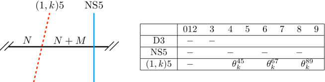
Figure 1: The type IIB brane construction of the $\text{U}(N)_{k}\times\text{U}(N)_{-k}$ ABJ theory. Here $(1,k)5$-brane, the bound state of an NS5-brane stretched in $012468$-directions and $k$ D5-branes stretched in $012579$-directions, is stretched in $012$-directions and in the three directions on $45$, $67$, $89$ planes with an angle $\theta_{k}=\arctan k$ from $4,6,8$-axes [161, 162].

The brane construction is useful in understanding the dualities (3.16) and (4.2) used in later analysis.

We can add a supersymmetric mass terms to this theory by introducing non-dynamical background vectormultiplets for the R-symmetry which are frozen to the sypersymmetric configuration $V^{\text{bgd}}=(A^{\text{bgd}}_{\mu},\sigma^{\text{bgd}},\lambda^{\text{bgd}},D^{\text{bgd}})=(0,\delta,0,-\delta)$. We can turn on three mass parameteres $(\delta_{1},\delta_{2}+\delta_{3},\delta_{2}-\delta_{3})$ corresponding to the Cartans of $\text{U}(1)\times\text{SU}(2)_{1}\times\text{SU}(2)_{2}\subset\text{SO}(6)_{R}$ under which the $(X^{1},X^{2})$ and $(Y_{1},Y_{2})$ transform respectively as $(+1,\bm{2},\bm{1})$ and $(-1,\bm{1},\bm{2})$. This gives the following masses to the chiral multiplets:

$$X^{1}:\delta_{1}+\delta_{2}+\delta_{3},\quad X^{2}:\delta_{1}-\delta_{2}-\delta_{3},\quad Y_{1}:-\delta_{1}+\delta_{2}-\delta_{3},\quad Y_{2}:-\delta_{1}-\delta_{2}+\delta_{3}.$$ (2.1)

In this paper we consider the two-parameter mass deformation with

$$\delta_{1}=\frac{m_{1}-m_{2}}{2\pi},\quad\delta_{2}=\frac{m_{1}+m_{2}}{2\pi},\quad\delta_{3}=0.$$ (2.2)

The partition function of the mass deformed ABJM theory on the three sphere is given by the supersymmetry localization formula [22], which simplifies for this choice as

$$Z_{k,M}(N,m_{1},m_{2})=\frac{(-1)^{MN+\frac{M(M-1)}{2}}e^{\frac{NM(m_{1}+m_{2})}{2}}}{N!(N+M)!}\int\frac{d^{N}x}{(2\pi)^{N}}\frac{d^{N+M}y}{(2\pi)^{N+M}}e^{\frac{ik}{4\pi}(\sum_{i=1}^{N}x_{i}^{2}-\sum_{i=1}^{N+M}y_{i}^{2})}$$

$$\quad\times\frac{\prod_{i<j}^{N}(2\sinh\frac{x_{i}-x_{j}}{2})^{2}\prod_{i<j}^{N+M}(2\sinh\frac{y_{i}-y_{j}}{2})^{2}}{\prod_{i=1}^{N}\prod_{j=1}^{N+M}(2\cosh\frac{x_{i}-y_{j}-m_{1}}{2})(2\cosh\frac{y_{i}-x_{j}-m_{2}}{2})}.$$ (2.3)

Here we have chosen the overall factor $(-1)^{MN+\frac{M(M-1)}{2}}e^{\frac{NM(m_{1}+m_{2})}{2}}$ to be the same as in [149]. Note that the partition function at $M=0$ obeys various symmetries

$$Z_{k,0}(N,m_{1},m_{2})=Z_{k,0}(N,m_{1},-m_{2}),\quad Z_{k,0}(N,m_{1},m_{2})=Z_{k,0}(N,m_{2},m_{1}),$$

$$(Z_{k,0}(N,m_{1}^{*},m_{2}^{*}))^{*}=Z_{k,0}(N,m_{1},m_{2}),$$ (2.4)

which are obvious from (2.3).

3 Bilinear relations of partition functions

In the following we review the result of [149] where it was found that the grand canonical partition function of the mass deformed ABJM theory

$$\Xi_{k,M}(\kappa;m_{1},m_{2})=\sum_{N=0}^{\infty}\kappa^{N}Z_{k,M}(N,m_{1},m_{2})$$ (3.1)

satisfies bilinear relations (3.11) for $m_{1}=m_{2}$, and display their generalizations for $m_{1}\neq m_{2}$ (3.12).

In [149] it was found that the partition function (2.3) can be rewritten in the Fermi gas formalism

$$Z_{k,M}(N,m_{1},m_{2})=\frac{Z_{k,M}(0)}{N!}\int\frac{d^{N}x}{(2\pi)^{N}}\text{det}\langle x_{i}|{\hat{\rho}}|x_{j}\rangle,$$ (3.2)

where $Z_{k,M}(0)$ is the partition function of $\text{U}(M)_{k}$ pure Chern-Simons theory (A.1) and ${\hat{\rho}}$ is the following operator of one-dimensional quantum mechanics

$${\hat{\rho}}=(-1)^{M}e^{\frac{M(m_{1}+m_{2})}{2}}\frac{e^{-\frac{im_{2}{\hat{x}}}{2\pi}}}{2\cosh\frac{{\hat{x}}+\pi iM}{2}}\biggl{(}\prod_{r=1}^{M}\frac{2\sinh\frac{{\hat{x}}-t_{M,r}}{2k}}{2\cosh\frac{{\hat{x}}-t_{M,r}-m_{1}k}{2k}}\biggr{)}\frac{e^{-\frac{im_{1}{\hat{p}}}{2\pi}}}{2\cosh\frac{{\hat{p}}}{2}}$$ (3.3)

with $t_{M,r}=2\pi i(\frac{M+1}{2}-r)$. Here we have introduced position/momentum operator ${\hat{x}},{\hat{p}}$ satisfying $[{\hat{x}},{\hat{p}}]=2\pi ik$ and the position eigenstate $|\cdot\rangle$. By using quantum dilogarithm $\Phi_{b}(z)$ [121]

$$\Phi_{b}(z)=\frac{(-e^{2\pi bz+\pi ib^{2}};e^{2\pi ib^{2}})_{\infty}}{(-e^{2\pi ib^{-1}z-\pi ib^{-2}};e^{-2\pi ib^{-2}})_{\infty}},$$ (3.4)

with $b=\sqrt{k}$, which satisfy the following relations

$$\frac{\Phi_{b}(z+ib)}{\Phi_{b}(z)}=\frac{1}{1+e^{\pi ib^{2}}e^{2\pi bz}},\quad\frac{\Phi_{b}(z+ib^{-1})}{\Phi_{b}(z)}=\frac{1}{1+e^{-\pi ib^{-2}}e^{2\pi b^{-1}z}},$$ (3.5)

we can express ${\hat{\rho}}$ as

$${\hat{\rho}}=(-1)^{M}e^{-\frac{\pi iM}{2}}e^{\frac{Mm_{2}}{2}}e^{(\frac{1}{2}-\frac{im_{2}}{2\pi}){\hat{x}}}\frac{\Phi(\frac{{\hat{x}}}{2\pi b}+\frac{ib}{2}-\frac{iM}{2b})}{\Phi(\frac{{\hat{x}}}{2\pi b}-\frac{ib}{2}+\frac{iM}{2b})}e^{-\frac{im_{1}}{2\pi}{\hat{p}}}\frac{\Phi(\frac{{\hat{x}}}{2\pi b}+\frac{iM}{2b})}{\Phi(\frac{{\hat{x}}}{2\pi b}-\frac{iM}{2b})}\frac{1}{2\cosh\frac{{\hat{p}}}{2}}.$$ (3.6)

By using the first identity of quantum dilogarithm in (3.5), we find that the inverse of ${\hat{\rho}}$ is written, up to a similarity transformation which does not affect the partition functions (3.2), as a Laurent polynomial of $e^{\frac{{\hat{x}}}{2}},e^{\frac{{\hat{p}}}{2}},e^{\frac{im_{2}{\hat{x}}}{2\pi}},e^{\frac{im_{1}{\hat{p}}}{2\pi}}$, which reads

$${\hat{\rho}}^{-1}={\hat{U}}^{-1}({\hat{\rho}}^{\prime})^{-1}{\hat{U}},\quad{\hat{U}}=\frac{\Phi_{b}(\frac{{\hat{x}}}{2\pi b}-\frac{ib}{2}+\frac{iM}{2b})}{\Phi_{b}(\frac{{\hat{x}}}{2\pi b}+\frac{ib}{2}-\frac{iM}{2b})}e^{(-\frac{1}{2}+\frac{im_{2}}{2\pi}){\hat{x}}},$$ (3.7)

with

$$({\hat{\rho}}^{\prime})^{-1}=e^{-\frac{\pi ik}{4}+(\frac{k}{4}-M)(m_{1}+m_{2})+\frac{im_{1}m_{2}k}{4\pi}}(e^{(1+\frac{i(m_{1}+m_{2})}{2\pi}){\hat{x}}^{\prime}+\frac{i(m_{1}-m_{2}){\hat{p}}^{\prime}}{2\pi}}+e^{(\frac{i(m_{1}+m_{2})}{2\pi}){\hat{x}}^{\prime}+(-1+\frac{i(m_{1}-m_{2})}{2\pi}){\hat{p}}^{\prime}}$$

$$\quad+e^{\frac{i(m_{1}+m_{2})}{2\pi}{\hat{x}}^{\prime}+(1+\frac{i(m_{1}-m_{2})}{2\pi}){\hat{p}}^{\prime}}+e^{\pi i(k-2M)}e^{(-1+\frac{i(m_{1}+m_{2})}{2\pi}){\hat{x}}^{\prime}+\frac{i(m_{1}-m_{2}){\hat{p}}^{\prime}}{2\pi}}).$$ (3.8)

Here we have redefined the canonical position/momentum operators

$${\hat{x}}^{\prime}=\frac{{\hat{x}}+{\hat{p}}}{2}-\frac{3\pi iM}{2}+\frac{\pi ik}{2}-\frac{k(m_{1}+m_{2})}{4},\quad{\hat{p}}^{\prime}=\frac{-{\hat{x}}+{\hat{p}}}{2}-\frac{\pi iM}{2}+\frac{k(m_{1}-m_{2})}{4},$$ (3.9)

which now satisfy $[{\hat{x}}^{\prime},{\hat{p}}^{\prime}]=\pi ik$, to simplify the relative coefficients of the Laurent polynomial.

To guess the bilinear relation satisfied by $\Xi_{k,M}(\kappa)$, in [149] we have consulted the ideas of the topological string/spectral theory (TS/ST) correspondence and the geometric engineering, where the classical curve ${\hat{\rho}}^{-1}|_{{\hat{x}}\rightarrow x,{\hat{p}}\rightarrow p}+\kappa=0$ is identified with the Seiberg-Witten curve of the five-dimensional ${\cal N}=1$ Yang-Mills theory engineered by the Calabi-Yau threefold. In particular, if we set $m_{1}=m_{2}=\frac{\pi i(2a-\nu)}{\nu}$ with $\nu,a\in\mathbb{N}$, by further redefining the canonical operators as

$${\hat{x}}^{\prime\prime}=\frac{2{\hat{x}}^{\prime}}{\nu},\quad{\hat{p}}^{\prime\prime}={\hat{p}}^{\prime}-\Bigl{(}1-\frac{2}{\nu}\Bigr{)}{\hat{x}}^{\prime},$$ (3.10)

we find that the curve ${\hat{\rho}}^{-1}|_{{\hat{x}}^{\prime\prime}\rightarrow x,{\hat{p}}^{\prime\prime}\rightarrow p}+\kappa=0$ coincides with the Seiberg-Witten curve of the $\text{SU}(\nu)$ pure Yang-Mills theory with only the $a$-th Coulomb parameter is turned on, which corresponds to $\kappa$. See figure 2.

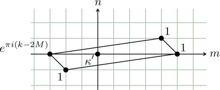
Figure 2: Newton polygon $I=\{(m,n)\}$ such that $({\hat{\rho}}^{\prime})^{-1}+\kappa\propto\sum_{(m,n)\in I}c_{mn}e^{m{\hat{x}}^{\prime\prime}+n{\hat{p}}^{\prime\prime}}$ for $m_{1}=m_{2}=\frac{\pi i(2a-\nu)}{\nu}$ with $(\nu,a)=(8,3)$. We have also displayed the coefficient $c_{mn}$ associated with each point, where $\kappa^{\prime}=e^{\frac{\pi ik}{4}-(\frac{k}{4}-M)(m_{1}+m_{2})-\frac{im_{1}m_{2}k}{4\pi}}$.

The TS/ST correspondence suggests that the grand partition function $\Xi_{k,M}(\kappa,m_{1},m_{1})$ is identified with the Nekrasov-Okounkov partition function of this theory on the self-dual $\Omega$ background $\epsilon_{1}=-\epsilon_{2}$, which is known to satisfy the $\mathfrak{q}$-discrete $\text{SU}(\nu)$ Toda bilinear equations with respect to the instanton counting parameter $z$ [164]. Since $z$ is identified with the moduli of the curve as $z=e^{-\pi i\nu(1-\frac{2M}{k})}$ [126], this fact implies that $\Xi_{k,M}(\kappa,m_{1},m_{2})$ also satisfies bilinear difference relations with respect to the shift of $M$. Indeed, by using the exact expressions of $Z_{k,M}(N,m_{1},m_{2})$ for various $k\in\mathbb{N}$, $N\in\mathbb{Z}_{\geq 0}$, $M\in\{0,1,\cdots,k\}$ as functions of $m_{1},m_{2}$ obtained by the open string formalism [53] it was found that $\Xi_{k,M}(\kappa,m_{1},m_{1})$ satisfy the following relations [149]

$$\Xi_{k,M+1}(-e^{-m_{1}}\kappa;m_{1},m_{1})\Xi_{k,M-1}(-e^{m_{1}}\kappa;m_{1},m_{1})+e^{-\frac{2\pi iM}{k}}\Xi_{k,M}(\kappa;m_{1},m_{1})^{2}$$

$$\quad-\Xi_{k,M}(-e^{-m_{1}}\kappa;m_{1},m_{1})\Xi_{k,M}(-e^{m_{1}}\kappa;m_{1},m_{1})=0.$$ (3.11)

Note that although the above argument through the five-dimensional gauge theory is valid only for $m_{1}=m_{2}=\frac{\pi i(2a-\nu)}{\nu}$, the exact expressions for $Z_{k,M}(N,m_{1},m_{2})$ tell us that (3.11) is satisfied for any complex values of $m_{1}=m_{2}$ with $|\text{Im}[m_{1}]|<\pi$. Indeed, since the partition function $Z_{k,M}(N,m_{1},m_{2})$ is holomorphic functions of $m_{1},m_{2}$ in $|\text{Im}[m_{1}]|,|\text{Im}[m_{2}]|<\pi$ for any finite $k,M,N$, if (3.11) is satisfied for any $(\nu,a)$ it follows that (3.11) is satisfied for any complex value of $m_{1}=m_{2}$ with $|\text{Im}[m_{1}]|<\pi$. Furthermore, with the exact expressions for $Z_{k,M}(N,m_{1},m_{2})$ at hand it is not difficult to find that $\Xi_{k,M}(\kappa,m_{1},m_{2})$ satisfies the following bilinear relations even for $m_{1}\neq m_{2}$:

$$\Xi_{k,M+1}(-e^{-\frac{m_{1}+m_{2}}{2}}\kappa;m_{1},m_{2})\Xi_{k,M-1}(-e^{\frac{m_{1}+m_{2}}{2}}\kappa;m_{1},m_{2})$$

$$\quad+e^{-\frac{2\pi iM}{k}}\Xi_{k,M}(e^{\frac{m_{1}-m_{2}}{2}}\kappa;m_{1},m_{2})\Xi_{k,M}(e^{-\frac{m_{1}-m_{2}}{2}}\kappa;m_{1},m_{2})$$

$$\quad-\Xi_{k,M}(-e^{-\frac{m_{1}+m_{2}}{2}}\kappa;m_{1},m_{2})\Xi_{k,M}(-e^{\frac{m_{1}+m_{2}}{2}}\kappa;m_{1},m_{2})=0.$$ (3.12)

In appendix B we explain how we have guessed this relation by using the first a few exact values of the partition function. We have checked against the exact values of $Z_{k,M}(N;m_{1},m_{2})$ that this equation is satisfied for $1\leq M\leq k-1$ for $k=2$ to the order $\kappa^{7}$, for $k=3$ to the order $\kappa^{6}$, for $k=4$ to the order $\kappa^{6}$, for $k=5$ to the order $\kappa^{5}$ and for $k=6$ to the order $\kappa^{5}$. In appendix A we list part of these exact values with which the reader can perform the same test. See [149] for the detail of the method to generate these data.

Lastly let us comment on the compatibility of the bilinear relations (3.12) with the Seiberg-like duality

$$\text{U}(N)_{k}\times\text{U}(N+M)_{-k}\longleftrightarrow\text{U}(N)_{-k}\times\text{U}(N+k-M)_{k}$$ (3.13)

which relates $Z_{k,M}(N,m_{1},m_{2})$ and $Z_{k,k-M}(N,m_{1},m_{2})$. When $m_{1}=m_{2}=0$, the duality can be understood as the Hanany-Witten effect in the type IIB brane construction [160] displayed in figure 3.

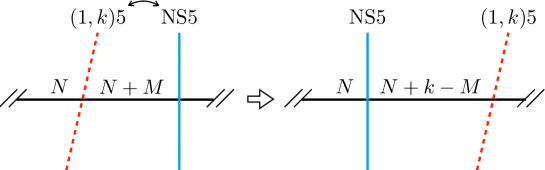
Figure 3: Hanany-Witten transition associated with the duality (3.13).

The relation between the partition function with relative ranks $M$ and $k-M$ can be proved explicitly by using the following integration identity [151, 154]

$$\frac{1}{N!}\int\frac{d^{N}z}{(2\pi)^{N}}{\cal Z}_{0,\xi}(N_{L},N;x,z){\cal Z}_{k,\eta}(N,N_{R};z,y)$$

$$=\begin{cases}\displaystyle e^{\pi i(-\frac{1}{6}-\frac{k^{2}}{12}+\frac{k(N+{\tilde{N}})}{4}+\frac{(N-{\tilde{N}})^{2}}{4}-(\xi-\zeta)^{2})}\frac{1}{{\tilde{N}}!}\int\frac{d^{\tilde{N}}z}{(2\pi)^{\tilde{N}}}{\cal Z}_{k,\eta}(N_{L},{\tilde{N}};x,{\tilde{z}}){\cal Z}_{k,\xi}({\tilde{N}},N_{R};{\tilde{z}},y)&\quad({\tilde{N}}\geq 0)\\ \displaystyle 0&\quad({\tilde{N}}<0)\end{cases},$$ (3.14)

where ${\tilde{N}}=N_{L}+N_{R}-N+k$ and

$${\cal Z}_{k,\zeta}(N_{1},N_{2};x,y)=e^{\frac{ik}{4\pi}(\sum_{i=1}^{N_{1}}x_{i}^{2}-\sum_{i=1}^{N_{2}}y_{i}^{2})}e^{-i\zeta(\sum_{i=1}^{N_{1}}x_{i}-\sum_{i=1}^{N_{2}}y_{i})}\frac{\prod_{i<j}^{N_{1}}2\sinh\frac{x_{i}-x_{j}}{2}\prod_{i<j}^{N_{2}}2\sinh\frac{y_{i}-y_{j}}{2}}{\prod_{i=1}^{N_{1}}\prod_{j=1}^{N_{2}}2\cosh\frac{x_{i}-y_{j}}{2}}.$$ (3.15)

By using this formula, we find the following relation for the partition function (2.3) with $m_{1},m_{2}\neq 0$

$$Z_{k,M}(N,m_{1},m_{2})=e^{\pi i(\frac{kN}{2}+\frac{k^{2}}{12}-\frac{k}{2}+\frac{1}{6})}e^{\frac{N(2M-k)(m_{1}+m_{2})}{2}-\frac{ikNm_{1}m_{2}}{2\pi}}(Z_{k,k-M}(N,m_{2}^{*},m_{1}^{*}))^{*},$$ (3.16)

or

$$\Xi_{k,M}(\kappa;m_{1},m_{2})=e^{\pi i(\frac{k^{2}}{12}-\frac{k}{2}+\frac{1}{6})}(\Xi_{k,k-M}(e^{-\frac{\pi ik}{2}}e^{\frac{(2M-k)(m_{1}^{*}+m_{2}^{*})}{2}+\frac{ikm_{1}^{*}m_{2}^{*}}{2\pi}}\kappa^{*};m_{2}^{*},m_{1}^{*}))^{*}$$ (3.17)

in terms of the grand partition function. Here the complex conjugation is necessary to take care of the change of the Chern-Simons levels $(k,-k)\rightarrow(-k,k)$. We see that the bilinear relations (3.12) are manifestly compatible with the Seiberg-like duality (3.17).

4 Recursion equations in $N$

In the previous section we have found that the grand partition function $\Xi_{k,M}(\kappa)$ with $0\leq M\leq k$ satisfies $k-1$ bilinear relations (3.12) which are second-order difference relations (3.12) with respect to $M$. Conversely, if we assume (3.12) to hold, it allows us to determine $\Xi_{k,M}(\kappa)$ for $2\leq M\leq k$ completely algebraically once $\Xi_{k,0}(\kappa)$ and $\Xi_{k,1}(\kappa)$ are given as initial data. Expanding (3.12) in $\kappa$, on the other hand, we can view them as an infinite set of relation among $\{Z_{k,M}(0)\}_{M=0}^{k}$, $\{Z_{k,M}(1)\}_{M=0}^{k}$, $\{Z_{k,M}(2)\}_{M=0}^{k}$ and so forth. However, these relations alone cannot be solved recursively in $N$ since the number of unknowns (which is $k+1$) at each step is larger than the number of equations at each order in $\kappa$ (which is $k-1$). In the following we see that (3.12) combined with an additional constraint from the duality cascade [154] is solvable in $N$ recursively.

To explain the constraint, let us consider the Hanany-Witten brane exchange (see figure 3) for the case with $M\geq k$. Since $k-M\leq 0$, the smallest rank also changes as $N\rightarrow N+k-M$. When $N<M-k$ we encounter a negative rank, which is interpreted that the configuration does not preserve the supersymmetry [160]. Hence the brane configurations suggest the following relation among the partition functions

$$Z_{k,M}(N)\sim\begin{cases}Z_{k,M-k}(N+k-M)&(N\geq M-k)\\ 0&(N<M-k)\end{cases}.$$ (4.1)

These relations were proved explicitly in [154] for $m_{1}=m_{2}=0$ together with the precise overall factor for $N\geq M-k$ by using the identities (3.14), which can be generalized to $m_{1},m_{2}\neq 0$ straightforwardly. As a result we find

$$Z_{k,M}(N,m_{1},m_{2})$$

$$=\begin{cases}e^{\pi i(\frac{kN}{2}+\frac{k^{2}}{12}-\frac{k}{2}+\frac{1}{6})}e^{\frac{(Nk+(M-k)^{2})(m_{1}+m_{2})}{2}-\frac{ikNm_{1}m_{2}}{2\pi}}Z_{k,M-k}(N-(M-k),m_{1},m_{2})&\quad(N\geq M-k)\\ 0&\quad(N<M-k)\end{cases}$$ (4.2)

for $M\geq k$. In particular, the grand partition functions at $M=k$ and $M=k+1$ are related to $\Xi_{k,0}(\kappa,m_{1},m_{2})$ and $\Xi_{k,1}(\kappa,m_{1},m_{2})$ as

$$\Xi_{k,k}(\kappa,m_{1},m_{2})=e^{\pi i(\frac{k^{2}}{12}-\frac{k}{2}+\frac{1}{6})}\Xi_{k,0}(e^{\frac{\pi ik}{2}}e^{\frac{k(m_{1}+m_{2})}{2}-\frac{ikm_{1}m_{2}}{2\pi}}\kappa,m_{1},m_{2}),$$ (4.3)

$$\Xi_{k,k+1}(\kappa,m_{1},m_{2})=e^{\pi i(\frac{k^{2}}{12}+\frac{1}{6})}e^{\frac{(k+1)(m_{1}+m_{2})}{2}-\frac{ikm_{1}m_{2}}{2\pi}}\kappa\Xi_{k,1}(e^{\frac{\pi ik}{2}}e^{\frac{k(m_{1}+m_{2})}{2}-\frac{ikm_{1}m_{2}}{2\pi}}\kappa,m_{1},m_{2}).$$ (4.4)

Note that the first relation is consistent with the Seiberg-like duality (3.17) with $M=k$, taking into account the fact that the partition functions at $M=0$ is real (2.4). Furthermore, from the original definition (2.3) we have

$$Z_{k,-1}(N+1,m_{1},m_{2})=\begin{cases}e^{-\frac{(2N+1)(m_{1}+m_{2})}{2}}(Z_{k,1}(N,m_{2}^{*},m_{1}^{*}))^{*}&\quad(N\geq 0)\\ 0&\quad(N=-1)\end{cases}.$$ (4.5)

Combining this with the Seiberg-like duality (3.17) we find

$$Z_{k,-1}(N+1,m_{1},m_{2})=\begin{cases}e^{-\pi i(\frac{kN}{2}+\frac{k^{2}}{12}-\frac{k}{2}+\frac{1}{6})}e^{\frac{(-kN-1)(m_{1}+m_{2})}{2}+\frac{ikNm_{1}m_{2}}{2\pi}}Z_{k,k-1}(N,m_{1},m_{2})&\quad(N\geq 0)\\ 0&\quad(N=-1)\end{cases},$$ (4.6)

or

$$\Xi_{k,-1}(\kappa;m_{1},m_{2})=e^{-\pi i(\frac{k^{2}}{12}-\frac{k}{2}+\frac{1}{6})}e^{-\frac{m_{1}+m_{2}}{2}}\kappa\Xi_{k,k-1}(e^{-\frac{\pi ik}{2}}e^{-\frac{k(m_{1}+m_{2})}{2}+\frac{ikm_{1}m_{2}}{2\pi}}\kappa;m_{1},m_{2})$$ (4.7)

in terms of the grand partition function. Interestingly, we find by using the exact values of $Z_{k,M}(N,m_{1},m_{2})$ that the bilinear relation (3.12) at $M=0$ with $\Xi_{k,-1}(\kappa;m_{1},m_{2})$ substituted with (4.7),

$$-e^{-\pi i(\frac{k^{2}}{12}-\frac{k}{2}+\frac{1}{6})}\kappa\Xi_{k,1}(-e^{-\frac{m_{1}+m_{2}}{2}}\kappa;m_{1},m_{2})\Xi_{k,k-1}(-e^{-\frac{\pi ik}{2}}e^{-\frac{(k-1)(m_{1}+m_{2})}{2}+\frac{ikm_{1}m_{2}}{2\pi}}\kappa;m_{1},m_{2})$$

$$\quad+\Xi_{k,0}(e^{\frac{m_{1}-m_{2}}{2}}\kappa;m_{1},m_{2})\Xi_{k,0}(e^{-\frac{m_{1}-m_{2}}{2}}\kappa;m_{1},m_{2})-\Xi_{k,0}(-e^{-\frac{m_{1}+m_{2}}{2}}\kappa;m_{1},m_{2})\Xi_{k,0}(-e^{\frac{m_{1}+m_{2}}{2}}\kappa;m_{1},m_{2})=0,$$ (4.8)

is also satisfied. We can also consider the bilinear relation at $M=k$ with $\Xi_{k,k}(\kappa;m_{1},m_{2})$ and $\Xi_{k,k+1}(\kappa;m_{1},m_{2})$ substituted with (4.3) and (4.4), which turns out to be identical to (4.8).

Combining this new relation with (3.12), now we have $k-1$ equations at each order in $\kappa$ against $k-1$ independent partition functions $Z_{k,M}(N)$ with $M=0,1,\cdots,k-1$. Hence we have a sufficient number of equations to solve them with respect to $N$ recursively. In particular, due to the additional $\kappa$ in the first term, (4.8) at the order $\kappa^{N}$ gives an expression of $Z_{k,0}(N,m_{1},m_{2})$ which consists only of $Z_{k,M}(N^{\prime},m_{1},m_{2})$ with $N^{\prime}<N$. Once we determine $Z_{k,0}(N)$, the other bilinear relations (3.12) at order $\kappa^{N}$ are linear equations for $(Z_{k,1}(N),\cdots,Z_{k,k-1}(N))$ which can be inverted straightforwardly. Hence the recursive procedure schematically goes as follows

$$\begin{pmatrix}\text{input: }\\ \{Z_{k,M}(0)\}_{M=0}^{k-1}\end{pmatrix}$$

$$\rightarrow\begin{pmatrix}Z_{k,0}(1)\text{ from }\eqref{qTodam1neqm2atedge1}\\ \downarrow\\ \{Z_{k,M}(1)\}_{M=1}^{k-1}\text{ from }\eqref{qTodam1neqm2}\end{pmatrix}\rightarrow\begin{pmatrix}Z_{k,0}(2)\text{ from }\eqref{qTodam1neqm2atedge1}\\ \downarrow\\ \{Z_{k,M}(2)\}_{M=1}^{k-1}\text{ from }\eqref{qTodam1neqm2}\end{pmatrix}\rightarrow\begin{pmatrix}Z_{k,0}(3)\text{ from }\eqref{qTodam1neqm2atedge1}\\ \downarrow\\ \{Z_{k,M}(3)\}_{M=1}^{k-1}\text{ from }\eqref{qTodam1neqm2}\end{pmatrix}\rightarrow\cdots.$$ (4.9)

In the following subsections we display the recursive relations more explicitly for $k=1$ and $k\geq 2$.

4.1 $k=1$

For $k=1$ we have only one independent grand partition function $\Xi_{k,0}(\kappa;m_{1},m_{2})$, with which $\Xi_{k,1}(\kappa;m_{1},m_{2})$ and $\Xi_{k,2}(\kappa;m_{1},m_{2})$ are written as

$$\Xi_{1,1}(\kappa;m_{1},m_{2})=e^{-\frac{\pi i}{4}}\Xi_{1,0}(ie^{\frac{m_{1}+m_{2}}{2}-\frac{im_{1}m_{2}}{2\pi}}\kappa;m_{1},m_{2}),$$

$$\Xi_{1,2}(\kappa;m_{1},m_{2})=e^{m_{1}+m_{2}-\frac{im_{1}m_{2}}{2\pi}}\kappa\Xi_{1,0}(-e^{m_{1}+m_{2}-\frac{im_{1}m_{2}}{\pi}}\kappa;m_{1},m_{2}).$$ (4.10)

Here we have used the symmetry properties (2.4) of $Z_{k,0}(N,m_{1},m_{2})$ to simpilfy the right-hand sides. The bilinear relation used for the recursive approach (4.9) consist only of (4.8):

$$\Xi_{1,0}(e^{\frac{m_{1}-m_{2}}{2}}\kappa;m_{1},m_{2})\Xi_{1,0}(e^{-\frac{m_{1}-m_{2}}{2}}\kappa;m_{1},m_{2})-\Xi_{1,0}(-e^{\frac{m_{1}+m_{2}}{2}}\kappa;m_{1},m_{2})\Xi_{1,0}(-e^{-\frac{m_{1}+m_{2}}{2}}\kappa;m_{1},m_{2})$$

$$\quad-\kappa\Xi_{1,0}(-ie^{-\frac{im_{1}m_{2}}{2\pi}}\kappa;m_{1},m_{2})\Xi_{1,0}(ie^{\frac{im_{1}m_{2}}{2\pi}}\kappa;m_{1},m_{2})=0.$$ (4.11)

By solving the bilinear relation at order $\kappa^{N}$ for $Z_{1,0}(N;m_{1},m_{2})$, we find

$$Z_{0}(N;m_{1},m_{2}) =\frac{1}{H_{1,0,N}}\Bigl{[}\sum_{n=0}^{N-1}R^{2n-N+1}Z_{1,0}(n;m_{1},m_{2})Z_{1,0}(N-1-n;m_{1},m_{2})$$

$$\quad\quad-\sum_{n=1}^{N-1}I_{1,0,2n-N}Z_{1,0}(n;m_{1},m_{2})Z_{1,0}(N-n;m_{1},m_{2})\Bigr{]},$$ (4.12)

where

$$H_{k,\ell,n}=2\cosh\frac{(m_{1}-m_{2})n}{2}-e^{\frac{2\pi i\ell}{k}}(-1)^{n}2\cosh\frac{(m_{1}+m_{2})n}{2},\quad I_{k,\ell,n}=e^{\frac{(m_{1}-m_{2})n}{2}}-e^{\frac{2\pi i\ell}{k}}(-1)^{n}e^{\frac{(m_{1}+m_{2})n}{2}},$$

$$R=ie^{\frac{im_{1}m_{2}}{2\pi}}.$$ (4.13)

We will use the same symbols $H_{k,\ell,n},I_{k,\ell,n},R$ also for $k\geq 2$. Note that to obtain (4.12) we have used the fact that $Z_{1,0}(0;m_{1},m_{2})=1$.

From (4.12) we find that the partition functions are expanded as

$$Z_{1,0}(N;m_{1},m_{2})=\sum_{a=-L_{N}}^{L_{N}}R^{a}f_{a}(N),\quad L_{N}=\frac{N(N-1)}{2}.$$ (4.14)

Here $f_{a}(N)$ are some rational functions of $e^{\frac{m_{1}}{2}}$ and $e^{\frac{m_{2}}{2}}$ which are determined by the recursion relation (4.12) with the initial condition $f_{0}(0)=1$. Note also that since $Z_{1,0}(N;m_{1},m_{2})$ are real functions of $m_{1},m_{2}$ and $f_{a}(N)$ are realt functions of $m_{1},m_{2}$ (which is obvious from (4.12)), $f_{a}(N)$ satisfy the following relation

$$f_{-a}(N)=f_{a}(N).$$ (4.15)

4.2 $k\geq 2$

To write down the recursion relation for $k\geq 2$, it is convenient to redefine the partition function $Z_{k,M}(N)$ and the grand partition functions $\Xi_{k,M}(\kappa)$ with $M\geq 1$ as

$$Z_{k,M}^{\prime}(N)=e^{\pi i(\frac{M^{3}}{3k}+\frac{M^{2}}{2}+(-\frac{11k}{12}+\frac{1}{2}-\frac{1}{6k})M)}\Bigl{(}-e^{-\frac{(m_{1}+m_{2})}{2}}\Bigr{)}^{MN}Z_{k,M}(N),$$

$$\Xi_{k,M}^{\prime}(\kappa)=\sum_{N=0}^{\infty}\kappa^{N}Z_{k,M}^{\prime}(N)=e^{\pi i(\frac{M^{3}}{3k}+\frac{M^{2}}{2}+(-\frac{11k}{12}+\frac{1}{2}-\frac{1}{6k})M)}\Xi_{k,M}\Bigl{(}\Bigl{(}-e^{-\frac{(m_{1}+m_{2})}{2}}\Bigr{)}^{M}\kappa\Bigr{)},$$ (4.16)

With this redefinition, the bilinear relations (3.12),(4.8) are written as ($M=1,\cdots,k-2$)

$$\kappa\Xi_{k,1}^{\prime}(\kappa;m_{1},m_{2})\Xi_{k,k-1}^{\prime}(R^{k}\kappa;m_{1},m_{2})-\prod_{\pm}\Xi^{\prime}_{k,0}(e^{\pm\frac{m_{1}-m_{2}}{2}}\kappa;m_{1},m_{2})$$

$$\quad\quad+\prod_{\pm}\Xi^{\prime}_{k,0}(-e^{\mp\frac{m_{1}+m_{2}}{2}}\kappa;m_{1},m_{2})=0,$$

$$\prod_{\pm}\Xi^{\prime}_{k,M\pm 1}(\kappa;m_{1},m_{2})-\prod_{\pm}\Xi^{\prime}_{k,M}(e^{\pm\frac{m_{1}-m_{2}}{2}}\kappa;m_{1},m_{2})+e^{\frac{2\pi iM}{k}}\prod_{\pm}\Xi^{\prime}_{k,M}(-e^{\mp\frac{m_{1}+m_{2}}{2}}\kappa;m_{1},m_{2})=0,$$

$$\Xi^{\prime}_{k,0}(R^{-k}\kappa;m_{1},m_{2})\Xi^{\prime}_{k,k-2}(\kappa)-\prod_{\pm}\Xi^{\prime}_{k,k-1}(e^{\pm\frac{m_{1}-m_{2}}{2}}\kappa;m_{1},m_{2})+e^{\frac{2\pi i(k-1)}{k}}\prod_{\pm}\Xi^{\prime}_{k,k-1}(-e^{\mp\frac{m_{1}+m_{2}}{2}}\kappa;m_{1},m_{2})=0.$$ (4.17)

Looking at the coefficients of $\kappa^{N}$, we find

$$Z_{k,0}(N)=\frac{1}{H_{k,0,N}}\Bigl{(}\sum_{n=1}^{N-1}R^{kn}Z_{k,1}^{\prime}(N-1-n)Z_{k,k-1}^{\prime}(n)-\sum_{n=1}^{N-1}I_{k,0,2n-N}Z_{k,0}(n)Z_{k,0}(N-n)\Bigr{)}$$ (4.18)

and

$$Z_{2,1}^{\prime}(N)=\sum_{n=1}^{N-1}I_{2,1,n}Z_{2,1}^{\prime}(n)Z_{2,1}^{\prime}(N-n)-\sum_{n=0}^{N}Z_{2,0}(n)Z_{2,0}(N-n) \quad(k=2)$$

$$\begin{pmatrix}Z_{k,1}^{\prime}(N)\\ Z_{k,2}^{\prime}(N)\\ \vdots\\ \\ \\ \vdots\\ Z_{k,k-1}^{\prime}(N)\end{pmatrix}=\begin{pmatrix}b_{1}&c_{1}&0&\cdots&&&&\cdots&0\\ a_{2}&b_{2}&c_{2}&0&\cdots&&&\cdots&0\\ 0&a_{3}&b_{3}&c_{3}&0&\cdots&&\cdots&0\\ &&&&\ddots&&&&\\ 0&\cdots&&\cdots&0&a_{k-3}&b_{k-3}&c_{k-3}&0\\ 0&\cdots&&&\cdots&0&a_{k-2}&b_{k-2}&c_{k-2}\\ 0&\cdots&&&&\cdots&0&a_{k-1}&b_{k-1}\end{pmatrix}^{-1}\begin{pmatrix}d_{1}\\ d_{2}\\ \vdots\\ \\ \\ \vdots\\ d_{k-1}\end{pmatrix} \quad(k\geq 3),$$ (4.19)

where

$$a_{M}=Z_{k,M+1}^{\prime}(0),\quad b_{M}=-H_{k,M,N}Z_{M}^{\prime}(0),\quad c_{M}=Z_{k,M-1}^{\prime}(0),$$

$$d_{1}=\sum_{n=1}^{N-1}I_{k,1,n}Z_{k,1}^{\prime}(n)Z_{k,1}^{\prime}(N-n)-\sum_{n=0}^{N-1}Z_{k,2}^{\prime}(n)Z_{k,0}^{\prime}(N-n),$$

$$d_{M}=\sum_{n=1}^{N-1}I_{k,M,n}Z_{k,M}^{\prime}(n)Z_{k,M}^{\prime}(N-n)-\sum_{n=1}^{N-1}Z_{k,2}^{\prime}(n)Z_{k,0}^{\prime}(N-n)\quad(M=2,\cdots,k-2),$$

$$d_{k-1}=\sum_{n=1}^{N-1}I_{k,k-1,n}Z_{k,k-1}^{\prime}(n)Z_{k,k-1}^{\prime}(N-n)-\sum_{n=1}^{N}Z_{k,0}^{\prime}(n)Z_{k,k-2}^{\prime}(N-n),$$ (4.20)

with $Z_{k,0}^{\prime}(N)=Z_{k,0}(N)$.

As is the case for $k=1$, the recursion relations (4.18),(4.19) tell us that the partition functions have the following structures for general $M,N$:

$$Z_{k,0}(N)=\sum_{a=-K_{N}^{(0)}}^{L_{N}^{(0)}}R^{a}f_{a}^{(0)}(N),$$

$$Z_{k,M}^{\prime}(N)=\sum_{a=-K_{N}^{(1)}}^{L_{N}^{(1)}}R^{a}f_{a}^{(M)}(N)\quad(1\leq M\leq k-1),$$ (4.21)

with $f_{a}^{(M)}(N)$ some rational functions of $e^{\frac{m_{1}}{2}}$ and $e^{\frac{m_{2}}{2}}$. The upper/lower bound of the summation index $a$ can be estimated from the recursion relation (4.18),(4.19) as

$$L_{N}^{(0)}=\text{max}\biggl{[}\mathop{\text{max}}_{0\leq n\leq N-1}(kn+L^{(1)}_{N-1-n}+L^{(1)}_{n}),\mathop{\text{max}}_{1\leq n\leq N-1}(L_{n}^{(0)}+L_{N-n}^{(0)})\biggr{]},$$

$$K_{N}^{(0)}=-\text{min}\biggl{[}\mathop{\text{min}}_{0\leq n\leq N-1}(kn-K^{(1)}_{N-1-n}-K^{(1)}_{n}),\mathop{\text{min}}_{1\leq n\leq N-1}(-K_{n}^{(0)}-K_{N-n}^{(0)})\biggr{]},$$

$$L_{N}^{(1)}=\begin{cases}\displaystyle\text{max}\biggl{[}\mathop{\text{max}}_{1\leq n\leq N-1}(L^{(1)}_{n}+L^{(1)}_{N-n}),\mathop{\text{max}}_{1\leq n\leq N}(-2n+L_{n}^{(0)}+L_{N-n}^{(0)})\biggr{]},&\quad(k=2)\vspace{0.2cm}\\ \displaystyle\text{max}\biggl{[}\mathop{\text{max}}_{1\leq n\leq N-1}(L^{(1)}_{n}+L^{(1)}_{N-n}),\mathop{\text{max}}_{0\leq n\leq N-1}(L_{n}^{(1)}+L_{N-n}^{(0)}),\mathop{\text{max}}_{1\leq n\leq N}(-kn+L_{n}^{(0)}+L_{N-n}^{(1)})\biggr{]},&\quad(k\geq 3)\end{cases},$$

$$K_{N}^{(1)}=\begin{cases}\displaystyle-\text{min}\biggl{[}\mathop{\text{min}}_{1\leq n\leq N-1}(-K^{(1)}_{n}-K^{(1)}_{N-n}),\mathop{\text{min}}_{1\leq n\leq N}(-2n-K_{n}^{(0)}-K_{N-n}^{(0)})\biggr{]},&\quad(k=2)\vspace{0.2cm}\\ \displaystyle-\text{min}\biggl{[}\mathop{\text{min}}_{1\leq n\leq N-1}(-K^{(1)}_{n}-K^{(1)}_{N-n}),\mathop{\text{min}}_{0\leq n\leq N-1}(-K_{n}^{(1)}-K_{N-n}^{(0)}),\mathop{\text{min}}_{1\leq n\leq N}(-kn-K_{n}^{(0)}-K_{N-n}^{(1)})\biggr{]},&\quad(k\geq 3)\end{cases},$$ (4.22)

which are solved explicitly as

$$L^{(0)}_{N}=K^{(0)}_{N}=L^{(1)}_{N}=\frac{k(N^{2}-N)}{2},\quad K^{(1)}_{N}=\frac{k(N^{2}+N)}{2}.$$ (4.23)

5 Large $N$ behavior of $Z_{k,0}(N;m_{1},m_{2})$ with $\sqrt{|m_{1}m_{2}|}\geq\pi$

The recursive approach (4.9) allows us to calculate exact values of $Z_{k,M}(N;m_{1},m_{2})$ efficiently for arbitrary values of $m_{1},m_{2}$ with $|\text{Im}[m_{1}]|<\pi,|\text{Im}[m_{2}]|<\pi$ and finite but large values of $N$, which are reliable data for studying the large $N$ expansion of the partition function. By using these data, in this section we investigate the large $N$ expansion of the partition function in the supercritical regime $\sqrt{m_{1}m_{2}}>\pi$ [106].

First let us recall the large $N$ expansion for $m_{1},m_{2}\in i\mathbb{R}$ with $|m_{1}|,|m_{2}|<\pi$ where there is no phase transition. By applying the standard WKB analysis for the Ferim gas formalism, we find [105]

$$Z_{k,0}(N;m_{1},m_{2})\approx Z_{k,0}^{\text{pert}}(N;m_{1},m_{2})=e^{A}C^{-\frac{1}{3}}\text{Ai}[C^{-\frac{1}{3}}(N-B)],$$ (5.1)

where

$$C=\frac{2}{\pi^{2}k(1+\pi^{-2}m_{1}^{2})(1+\pi^{-2}m_{2}^{2})},\quad B=\frac{2-\pi^{-2}(m_{1}^{2}+m_{2}^{2})}{6k(1+\pi^{-2}m_{1}^{2})(1+\pi^{-2}m_{2}^{2})}-\frac{k}{12}+\frac{k}{2}\Bigl{(}\frac{1}{2}-\frac{M}{k}\Bigr{)}^{2},$$

$$A=\frac{1}{4}\sum_{\pm}(A_{\text{ABJM}}((1\pm i\pi^{-1}m_{1})k)+A_{\text{ABJM}}((1\pm i\pi^{-1}m_{2})k))$$ (5.2)

with [165]v2

$$A_{\text{ABJM}}(k)=\frac{2\zeta(3)}{\pi^{2}k}\Bigl{(}1-\frac{k^{3}}{16}\Bigr{)}+\frac{k^{2}}{\pi^{2}}\int_{0}^{\infty}\frac{x\log(1-e^{-2x})}{e^{kx}-1}.$$ (5.3)

Here the cofficient $B$ for $M>0$ was guessed in [88, 94]. The Airy function (5.1) gives the leading behavior of the free energy in the large $N$ limit

$$-\log Z_{k,0}(N)=\frac{\pi\sqrt{2k(1+\pi^{-2}m_{1}^{2})(1+\pi^{-2}m_{2}^{2})}}{3}N^{\frac{3}{2}}+{\cal O}(N^{\frac{1}{2}})$$ (5.4)

together with the all order $1/N$ perturbative corrections. In [105] we found that the free energy agrees excellently with $-\log Z^{\text{pert}}_{k,0}(N)$ even for finite $N$, up to $1/N$ non-perturbative corrections. The exponential behaviors of the non-perturbative effects are of the form

$$e^{-\sum_{\omega}n_{\omega}\omega\sqrt{\frac{N-B}{C}}},\quad(n_{\omega}\in\mathbb{Z}_{\geq 0},\quad\sum_{\omega}n_{\omega}\geq 1).$$ (5.5)

The list of $\omega$’s was identified to consist (at least) of

$$\{\omega\}\supset\{\omega^{\text{MB}}_{1,+},\omega^{\text{MB}}_{1,-},\omega^{\text{MB}}_{2,+},\omega^{\text{MB}}_{2,-},1,\omega^{\text{WS}}_{+,+},\omega^{\text{WS}}_{+,-},\omega^{\text{WS}}_{-,+},\omega^{\text{WS}}_{-,-},\},$$ (5.6)

with

$$\omega^{\text{MB}}_{i,\pm}=\frac{2}{1\pm\frac{im_{i}}{\pi}},\quad\omega^{\text{WS}}_{\pm,\pm^{\prime}}=\frac{4}{k(1\pm\frac{im_{1}}{\pi})(1\pm^{\prime}\frac{im_{2}}{\pi})}.$$ (5.7)

To describe these results it is more convenient to consider the modified grand potential $J(\mu)$ defined by

$$\Xi_{k,M}(\kappa)=\sum_{N=0}^{\infty}\kappa^{N}Z_{k,M}(N)=\sum_{n\in\mathbb{Z}}e^{J(\mu+2\pi in)},$$ (5.8)

rather than the partition function $Z_{k,M}(N)$ itself, which is related to $Z_{k,M}(N)$ by the inversion formula

$$Z_{k,M}(N)=\int_{-i\infty}^{\infty}\frac{d\mu}{2\pi i}e^{J(\mu)-\mu N}.$$ (5.9)

The above-mentioned large $N$ behaviors (5.1),(5.5) of the partition function $Z_{k,M}(N)$ originate from the large $\mu$ expansion of $J(\mu)$

$$J(\mu)=J_{\text{pert}}(\mu)+J_{\text{np}}(\mu),$$ (5.10)

with

$$J_{\text{pert}}(\mu)=\frac{C}{3}\mu^{3}+B\mu+A,\quad J_{\text{np}}(\mu)=\sum_{\{n_{\omega}\}}\gamma(\{n_{\omega}\})e^{-(\sum_{\omega}n_{\omega}\omega)\mu}.$$ (5.11)

In the list of the exponents $\omega$ (5.6), the first five exponents $\omega^{\text{MB}}_{i,\pm}$ and $1$ correspond in the massless limit to the D2-instantons in the ABJM theory [30]. These instanton exponents were identified in [105] through the WKP expansion of $J(\mu)$ together with the small $k$ expansion of the instanton coefficients $\gamma(\{n_{\omega}\})$. On the other hand, the last four exponents $\omega^{\text{WS}}_{\pm,\pm^{\prime}}$ are the generalization of the F1-instantons in the ABJM theory [166], which were guessed by analyzing the deviation of the exact values of the partition function at finite $N$ ($N\lesssim 10$) from $Z_{k,M}^{\text{pert}}(N)$ (5.1). By using the numerical values of $Z_{k,M}(N)$ in high precision with $N\gtrsim 100$ obtained by the recursion relation we can confirm this guess for the worldsheet instanton exponents, and further determine the coefficient $\gamma(\{n_{\omega}\})$ of the first worldsheet instantons as

$$\gamma(n_{\omega^{\text{WS}}_{\pm,\pm^{\prime}}}=1,\text{other }n_{\omega}=0)=\frac{\cos\frac{2\pi M}{k}}{4\sin\frac{2\pi}{k(1\pm\frac{im_{1}}{\pi})}\sin\frac{2\pi}{k(1\pm^{\prime}\frac{im_{2}}{\pi})}}.$$ (5.12)

See appendix C for the comparison with the coefficient extracted from the numerical values of $Z_{k,M}(N)$. Note that the coefficients $\gamma(n^{\text{WS}}_{\pm,\pm}=1,\text{other }n_{\omega}=0)$ are consistent with the coefficients recently obtained in the gravity side for $m_{1}=m_{2}$ and at leading order in the ’t Hooft expansion [83], while for $\gamma(n^{\text{WS}}_{\pm,\mp}=1,\text{other }n_{\omega}=0)$ our results (5.12) are inconsistent with [83]. It would be interesting to extend the comparison for finite $k$ as is done in [84] for the massless case, and also to investigate the reasons for the disagreement in $\gamma(n^{\text{WS}}_{\pm,\mp}=1,\text{other }n_{\omega}=0)$.

The large $N$ expansion explained so far agrees excellently with the actual values of the partition function $Z_{k,M}(N)$ for $m_{1},m_{2}\in i\mathbb{R}$. The two results show good agreement even when $m_{1},m_{2}$ are small real numbers. However, when we apply these results for real mass parameters with $\sqrt{|m_{1}m_{2}|}>\pi$, the real parts of the instanton exponents $\omega^{\text{WS}}_{++}$ and $\omega^{\text{WS}}_{--}$ become negative. Since the corresponding non-perturbative effects are exponentially large in $N$, the $1/N$ expansion breaks down. As a result, the Airy function (5.1) may not be the correct expansion ponit in this regime of the mass parameters, which suggests that $Z_{k,M}(N)$ exhibits a large $N$ phase transition at $\sqrt{|m_{1}m_{2}|}=\pi$.

The existence of the large $N$ phase transition at $\sqrt{|m_{1}m_{2}|}=\pi$ is also supported from several different analyses. In [103, 104] the partition function was analyzed for $M=0$ and $m_{1}=m_{2}=m$ in the large $N$ limit with $k$ kept fixed by the large $N$ saddle point approximation. As a result, it was found that while the leading behavior of the large $N$ free energy $-\log Z\approx\frac{\pi\sqrt{2k}}{3}(1+\pi^{-2}m^{2})N^{\frac{3}{2}}$ is reproduced by the solution of the saddle point equations obtained by a continuous deformation of the solution at $m=0$, the solution becomes inconsistent for $|m|\geq\pi$. In [106] the partition function with $M=0$ and $m_{1}\neq m_{2}$ was studied numerically for finite $N$ and found to deviate from the expected asymptotic behavior $-\log Z_{k,0}(N)\approx\frac{\pi\sqrt{2k(1+\pi^{-2}m_{1}^{2})(1+\pi^{-2}m_{2}^{2})}}{3}N^{\frac{3}{2}}$ when $\sqrt{|m_{1}m_{2}|}\geq\pi$. In all of these analyses, however, the concrete large $N$ behavior of the partition function in the supercritical regime $\sqrt{|m_{1}m_{2}|}\geq\pi$ was elusive. In the rest of this section we try to address this problem by using the exact expressions/numerical values of $Z_{k,M}(N;m_{1},m_{2})$ obtained by the recursion relations (4.9). For simplicity, in the following we consider only $Z_{k,M}(N)$ with $M=0$.

5.1 Large mass asymptotics

Let us first recall the general structure of the partition function (4.14),(4.21) suggested by the recursion relation. Due to the factors $R^{a}=(ie^{\frac{im_{1}m_{2}}{2\pi}})^{a}$, the partition function typically oscillates rapidly with respect to $m_{1},m_{2}$, and can even crosses zero as observed in [106]. As $N$ increases, however, we observe that the partition function does not show the oscillation in $m_{1},m_{2}$ for some special values of $N$, as displayed in figure 4.

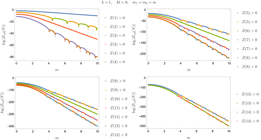
Figure 4: Oscillation of the partition functions for $k=1$, $M=0$ around $Z_{1,0}(N)=0$. For $N=1,3,6,10$ the partition function is positive definite.

To figure out the pattern, it is convenient to look at the large mass asymptotics of the partition function, which is obtained by keeping only the most dominant (namely, least suppressed in $m_{1},m_{2}$) $f_{a}(N)$’s in the summation (4.14),(4.21). For $k=1$ we find

$$Z_{1,0}(1)\rightarrow e^{-\frac{m_{1}+m_{2}}{2}},\quad Z_{1,0}(2)\rightarrow e^{-3\cdot\frac{m_{1}+m_{2}}{2}}(-R-R^{-1}),\quad Z_{1,0}(3)\rightarrow e^{-5\cdot\frac{m_{1}+m_{2}}{2}},$$

$$Z_{1,0}(4)\rightarrow e^{-8\cdot\frac{m_{1}+m_{2}}{2}}(1+R^{2}+R^{-2}),\quad Z_{1,0}(5)\rightarrow e^{-11\cdot\frac{m_{1}+m_{2}}{2}}(1+R^{2}+R^{-2}),\quad Z_{1,0}(6)\rightarrow e^{-14\cdot\frac{m_{1}+m_{2}}{2}},$$

$$Z_{1,0}(7)\rightarrow e^{-18\cdot\frac{m_{1}+m_{2}}{2}}(-R-R^{-1}-R^{3}-R^{-3}),\quad Z_{1,0}(8)\rightarrow e^{-22\cdot\frac{m_{1}+m_{2}}{2}}(2+R^{2}+R^{-2}+R^{4}+R^{-4}),$$

$$Z_{1,0}(9)\rightarrow e^{-26\cdot\frac{m_{1}+m_{2}}{2}}(-R-R^{-1}-R^{3}-R^{-3}),\quad Z_{1,0}(10)\rightarrow e^{-30\cdot\frac{m_{1}+m_{2}}{2}},$$

$$Z_{1,0}(11)\rightarrow e^{-35\cdot\frac{m_{1}+m_{2}}{2}}(1+R^{2}+R^{-2}+R^{4}+R^{-4}),$$

$$Z_{1,0}(12)\rightarrow e^{-40\cdot\frac{m_{1}+m_{2}}{2}}(1+R^{2}+R^{-2}+R^{4}+R^{-4}+R^{6}+R^{-6}),$$

$$Z_{1,0}(13)\rightarrow e^{-45\cdot\frac{m_{1}+m_{2}}{2}}(2+2R^{2}+2R^{-2}+R^{4}+R^{-4}+R^{6}+R^{-6}),$$

$$Z_{1,0}(14)\rightarrow e^{-50\cdot\frac{m_{1}+m_{2}}{2}}(1+R^{2}+R^{-2}+R^{4}+R^{-4}),\quad\cdots.$$ (5.13)

We find that the oscillation is absent when

$$N=N_{n}^{(1)}=\frac{n(n+1)}{2}\quad(n=1,2,\cdots).$$ (5.14)

We also find that the exponents of the overall asymptotic decay $Z(N)\sim e^{-\frac{\nu^{(1)}(N)(m_{1}+m_{2})}{2}}$,

$$\nu^{(1)}(1)=1,\quad\nu^{(1)}(2)=3,\quad\nu^{(1)}(3)=5,\quad\nu^{(1)}(4)=8,\quad\nu^{(1)}(5)=11,\quad\nu^{(1)}(6)=14,\quad\nu^{(1)}(7)=18,$$

$$\nu^{(1)}(8)=22,\quad\nu^{(1)}(9)=26,\quad\nu^{(1)}(10)=30,\quad\nu^{(1)}(11)=35,\quad\nu^{(1)}(12)=40,\quad\nu^{(1)}(13)=45,\quad\nu^{(1)}(14)=50,\cdots$$ (5.15)

obeys the following general formula

$$\nu^{(1)}(N)=\sum_{n=1}^{N}\Bigl{\lfloor}\frac{1}{2}+\sqrt{2n}\Bigr{\rfloor},$$ (5.16)

where $\lfloor x\rfloor$ is the largest integer which satisfy $\lfloor x\rfloor\leq x$. In particular, for $N=N_{n}^{(1)}$ (5.16) simplifies and we find

$$Z_{1,0}(N_{n}^{(1)})\rightarrow e^{-\frac{n(n+1)(2n+1)}{6}\cdot\frac{m_{1}+m_{2}}{2}}.$$ (5.17)

For $k=2$, we find

$$Z_{2,0}(1)\rightarrow e^{-\frac{m_{1}+m_{2}}{2}}\cdot\frac{1}{2},\quad Z_{2,0}(2)\rightarrow e^{-4\cdot\frac{m_{1}+m_{2}}{2}}\Bigl{(}1+\frac{R^{2}+R^{-2}}{2}\Bigr{)},\quad Z_{2,0}(3)\rightarrow e^{-7\cdot\frac{m_{1}+m_{2}}{2}}\Bigl{(}\frac{1}{2}+\frac{R^{2}+R^{-2}}{2}\Bigr{)},$$

$$Z_{2,0}(4)\rightarrow e^{-10\cdot\frac{m_{1}+m_{2}}{2}}\cdot\frac{1}{4},\quad Z_{2,0}(5)\rightarrow e^{-15\cdot\frac{m_{1}+m_{2}}{2}}\Bigl{(}\frac{1}{2}+\frac{R^{2}+R^{-2}}{2}+\frac{R^{4}+R^{-4}}{4}\Bigr{)},$$

$$Z_{2,0}(6)\rightarrow e^{-20\cdot\frac{m_{1}+m_{2}}{2}}\Bigl{(}\frac{5}{4}+R^{2}+R^{-2}+\frac{R^{4}+R^{-4}}{2}+\frac{R^{6}+R^{-6}}{4}\Bigr{)},$$

$$Z_{2,0}(7)\rightarrow e^{-25\cdot\frac{m_{1}+m_{2}}{2}}\Bigl{(}1+\frac{3(R^{2}+R^{-2})}{4}+\frac{R^{4}+R^{-4}}{2}+\frac{R^{6}+R^{-6}}{4}\Bigr{)},$$

$$Z_{2,0}(8)\rightarrow e^{-30\cdot\frac{m_{1}+m_{2}}{2}}\Bigl{(}\frac{1}{4}+\frac{R^{2}+R^{-2}}{4}+\frac{R^{4}+R^{-4}}{4}\Bigr{)},\quad Z_{2,0}(9)\rightarrow e^{-35\cdot\frac{m_{1}+m_{2}}{2}}\cdot\frac{1}{8},\quad\cdots.$$ (5.18)

We observe $Z_{2,0}(N)\sim e^{-\nu^{(2)}(N)\cdot\frac{m_{1}+m_{2}}{2}}$ with

$$\nu^{(2)}(N)=\sum_{n=1}^{N}(1+2\lfloor\sqrt{n-1}\rfloor).$$ (5.19)

We also observe that the large mass asymptotics of the partition function does not oscillate when $N=N_{n}^{(2)}$ with

$$N_{n}^{(2)}=n^{2}.$$ (5.20)

Again $\nu^{(2)}(N)$ (5.19) simplifies for these special values of $N$. Taking into account also the overall constant we find that $Z_{2,0}(N_{n}^{(2)})$ has the following simple large mass asymptotics:

$$Z_{2,0}(N_{n}^{(2)})\rightarrow 2^{-n}e^{-\frac{n(4n^{2}-1)}{3}\cdot\frac{m_{1}+m_{2}}{2}}.$$ (5.21)

As $k$ increases, the analytic expression for $Z_{k,0}(N)$ becomes more lengthy even at relatively small $N$, for which it is difficult to continue the same analysis as $k=1,2$. Nevertheless, we can study the behavior of the partition funtion at higher $N$ by solving the recursion relation (4.18),(4.19) numerically with high precision. For example, for $m_{1}=m_{2}=5$ we can reach the partition function for $k=3,M=0$ with $N=341$ by choosing the initial precision as $20000$ digits. As a result we find that there is an infinite sequence of $N$’s, which we shall call $N^{(3)}_{n}$, for which the partition function $Z_{3,0}(N^{(3)}_{n})$ does not oscillate around zero. Once we identify $N^{(3)}_{n}$ we can further study the large mass asymptotics of $Z_{3,0}(N^{(3)}_{n})$, finding a simple formula analogous to (5.17),(5.21) for $k=1,2$. The same analysis can be repeated also for $k=4$. In table 1 we summarize the list of $N_{n}^{(k)}$ and the large mass asymptotics of $Z_{k,0}(N^{(k)}_{n})$.

$k$	$N^{(k)}_{n}$	$Z_{k,0}^{\text{asym}}(N_{n}^{(k)})$
$1$	$\frac{n(n+1)}{2}$	$e^{-\frac{n(n+1)(2n+1)}{6}\cdot\frac{m_{1}+m_{2}}{2}}$
$2$	$n^{2}$	$2^{-n}e^{-\frac{n(4n^{2}-1)}{3}\cdot\frac{m_{1}+m_{2}}{2}}$
		$3^{-\frac{n+3}{3}}e^{-(\frac{n^{3}}{9}+\frac{n^{2}}{2}+\frac{7n}{6}+1)\cdot\frac{m_{1}+m_{2}}{2}}\,\,(n\equiv 0\text{ mod }3)$
$3$	$\left\lceil\frac{(n+1)(n+2)}{6}\right\rceil$	$3^{-\frac{n+2}{3}}e^{-(\frac{n^{3}}{9}+\frac{n^{2}}{2}+\frac{n}{2}-\frac{1}{9})\cdot\frac{m_{1}+m_{2}}{2}}\,\,(n\equiv 1\text{ mod }3)$
		$3^{-\frac{n+1}{3}}e^{-(\frac{n^{3}}{9}+\frac{n^{2}}{2}+\frac{n}{2}+\frac{1}{9})\cdot\frac{m_{1}+m_{2}}{2}}\,\,(n\equiv 2\text{ mod }3)$
$4$	$\left\lceil\frac{n^{2}}{2}\right\rceil$	$2^{-\frac{3n}{2}}e^{-(\frac{2n^{3}}{3}-\frac{2n}{3})\cdot\frac{m_{1}+m_{2}}{2}}\,\,(n\text{: even})$
		$2^{-\frac{3n}{2}-\frac{1}{2}}e^{-(\frac{2n^{3}}{3}+\frac{n}{3})\cdot\frac{m_{1}+m_{2}}{2}}\,\,(n\text{: odd})$

Table 1: The list of $N^{(k)}_{n}$, the special $N$’s where the partition function $Z_{k,0}(N)$ does not oscillate around zero in $m_{1},m_{2}$, and $Z_{k,0}^{\text{asym}}(N_{n}^{(k)})$, the large mass asymptotics of the partition function at $N=N^{(k)}_{n}$. Here $\lceil x\rceil$ is the smallest integer which satisfy $\lceil x\rceil\geq x$.

Note that the formulas in table 1 are exact even for finite $n$, up to the corrections of ${\cal O}(e^{-\frac{m_{1}}{2}},e^{-\frac{m_{2}}{2}})$ in the free energy $-\log Z_{k,0}(N)$.

5.2 Finite $m_{1},m_{2}$-correction at large $N$

In the previous subsection we have found that there is an infinite set of $N$’s for each $k$ where the partition function $Z_{k,0}(N,m_{1},m_{2})$ depends on the ranks $N$ (or $n$ through $N_{n}^{(k)}$) and the mass parameters $m_{1},m_{2}$ in a very simple way in the limit of large mass parameters, as summarized in table 1. In particular the results suggest the following large $N$ behavior of the free energy in the supercritical regime

$$-\log Z_{k,0}(N_{n}^{(k)},m_{1},m_{2})=\frac{\sqrt{2k}}{3}(m_{1}+m_{2})(N^{(k)}_{n})^{\frac{3}{2}}+{\cal O}(N_{n}^{(k)}),$$ (5.22)

which is universal in $k$. Here we have expressed $n$ in $Z^{\text{asym}}_{k,0}(N_{n}^{(k)})$ in terms of $N_{n}^{(k)}$.

From the analysis in the previous section it is not clear whether (5.22) is valid even at finite $m_{1},m_{2}$ or not. To address this point, here we study the deviation of the free energy at $N=N^{(k)}_{n}$

$$\Delta F_{k,0}(n)=-\log Z_{k,0}(N_{n}^{(k)})-(-\log Z_{k,0}^{\text{asym}}(N_{n}^{(k)})).$$ (5.23)

For simplicity we focus on the case with equal mass parameters $m_{1}=m_{2}=m$. As $n$ increases, we find that $\Delta F_{k,0}(n)$ depend on $n$ through a superposition of linear function and an oscillation with a constant amplitude. We have also found that the coefficient of the linear growth in $n$ decays exponentially with respect to the mass parameter $m$, which is consistent with the fact that the formulas for the large mass asymptotics in table 1 are correct up to ${\cal O}(e^{-\frac{m_{1}}{2}},e^{-\frac{m_{2}}{2}})$ corrections. In figure 5 we display the $n$-dependence of $\Delta F_{k,0}(n)$ for several values of $m$’s for each $k$.

Figure 5: Deviation of the free energy at $N=N_{n}^{(k)}$ from that obtained from the large mass asymptotics in table 1, $\Delta F_{k,0}(n)=-\log Z_{k,0}(N_{n}^{(k)})-(-\log Z_{k,0}^{\text{asym}}(N_{n}^{(k)}))$ for $k=1,2,3,4$.

From these results we propose that the coefficients of $n^{3}$ and $n^{2}$ in the free energy $-\log Z_{k,0}(N_{n}^{(k)})$ in the large $n$ limit are given by those in $-\log Z^{\text{asym}}_{k,0}(N_{n}^{(k)})$ even when the mass parameters $m_{1},m_{2}$ are finite. In particular, this implies that (5.22) is the correct leading behavior of the free energy. By comparing (5.22) with the leading behavior of the free energy for $\sqrt{m_{1}m_{2}}<\pi$ (5.4) obtained from the Airy function (5.1), we find that the coefficient of $N^{3/2}$ as well as its derivative is continuous at $\sqrt{m_{1}m_{2}}=\pi$ while it is discontinuous at second- or higher order derivatives. Namely, we conclude that the M2-instanton condensation is a second order phase transition. Note that here we have parametrized the mass parameters as $(m_{1},m_{2})=(\pi ab,\pi ab^{-1})$ and taken the derivative with respect to $a$. In this way we find the discontinuity at second derivative regardless of the value of $b$. Namely, the order of the phase transition does not depend on how we cross the phase boundary. See also figure 6 where we indeed observe an approximate discontinuity in the second order numerical derivative of the free energy $-\log Z_{1,0}(N_{n}^{(1)};m,m)$ which becomes sharper and the location approaches $m=\pi$ as $n$ increases.

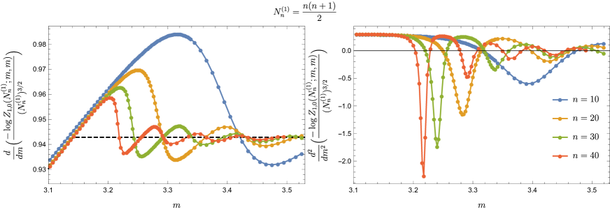
Figure 6: The first- and second derivative of the free energy for $k=1,M=0,N=N_{n}^{(k=1)}$ and $m_{1}=m_{2}=m$ with respect to $m$, calculated by numerical derivatives with $\frac{25}{10000}\leq\Delta m\leq\frac{100}{10000}$. The dashed black line in the left plot is the expected large $n$ asymptotics in $m<\pi$ (5.4) and $m>\pi$ (5.22).

6 Discussion

In this paper we have revisited the large $N$ expansion of the partition function of the mass deformed ABJ theory in the M-theory limit, $N\rightarrow\infty$ with $k$ kept finite. In the previous analyses [104, 103, 106] it was suggested that the partition function exhibits a large $N$ phase transition at $\sqrt{m_{1}m_{2}}=\pi$, above which the large $N$ expansion in the small mass regime given by the Airy function becomes invalid, while large $N$ behavior of the partition function in the supercritical regime was elusive due to the lack of the method of analysis. In this paper we have found a new recursion relation for the partition function with respect to $N$, which enable us to generate exact (or numerical in arbitrarily high precision) values of the partition function at finite but large $N$ which we practically could not reach by the iterative calculation using TBA-like structure of the density matrix [155, 156, 54, 149] (or its numerical approximation) used in the previous analysis. Using these exact values we have revealed various novel properties of the partition function in the supercritical regime. First, although it was observed that the partition function in the supercritical regime oscillates around zero as function of the mass parameters for generic values of $N$, we have found that for each $k$ there is an infinite series of special values $N^{(k)}_{n}$ of the rank $N$ for which the partition function is positive definite even in the supercritical regime. For these special ranks we have further found simple formulas for the large mass asymptotics of the free energy $-\log Z_{k,0}(N^{(k)}_{n})$ for finite $n$ and various values of $k$, which scales as $-\log Z_{k,0}(N^{(k)}_{n})\sim(N^{(k)}_{n})^{3/2}$ in the limit $n\rightarrow\infty$. Interestingly, we observe that the leading behavior (as well as the sub-leading behavior) in the large $n$ limit is valid even when the mass parameters are finite in the supercricial regime. This allows us to make a quantitative proposal for the discontinuity of the large $N$ free energy at $\sqrt{m_{1}m_{2}}=\pi$ as (1.1).

There are various directions of research related to these results which we hope to address in future.

In our analysis the connection between the matrix model for the partition function of the mass deformed ABJ theory and a $\mathfrak{q}$-difference system (3.11),(3.12) has played a crucial role. It is interesting to ask whether similar connection exists for other matrix models. As we mentioned in section 1, when the matrix model is written in the Fermi gas formalism the inverse of whose density matrix defines a five-dimensional ${\cal N}=1$ gauge theory, the connection between the matrix model and a $\mathfrak{q}$-difference system is expected due to the conjecture of the TS/ST correspondence and the Nakajima-Yoshioka blowup equations for the five-dimensional Nekrasov partition function. Indeed it was checked that the grand partition function of a four-node circular quiver Chern-Simons theory, which has the Fermi gas formalism related to the five-dimensional ${\cal N}=1$ $\text{SU}(2)$ Yang-Mills theory with $N_{\text{f}}=4$ fundamental matter fields, satisfies the $\mathfrak{q}$-Painlevé VI equation in $\tau$-form [136, 167, 168]. It would be interesting to investigate similar connection for other circular quiver super Chern-Simons theory whose Fermi gas formalism is related to the five-dimensional linear quiver Yang-Mills theories (see e.g. [169]) and also for the super Chern-Simons theory on affine $D$-type quiver [41] which has the Fermi gas formalism but the corresponding five-dimensional theory is not clear [170, 171].

It would also be interesting to provide physical interpretations to the behavior of the partition function in the supercritical regime from the viewpoint of three-dimensional field theory. Among various properties of the partition function we have found, a simplest one to investigate would be the large mass asymptotics. As listed in table 1 for special values of $N$’s for each $k$, $N^{(k)}_{n}$, and in (5.16),(5.19) for general $N$’s for $k=1,2$, the partition function of the mass deformed ABJM theory in the large mass limit depends on the mass parameters $m_{1},m_{2}$ as $Z_{k,M}(N)\sim e^{-\nu^{(k)}(N)\frac{m_{1}+m_{2}}{2}}$ with $\nu^{(k)}(N)$ some integer smaller than the number of the components of the matter fields $N^{2}$. As mentioned in section 1, the same discrepancy of the exponent is known for the large mass asymptotics of the partition function of three-dimensional supersymmetric gauge theories without Chern-Simons terms. In these setups the discrepancy occurrs when the Coulomb moduli is chosen to non-zero values depending on the mass parameters such that the masses of the matter fields effectively and also new massive degrees of freedom appears as $W$-bosons. This picture is also visible in the integrals in the localization formula for the partition function on $S^{3}$ [172, 173, 174, 175]. Namely, the large mass asymptotics of the partition function can be obtained by assuming that the integration over the Coulomb moduli is dominated by the contributions where the moduli are shifted by the mass parameters in a certain way corresponding to the selected vacuum. Also in the mass deformed ABJM theory we can study the behavior of the integrand in the localization formula (2.3) in the large mass limit when the Coulomb moduli $x_{i},y_{i}$ are shifted by the mass parameters $m_{1},m_{2}$. For simplicity, here let us assume $m_{1}=m_{2}=m$ and consider only the shifts which are identical in $x_{i}$ and $y_{i}$. The ways to shift the Coulomb moduli can be characterized by an integer partition $\lambda=(\lambda_{1},\lambda_{2},\cdots,\lambda_{L})$ of $N$ together with $L$ distinctive real numbers $\{c_{a}\}_{a=1}^{L}$ as follows

$$x_{i}=c_{a}m+\delta x_{i}\quad\Bigl{(}\sum_{b=1}^{a-1}\lambda_{b}+1\leq i\leq\sum_{b=1}^{a}\lambda_{b}\Bigr{)},$$ (6.1)

where $\delta x_{i}$ are of order ${\cal O}(m^{0})$ in the limit of $m\rightarrow\infty$. If we ignore the Chern-Simons factors $e^{\frac{ik}{4\pi}(x_{i}^{2}-y_{i}^{2})}$ and focus only on the one-loop determinant factors

$$Z_{\text{1-loop}}=\frac{\prod_{i<j}^{N}(2\sinh\frac{x_{i}-x_{j}}{2})^{2}\prod_{i<j}^{N}(2\sinh\frac{y_{i}-y_{j}}{2})^{2}}{\prod_{\pm}\prod_{i,j}^{N}2\cosh\frac{x_{i}-y_{j}\pm m}{2}},$$ (6.2)

then we find the following large mass asymptotics for each $\lambda$ and $\{c_{a}\}$:

$$Z_{\text{1-loop}}\sim e^{-m\omega_{\lambda}(\{c_{a}\})},$$ (6.3)

with

$$\omega_{\lambda}(\{c_{a}\})=-2\sum_{a<b}^{L}|c_{a}-c_{b}|\lambda_{a}\lambda_{b}+\frac{1}{2}\sum_{\pm}\sum_{a,b=1}^{L}|c_{a}-c_{b}\pm 1|\lambda_{a}\lambda_{b}.$$ (6.4)

When $c_{a}$’s are separated at least by $1$, i.e. $|c_{a}-c_{b}|\geq 1$, this $\omega_{\lambda}(\{c_{a}\})$ simply reduces to

$$\omega_{\lambda}(\{c_{a}\})=\sum_{a=1}^{L}\lambda_{a}^{2}.$$ (6.5)

Therefore, the exponent listed in table 1 for each $k$ and $N=N^{(k)}_{n}$ is realized, for example, by

1N(1)nn​(n+1)​(2​n+1)6(n,n−1,⋯,2,1)2N(2)nn​(4​n2−1)3(2n−1,2n−3,⋯,3,1)3N(3)n=3​l−1n39+n22+n2+19=3l3+3​l22−l2(3l−1,3l−4,⋯,5,2)N(3)n=3​l−2n39+n22+n2−19=3l3−3​l22−l2(3l−2,3l−5,⋯,4,1)4N(4)n=2​l2​n33−2​n3=4​l​(4​l2−1)3(4l−2,4l−6,⋯,6,2),fragments 1fragmentsN1𝑛𝑛𝑛12𝑛16fragments(n,n1,⋯,2,1)2fragmentsN2𝑛𝑛4superscript𝑛213fragments(2n1,2n3,⋯,3,1)3fragmentsN3𝑛3𝑙1fragmentssuperscript𝑛39superscript𝑛22𝑛2193l33superscript𝑙22𝑙2fragments(3l1,3l4,⋯,5,2)missing-subexpressionfragmentsN3𝑛3𝑙2fragmentssuperscript𝑛39superscript𝑛22𝑛2193l33superscript𝑙22𝑙2fragments(3l2,3l5,⋯,4,1)4fragmentsN4𝑛2𝑙fragments2superscript𝑛332𝑛34𝑙4superscript𝑙213fragments(4l2,4l6,⋯,6,2)\displaystyle\begin{tabular}[]{|c|c|c|c|}\hline\cr&&&\\[-14.0pt] $k$&$N$&$\nu^{(k)}(N)$&a $\lambda$ s.t.~{}$\nu^{(k)}(N)=\omega_{\lambda}(\{c_{a}\})$\\ \hline\cr&&&\\[-14.0pt] $1$&$N^{(1)}_{n}$&$\frac{n(n+1)(2n+1)}{6}$&$(n,n-1,\cdots,2,1)$\\ \hline\cr&&&\\[-14.0pt] $2$&$N^{(2)}_{n}$&$\frac{n(4n^{2}-1)}{3}$&$(2n-1,2n-3,\cdots,3,1)$\\ \hline\cr&&&\\[-14.0pt] $3$&$N^{(3)}_{n=3l-1}$&$\frac{n^{3}}{9}+\frac{n^{2}}{2}+\frac{n}{2}+\frac{1}{9}=3l^{3}+\frac{3l^{2}}{2}-\frac{l}{2}$&$(3l-1,3l-4,\cdots,5,2)$\\ \cline{2-4}\cr&&&\\[-14.0pt] &$N^{(3)}_{n=3l-2}$&$\frac{n^{3}}{9}+\frac{n^{2}}{2}+\frac{n}{2}-\frac{1}{9}=3l^{3}-\frac{3l^{2}}{2}-\frac{l}{2}$&$(3l-2,3l-5,\cdots,4,1)$\\ \hline\cr&&&\\[-14.0pt] $4$&$N^{(4)}_{n=2l}$&$\frac{2n^{3}}{3}-\frac{2n}{3}=\frac{4l(4l^{2}-1)}{3}$&$(4l-2,4l-6,\cdots,6,2)$\\ \hline\cr\end{tabular},

kNν(k)(N)a λ s.t. =ν(k)(N)ωλ({ca}) kNν(k)(N)a λ s.t. =ν(k)(N)ωλ({ca}) (6.18)

while for $k=3,N=N^{(3)}_{n=3l}$ and $k=4,N=N^{(4)}_{n=4l}$ we did not find such simple infinite sequences. Note that in all cases the chioces of $\lambda$ to realize $\omega_{\lambda}=\nu^{(k)}(N)$ are not unique. Note also that $\nu^{(k)}(N)$ are not the smallest exponent realized by the shifts (6.4). For example, for $k=1,N=3$ we have $\omega_{\lambda=(1,1,1)}=3$, which is smaller than $\nu^{(1)}(3)=5$. Nevertheless, it would be interesting to figure out the choices of $\lambda$ for more general $m_{1},m_{2}$ and $k,N,M$, incorpolate the effect of the Chern-Simons terms and provide physical interpretation for these choices which is possibly related to the fuzzy sphere vacua of the mass deformed ABJ theory [99, 176, 177, 178, 179, 180]. It would also be interesting to obtain a shifted configuration in the large $N$ limit as a solution to the saddle point equation for the partition function, as was done for the theories without Chern-Simons terms in [174]. To find physical interpretation to the supercritical regime it would also be useful to study not only the partition function but also the other physical observables such as correlation functions of supersymmetric Wilson loops.

It would also be interesting to understand the holographic interpretation of the phase transition. In [182] the gravity dual of the mass deformed ABJM theory on $S^{3}$ was constructed in the four dimensional ${\cal N}=8$ gauged supergravity (see also [183, 184, 185]), where the solution is smooth at $\sqrt{m_{1}m_{2}}=\pi$. Note that this is not a contradiction to our result. Indeed, starting from the subcritical regime, the expression for the all order $1/N$ perturbative corrections (5.1) is smooth at any values of $m_{1},m_{2}$, and the phase transition is visible only when we take into account the $1/N$ non-perturbative effects. In the massless case these non-perturbative effects correspond in the gravity side to the closed M2-branes wrapped on a three-cycle in $S^{7}/\mathbb{Z}_{k}$, which are not visible in the four-dimensional supergravity. The fact that the real part of one of the exponents $\omega^{\text{WS}}_{\pm,\pm^{\prime}}$ (5.7) of the non-perturbative effect vanihsies at the phase transition point $\sqrt{m_{1}m_{2}}=\pi$ might suggest that the corresponding M2-instanton in the gravity side becomes unstable at this point. It would be interesting to investigate such instability in the eleven-dimensional uplift of the four-dimensional solution which was written down recently [83]. Note, however, that in [83] the authors considered the deformation of the partition function as the $R$-charge deformation, which corresponds to $m_{1},m_{2}\in i\mathbb{R}$. If we formally continue the solutions to $m_{1},m_{2}\in\mathbb{R}$ some components of the metric become complex. Hence it is not clear whether it would be reasonable to analyze the gravity dual of the real mass deformation $m_{1},m_{2}\in\mathbb{R}$ based on the solution in [83] even in the sub-critical regime. We would like to postpone this problem for future research.

Lastly, besides the Fermi gas formalism and the recursion relation, there are different methods proposed to analyze the partition function of the mass deformed ABJM theory such as [187, 188]. It would be interesting to use these methods to understand or analytically derive various properties of the partition function of the mass deformed ABJ theory in the supercritical regime which we have found rather experimentally by using the recursion relation.

Appendix A Exact values of $Z_{k,M}(N;m_{1},m_{2})$

In this appendix we display the exact values of the partition function for relatively small $k$ and $N$ calculated by the method in [149], which are useful for guessing/checking the bilinear relations (3.12),(4.8). Here we display only the results for $M\leq\lfloor\frac{k}{2}\rfloor$, since the partition function for $\lfloor\frac{k}{2}\rfloor<M\leq k$ can be obtained by using the Seiberg-like duality (3.16) which is proved rigorously by using the integration identity (3.14).

For $N=0$ and $N=1,M=0$ we have

$$Z_{k,M}(0)=Z_{k,M}(0,m_{1},m_{2})=i^{\frac{M^{2}}{2}-M}e^{-\frac{\pi iM(M^{2}-1)}{6k}}k^{-\frac{M}{2}}\prod_{r>s}^{M}2\sin\frac{\pi(r-s)}{k},\quad Z_{k,0}(1;m_{1},m_{2})=\frac{1}{4k\cosh\frac{m_{1}}{2}\cosh\frac{m_{2}}{2}}.$$ (A.1)

For $k=1,M=0,N\geq 2$ we have

$$Z_{1,0}(2;m_{1},m_{2})=\frac{\sin\frac{m_{1}m_{2}}{2\pi}}{8\cosh\frac{m_{1}}{2}\cosh\frac{m_{2}}{2}\sinh m_{1}\sinh m_{2}},$$

$$Z_{1,0}(3;m_{1},m_{2})=\frac{1}{32\cosh\frac{m_{1}}{2}\cosh\frac{m_{2}}{2}\cosh\frac{3m_{1}}{2}\cosh\frac{3m_{2}}{2}\sinh m_{1}\sinh m_{2}}\Bigl{(}2\sinh\frac{m_{1}}{2}\sinh\frac{m_{2}}{2}-\sin\frac{3m_{1}m_{2}}{2\pi}\Bigr{)},$$

$$Z_{1,0}(4;m_{1},m_{2})=\frac{1}{128\cosh\frac{m_{1}}{2}\cosh\frac{m_{2}}{2}\sinh m_{1}\sinh m_{2}\cosh\frac{3m_{1}}{2}\cosh\frac{3m_{2}}{2}\sinh 2m_{1}\sinh 2m_{2}}$$

$$\quad\times\Bigl{(}2\cosh m_{1}\cosh m_{2}-\frac{\cosh\frac{3m_{1}}{2}\cosh\frac{3m_{2}}{2}}{\cosh\frac{m_{1}}{2}\cosh\frac{m_{2}}{2}}\cos\frac{m_{1}m_{2}}{\pi}-\cos\frac{3m_{1}m_{2}}{\pi}\Bigr{)},\quad\cdots.$$ (A.2)

For $k=2,M=0,N\geq 2$ we have

$$Z_{2,0}(2;m_{1},m_{2})=\frac{1}{16\sinh^{2}m_{1}\sinh^{2}m_{2}}\Bigl{(}1-\cos\frac{m_{1}m_{2}}{\pi}\Bigr{)},$$

$$Z_{2,0}(3;m_{1},m_{2})=\frac{1}{64\sinh m_{1}\sinh m_{2}\cosh\frac{3m_{1}}{2}\cosh\frac{3m_{2}}{2}\sinh 2m_{1}\sinh 2m_{2}}$$

$$\quad\times\Bigl{(}2\cosh m_{1}\cosh m_{2}-\frac{\cosh\frac{3m_{1}}{2}\cosh\frac{3m_{2}}{2}}{2\cosh\frac{m_{1}}{2}\cosh\frac{m_{2}}{2}}\cos\frac{m_{1}m_{2}}{\pi}-\cos\frac{3m_{1}m_{2}}{\pi}\Bigr{)},$$

$$Z_{2,0}(4;m_{1},m_{2})=\frac{1}{256\sinh m_{1}\sinh m_{2}\sinh^{2}2m_{1}\sinh^{2}2m_{2}\sinh 3m_{1}\sinh 3m_{2}}\Bigl{(}-2\cosh 2m_{1}-2\cosh 2m_{2}$$

$$\quad-8\cosh 2m_{1}\cosh 2m_{2}+8\sinh^{3}\frac{m_{1}}{2}\sinh^{3}\frac{m_{2}}{2}\sinh\frac{3m_{1}}{2}\sinh\frac{3m_{2}}{2}$$

$$\quad+\frac{3\sinh 3m_{1}\sinh 3m_{2}}{\sinh m_{1}\sinh m_{2}}\cos\frac{2m_{1}m_{2}}{\pi}-16\cosh^{2}m_{1}\cosh^{2}m_{2}\cos\frac{3m_{1}m_{2}}{\pi}+\cos\frac{6m_{1}m_{2}}{\pi}\Bigr{)},\quad\cdots.$$ (A.3)

For $k=2,M=1,N\geq 1$ we have

$$Z_{2,1}(1;m_{1},m_{2})=\frac{e^{\frac{\pi i}{4}+\frac{m_{1}+m_{2}}{2}-\frac{im_{1}m_{2}}{2\pi}}\sin\frac{m_{1}m_{2}}{2\pi}}{2\sqrt{2}\sinh m_{1}\sinh m_{2}},$$

$$Z_{2,1}(2;m_{1},m_{2})=\frac{e^{\frac{3\pi i}{4}+m_{1}+m_{2}-\frac{im_{1}m_{2}}{\pi}}}{8\sqrt{2}\sinh m_{1}\sinh m_{2}\sinh 2m_{1}\sinh 2m_{2}}\Bigl{(}-\cosh m_{1}-\cosh m_{2}+\cosh m_{1}\cosh m_{2}+\cos\frac{2m_{1}m_{2}}{\pi}\Bigr{)},$$

$$Z_{2,1}(3;m_{1},m_{2})=\frac{e^{\frac{5\pi i}{4}+\frac{3(m_{1}+m_{2})}{2}-\frac{3im_{1}m_{2}}{2\pi}}}{32\sqrt{2}\sinh m_{1}\sinh m_{2}\sinh 2m_{1}\sinh 2m_{2}\sinh 3m_{1}\sinh 3m_{2}}\Bigl{[}\frac{\sinh 3m_{1}\sinh 3m_{2}}{\sinh m_{1}\sinh m_{2}}\sin\frac{m_{1}m_{2}}{2\pi}$$

$$\quad-2\Bigl{(}\frac{\cosh m_{1}\cosh m_{2}\cosh\frac{3m_{1}}{2}\cosh\frac{3m_{2}}{2}}{\cosh\frac{m_{1}}{2}\cosh\frac{m_{2}}{2}}+\cosh m_{1}+\cosh m_{2}\Bigr{)}\sin\frac{3m_{1}m_{2}}{2\pi}+\sin\frac{9m_{1}m_{2}}{2\pi}\Bigr{]},\quad\cdots.$$ (A.4)

For $k=3,M=0,N\geq 2$ we have

$$Z_{3,0}(2;m_{1},m_{2})=\frac{1}{24\sinh m_{1}\sinh m_{2}\cosh\frac{3m_{1}}{2}\cosh\frac{3m_{2}}{2}}\Bigl{(}2\sinh\frac{m_{1}}{2}\sinh\frac{m_{2}}{2}-\sin\frac{3m_{1}m_{2}}{2\pi}\Bigr{)},$$

$$Z_{3,0}(3;m_{1},m_{2})=\frac{1}{96\cosh^{2}\frac{3m_{1}}{2}\cosh^{2}\frac{3m_{2}}{2}\sinh 3m_{1}\sinh 3m_{2}}\Bigl{(}8\sinh\frac{3m_{1}}{2}\sinh\frac{3m_{2}}{2}$$

$$\quad-\frac{32\sqrt{3}\cosh^{2}\frac{m_{1}}{2}\cosh^{2}\frac{m_{1}}{2}\sinh m_{1}\sinh m_{2}}{3}\cos\frac{3m_{1}m_{2}}{2\pi}$$

$$\quad-2(\cosh 2m_{1}-2\cosh m_{1})(\cosh 2m_{2}-2\cosh m_{2})\sin\frac{3m_{1}m_{2}}{2\pi}+\sin\frac{9m_{1}m_{2}}{2\pi}\Bigr{)},\quad\cdots.$$ (A.5)

For $k=3,M=1,N\geq 1$ we have

$$Z_{3,1}(1;m_{1},m_{2})=\frac{e^{\frac{3\pi i}{4}+\frac{m_{1}+m_{2}}{2}}}{4\sqrt{3}\cosh\frac{3m_{1}}{2}\cosh\frac{3m_{2}}{2}}\Bigl{[}ie^{-\frac{3im_{1}m_{2}}{2\pi}}-2\sinh\frac{m_{1}}{2}\sinh\frac{m_{2}}{2}-\frac{2i\cosh\frac{m_{1}}{2}\cosh\frac{m_{2}}{2}}{\sqrt{3}}\Bigr{]},$$

$$Z_{3,1}(2;m_{1},m_{2})=\frac{e^{\frac{3\pi i}{4}+m_{1}+m_{2}}}{16\sqrt{3}\cosh\frac{3m_{1}}{2}\cosh\frac{3m_{2}}{2}\sinh 3m_{1}\sinh 3m_{2}}\biggl{[}-ie^{-\frac{9im_{1}m_{2}}{2\pi}}$$

$$\quad+\biggl{(}\frac{4\sinh m_{1}\sinh m_{2}(1+\cosh m_{1}+\cosh m_{2})}{\sqrt{3}}+i\Bigl{(}\frac{4\sinh^{2}\frac{m_{1}}{2}\sinh^{2}\frac{m_{2}}{2}(4\cosh m_{1}+1)(4\cosh m_{2}+1)}{3}$$

$$\quad\quad+\cosh m_{1}+\cosh m_{2}+\cosh m_{1}\cosh m_{2}\Bigr{)}\biggr{)}e^{-\frac{3im_{1}m_{2}}{2\pi}}$$

$$\quad-4\sinh\frac{3m_{1}}{2}\sinh\frac{3m_{2}}{2}+\Bigl{(}\frac{2i\sinh m_{1}\sinh m_{2}}{\sqrt{3}}-2i\cosh m_{1}\cosh m_{2}\Bigr{)}e^{\frac{3im_{1}m_{2}}{2\pi}}\biggr{]},\quad\cdots.$$ (A.6)

Appendix B Guess of bilinear relation for $m_{1}\neq m_{2}$ (3.12) from exact values

In section 3 we have displayed the bilinear relation (3.12) for $1\leq M\leq k-1$ and its extension (4.8) to $M=0$. As explained in section 3, (4.8) can be straightforwardly guessed from (3.12) by applying the duality relations (4.7) to $\Xi_{k,-1}(\kappa)$, while (3.12) for $m_{1}=m_{2}$, namely (3.11), was guessed from the topological string/spectral theory correspondence and the blowup relation in the corresponding topological string (or five-dimensional super Yang-Mills) side. On the other hand, so far there is no such justification for the bilinear relation with $m_{1}\neq m_{2}$ (3.12). Instead we have found (3.12) by assuming that the bilinear relation of the following form holds

$$\sum_{i=1}^{L_{1}}a_{i}\Xi_{k,M+1}(b_{i}\kappa;m_{1},m_{2})\Xi_{k,M-1}(c_{i}\kappa;m_{1},m_{2})+\sum_{i=1}^{L_{2}}d_{i}\Xi_{1,M}(e_{i}\kappa;m_{1},m_{2})\Xi_{1,M}(f_{i}\kappa;m_{1},m_{2})=0,$$ (B.1)

for some $L_{1},L_{2}\geq 0$ and some coefficients $a_{i},b_{i},c_{i},d_{i},e_{i},f_{i}$, and then fixing these parameters by using the exact values of the partition function (A.1)-(A.6). In this appendix we demonstrate how this guesswork goes.

For simplicity let us consider the case $k=1$, where the bilinear relation should be written only in terms of $Z_{1,0}(N;m_{1},m_{2})$ after using the duality relations as

$$\kappa\sum_{i=1}^{L_{1}}a^{\prime}_{i}\Xi_{1,0}(b^{\prime}_{i}\kappa;m_{1},m_{2})\Xi_{1,0}(c^{\prime}_{i}\kappa;m_{1},m_{2})+\sum_{i=1}^{L_{2}}d_{i}\Xi_{1,0}(e_{i}\kappa;m_{1},m_{2})\Xi_{1,0}(f_{i}\kappa;m_{1},m_{2})=0.$$ (B.2)

Here $a_{i}^{\prime},b_{i}^{\prime},c_{i}^{\prime}$ are related to $a_{i},b_{i},c_{i}$ in (B.1) as

$$a_{i}^{\prime}=e^{-\frac{m_{1}+m_{2}}{2}}a_{i}c_{i},\quad b_{i}^{\prime}=ie^{\frac{m_{1}+m_{2}}{2}-\frac{im_{1}m_{2}}{2\pi}}b_{i},\quad c_{i}^{\prime}=-ie^{-\frac{m_{1}+m_{2}}{2}+\frac{im_{1}m_{2}}{2\pi}}c_{i}.$$ (B.3)

We also require that for $m_{1}=m_{2}=m$ the bilinear relation reduces to the following

$$\kappa\Xi_{1,0}(-ie^{-\frac{im^{2}}{2\pi}}\kappa;m,m)\Xi_{1,0}(ie^{\frac{im^{2}}{2\pi}}\kappa;m,m)+\Xi_{1,0}(-e^{m}\kappa;m,m)\Xi_{1,0}(-e^{-m}\kappa;m,m)$$

$$\quad-\Xi_{1,0}(\kappa;m,m)\Xi_{1,0}(\kappa;m,m)=0,$$ (B.4)

as obtained from (3.11) and (4.7). By expanding the left-hand side of (B.2) in $\kappa$, we obtain the following constraints from the orders $\kappa^{0},\kappa^{1},\kappa^{2}$

$$\sum_{i=1}^{L_{2}}d_{i}=0,$$ (B.5)

$$\sum_{i=1}^{L_{1}}a^{\prime}_{i}+\sum_{i=1}^{L_{2}}d_{i}(e_{i}+f_{i})Z_{1,0}(1)=0,$$ (B.6)

$$\sum_{i=1}^{L_{1}}a^{\prime}_{i}(b^{\prime}_{i}+c^{\prime}_{i})Z_{1,0}(1)+\sum_{i=1}^{L_{2}}[d_{i}(e_{i}^{2}+f_{i}^{2})Z_{1,0}(2)+e_{i}f_{i}Z_{1,0}(1)^{2}]=0,$$ (B.7)

where we have used $Z_{1,0}(0)=1$. Let us first look at the second equation. By substituting the exact value $Z_{1,0}(1)=\frac{1}{4\cosh\frac{m_{1}}{2}\cosh\frac{m_{2}}{2}}$ (A.2) we obtain

$$-\frac{\sum_{i=1}^{L_{2}}d_{i}(e_{i}+f_{i})}{\sum_{i=1}^{L_{1}}a_{i}^{\prime}}=e^{\frac{m_{1}+m_{2}}{2}}+e^{\frac{m_{1}-m_{2}}{2}}+e^{\frac{-m_{1}+m_{2}}{2}}+e^{\frac{-m_{1}-m_{2}}{2}}.$$ (B.8)

Taking also into account the equation for $M=0$ (B.4), it is not difficult to guess $L_{2},e_{i},f_{i}$ as

$$L_{2}=2,\quad e_{1}=-e^{\frac{m_{1}+m_{2}}{2}},\quad f_{1}=-e^{-\frac{m_{1}+m_{2}}{2}},\quad e_{2}=e^{\frac{m_{1}-m_{2}}{2}},\quad f_{2}=e^{-\frac{m_{1}-m_{2}}{2}},$$ (B.9)

with which we are left with the following condition on $d_{1},d_{2}$

$$d_{1}=-d_{2}=\sum_{i=1}^{L_{1}}a_{i}^{\prime}.$$ (B.10)

Note that the constraint from the order $\kappa^{0}$ (B.5) is also granted under this condition. Next look at the constraint from the order $\kappa^{2}$ (B.7)

$$Z_{1,0}(2)=-\frac{\sum_{i=1}^{L_{1}}a_{i}^{\prime}(b_{i}^{\prime}+c_{i}^{\prime})Z_{1,0}(1)+\sum_{i=1}^{L_{2}}d_{i}e_{i}f_{i}Z_{1,0}(1)^{2}}{\sum_{i=1}^{L_{2}}d_{i}(e_{i}^{2}+f_{i}^{2})}.$$ (B.11)

After the substition $L_{2},d_{i},e_{i},f_{i}$ fixed above and the exact values of $Z_{1,0}(1)$ and $Z_{1,0}(2)$ (A.2), this reduces to

$$\frac{\sum_{i=1}^{L_{1}}a_{i}^{\prime}(b_{i}^{\prime}+c_{i}^{\prime})}{\sum_{i=1}^{L_{1}}a^{\prime}_{i}}=ie^{\frac{im_{1}m_{2}}{2\pi}}-ie^{-\frac{im_{1}m_{2}}{2\pi}}.$$ (B.12)

from which it is not difficult to guess $L_{1},a_{i}^{\prime},b_{i}^{\prime},c_{i}^{\prime}$ as

$$L_{1}=1,\quad a_{1}^{\prime}=1,\quad b_{1}^{\prime}=-ie^{-\frac{im_{1}m_{2}}{2\pi}},\quad c_{1}^{\prime}=ie^{\frac{im_{1}m_{2}}{2\pi}},$$ (B.13)

which also fixes $d_{1},d_{2}$ as $d_{1}=1,d_{2}=-1$. Once we have guessed the coefficients completely, we can further check that (B.2) is satisfied also for $N\geq 3$ by using the exact values of the partition function.

Plugging these results back to (B.1), now we have the following guess for the bilinear relation at $k=1,M=0$

$$-\Xi_{1,1}(-e^{-\frac{m_{1}+m_{2}}{2}};m_{1},m_{2})\Xi_{1,-1}(-e^{\frac{m_{1}+m_{2}}{2}};m_{1},m_{2})+\Xi_{1,0}(-e^{\frac{m_{1}+m_{2}}{2}};m_{1},m_{2})\Xi_{1,0}(-e^{-\frac{m_{1}+m_{2}}{2}};m_{1},m_{2})$$

$$\quad-\Xi_{1,0}(e^{\frac{m_{1}-m_{2}}{2}};m_{1},m_{2})\Xi_{1,0}(e^{-\frac{m_{1}-m_{2}}{2}};m_{1},m_{2})=0.$$ (B.14)

By choosing the $k,M$-dependent coefficients same as those in the bilinear relation for $m_{1}=m_{2}$ (3.11), we end up with the bilinear relation (3.12) for $m_{1}\neq m_{2}$.

Appendix C Instanton coefficients of $\omega^{\text{WS}}_{\pm,\pm^{\prime}}$

In this appendix we compare our guess for the instanton coefficient for $\omega=\omega^{\text{WS}}_{\pm,\pm^{\prime}}$ (5.12) with the non-perturbative effect lead off from the the numerical values of $Z_{k,M}(N)$. Since the partition function is symmetric under $\mathbb{Z}_{2}\times\mathbb{Z}_{2}$ transformation $m_{1}\rightarrow-m_{1}$ and $m_{2}\rightarrow-m_{2}$, it is sufficient to look at one of the four species, say $\omega^{\text{WS}}_{--}$ which is the most dominant one when $0<-im_{1}<\pi$ and $0<-im_{2}<\pi$ among the four. Note that in order to make this instanton the most dominant one among all species (5.6), we have to choose $m_{1},m_{2}$ such that $\omega^{\text{WS}}_{--}<1$ (we do not have to examine $\omega^{\text{WS}}_{--}<\omega^{\text{MB}}_{i,\pm}$ since $\omega^{\text{MB}}_{i,\pm}$ is always larger than $1$), namely

$$\frac{4}{k(1-\frac{im_{1}}{\pi})(1-\frac{im_{2}}{\pi})}<1.$$ (C.1)

Let us choose a point $(m_{1},m_{2})$ which satisfy the condition (C.1). To extract the instanton coefficient $\gamma(n_{\omega^{\text{WS}}_{--}}=1,\text{other }n_{\omega}=0)$, let us truncate the modified grand potential $J(\mu)$ (5.10) as

$$J(\mu)=\frac{C}{3}\mu^{3}+B\mu+A+\gamma(n_{\omega^{\text{WS}}_{--}}=1,\text{other }n_{\omega}=0)e^{-\omega^{\text{WS}}_{--}\mu}+\cdots.$$ (C.2)

Substituting this into the inversion formula (5.9) we obtain

$$Z_{k,M}(N) =\int\frac{d\mu}{2\pi}e^{\frac{C}{3}\mu^{3}+B\mu+A-\mu N}(1+\gamma(n_{\omega^{\text{WS}}_{--}}=1,\text{other }n_{\omega}=0)e^{-\omega^{\text{WS}}_{--}\mu}+\cdots)$$

$$=Z_{k,M}^{\text{pert}}(N)+Z_{k,M}^{\text{pert}}(N+\omega^{\text{WS}}_{--})\gamma(n_{\omega^{\text{WS}}_{--}}=1,\text{other }n_{\omega}=0)+\cdots.$$ (C.3)

This implies that we can estimate $\gamma(n_{\omega^{\text{WS}}_{--}}=1,\text{other }n_{\omega}=0)$ by comparing the exact (or numerical with high precision) values of $Z_{k,M}(N)$ with $Z_{k,M}^{\text{pert}}(N)$ as

$$\gamma(n_{\omega^{\text{WS}}_{--}}=1,\text{other }n_{\omega}=0)\approx\frac{Z_{k,M}(N)-Z_{k,M}^{\text{pert}}(N)}{Z_{k,M}^{\text{pert}}(N+\omega^{\text{WS}}_{--})}.$$ (C.4)

Note however that in some parameter regime it is difficult to evaluate $Z_{k,M}^{\text{pert}}(N)$ at high precision due to the constant $A$ (5.2) which is given only through the integral representation (5.3) for generic $m_{1},m_{2}$. For this reason it is more useful to extract the instanton coefficient from the ratio of the partition functions at two different $N$’s as

$$\gamma(n_{\omega^{\text{WS}}_{--}}=1,\text{other }n_{\omega}=0)\approx\frac{\frac{Z_{k,M}(N)}{Z_{k,M}(N_{0})}-\frac{Z_{k,M}^{\text{pert}}(N)}{Z_{k,M}^{\text{pert}}(N_{0})}}{\frac{Z_{k,M}^{\text{pert}}(N+\omega^{\text{WS}}_{--})}{Z_{k,M}^{\text{pert}}(N_{0})}-\frac{Z_{k,M}(N)}{Z_{k,M}(N_{0})}\frac{Z_{k,M}^{\text{pert}}(N_{0}+\omega^{\text{WS}}_{--})}{Z_{k,M}^{\text{pert}}(N_{0})}}.$$ (C.5)

By comparing the right-hand side calculated for sufficiently large $N,N_{0}$ with (5.12) we indeed find a good agreement. See figure 7.

$k$	$M$	$m_{1}$	$m_{2}$	(C.5)	(5.12)
$2$	$0$	$\frac{38703i}{25000}$	$\frac{91199i}{50000}$	$0.31757724067372809500$	$0.31757724067286396948$
	$1$	$\frac{38703i}{25000}$	$\frac{91199i}{50000}$	$-0.31757724067201452421$	$-0.31757724067286396948$
$3$	$0$	$\frac{30509i}{50000}$	$\frac{10977i}{12500}$	$0.25479966165669975897$	$0.25479965063727587352$
	$1$	$\frac{30509i}{50000}$	$\frac{10977i}{12500}$	$-0.12739983071109485153$	$-0.12739982531863793676$

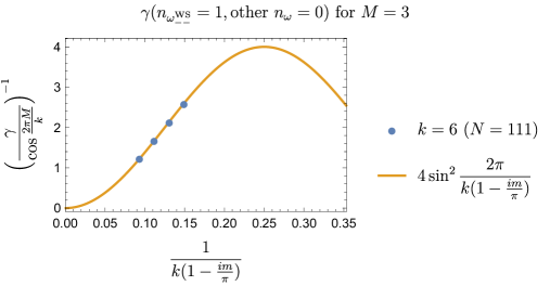
Figure 7: Comparison between $\gamma(n_{\omega^{\text{WS}}_{--}}=1,\text{other }n_{\omega}=0)$ obtained by a numerical extraction (C.5) and the analytic guess (5.12) for $m_{1}\neq m_{2}$ (top table) and $m_{1}=m_{2}=m$ (bottom plots). In the top table we have chosen $N=188$ for $k=2$ and $N=138$ for $k=3$, as also displayed in the plots. We have chosen $N_{0}$ in (C.5) as $N_{0}=N+1$ for all cases. As $Z_{k,M}(N),Z_{k,M}(N_{0})$ we have used the numerical values obtained by the recursion relations (4.12),(4.18),(4.19) with initial conditions set with the precision of $2000$ digits.

References

- [1] J. M. Maldacena, “The Large N limit of superconformal field theories and supergravity,” Adv.Theor.Math.Phys. 2 (1998) 231–252, arXiv:hep-th/9711200 [hep-th].
- [2] K. Hosomichi, K.-M. Lee, S. Lee, S. Lee, and J. Park, “N=4 Superconformal Chern-Simons Theories with Hyper and Twisted Hyper Multiplets,” JHEP 07 (2008) 091, arXiv:0805.3662 [hep-th].
- [3] O. Aharony, O. Bergman, D. L. Jafferis, and J. Maldacena, “N=6 superconformal Chern-Simons-matter theories, M2-branes and their gravity duals,” JHEP 0810 (2008) 091, arXiv:0806.1218 [hep-th].
- [4] O. Aharony, O. Bergman, and D. L. Jafferis, “Fractional M2-branes,” JHEP 11 (2008) 043, arXiv:0807.4924 [hep-th].
- [5] S. Mukhi and C. Papageorgakis, “M2 to D2,” JHEP 05 (2008) 085, arXiv:0803.3218 [hep-th].
- [6] Y. Pang and T. Wang, “From N M2’s to N D2’s,” Phys. Rev. D 78 (2008) 125007, arXiv:0807.1444 [hep-th].
- [7] I. Jeon, N. Lambert, and P. Richmond, “Periodic Arrays of M2-Branes,” JHEP 11 (2012) 100, arXiv:1206.6699 [hep-th].
- [8] A. Gustavsson and S.-J. Rey, “Enhanced N=8 Supersymmetry of ABJM Theory on R**8 and R**8/Z(2),” arXiv:0906.3568 [hep-th].
- [9] O.-K. Kwon, P. Oh, and J. Sohn, “Notes on Supersymmetry Enhancement of ABJM Theory,” JHEP 08 (2009) 093, arXiv:0906.4333 [hep-th].
- [10] D. Bashkirov and A. Kapustin, “Supersymmetry enhancement by monopole operators,” JHEP 05 (2011) 015, arXiv:1007.4861 [hep-th].
- [11] D. Bashkirov and A. Kapustin, “Dualities between N = 8 superconformal field theories in three dimensions,” JHEP 05 (2011) 074, arXiv:1103.3548 [hep-th].
- [12] K. Jensen and A. Karch, “ABJM Mirrors and a Duality of Dualities,” JHEP 09 (2009) 004, arXiv:0906.3013 [hep-th].
- [13] N. Lambert and C. Papageorgakis, “Relating U(N)xU(N) to SU(N)xSU(N) Chern-Simons Membrane theories,” JHEP 1004 (2010) 104, arXiv:1001.4779 [hep-th].
- [14] A. Basu and J. A. Harvey, “The M2-M5 brane system and a generalized Nahm’s equation,” Nucl. Phys. B 713 (2005) 136–150, arXiv:hep-th/0412310.
- [15] A. Gustavsson, “Selfdual strings and loop space Nahm equations,” JHEP 0804 (2008) 083, arXiv:0802.3456 [hep-th].
- [16] H. Nastase, C. Papageorgakis, and S. Ramgoolam, “The Fuzzy S**2 structure of M2-M5 systems in ABJM membrane theories,” JHEP 05 (2009) 123, arXiv:0903.3966 [hep-th].
- [17] S. Terashima and F. Yagi, “M5-brane Solution in ABJM Theory and Three-algebra,” JHEP 12 (2009) 059, arXiv:0909.3101 [hep-th].
- [18] N. Lambert and C. Papageorgakis, “Nonabelian (2,0) Tensor Multiplets and 3-algebras,” JHEP 08 (2010) 083, arXiv:1007.2982 [hep-th].
- [19] T. Nosaka and S. Terashima, “M5-branes in ABJM theory and Nahm equation,” Phys. Rev. D 86 (2012) 125027, arXiv:1208.1108 [hep-th].
- [20] K. Sakai and S. Terashima, “Integrability of BPS equations in ABJM theory,” JHEP 11 (2013) 002, arXiv:1308.3583 [hep-th].
- [21] V. Pestun, “Localization of gauge theory on a four-sphere and supersymmetric Wilson loops,” Commun. Math. Phys. 313 (2012) 71–129, arXiv:0712.2824 [hep-th].
- [22] A. Kapustin, B. Willett, and I. Yaakov, “Nonperturbative Tests of Three-Dimensional Dualities,” JHEP 10 (2010) 013, arXiv:1003.5694 [hep-th].
- [23] D. L. Jafferis, “The Exact Superconformal R-Symmetry Extremizes Z,” JHEP 05 (2012) 159, arXiv:1012.3210 [hep-th].
- [24] N. Hama, K. Hosomichi, and S. Lee, “Notes on SUSY Gauge Theories on Three-Sphere,” JHEP 03 (2011) 127, arXiv:1012.3512 [hep-th].
- [25] N. Hama, K. Hosomichi, and S. Lee, “SUSY Gauge Theories on Squashed Three-Spheres,” JHEP 05 (2011) 014, arXiv:1102.4716 [hep-th].
- [26] I. R. Klebanov and A. A. Tseytlin, “Near extremal black hole entropy and fluctuating three-branes,” Nucl. Phys. B 479 (1996) 319–335, arXiv:hep-th/9607107.
- [27] N. Drukker, M. Marino, and P. Putrov, “From weak to strong coupling in ABJM theory,” Commun. Math. Phys. 306 (2011) 511–563, arXiv:1007.3837 [hep-th].
- [28] C. P. Herzog, I. R. Klebanov, S. S. Pufu, and T. Tesileanu, “Multi-Matrix Models and Tri-Sasaki Einstein Spaces,” Phys. Rev. D 83 (2011) 046001, arXiv:1011.5487 [hep-th].
- [29] R. C. Santamaria, M. Marino, and P. Putrov, “Unquenched flavor and tropical geometry in strongly coupled Chern-Simons-matter theories,” JHEP 10 (2011) 139, arXiv:1011.6281 [hep-th].
- [30] N. Drukker, M. Marino, and P. Putrov, “Nonperturbative aspects of ABJM theory,” JHEP 11 (2011) 141, arXiv:1103.4844 [hep-th].
- [31] H. Fuji, S. Hirano, and S. Moriyama, “Summing Up All Genus Free Energy of ABJM Matrix Model,” JHEP 08 (2011) 001, arXiv:1106.4631 [hep-th].
- [32] M. Hanada, M. Honda, Y. Honma, J. Nishimura, S. Shiba, and Y. Yoshida, “Numerical studies of the ABJM theory for arbitrary N at arbitrary coupling constant,” JHEP 05 (2012) 121, arXiv:1202.5300 [hep-th].
- [33] M. Honda, M. Hanada, Y. Honma, J. Nishimura, S. Shiba, and Y. Yoshida, “Monte Carlo studies of 3d N=6 SCFT via localization method,” PoS LATTICE2012 (2012) 233, arXiv:1211.6844 [hep-lat].
- [34] A. Amariti, C. Klare, and M. Siani, “The Large N Limit of Toric Chern-Simons Matter Theories and Their Duals,” JHEP 10 (2012) 019, arXiv:1111.1723 [hep-th].
- [35] D. Gang, C. Hwang, S. Kim, and J. Park, “Tests of AdS4/CFT3 correspondence for chiral-like theory,” JHEP 02 (2012) 079, arXiv:1111.4529 [hep-th].
- [36] D. Martelli and J. Sparks, “The large N limit of quiver matrix models and Sasaki-Einstein manifolds,” Phys. Rev. D 84 (2011) 046008, arXiv:1102.5289 [hep-th].
- [37] S. Cheon, H. Kim, and N. Kim, “Calculating the partition function of N=2 Gauge theories on and AdS/CFT correspondence,” JHEP 05 (2011) 134, arXiv:1102.5565 [hep-th].
- [38] A. Amariti and S. Franco, “Free Energy vs Sasaki-Einstein Volume for Infinite Families of M2-Brane Theories,” JHEP 09 (2012) 034, arXiv:1204.6040 [hep-th].
- [39] J. T. Liu and X. Zhang, “The large- partition function for non-parity-invariant Chern-Simons-matter theories,” JHEP 12 (2020) 007, arXiv:2008.09642 [hep-th].
- [40] D. R. Gulotta, J. P. Ang, and C. P. Herzog, “Matrix Models for Supersymmetric Chern-Simons Theories with an ADE Classification,” JHEP 01 (2012) 132, arXiv:1111.1744 [hep-th].
- [41] P. M. Crichigno, C. P. Herzog, and D. Jain, “Free Energy of Quiver Chern-Simons Theories,” JHEP 03 (2013) 039, arXiv:1211.1388 [hep-th].
- [42] A. Amariti, M. Fazzi, N. Mekareeya, and A. Nedelin, “New 3d SCFT’s with scaling,” JHEP 12 (2019) 111, arXiv:1903.02586 [hep-th].
- [43] D. R. Gulotta, C. P. Herzog, and T. Nishioka, “The ABCDEF’s of Matrix Models for Supersymmetric Chern-Simons Theories,” JHEP 04 (2012) 138, arXiv:1201.6360 [hep-th].
- [44] D. L. Jafferis, I. R. Klebanov, S. S. Pufu, and B. R. Safdi, “Towards the F-Theorem: N=2 Field Theories on the Three-Sphere,” JHEP 06 (2011) 102, arXiv:1103.1181 [hep-th].
- [45] D. Jain, “Deconstructing Deformed D-quivers,” arXiv:1512.08955 [hep-th].
- [46] Y. Imamura and D. Yokoyama, “N=2 supersymmetric theories on squashed three-sphere,” Phys. Rev. D 85 (2012) 025015, arXiv:1109.4734 [hep-th].
- [47] L. F. Alday, M. Fluder, and J. Sparks, “The Large N limit of M2-branes on Lens spaces,” JHEP 10 (2012) 057, arXiv:1204.1280 [hep-th].
- [48] M. Mariño and P. Putrov, “Interacting fermions and N=2 Chern-Simons-matter theories,” JHEP 11 (2013) 199, arXiv:1206.6346 [hep-th].
- [49] Y. Hatsuda, “ABJM on ellipsoid and topological strings,” JHEP 07 (2016) 026, arXiv:1601.02728 [hep-th].
- [50] M. Marino and P. Putrov, “ABJM theory as a Fermi gas,” J. Stat. Mech. 1203 (2012) P03001, arXiv:1110.4066 [hep-th].
- [51] H. Awata, S. Hirano, and M. Shigemori, “The Partition Function of ABJ Theory,” PTEP 2013 (2013) 053B04, arXiv:1212.2966 [hep-th].
- [52] M. Honda, “Direct derivation of ”mirror” ABJ partition function,” JHEP 12 (2013) 046, arXiv:1310.3126 [hep-th].
- [53] S. Matsumoto and S. Moriyama, “ABJ Fractional Brane from ABJM Wilson Loop,” JHEP 03 (2014) 079, arXiv:1310.8051 [hep-th].
- [54] P. Putrov and M. Yamazaki, “Exact ABJM Partition Function from TBA,” Mod. Phys. Lett. A 27 (2012) 1250200, arXiv:1207.5066 [hep-th].
- [55] Y. Hatsuda, S. Moriyama, and K. Okuyama, “Instanton Effects in ABJM Theory from Fermi Gas Approach,” JHEP 01 (2013) 158, arXiv:1211.1251 [hep-th].
- [56] F. Calvo and M. Marino, “Membrane instantons from a semiclassical TBA,” JHEP 05 (2013) 006, arXiv:1212.5118 [hep-th].
- [57] Y. Hatsuda, S. Moriyama, and K. Okuyama, “Instanton Bound States in ABJM Theory,” JHEP 05 (2013) 054, arXiv:1301.5184 [hep-th].
- [58] Y. Hatsuda, S. Moriyama, and K. Okuyama, “Exact Results on the ABJM Fermi Gas,” JHEP 10 (2012) 020, arXiv:1207.4283 [hep-th].
- [59] M. Mezei and S. S. Pufu, “Three-sphere free energy for classical gauge groups,” JHEP 02 (2014) 037, arXiv:1312.0920 [hep-th].
- [60] A. Grassi and M. Marino, “M-theoretic matrix models,” JHEP 02 (2015) 115, arXiv:1403.4276 [hep-th].
- [61] M. Honda and S. Moriyama, “Instanton Effects in Orbifold ABJM Theory,” JHEP 08 (2014) 091, arXiv:1404.0676 [hep-th].
- [62] Y. Hatsuda and K. Okuyama, “Probing non-perturbative effects in M-theory,” JHEP 10 (2014) 158, arXiv:1407.3786 [hep-th].
- [63] S. Moriyama and T. Nosaka, “Partition Functions of Superconformal Chern-Simons Theories from Fermi Gas Approach,” JHEP 11 (2014) 164, arXiv:1407.4268 [hep-th].
- [64] S. Moriyama and T. Nosaka, “ABJM membrane instanton from a pole cancellation mechanism,” Phys. Rev. D 92 no. 2, (2015) 026003, arXiv:1410.4918 [hep-th].
- [65] Y. Hatsuda, M. Honda, and K. Okuyama, “Large N non-perturbative effects in superconformal Chern-Simons theories,” JHEP 09 (2015) 046, arXiv:1505.07120 [hep-th].
- [66] S. Moriyama and T. Suyama, “Instanton Effects in Orientifold ABJM Theory,” JHEP 03 (2016) 034, arXiv:1511.01660 [hep-th].
- [67] M. Honda, “Exact relations between M2-brane theories with and without Orientifolds,” JHEP 06 (2016) 123, arXiv:1512.04335 [hep-th].
- [68] K. Okuyama, “Orientifolding of the ABJ Fermi gas,” JHEP 03 (2016) 008, arXiv:1601.03215 [hep-th].
- [69] S. Moriyama and T. Suyama, “Orthosymplectic Chern-Simons Matrix Model and Chirality Projection,” JHEP 04 (2016) 132, arXiv:1601.03846 [hep-th].
- [70] S. Moriyama and T. Nosaka, “Orientifold ABJM Matrix Model: Chiral Projections and Worldsheet Instantons,” JHEP 06 (2016) 068, arXiv:1603.00615 [hep-th].
- [71] S. Bhattacharyya, A. Grassi, M. Marino, and A. Sen, “A One-Loop Test of Quantum Supergravity,” Class. Quant. Grav. 31 (2014) 015012, arXiv:1210.6057 [hep-th].
- [72] J. T. Liu and W. Zhao, “One-loop supergravity on and comparison with ABJM theory,” JHEP 11 (2016) 099, arXiv:1609.02558 [hep-th].
- [73] N. Bobev, M. David, J. Hong, V. Reys, and X. Zhang, “A compendium of logarithmic corrections in AdS/CFT,” arXiv:2312.08909 [hep-th].
- [74] M. Beccaria and A. A. Tseytlin, “Comments on ABJM free energy on S3 at large N and perturbative expansions in M-theory and string theory,” Nucl. Phys. B 994 (2023) 116286, arXiv:2306.02862 [hep-th].
- [75] N. Bobev, A. M. Charles, K. Hristov, and V. Reys, “The Unreasonable Effectiveness of Higher-Derivative Supergravity in AdS4 Holography,” Phys. Rev. Lett. 125 no. 13, (2020) 131601, arXiv:2006.09390 [hep-th].
- [76] N. Bobev, A. M. Charles, K. Hristov, and V. Reys, “Higher-derivative supergravity, AdS4 holography, and black holes,” JHEP 08 (2021) 173, arXiv:2106.04581 [hep-th].
- [77] K. Hristov and V. Reys, “Factorization of log-corrections in AdS4/CFT3 from supergravity localization,” JHEP 12 (2021) 031, arXiv:2107.12398 [hep-th].
- [78] K. Hristov, “4d = 2 supergravity observables from Nekrasov-like partition functions,” JHEP 02 (2022) 079, arXiv:2111.06903 [hep-th].
- [79] N. Bobev, J. Hong, and V. Reys, “Large N Partition Functions, Holography, and Black Holes,” Phys. Rev. Lett. 129 no. 4, (2022) 041602, arXiv:2203.14981 [hep-th].
- [80] K. Hristov, “ABJM at finite N via 4d supergravity,” JHEP 10 (2022) 190, arXiv:2204.02992 [hep-th].
- [81] N. Bobev, J. Hong, and V. Reys, “Large N partition functions of the ABJM theory,” JHEP 02 (2023) 020, arXiv:2210.09318 [hep-th].
- [82] N. Bobev, J. Hong, and V. Reys, “Large N partition functions of 3d holographic SCFTs,” JHEP 08 (2023) 119, arXiv:2304.01734 [hep-th].
- [83] F. F. Gautason, V. G. M. Puletti, and J. van Muiden, “Quantized strings and instantons in holography,” JHEP 08 (2023) 218, arXiv:2304.12340 [hep-th].
- [84] M. Beccaria, S. Giombi, and A. A. Tseytlin, “Instanton contributions to the ABJM free energy from quantum M2 branes,” arXiv:2307.14112 [hep-th].
- [85] A. Dabholkar, N. Drukker, and J. Gomes, “Localization in supergravity and quantum holography,” JHEP 10 (2014) 090, arXiv:1406.0505 [hep-th].
- [86] P. Caputa and S. Hirano, “Airy Function and 4d Quantum Gravity,” JHEP 06 (2018) 106, arXiv:1804.00942 [hep-th].
- [87] N. B. Agmon, S. M. Chester, and S. S. Pufu, “A new duality between = 8 superconformal field theories in three dimensions,” JHEP 06 (2018) 005, arXiv:1708.07861 [hep-th].
- [88] N. B. Agmon, S. M. Chester, and S. S. Pufu, “Solving M-theory with the Conformal Bootstrap,” JHEP 06 (2018) 159, arXiv:1711.07343 [hep-th].
- [89] S. M. Chester, S. S. Pufu, and X. Yin, “The M-Theory S-Matrix From ABJM: Beyond 11D Supergravity,” JHEP 08 (2018) 115, arXiv:1804.00949 [hep-th].
- [90] D. J. Binder, S. M. Chester, and S. S. Pufu, “Absence of in M-Theory From ABJM,” JHEP 04 (2020) 052, arXiv:1808.10554 [hep-th].
- [91] D. J. Binder, S. M. Chester, and S. S. Pufu, “AdS4/CFT3 from weak to strong string coupling,” JHEP 01 (2020) 034, arXiv:1906.07195 [hep-th].
- [92] N. B. Agmon, S. M. Chester, and S. S. Pufu, “The M-theory Archipelago,” JHEP 02 (2020) 010, arXiv:1907.13222 [hep-th].
- [93] S. M. Chester, R. R. Kalloor, and A. Sharon, “3d = 4 OPE coefficients from Fermi gas,” JHEP 07 (2020) 041, arXiv:2004.13603 [hep-th].
- [94] D. J. Binder, S. M. Chester, M. Jerdee, and S. S. Pufu, “The 3d = 6 bootstrap: from higher spins to strings to membranes,” JHEP 05 (2021) 083, arXiv:2011.05728 [hep-th].
- [95] L. F. Alday, S. M. Chester, and H. Raj, “ABJM at strong coupling from M-theory, localization, and Lorentzian inversion,” JHEP 02 (2022) 005, arXiv:2107.10274 [hep-th].
- [96] L. F. Alday, S. M. Chester, and H. Raj, “M-theory on at 1-loop and beyond,” JHEP 11 (2022) 091, arXiv:2207.11138 [hep-th].
- [97] S. M. Chester, S. S. Pufu, Y. Wang, and X. Yin, “Bootstrapping M-theory Orbifolds,” arXiv:2312.13112 [hep-th].
- [98] K. Hosomichi, K.-M. Lee, S. Lee, S. Lee, and J. Park, “N=5,6 Superconformal Chern-Simons Theories and M2-branes on Orbifolds,” JHEP 09 (2008) 002, arXiv:0806.4977 [hep-th].
- [99] J. Gomis, D. Rodriguez-Gomez, M. Van Raamsdonk, and H. Verlinde, “A Massive Study of M2-brane Proposals,” JHEP 09 (2008) 113, arXiv:0807.1074 [hep-th].
- [100] R. C. Myers, “Dielectric branes,” JHEP 12 (1999) 022, arXiv:hep-th/9910053.
- [101] L. Anderson and K. Zarembo, “Quantum Phase Transitions in Mass-Deformed ABJM Matrix Model,” JHEP 09 (2014) 021, arXiv:1406.3366 [hep-th].
- [102] L. Anderson and J. G. Russo, “ABJM Theory with mass and FI deformations and Quantum Phase Transitions,” JHEP 05 (2015) 064, arXiv:1502.06828 [hep-th].
- [103] T. Nosaka, K. Shimizu, and S. Terashima, “Large N behavior of mass deformed ABJM theory,” JHEP 03 (2016) 063, arXiv:1512.00249 [hep-th].
- [104] T. Nosaka, K. Shimizu, and S. Terashima, “Mass Deformed ABJM Theory on Three Sphere in Large N limit,” JHEP 03 (2017) 121, arXiv:1608.02654 [hep-th].
- [105] T. Nosaka, “Instanton effects in ABJM theory with general R-charge assignments,” JHEP 03 (2016) 059, arXiv:1512.02862 [hep-th].
- [106] M. Honda, T. Nosaka, K. Shimizu, and S. Terashima, “Supersymmetry Breaking in a Large Gauge Theory with Gravity Dual,” JHEP 03 (2019) 159, arXiv:1807.08874 [hep-th].
- [107] G. Bonelli, A. Grassi, and A. Tanzini, “Quantum curves and -deformed Painlevé equations,” Lett. Math. Phys. 109 no. 9, (2019) 1961–2001, arXiv:1710.11603 [hep-th].
- [108] Y. Hatsuda, M. Marino, S. Moriyama, and K. Okuyama, “Non-perturbative effects and the refined topological string,” JHEP 09 (2014) 168, arXiv:1306.1734 [hep-th].
- [109] M. Honda and K. Okuyama, “Exact results on ABJ theory and the refined topological string,” JHEP 08 (2014) 148, arXiv:1405.3653 [hep-th].
- [110] J. Kallen, “The spectral problem of the ABJ Fermi gas,” JHEP 10 (2015) 029, arXiv:1407.0625 [hep-th].
- [111] A. Grassi, Y. Hatsuda, and M. Marino, “Topological Strings from Quantum Mechanics,” Annales Henri Poincare 17 no. 11, (2016) 3177–3235, arXiv:1410.3382 [hep-th].
- [112] S. Codesido, A. Grassi, and M. Marino, “Spectral Theory and Mirror Curves of Higher Genus,” Annales Henri Poincare 18 no. 2, (2017) 559–622, arXiv:1507.02096 [hep-th].
- [113] J. Kallen and M. Marino, “Instanton Effects and Quantum Spectral Curves,” Annales Henri Poincare 17 no. 5, (2016) 1037–1074, arXiv:1308.6485 [hep-th].
- [114] M.-x. Huang and X.-f. Wang, “Topological Strings and Quantum Spectral Problems,” JHEP 09 (2014) 150, arXiv:1406.6178 [hep-th].
- [115] X.-f. Wang, X. Wang, and M.-x. Huang, “A Note on Instanton Effects in ABJM Theory,” JHEP 11 (2014) 100, arXiv:1409.4967 [hep-th].
- [116] S. Codesido, A. Grassi, and M. Mariño, “Exact results in Chern-Simons-matter theories and quantum geometry,” JHEP 07 (2015) 011, arXiv:1409.1799 [hep-th].
- [117] A. Grassi, Y. Hatsuda, and M. Marino, “Quantization conditions and functional equations in ABJ(M) theories,” J. Phys. A 49 no. 11, (2016) 115401, arXiv:1410.7658 [hep-th].
- [118] S. Moriyama and T. Nosaka, “Exact Instanton Expansion of Superconformal Chern-Simons Theories from Topological Strings,” JHEP 05 (2015) 022, arXiv:1412.6243 [hep-th].
- [119] M. Marino and S. Zakany, “Matrix Models from Operators and Topological Strings,” Annales Henri Poincare 17 no. 5, (2016) 1075–1108, arXiv:1502.02958 [hep-th].
- [120] Y. Hatsuda, “Spectral zeta function and non-perturbative effects in ABJM Fermi-gas,” JHEP 11 (2015) 086, arXiv:1503.07883 [hep-th].
- [121] R. Kashaev, M. Marino, and S. Zakany, “Matrix Models from Operators and Topological Strings, 2,” Annales Henri Poincare 17 no. 10, (2016) 2741–2781, arXiv:1505.02243 [hep-th].
- [122] K. Okuyama and S. Zakany, “TBA-like integral equations from quantized mirror curves,” JHEP 03 (2016) 101, arXiv:1512.06904 [hep-th].
- [123] G. Bonelli, A. Grassi, and A. Tanzini, “Seiberg–Witten theory as a Fermi gas,” Lett. Math. Phys. 107 no. 1, (2017) 1–30, arXiv:1603.01174 [hep-th].
- [124] A. Grassi, “Spectral determinants and quantum theta functions,” J. Phys. A 49 no. 50, (2016) 505401, arXiv:1604.06786 [hep-th].
- [125] S. Codesido, J. Gu, and M. Marino, “Operators and higher genus mirror curves,” JHEP 02 (2017) 092, arXiv:1609.00708 [hep-th].
- [126] G. Bonelli, A. Grassi, and A. Tanzini, “New results in theories from non-perturbative string,” Annales Henri Poincare 19 no. 3, (2018) 743–774, arXiv:1704.01517 [hep-th].
- [127] S. Moriyama, S. Nakayama, and T. Nosaka, “Instanton Effects in Rank Deformed Superconformal Chern-Simons Theories from Topological Strings,” JHEP 08 (2017) 003, arXiv:1704.04358 [hep-th].
- [128] S. Moriyama, T. Nosaka, and K. Yano, “Superconformal Chern-Simons Theories from del Pezzo Geometries,” JHEP 11 (2017) 089, arXiv:1707.02420 [hep-th].
- [129] A. Grassi and M. Marino, “The complex side of the TS/ST correspondence,” J. Phys. A 52 no. 5, (2019) 055402, arXiv:1708.08642 [hep-th].
- [130] S. Zakany, “Quantized mirror curves and resummed WKB,” JHEP 05 (2019) 114, arXiv:1711.01099 [hep-th].
- [131] S. Codesido, M. Marino, and R. Schiappa, “Non-Perturbative Quantum Mechanics from Non-Perturbative Strings,” Annales Henri Poincare 20 no. 2, (2019) 543–603, arXiv:1712.02603 [hep-th].
- [132] A. Grassi and M. Mariño, “A Solvable Deformation of Quantum Mechanics,” SIGMA 15 (2019) 025, arXiv:1806.01407 [hep-th].
- [133] Z. Duan, J. Gu, Y. Hatsuda, and T. Sulejmanpasic, “Instantons in the Hofstadter butterfly: difference equation, resurgence and quantum mirror curves,” JHEP 01 (2019) 079, arXiv:1806.11092 [hep-th].
- [134] Y. Emery, M. Mariño, and M. Ronzani, “Resonances and PT symmetry in quantum curves,” JHEP 04 (2020) 150, arXiv:1902.08606 [hep-th].
- [135] A. Grassi, J. Gu, and M. Mariño, “Non-perturbative approaches to the quantum Seiberg-Witten curve,” JHEP 07 (2020) 106, arXiv:1908.07065 [hep-th].
- [136] G. Bonelli, F. Globlek, N. Kubo, T. Nosaka, and A. Tanzini, “M2-branes and -Painlevé equations,” Lett. Math. Phys. 112 no. 6, (2022) 109, arXiv:2202.10654 [hep-th].
- [137] S. H. Katz, A. Klemm, and C. Vafa, “Geometric engineering of quantum field theories,” Nucl. Phys. B 497 (1997) 173–195, arXiv:hep-th/9609239.
- [138] N. C. Leung and C. Vafa, “Branes and toric geometry,” Adv. Theor. Math. Phys. 2 (1998) 91–118, arXiv:hep-th/9711013.
- [139] R. Gopakumar and C. Vafa, “M theory and topological strings. 2.,” arXiv:hep-th/9812127.
- [140] T. J. Hollowood, A. Iqbal, and C. Vafa, “Matrix models, geometric engineering and elliptic genera,” JHEP 03 (2008) 069, arXiv:hep-th/0310272.
- [141] H. Nakajima and K. Yoshioka, “Instanton counting on blowup. 1.,” Invent. Math. 162 (2005) 313–355, arXiv:math/0306198.
- [142] H. Nakajima and K. Yoshioka, “Lectures on instanton counting,” in CRM Workshop on Algebraic Structures and Moduli Spaces. 11, 2003. arXiv:math/0311058.
- [143] H. Nakajima and K. Yoshioka, “Instanton counting on blowup. II. K-theoretic partition function,” arXiv:math/0505553.
- [144] C. A. Keller and J. Song, “Counting Exceptional Instantons,” JHEP 07 (2012) 085, arXiv:1205.4722 [hep-th].
- [145] A. Grassi and J. Gu, “BPS relations from spectral problems and blowup equations,” Lett. Math. Phys. 109 no. 6, (2019) 1271–1302, arXiv:1609.05914 [hep-th].
- [146] M. Bershtein and A. Shchechkin, “Painlevé equations from Nakajima–Yoshioka blowup relations,” Lett. Math. Phys. 109 no. 11, (2019) 2359–2402, arXiv:1811.04050 [math-ph].
- [147] J. Kim, S.-S. Kim, K.-H. Lee, K. Lee, and J. Song, “Instantons from Blow-up,” JHEP 11 (2019) 092, arXiv:1908.11276 [hep-th]. [Erratum: JHEP 06, 124 (2020)].
- [148] A. Shchechkin, “Blowup relations on from Nakajima–Yoshioka blowup relations,” Teor. Mat. Fiz. 206 no. 2, (2021) 225–244, arXiv:2006.08582 [math-ph].
- [149] T. Nosaka, “SU(N) q-Toda equations from mass deformed ABJM theory,” JHEP 06 (2021) 060, arXiv:2012.07211 [hep-th].
- [150] A. Giveon and D. Kutasov, “Seiberg Duality in Chern-Simons Theory,” Nucl. Phys. B 812 (2009) 1–11, arXiv:0808.0360 [hep-th].
- [151] B. Assel, “Hanany-Witten effect and SL(2, ) dualities in matrix models,” JHEP 10 (2014) 117, arXiv:1406.5194 [hep-th].
- [152] O. Aharony, A. Hashimoto, S. Hirano, and P. Ouyang, “D-brane Charges in Gravitational Duals of 2+1 Dimensional Gauge Theories and Duality Cascades,” JHEP 01 (2010) 072, arXiv:0906.2390 [hep-th].
- [153] J. Evslin and S. Kuperstein, “ABJ(M) and Fractional M2’s with Fractional M2 Charge,” JHEP 12 (2009) 016, arXiv:0906.2703 [hep-th].
- [154] M. Honda and N. Kubo, “Non-perturbative tests of duality cascades in three dimensional supersymmetric gauge theories,” JHEP 07 (2021) 012, arXiv:2010.15656 [hep-th].
- [155] C. A. Tracy and H. Widom, “Fredholm determinants and the mkdv/sinh-gordon hierarchies,” Commun. Math. Phys. 179 (1996) 1–9, arXiv:solv/int/9506006.
- [156] C. A. Tracy and H. Widom, “Proofs of two conjectures related to the thermodynamic Bethe ansatz,” Commun. Math. Phys. 179 (1996) 667–680, arXiv:solv-int/9509003.
- [157] D. Gaiotto and E. Witten, “S-Duality of Boundary Conditions In N=4 Super Yang-Mills Theory,” Adv. Theor. Math. Phys. 13 no. 3, (2009) 721–896, arXiv:0807.3720 [hep-th].
- [158] T. Nosaka and S. Yokoyama, “Complete factorization in minimal Chern-Simons-matter theory,” JHEP 01 (2018) 001, arXiv:1706.07234 [hep-th].
- [159] T. Nosaka and S. Yokoyama, “Index and duality of minimal Chern-Simons-matter theories,” JHEP 06 (2018) 028, arXiv:1804.04639 [hep-th].
- [160] A. Hanany and E. Witten, “Type IIB superstrings, BPS monopoles, and three-dimensional gauge dynamics,” Nucl.Phys. B492 (1997) 152–190, arXiv:hep-th/9611230 [hep-th].
- [161] O. Bergman, A. Hanany, A. Karch, and B. Kol, “Branes and supersymmetry breaking in three-dimensional gauge theories,” JHEP 10 (1999) 036, arXiv:hep-th/9908075.
- [162] T. Kitao, K. Ohta, and N. Ohta, “Three-dimensional gauge dynamics from brane configurations with (p,q)-fivebrane,” Nucl. Phys. B 539 (1999) 79–106, arXiv:hep-th/9808111.
- [163] S. M. Chester, R. R. Kalloor, and A. Sharon, “Squashing, Mass, and Holography for 3d Sphere Free Energy,” JHEP 04 (2021) 244, arXiv:2102.05643 [hep-th].
- [164] M. Bershtein, P. Gavrylenko, and A. Marshakov, “Cluster Toda chains and Nekrasov functions,” Theor. Math. Phys. 198 no. 2, (2019) 157–188, arXiv:1804.10145 [math-ph].
- [165] Y. Hatsuda and K. Okuyama, “Resummations and Non-Perturbative Corrections,” JHEP 09 (2015) 051, arXiv:1505.07460 [hep-th].
- [166] A. Cagnazzo, D. Sorokin, and L. Wulff, “String instanton in AdS(4) x CP**3,” JHEP 05 (2010) 009, arXiv:0911.5228 [hep-th].
- [167] S. Moriyama and T. Nosaka, “40 bilinear relations of q-Painlevé VI from = 4 super Chern-Simons theory,” JHEP 08 (2023) 191, arXiv:2305.03978 [hep-th].
- [168] S. Moriyama and T. Nosaka, “Affine Symmetries for ABJM Partition Function and its Generalization,” arXiv:2312.04206 [hep-th].
- [169] L. Bao, E. Pomoni, M. Taki, and F. Yagi, “M5-Branes, Toric Diagrams and Gauge Theory Duality,” JHEP 04 (2012) 105, arXiv:1112.5228 [hep-th].
- [170] B. Assel, N. Drukker, and J. Felix, “Partition functions of 3d -quivers and their mirror duals from 1d free fermions,” JHEP 08 (2015) 071, arXiv:1504.07636 [hep-th].
- [171] S. Moriyama and T. Nosaka, “Superconformal Chern-Simons Partition Functions of Affine D-type Quiver from Fermi Gas,” JHEP 09 (2015) 054, arXiv:1504.07710 [hep-th].
- [172] O. Aharony, S. S. Razamat, N. Seiberg, and B. Willett, “3d dualities from 4d dualities,” JHEP 07 (2013) 149, arXiv:1305.3924 [hep-th].
- [173] A. Amariti, “A note on 3D 2 dualities: real mass flow and partition function,” JHEP 03 (2014) 064, arXiv:1309.6434 [hep-th].
- [174] K. Shimizu, “Aspects of Massive Gauge Theories on Three Sphere in Infinite Mass Limit,” JHEP 01 (2019) 090, arXiv:1809.03679 [hep-th].
- [175] N. Kubo and K. Nii, “3d = 3 generalized Giveon-Kutasov duality,” JHEP 04 (2022) 158, arXiv:2111.13366 [hep-th].
- [176] H.-C. Kim and S. Kim, “Supersymmetric vacua of mass-deformed M2-brane theory,” Nucl. Phys. B 839 (2010) 96–111, arXiv:1001.3153 [hep-th].
- [177] S. Cheon, H.-C. Kim, and S. Kim, “Holography of mass-deformed M2-branes,” arXiv:1101.1101 [hep-th].
- [178] D. Jang, Y. Kim, O.-K. Kwon, and D. D. Tolla, “Exact Holography of the Mass-deformed M2-brane Theory,” Eur. Phys. J. C 77 no. 5, (2017) 342, arXiv:1610.01490 [hep-th].
- [179] D. Jang, Y. Kim, O.-K. Kwon, and D. D. Tolla, “Mass-deformed ABJM Theory and LLM Geometries: Exact Holography,” JHEP 04 (2017) 104, arXiv:1612.05066 [hep-th].
- [180] D. Jang, Y. Kim, O.-K. Kwon, and D. D. Tolla, “Holography of Massive M2-brane Theory with Discrete Torsion,” Eur. Phys. J. C 80 no. 3, (2020) 224, arXiv:1906.06881 [hep-th].
- [181] E. Armanini, L. Griguolo, and L. Guerrini, “BPS Wilson loops in mass-deformed ABJM theory: Fermi gas expansions and new defect CFT data,” arXiv:2401.12288 [hep-th].
- [182] D. Z. Freedman and S. S. Pufu, “The holography of -maximization,” JHEP 03 (2014) 135, arXiv:1302.7310 [hep-th].
- [183] N. Kim, “Solving Mass-deformed Holography Perturbatively,” JHEP 04 (2019) 053, arXiv:1902.00418 [hep-th].
- [184] N. Bobev, V. S. Min, K. Pilch, and F. Rosso, “Mass Deformations of the ABJM Theory: The Holographic Free Energy,” JHEP 03 (2019) 130, arXiv:1812.01026 [hep-th].
- [185] N. Kim and S.-J. Kim, “A perturbative study of holographic mABJM theory,” Phys. Lett. B 797 (2019) 134837, arXiv:1904.09465 [hep-th].
- [186] L. Anderson and M. M. Roberts, “Mass deformed ABJM and symmetry,” JHEP 04 (2019) 036, arXiv:1807.10307 [hep-th].
- [187] D. Gaiotto and T. Okazaki, “Sphere correlation functions and Verma modules,” JHEP 02 (2020) 133, arXiv:1911.11126 [hep-th].
- [188] L. Santilli and M. Tierz, “Exact results and Schur expansions in quiver Chern-Simons-matter theories,” JHEP 10 (2020) 022, arXiv:2008.00465 [hep-th].
- [189] J. G. Russo and G. A. Silva, “Exact partition function in ABJM theory deformed by mass and Fayet-Iliopoulos terms,” JHEP 12 (2015) 092, arXiv:1510.02957 [hep-th].