Distributed Traffic Signal Control of Interconnected Intersections: A Two-Lane Traffic Network Model

Abstract

[S U M M A R Y] Practical and accurate traffic models play an important role in capturing real traffic dynamics and then in achieving effective control performance. This paper studies traffic signal control in a traffic network with multiple interconnected intersections, where the target is to balance the vehicle density on each lane by controlling the green times of each phase at every intersection. Different from traditional road-based modeling schemes, a two-lane intersection model is first proposed to model the flow propagation in a more accurate way. A distributed model predictive control (MPC) method is then presented to assign the green times. To enable the real-time feasibility of the proposed approach, the alternating direction method of multipliers (ADMM) is incorporated with the distributed MPC scheme for solving the problem. Finally, the simulation studies performed in VISSIM for a six-intersection traffic network in Dalian, China, show the effectiveness and characteristics of the proposed method.

1 Introduction

Traffic congestion has been an increasingly serious problem worldwide due to the rapid growth in the number of vehicles and the limited infrastructure. When congestion arises, it could result in long queues on roads and, even worse, significant deterioration in the utilization of available infrastructure. To relieve traffic jams, three typical control methods for the urban infrastructure can be adopted: (i) control of the signal’s offset [1], which aims to generate green-wave effects but is difficult to implement on roads with high vehicle densities; (ii) control of routing policies [2], which has not become popular yet as it requires technologies with high penetration rate to have a real impact; (iii) control of the green time of each phase, which intends to improve traffic conditions by optimizing traffic indexes such as density balancing [3, 4], and is the main focus of this paper.

Most existing methods modeling traffic flow propagation are based on roads, which leverage one variable to denote the traffic flow of a road with possibly multiple lanes. Built upon such a model, the early traffic signal control scheme was a fixed-time method [5], utilizing historical data to determine the optimal green times of traffic lights that minimize the number of stops. Some other works, see SCOOT [6] and SCATS [7], made use of real-time traffic data to optimize the traffic signals using a centralized road-based network model, by which traffic conditions are evaluated and traffic signals are sent to local controllers if some changes turn out to be an improvement. Due to the high computational complexity and massive data transmission requirement in centralized frameworks, distributed control of multiple interconnected intersections has become a more practical way in traffic light control. In [8], a distributed model predictive control (MPC) method based on the store-and-forward model was proposed to compute the optimal values of green times that balance the queues at intersections. Similarly, [3] developed a road-based simplified cell transmission model to balance the density of vehicles in large-scale urban networks, taking advantage of distributed averaging control theory. Following this line of research, a distributed model-free adaptive predictive control method was proposed in [4] to balance the vehicle density downstream links for multiple interconnected intersections. In [9], a state feedback control law is designed for traffic signal control with an over-saturated intersection. Furthermore, a max-pressure method was proposed in [10], which maximizes the throughput of an intersection under the assumption that the queue length is unlimited. Notwithstanding, all the above control approaches adopt an estimated vehicle flow model built on roads, where the sum of all vehicles on different lanes is considered in evaluating the vehicle density on a road, without considering the practical scenario that vehicles can shunt out from each lane into different directions.

In contrast to traditional road-based traffic models, where a split ratio of the vehicles heading in different directions is assumed [8, 11, 12], this work proposes a two-lane traffic model that allows for modeling the traffic flow propagation on each lane in a more accurate manner. Specifically, there are two lanes on each road and we look more closely into the number of vehicles on each lane with different destinations. In this context, there are four phases at each intersection, and the green times for each phase determine the releasing time of the vehicles for two lanes, as illustrated in Fig. 1.

Based on the two-lane traffic model, a distributed MPC method is proposed to assign green time to each phase of a traffic network with multiple interconnected intersections. As is known, MPC is an advanced control scheme owing to its capability of predicting future moments and thus avoiding making myopic control decisions [13, 14, 15, 16, 17]. Typically, the MPC scheme involves the following three steps: 1) model prediction; 2) solving the optimization problem; and 3) running in a rolling time horizon. By this scheme, the distributed MPC is capable of updating the optimal traffic signals dynamically while incorporating real-time dynamic changes. In addition, to meet the feasibility requirement when applying the distributed MPC scheme in real implementation [15], the powerful alternating direction method of multipliers (ADMM) is then combined, which has the good properties of decomposability and fast convergence, with extensive numerical studies and applications in [18, 19, 20]. It is worth noting that, as the proposed two-lane traffic model decouples the state variables and control inputs, it paves the way for utilizing ADMM to solve the optimal algorithm for traffic signal control.

In this paper, we intend to achieve a balanced vehicle density in a traffic network by proposing a two-lane traffic model and applying the distributed MPC scheme integrated with the ADMM algorithm. Our main contributions are as follows. (i) A novel two-lane traffic model is proposed, which provides a practical version to model the traffic flow propagation in a more accurate way, in comparison with most existing road-based modeling methods. (ii) A distributed MPC approach is utilized to deal with the traffic signal control based on the two-lane traffic model, which is integrated with the ADMM algorithm to enhance the real-time feasibility of the control scheme. Eventually, the performance of the proposed method is evaluated by a realistic simulation study in the VISSIM simulator.

The rest of this paper is organized as follows. Section 2 presents the two-lane traffic model and the problem formulation. On this basis, the distributed traffic signal control problem integrated with the ADMM algorithm is provided in Section 3. A realistic simulation study is performed in Section 4, followed by some concluding remarks in Section 5.

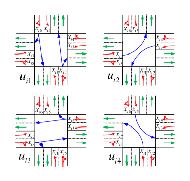
Figure 1: Four phases at a four-way intersection. Intersection $i$ has eight state variables including the number of vehicles $x_{i1},\ldots,x_{i8}$ and four control inputs $u_{i1},\ldots,u_{i4}$. Note that $x_{i1},x_{i5}$ are controlled by $u_{i4}$; $x_{i2},x_{i6}$ are controlled by $u_{i1}$; $x_{i3},x_{i7}$ are controlled by $u_{i2}$; $x_{i4},x_{i8}$ are controlled by $u_{i3}$.

2 Problem formulation

Consider a traffic network consisting of $N$ interconnected intersections. For ease of presentation, suppose that each intersection has eight roads connecting to it with vehicles moving in the same direction in each road as shown in Fig. 1. Each road has two lanes, where one lane is for vehicles going straight or turning right, and the other for left turn. A coupled system is used to model this traffic network, where each subsystem is comprised of one intersection and four roads with traffic streams entering it (the lanes with red arrows belong to subsystem $i$ and those with green arrows belong to its neighboring subsystems). Subsystem $i$ has a local state ${x_{i}}\in\mathbb{R}^{n}$ with $n=8$ and a local control input ${u_{i}}\in\mathbb{R}^{m}$ with $m=4$, where $x_{i1},\ldots,x_{i8}$ represent the number of vehicles in each lane entering this intersection and $u_{i1},\ldots,u_{i4}$ represent the green time for each phase to release vehicles, respectively.

The coupling relationship among the $N$ subsystems can be modeled by a directed graph $G=\left({V,E}\right)$, where the vertex set $V=\left\{{1,\ldots,N}\right\}$ represents the subsystems and the arc set $E\subseteq V\times V$ captures the coupling relationship among the subsystems. An arc $\left({j,i}\right)\in E$ means that there is a road connecting subsystem $j$ to $i$ and $j$ is regarded as a neighbor of $i$. Let ${\cal N}_{i}$ denote the set of neighbors of subsystem $i$ and let $|{N}_{i}|$ be the number of neighbors.

Note that the outflow of each subsystem can be controlled by setting the control input $u_{i}$, while the inflow of subsystem $i$ is uncontrollable by itself and is instead controlled by its neighboring subsystems, which is regarded as the interconnected influence. The dynamics of subsystem $i$ can be described as follows based on [8, 21, 22]

$${x_{i}}(k+1)={x_{i}}(k)-{B_{i}}(k){u_{i}}(k)+{C_{i}}(k){z_{i}}(k),\ i=1,\ldots,N,$$ (1)

where ${B_{i}}(k)\in\mathbb{R}^{n\times m}$ is the outflow rate of vehicles and can be measured by the road infrastructure, ${B_{i}}(k){u_{i}}(k)$ is the number of outflow vehicles of subsystem $i$ at time step $k$, ${C_{i}}(k)=\left[{{c_{{j_{1}}i}}(k),\ldots,{c_{{j_{l}}i}}(k),\ldots,{c_{{j_{|{\mathcal{N}_{i}}|}}i}}(k)}\right]\in\mathbb{R}^{n\times m|{\mathcal{N}_{i}}|}$, ${z_{i}}(k)={\left[{{u_{j_{1}}^{T}}(k),\ldots,{u_{j_{l}}^{T}}(k),\ldots,{u_{j_{|{\cal N}_{i}|}}^{T}(k)}}\right]^{T}}\in\mathbb{R}^{m|{\mathcal{N}_{i}}|},j_{l}\in{\cal N}_{i}$, ${C_{i}}(k){z_{i}}(k)=\sum\limits_{j_{l}\in{\cal N}_{i}}{{c_{j_{l}i}}}(k){u_{{j_{l}}}}(k)$ denotes the total number of vehicles that exit neighboring subsystems and enter subsystem $i$, ${u_{{j_{l}}}}(k),j_{l}\in{\cal N}_{i}$ is the control input of subsystem $j_{l}$, and ${{c_{j_{l}i}}}(k)$ is the transfer rate from subsystem $j_{l}$ to subsystem $i$. Since ${{c_{j_{l}i}}}(k),j_{l}\in{\cal N}_{i}$ comes from multiple directions, it is difficult to obtain in practice. Hence, ${{c_{j_{l}i}}}(k)$ and ${C_{i}}(k)$ are supposed unknown and will be estimated below in this paper.

Remark 1

For the case when a traffic network consists of roads that have more than two lanes, or intersections with more control phases, the traffic model can be similarly formulated and our discussions below apply as well.

The unbalanced traffic flow distribution is one of the main reasons that lead to traffic congestion. The vehicle density balancing idea is presented in traffic scenarios in [4, 3, 23], which tries to use the infrastructure evenly and avoid some overly congested lanes and some underutilized others. Achieving balanced vehicle density for all links at the same time is impractical for large-scale traffic networks due to the high dimensionality of the traffic network model, the complex coupling relationship between intersections, and so on.

In this paper, we aim to achieve local uniform vehicle density distribution for each link with the downstream links by designing the control input for each subsystem. The distributed MPC scheme is utilized below to assign the green times for each phase of traffic lights to avoid the congestion caused by uneven traffic flow distribution. When the distributed MPC scheme is implemented in a real-life large-scale traffic network, solving the distributed MPC optimization problem as fast as possible so as to apply the control signal timely is a big challenge [24]. This paper focuses on how to fast derive the solution of the distributed MPC optimization problem based on the proposed two-lane traffic model.

Remark 2

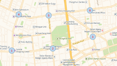
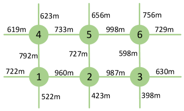
Figure 2: Part of a traffic network of Dalian City, China.

Note that in the traffic model in [25], the number of vehicles in a road is denoted by one state variable and then it is coupled with multiple control inputs, for example, when the number of vehicles denoted by $x_{i1}$ and $x_{i2}$ is represented by one variable $\bar{x}_{i1}$, then this state $\bar{x}_{i1}$ is controlled by two control inputs $u_{i1}$ and $u_{i4}$ in Fig. 2. The merit of the two-lane traffic model established in (1) is that it decouples the state variables and control inputs, which paves the way for making use of ADMM to design a fast algorithm for the optimal traffic light signals.

3 Distributed MPC scheme via ADMM

To determine the green times of each phase of all the intersections in a traffic network, we first review ADMM in this section, then the distributed MPC problem is formulated, and lastly, ADMM is utilized to fast obtain the solution of the distributed MPC problem.

3.1 Review of ADMM

ADMM solves the optimization problem of the following form:

$$\min\ \ f(x)+g(z),$$

$$\mathrm{s.\,t.}\ \ Ax+Bz=d,$$

where $x\in\mathbb{R}^{m},z\in\mathbb{R}^{n}$ are the control variables, $f\!:\!\mathbb{R}^{m}\!\to\!\mathbb{R},~{}g\!:\!\mathbb{R}^{n}\!\to\!\mathbb{R}$ are convex functions, and $A\in\mathbb{R}^{p\times m},B\in\mathbb{R}^{p\times n}$ and $d\in\mathbb{R}^{p}$. ADMM makes use of the dual ascent method with the following augmented Lagrangian

$${{\cal L}_{\rho}}(x,z,\lambda)=f(x)+g(z)+{\lambda^{T}}(Ax+Bz-d)+\frac{1}{2}\left\|{Ax+Bz-d}\right\|_{2}^{2},$$

where $\lambda$ is the Lagrange multiplier, and $\rho$ is a positive constant to accelerate the convergence of the algorithm. In ADMM, the variables are updated by iteratively minimizing ${{\cal L}_{\rho}}(x,z,\lambda)$ with respect to $x$ and $z$, and the iterations are given by

$$x^{k+1} =\arg\mathop{\min}\limits_{x}{{\cal L}_{\rho}}(x,z^{k},\lambda^{k}),$$

$$z^{k+1} =\arg\mathop{\min}\limits_{z}{{\cal L}_{\rho}}(x^{k+1},z,\lambda^{k}),$$

$$\lambda^{k+1} =\lambda^{k}+\rho(Ax^{k+1}+Bz^{k+1}-d).$$

To monitor the convergence of the algorithm towards optimality, the primal residuals $r^{k}$ and dual residuals $s^{k}$ of iteration $k$ are defined as

$$r^{k+1} =Ax^{k+1}+Bz^{k+1}-d,$$

$$s^{k+1} =\rho A^{T}B(z^{k+1}-z^{k}).$$

The stopping criterion is that the primal residuals $r^{k}$ and dual residuals $s^{k}$ are less than some predefined small thresholds. The number of iterations is also utilized as a stopping criterion especially when an approximate solution is desirable. For more details on the stopping criterion and convergence analysis of ADMM, one can refer to [26].

3.2 Distributed MPC framework

To employ distributed MPC scheme, the $M$-step ahead equation (2) below can be obtained from (1)

$$\begin{cases}{x_{i}}(k+1)&={x_{i}}(k)-{B_{i}}(k){u_{i}}(k)+{C_{i}}(k){z_{i}}(k),\\ {x_{i}}(k+2)&={x_{i}}(k+1)-{B_{i}}(k+1){u_{i}}(k+1)+{C_{i}}(k+1){z_{i}}(k+1)\\ &={x_{i}}(k)-{B_{i}}(k){u_{i}}(k)+{C_{i}}(k){z_{i}}(k)-{B_{i}}(k+1){u_{i}}(k+1)+{C_{i}}(k+1){z_{i}}(k+1),\\ &\ \vdots\\ {x_{i}}(k+M)&={x_{i}}(k+M-1)-{B_{i}}(k+M-1){u_{i}}(k+M-1)+{C_{i}}(k+M-1){z_{i}}(k+M-1)\\ &={x_{i}}(k+M-2)-{B_{i}}(k+M-2){u_{i}}(k+M-2)+{C_{i}}(k+M-2){z_{i}}(k+M-2)\\ &\ \ \ -{B_{i}}(k+M-1){u_{i}}(k+M-1)+{C_{i}}(k+M-1){z_{i}}(k+M-1)\\ &\ \vdots\\ &={x_{i}}(k)-\sum\limits_{j=0}^{M-1}{{B_{i}}(k+j){u_{i}}(k+j)}+\sum\limits_{j=0}^{M-1}{{C_{i}}(k+j){z_{i}}(k+j)}.\end{cases}$$ (2)

Then, equation (2) can be rewritten into a compact form

$${{y_{i}}(k+1)}=E\otimes{x_{i}}(k)-{{\mathcal{B}_{i}}}(k)U_{i}(k)+{{\mathcal{C}_{i}}}(k)Z_{i}(k),$$

with

$${y_{i}}(k+1)={\left[{{x_{i}^{T}}(k+1),\ldots,{x_{i}^{T}}(k+M)}\right]^{T}},$$

$${{\mathcal{B}_{i}}}(k)=\left[{\begin{array}[]{*{20}{c}}{{B_{i}}(k)}&\bm{0}&\cdots&\bm{0}\\ {{B_{i}}(k)}&{{B_{i}}(k+1)}&\cdots&\bm{0}\\ \vdots&\vdots&\ddots&\bm{0}\\ {{B_{i}}(k)}&{{B_{i}}(k+1)}&\cdots&{{B_{i}}(k+M-1)}\end{array}}\right],$$ (7)

$${{\mathcal{C}_{i}}}(k)=\left[{\begin{array}[]{*{20}{c}}{{C_{i}}(k)}&\bm{0}&\cdots&\bm{0}\\ {{C_{i}}(k)}&{{C_{i}}(k+1)}&\cdots&\bm{0}\\ \vdots&\vdots&\ddots&\bm{0}\\ {{C_{i}}(k)}&{{C_{i}}(k+1)}&\cdots&{{C_{i}}(k+M-1)}\end{array}}\right],$$ (12)

$${U_{i}}(k)={\left[{{u_{i}^{T}}(k),\ldots,{u_{i}^{T}}(k+M-1)}\right]^{T}},$$

$${Z_{i}}(k)={\left[{{z_{i}^{T}}(k),\ldots,{z_{i}^{T}}(k+M-1)}\right]^{T}},$$

$$E=\bm{1}_{M},$$

where $\bm{1}_{M}$ is the $M$-dimensional column vector whose entries all equal 1, and $\otimes$ is the Kronecker product. Note that the matrix ${{\mathcal{C}}_{i}}(k)$ in (12) is unknown, and ${C_{i}}(k)$ can be estimated and forecasted by minimizing the following cost function [27]

$$J({C_{i}}(k))=\big{\|}{x_{i}}(k)-{x_{i}}(k-1)+{B_{i}}(k-1){u_{i}}(k-1)-{C_{i}}(k){z_{i}}(k-1)\big{\|}_{2}^{2}+{\mu_{i}}\big{\|}{{C_{i}}(k)-{{\hat{C}}_{i}}(k-1)}\big{\|}_{2}^{2},$$ (13)

where ${{\hat{C}}_{i}}(k-1)$ is the estimate of ${C_{i}}(k-1)$, $\mu_{i}>0$ is a weighting factor to restrain the exaggerated change of pseudogradients, and ${\left\|x\right\|_{2}}$ denotes the 2-norm of a vector $x$. Then, the estimate ${{\hat{C}}_{i}}(k)$ can be updated by minimizing (13) with respect to ${C_{i}}(k)$ as

$${{\hat{C}}_{i}}(k)= {{\hat{C}}_{i}}(k-1)+({x_{i}}(k)-{x_{i}}(k-1)+{B_{i}}(k-1){u_{i}}(k-1)-{{\hat{C}}_{i}}(k-1){z_{i}}(k-1)){z_{i}}^{T}(k-1)$$

$$\times{({\mu_{i}}I_{{m|{\mathcal{N}_{i}}|}}+{z_{i}}(k-1){z_{i}}^{T}(k-1))^{-1}},$$ (14)

where $I_{{m|{\mathcal{N}_{i}}|}}$ is the ${{m|{\mathcal{N}_{i}}|}}$ dimensional identity matrix. Unfortunately, the estimation method above cannot be used to get the estimates of ${B_{i}(k+1)},\ldots,{B_{i}(k+M-1)}$ in ${\mathcal{B}_{i}}(k)$, and the estimates of ${C_{i}(k+1)},\ldots,{C_{i}(k+M-1)}$ in ${\mathcal{C}_{i}}(k)$ directly. Since there are many zero elements in matrices ${\mathcal{B}_{i}}(k)$ and ${\mathcal{C}_{i}}(k)$, we append the nonzero elements of ${B_{i}(k+1)},\ldots,{B_{i}(k+M-1)}$, ${C_{i}(k+1)},\dots,{C_{i}(k+M-1)}$ into vectors ${b_{i}(k+1)},\dots,$ ${b_{i}(k+M-1)}$, ${c_{i}(k+1)},\dots,$ ${c_{i}(k+M-1)}$, respectively. A multi-layer hierarchical forecasting method is employed in this paper to forecast these variables, and one has

$${{\hat{b}}_{i}}(k+j)= {\varphi_{1}}(k){{\hat{b}}_{i}}(k+j-1)+{\varphi_{2}}(k){{\hat{b}}_{i}}(k+j-2)+\cdots+{\varphi_{p}}(k){{\hat{b}}_{i}}(k+j-p),$$ (15)

$${{\hat{c}}_{i}}(k+j)= \ {\theta_{1}}(k){{\hat{c}}_{i}}(k+j-1)+{\theta_{2}}(k){{\hat{c}}_{i}}(k+j-2)+\cdots+{\theta_{p}}(k){{\hat{c}}_{i}}(k+j-p),$$ (16)

where ${{\hat{b}}_{i}}(k),{{\hat{c}}_{i}}(k)$ are the estimates of ${b_{i}}(k)$, ${c_{i}}(k)$, respectively, $j=1,\ldots,M-1,$ and $p$ is an appropriate order and normally set as 2-7 [28, 29].

Then, let ${\varphi(k)}\buildrel\Delta\over{=}\left[{{\varphi_{1}}(k),\ldots,{\varphi_{p}}(k)}\right]^{T}$, ${\theta(k)}\buildrel\Delta\over{=}\left[{{\theta_{1}}(k),\ldots,{\theta_{p}}(k)}\right]^{T}$, which can be updated as follows [28]

$${\varphi(k)}= {\varphi(k-1)}+\frac{{\hat{\eta}_{i}(k-1)}}{{\delta+{{\left\|{{{\hat{\eta}}_{i}}(k-1)}\right\|}_{2}}}}\times\left[{{{\hat{b}}_{i}}(k)-{{\hat{\eta}}_{i}}^{T}(k-1){\varphi(k-1)}}\right],$$ (17)

$${\theta(k)}= {\theta(k-1)}+\frac{{\hat{\Xi}_{i}(k-1)}}{{\delta+{{\left\|{{{\hat{\Xi}}_{i}}(k-1)}\right\|}_{2}}}}\times\left[{{{\hat{c}}_{i}}(k)-{{\hat{\Xi}}_{i}}^{T}(k-1){\theta(k-1)}}\right],$$ (18)

where ${{\hat{\eta}}_{i}}(k-1)=\left[{{{\hat{b}}_{i}}(k-1),\ldots,{{\hat{b}}_{i}}(k-p)}\right]^{T}$, ${{\hat{\Xi}}_{i}}(k-1)=\left[{{{\hat{c}}_{i}}(k-1),\ldots,{{\hat{c}}_{i}}(k-p)}\right]^{T}$, and $\delta\in\left({0,1}\right]$ is employed to avoid that the denominator equals to zero.

3.3 Distributed traffic signal control via ADMM

To realize the objective of achieving local uniform vehicle density distribution for each link with the downstream links [4, 3, 21], the cost function of the entire network can be formulated as follows

$$\min\sum\limits_{i=1}^{N}{{\phi_{i}}(k)}=\sum\limits_{i=1}^{N}{\left({\sum\limits_{m=1}^{8}{\sum\limits_{h=1}^{M}{{{\left({{\rho_{im}}(k+h)-{{\bar{\rho}}_{im}}(k+h)}\right)}^{2}}}}}\right.} \left.{+{\sum\limits_{h=1}^{M-1}{{u_{i}^{T}}}(k+h)}{R_{i}}{u_{i}}(k+h)}\right),$$ (19a)

$$\mathrm{s.\,t.}\ \ \ {x_{i}}(k+1)={x_{i}}(k)-{B_{i}}(k){u_{i}}(k)+{C_{i}}(k){z_{i}}(k),$$ (19b)

$${\bar{\rho}}_{im}(k+h)=\frac{1}{{|N_{im}^{+}{\rm{|}}}}{\sum\limits_{jg\in N_{im}^{+}}{{x_{jg}}(k+h)/{L_{jg}}}},h=1,\ldots,M,$$ (19c)

$$\sum\limits_{m=1}^{4}{{u_{im}}}(k+h)+{Q_{i}}=S,\ \ h=1,\ldots,M-1,$$ (19d)

$${u_{im}}(k+h)\in\left[{{u_{\min}},{u_{\max}}}\right],\ \ h=1,\ldots,M-1,$$ (19e)

where $x_{im}(k)$ and $u_{im}(k)$ are the $m$th elements of $x_{i}(k),u_{i}(k)$, respectively, ${\bar{\rho}}_{im}(k+h)$ is the average vehicle density of the downstream links of $im$ at predictive step $h$, $L_{im}$ is the length of link $im$ and $L_{jg}$ is defined similarly, $N_{im}^{+}$ denotes the set of the downstream links of $im$ that have traffic flowing directly from $im$, $|{N_{im}^{+}{\rm{|}}}$ denotes the number of downstream links of link $im$, ${R_{i}}=diag\left({{r_{i1}},{r_{i2}},{r_{i3}},{r_{i4}}}\right)$ is a diagonal positive definite matrix such that the two items in (19a) are of the same order of magnitude, $Q_{i}$ is the yellow light time at subsystem $i$ and keeps unchanged during the optimization process, $S$ is the cycle length of traffic lights and assumed to be the same for all intersections, and ${u_{\min}}$ and ${u_{\max}}$ are the minimum and maximum green times for ${u_{im}}(k+h)$. The first term in (19a) is to minimize the difference between the vehicle density of each link and the average vehicle density of the downstream links, and the second term is a regularization term to accelerate the convergence of the optimization problem.

By solving the optimization problem (19a) with constraints (19b)-(19e), one can derive the green time of each phase of all the intersections with the optimal performance for the entire network. However, the centralized optimization method involves massive data transmission and has high online computational complexity, which is impractical for multiple interconnected intersections. From the above analysis, an intersection belongs to only one subsystem after the traffic system decomposition. Hence, a distributed optimization framework for urban traffic signals is proposed. The optimization problem for each subsystem is presented as follows

$$\min{\phi_{i}}(k){\rm{}}=\sum\limits_{m=1}^{8}{\sum\limits_{h=1}^{M}{{{\left({{\rho_{im}}(k+h)-{{\bar{\rho}}_{im}}(k+h)}\right)}^{2}}}}+{\sum\limits_{h=1}^{M-1}{{u_{i}}^{T}{(k)}}}{R_{i}}{u_{i}}(k),\ i=1,\ldots,N,$$ (20)

$\mathrm{s.\,t.}\ \ \ (\ref{st1})-(\ref{st2})$.

Although the optimization problem of the whole network (19a) is transformed into a distributed optimization framework (20) based on the system decomposition, it is still hard to apply in real-life traffic networks since the computational speed of solving (20) with constraints (19b)-(19e) directly may not meet practical traffic control requirements [15, 24]. Since the state variables and control inputs are decoupled in the proposed two-lane traffic model, one can split the optimization problem (20) into several subproblems. Then, the distributed MPC problem (20) can be rewritten in the following form

$$\min{\phi_{i}}(k)=\min\sum\limits_{m=1}^{4}{{f_{im}}}(U_{im}(k)),\ i=1,\ldots,N,$$ (21a)

where

$${f_{i1}}(U_{i1}(k))= \sum\limits_{m=2,6}{\sum\limits_{h=1}^{M}{{{\left({{\rho_{im}}(k+h)-{{\bar{\rho}}_{im}}(k+h)}\right)}^{2}}}}+{{U_{i1}^{T}}(k)}{r_{i1}}{U_{i1}}(k),$$ (21b)

$${f_{i2}}(U_{i2}(k))= \sum\limits_{m=3,7}{\sum\limits_{h=1}^{M}{{{\left({{\rho_{im}}(k+h)-{{\bar{\rho}}_{im}}(k+h)}\right)}^{2}}}}+{{U_{i2}^{T}}(k)}{r_{i2}}{U_{i2}}(k),$$ (21c)

$${f_{i3}}(U_{i3}(k))= \sum\limits_{m=4,8}{\sum\limits_{h=1}^{M}{{{\left({{\rho_{im}}(k+h)-{{\bar{\rho}}_{im}}(k+h)}\right)}^{2}}}}+{{U_{i3}^{T}}(k)}{r_{i3}}{U_{i3}}(k),$$ (21d)

$${f_{i3}}(U_{i4}(k))= \sum\limits_{m=1,5}{\sum\limits_{h=1}^{M}{{{\left({{\rho_{im}}(k+h)-{{\bar{\rho}}_{im}}(k+h)}\right)}^{2}}}}+{{U_{i4}^{T}}(k)}{r_{i4}}{U_{i4}}(k),$$ (21e)

$\mathrm{s.\,t.}\ \ \ (\ref{st1})-(\ref{st2})$,
where ${U_{im}}(k)={\left[{{u_{im}^{T}}(k),\ldots,{u_{im}^{T}}(k+M-1)}\right]^{T}},m=1,2,3,4$, $r_{im}$ is the $m$th diagonal element of $R_{i}$. Since ADMM has superior stability properties and decomposability in solving optimization problems with constraints, it is employed in this paper to solve (21a) with constraints (19b)-(19e) to obtain the optimal design of traffic lights in urban traffic networks. The detailed procedure of the algorithm at each time step $k$ is summarized in Algorithm 1.

Algorithm 1 Distributed Traffic Signal Control for Urban Traffic Networks via ADMM

Input: Maximum computation time $T_{max}$; iteration stop threshold $\varepsilon_{stop}$
Output: Control inputs $U_{i}(k)$
1: For $i=1,2,\dots,N$ in a parallel fashion do
2:  Initialization: Iteration index $s\leftarrow 1$, total computation time $t_{i}(k)\leftarrow 0$, measure the number of vehicles $x_{i}(k)$
3:  Whlie $\varepsilon^{s}\geq\varepsilon_{stop}$ and $t_{i}(k)\leq T_{max}$
4:    Receive ${{U}}_{j}(k-1),{{{y}}_{j}(k-1)}$ from neighboring subsystems
5:    Update the system parameters $\mathcal{B}_{i}(k)$ and $\mathcal{C}_{i}(k)$ according to (13)-(18)
6:    Solve the following optimization problem

$$\qquad\qquad\qquad\min{\cal L}_{\rho}(U_{i1}(k),U_{i2}(k),U_{i3}(k),U_{i4}(k),\lambda)\mathop{=}\left({\sum\limits_{m=1}^{4}{{f_{im}}({U_{im}}(k))}+\frac{\rho}{2}{{\left\|{\vartheta(k)}\right\|}^{2}}+{\lambda^{T}}\vartheta(k)}\right)$$

    where ${\vartheta(k)}=\vartheta({U_{i1}}(k),{U_{i2}}(k),{U_{i3}}(k),{U_{i4}}(k))=\left[{\begin{array}[]{*{20}{c}}{\sum\limits_{m=1}^{4}{{u_{im}}(k+1)}+{Q_{i}}-S}\\ {\sum\limits_{m=1}^{4}{{u_{im}}(k+2)}+{Q_{i}}-S}\\ \vdots\\ {\sum\limits_{m=1}^{4}{{u_{im}}(k+M-1)}+{Q_{i}}-S}\end{array}}\right],\lambda={\left[{{\lambda_{1}},\ldots,{\lambda_{M-1}}}\right]^{T}}$
7:    Update

$$\qquad\qquad\qquad{U_{i1}}^{(s)}(k) =\mathop{\arg\min}\limits_{{}_{{U_{i1}}}(k)}\big{(}{\cal L}_{\rho}({U_{i1}}(k),U_{i2}^{(s-1)}(k),U_{i3}^{(s-1)}(k),U_{i4}^{(s-1)}(k)),{\lambda^{(s-1)}}\big{)}$$

$${U_{i2}}^{(s)}(k) =\mathop{\arg\min}\limits_{{}_{{U_{i2}}}(k)}\big{(}{\cal L}_{\rho}(U_{i1}^{(s)}(k),{U_{i2}}(k),U_{i3}^{(s-1)}(k),U_{i4}^{(s-1)}(k)),{\lambda^{(s-1)}}\big{)}$$

$${U_{i3}}^{(s)}(k) =\mathop{\arg\min}\limits_{{}_{{U_{i3}}}(k)}\big{(}{\cal L}_{\rho}(U_{i1}^{(s)}(k),U_{i2}^{(s)}(k),{U_{i3}}(k),U_{i4}^{(s-1)}(k)),{\lambda^{(s-1)}}\big{)}$$

$${U_{i4}}^{(s)}(k) =\mathop{\arg\min}\limits_{{}_{{U_{i4}}}(k)}\big{(}{\cal L}_{\rho}(U_{i1}^{(s)}(k),U_{i2}^{(s)}(k),U_{i2}^{(s)}(k),{U_{i4}}(k)),{\lambda^{(s-1)}}\big{)}$$

$${\lambda^{(s)}} ={\lambda^{(s-1)}}+\rho\vartheta\big{(}{U_{i1}}^{(s)}(k),{U_{i2}}^{(s)}(k),{U_{i3}}^{(s)}(k),{U_{i4}}^{(s)}(k)\big{)}$$

8:    Update the computation time $t_{i}(k)$
9:    Compute ${\varepsilon^{s+1}}\leftarrow{\left\|{{\lambda^{(s)}}-\vartheta\big{(}{U_{i1}}^{(s)}(k),{U_{i2}}^{(s)}(k),{U_{i3}}^{(s)}(k),{U_{i4}}^{(s)}(k)\big{)}}\right\|_{\infty}}$
10:    $s\leftarrow s+1$
11:    Send ${U}_{i}(k),{{{y}}_{i}(k)}$ to neighboring subsystems
12:  End While
13: End For

At every time step, each subsystem solves its optimization problem with constraints (19b)-(19e) based on Algorithm 1 by receiving the information of neighboring subsystems. Then, it shares the intermediate solution with its neighboring subsystems to solve their optimization problems with the received information. Finally, all the control inputs $U_{i}(k),i=1,2,\ldots,N$ of the whole network are obtained, and applying the first control of $U_{i}(k)$ on subsystem $i$.

4 Case study

To evaluate the effectiveness of the proposed two-lane traffic model and the distributed MPC scheme, a six-intersection traffic network with 68 roads from Dalian city, China as shown in Fig. 3 is considered. The network is simulated using VISSIM with control algorithms programmed in PYTHON. The sampling period and the common cycle length of all intersections are set as $S$ = 120 s, and the total simulation time is 7200 s, which corresponds to 60 control intervals. The scenarios of the experiment mimic the morning rush hour of Dalian, and the traffic demand of each link varies from 300 to 800 vehicles per hour. For each phase, the lower bound $u_{min}$ and upper bound $u_{max}$ are set as 10s and 70s, respectively, and the prediction horizon is set to $M$ = 5. By contrasting the proposed distributed MPC scheme based on ADMM (MPC-ADMM) with fixed-time control (FTC), distributed MPC scheme solving by PYTHON packet (MPC-PYTHON), distributed MPC scheme for the road-based model (MPC-ROAD), the effectiveness and nice performance of the proposed strategy are shown.

1. [1)]

2. FTC indicates that each intersection uses the fixed signal timing scheme [5] i.e., each phase accounts for a quarter of the cycle time in this paper.

3. MPC-PYTHON means to solve the distributed MPC problem by PYTHON packet, which is utilized to compare the computing speed with our proposed method.

4. To show the superiority of the proposed two-lane traffic model, the MPC-ROAD [8] is compared in this paper, which implies using the MPC scheme to assign the green time of each phase based on the road modeling.

To compare the performance of the control strategies, three criteria, including the average density, the average flow rate, and the relative loss time, are compared. The average density is the average of density of all vehicles on the roads, and a low average density indicates that there is generally less congestion and more throughput in the network. In addition, the average flow rate implies the network’s traffic situation through quantities such as the total delay time of vehicles, the average travel speed, the throughput of the network and so on. The relative loss time means time lost per second by vehicles relative to free-flowing vehicles, which is an essential indicator to reveal the traffic congestion of the network. A thorough analysis of all the above criteria can be used to evaluate the traffic situation.

To evaluate the effect of traffic light control more intuitively, the average density of the network, the average speed, and the relative loss time under different control strategies are shown in Figs. 3-5, and the rest four performance indices including the average delay, average number of stops, total travel time, and average computing time are calculated in Table 1. These performance indices can be obtained directly from VISSIM simulation software. Table 1 and Figs. 3-5 demonstrate that MPC-ADMM has the best control effects because it has the smallest average delay, average number of stops, total travel time, and average computing time. MPC-ADMM and MPC-PHTHON have comparable control performance and better control effects than FTC and MPC-ROAD, but MPC-ADMM consumes less average computation time.

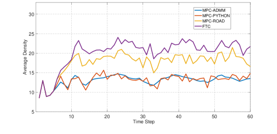
Figure 3: The average density of vehicles on the roads under different control strategies.

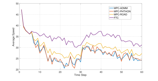
Figure 4: The average speed of vehicles on the roads under different control strategies.

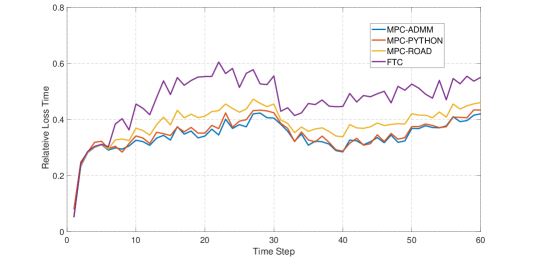
Figure 5: The relative loss time under different control strategies.

Table 1: The performance indexes under different control strategies.

Control strategy	Average delay [s]	Average stops	Total travel time [h]	Average computation time [s]
MPC-ADMM	105.164	3.129	937.502	1.323
MPC-PHTHON	106.468	3.154	941.562	4.137
MPC-ROAD	164.235	5.264	1089.354	4.389
FTC	229.500	8.858	1345.288	/

5 Conclusion

In this paper, a novel two-lane traffic model was proposed for traffic signal control by looking into the number of vehicles in multiple lanes with different destinations. Different from traditional technologies to model urban traffic networks based on roads, the proposed lane-based traffic model provides a practical version to better model traffic flow propagation. The distributed MPC scheme was employed to derive the green times of each phase at intersections. To meet the real-time feasibility requirement when applying the distributed MPC scheme, ADMM was utilized based on the proposed two-lane traffic model. Simulation results illustrated the feasibility and effectiveness of the proposed method. For future work, we will look into the two-level hierarchical control scheme for large-scale traffic networks.

Declaration of competing interest

The authors declare that they have no known competing financial interests or personal relationships that could have appeared to influence the work reported in this paper.

References

- [1] G. De Nunzio, G. Gomes, C. C. de Wit, R. Horowitz, P. Moulin, Arterial bandwidth maximization via signal offsets and variable speed limits control, in: 2015 54th IEEE Conference on Decision and Control (CDC), IEEE, 2015, pp. 5142–5148.
- [2] Q. Ba, K. Savla, G. Como, Distributed optimal equilibrium selection for traffic flow over networks, in: 2015 54th IEEE Conference on Decision and Control (CDC), IEEE, 2015, pp. 6942–6947.
- [3] P. Grandinetti, C. Canudas-de Wit, F. Garin, Distributed optimal traffic lights design for large-scale urban networks, IEEE Transactions on Control Systems Technology 27 (3) (2018) 950–963.
- [4] X. Ru, C. Mei, W. Xia, P. Shi, Distributed model-free adaptive predictive control of traffic lights for multiple interconnected intersections, SCIENCE CHINA Information Sciences 66 (9) (2023) 190209.
- [5] D. I. Robertson, Transyt method for area traffic control, Traffic Engineering & Control 8 (8) (1969).
- [6] D. I. Robertson, R. D. Bretherton, Optimizing networks of traffic signals in real time-the scoot method, IEEE Transactions on Vehicular Technology 40 (1) (1991) 11–15.
- [7] A. G. Sims, K. W. Dobinson, The sydney coordinated adaptive traffic (scat) system philosophy and benefits, IEEE Transactions on vehicular technology 29 (2) (1980) 130–137.
- [8] E. Camponogara, L. B. De Oliveira, Distributed optimization for model predictive control of linear-dynamic networks, IEEE Transactions on Systems, Man, and Cybernetics-Part A: Systems and Humans 39 (6) (2009) 1331–1338.
- [9] F. Motawej, R. Bouyekhf, A. El Moudni, A dissipativity-based approach to traffic signal control for an over-saturated intersection, Journal of the Franklin Institute 348 (4) (2011) 703–717.
- [10] A. A. Zaidi, B. Kulcsár, H. Wymeersch, Back-pressure traffic signal control with fixed and adaptive routing for urban vehicular networks, IEEE Transactions on Intelligent Transportation Systems 17 (8) (2016) 2134–2143.
- [11] Z. Su, A. H. Chow, R. Zhong, Adaptive network traffic control with an integrated model-based and data-driven approach and a decentralised solution method, Transportation Research Part C: Emerging Technologies 128 (2021) 103154.
- [12] F. Yan, F. Tian, Z. Shi, An extended signal control strategy for urban network traffic flow, Physica A: Statistical Mechanics and its Applications 445 (2016) 117–127.
- [13] T. Zhang, P. Shi, W. Li, X. Yue, Ekf enhanced mpc for rapid attitude stabilization of space robots with bounded control torque in postcapture, Journal of the Franklin Institute 360 (11) (2023) 7105–7127.
- [14] Q. Lu, P. Shi, J. Liu, L. Wu, Model predictive control under event-triggered communication scheme for nonlinear networked systems, Journal of the Franklin Institute 356 (5) (2019) 2625–2644.
- [15] S. Lin, B. De Schutter, Y. Xi, H. Hellendoorn, Fast model predictive control for urban road networks via milp, IEEE Transactions on Intelligent Transportation Systems 12 (3) (2011) 846–856.
- [16] B.-L. Ye, W. Wu, K. Ruan, L. Li, T. Chen, H. Gao, Y. Chen, A survey of model predictive control methods for traffic signal control, IEEE/CAA Journal of Automatica Sinica 6 (3) (2019) 623–640.
- [17] T. Bai, S. Li, Y. Zheng, Distributed model predictive control for networked plant-wide systems with neighborhood cooperation, IEEE/CAA Journal of Automatica Sinica 6 (1) (2019) 108–117.
- [18] S. Boyd, N. Parikh, E. Chu, B. Peleato, J. Eckstein, et al., Distributed optimization and statistical learning via the alternating direction method of multipliers, Foundations and Trends® in Machine learning 3 (1) (2011) 1–122.
- [19] T. Bai, S. Li, Y. Zou, Distributed mpc for reconfigurable architecture systems via alternating direction method of multipliers, IEEE/CAA Journal of Automatica Sinica 8 (7) (2020) 1336–1344.
- [20] A. Mishra, U. K. Sahoo, S. Maity, Sparsity promoting decentralized learning strategies for radio tomographic imaging using consensus based admm approach, Journal of the Franklin Institute 360 (7) (2023) 5211–5241.
- [21] N. Wu, D. Li, Y. Xi, Balance traffic control in urban traffic networks based on distributed optimization, in: 2016 IEEE 19th International Conference on Intelligent Transportation Systems (ITSC), IEEE, 2016, pp. 428–433.
- [22] N. Wu, D. Li, Y. Xi, Distributed integrated control of a mixed traffic network with urban and freeway networks, IEEE Transactions on Control Systems Technology 30 (1) (2021) 57–70.
- [23] N. Wu, D. Li, Y. Xi, Balance traffic control in urban traffic networks based on distributed optimization, in: 2016 IEEE 19th International Conference on Intelligent Transportation Systems (ITSC), IEEE, 2016, pp. 428–433.
- [24] F. Farokhi, I. Shames, K. H. Johansson, Distributed mpc via dual decomposition and alternative direction method of multipliers, in: Distributed model predictive control made easy, Springer, 2013, pp. 115–131.
- [25] G. Bianchin, F. Pasqualetti, Gramian-based optimization for the analysis and control of traffic networks, IEEE Transactions on Intelligent Transportation Systems 21 (7) (2019) 3013–3024.
- [26] S. Boyd, N. Parikh, E. Chu, B. Peleato, J. Eckstein, et al., Distributed optimization and statistical learning via the alternating direction method of multipliers, Foundations and Trends® in Machine learning 3 (1) (2011) 1–122.
- [27] Z. Hou, R. Chi, H. Gao, An overview of dynamic-linearization-based data-driven control and applications, IEEE Transactions on Industrial Electronics 64 (5) (2016) 4076–4090.
- [28] D. Li, B. De Schutter, Distributed model-free adaptive predictive control for urban traffic networks, IEEE Transactions on Control Systems Technology 30 (1) (2021) 180–192.
- [29] Z. Hou, S. Jin, Model free adaptive control, CRC press Boca Raton, FL, 2013.