Angular velocity and linear acceleration measurement bias estimators for the rigid body system with global exponential convergence

Soham Shanbhag sshanbhag@kaist.ac.kr School of Electrical Engineering, Korea Advanced Institute of Science and Technology, Daejeon, Republic of Korea Dong Eui Chang Corresponding author, dechang@kaist.ac.kr School of Electrical Engineering, Korea Advanced Institute of Science and Technology, Daejeon, Republic of Korea
Abstract

Rigid body systems usually consider measurements of the pose of the body using onboard cameras/LiDAR systems, that of linear acceleration using an accelerometer and of angular velocity using an IMU. However, the measurements of the linear acceleration and angular velocity are usually biased with an unknown constant or slowly varying bias. We propose a measurement bias estimator for such systems under assumption of boundedness of angular velocity. We also provide continuous estimates to the state of the system, i.e. the pose, linear velocity, and position of the body. These estimates are globally exponentially convergent to the state of the rigid body system. We propose two bias estimators designed with the estimate of the pose in the ambient Euclidean space of the Special Euclidean group and show global exponential convergence of the proposed observers to the state of the system. The first observer assumes knowledge of bounds of the angular velocity, while the second observer uses a Riccati observer to overcome this limitation. We show the convergence with an example of a rigid body rotation and translation system on the special Euclidean group. We show that the observer is able to estimate the bias using data collected from an Intel Realsense camera.

1 Introduction

Research in quadcopter design and control has been increasing due to their use in military and civilian applications[2]. For effective use of these systems, the study of control of these systems is paramount. However, for feedback based control, one important design consideration is the integration of sensors in those systems for providing the state of the system. Sensors proposed for this quadcopter system usually measure the position of various landmarks in the environment, given by the equation

yi=RT​(piβˆ’p),subscript𝑦𝑖superscript𝑅𝑇subscript𝑝𝑖𝑝\displaystyle y_{i}=R^{T}(p_{i}-p),

where R𝑅R is the matrix denoting the rotation of the quadcopter frame with respect to the ground frame, p𝑝p is the position of the quadcopter in the ground frame, and pisubscript𝑝𝑖p_{i}s and yisubscript𝑦𝑖y_{i}s are the position of the landmarks in the ground and quadcopter frame, respectively. Moreover, measurements concerning angular velocity are collected using an IMU and linear velocity measurements are collected using GPS sensors or Doppler velocity sensors[5, 15, 14]. These problems are known as β€œAttitude and Heading Reference System” problems in the literature[8]. However, the measurement of linear velocity is difficult if velocity measurements are not available, like in GPS denied environments. Alternatively, accelerometer measurements have been also exploited as an alternative to linear velocity measurements due to their ease of use.

Usually, IMU and accelerometer sensor measurements are corrupted with a constant bias. Deterministic observers for state and bias estimation have been designed to estimate this bias in an online fashion. The authors in [9] design an almost semi-globally uniformly ultimately bounded observer for this system. The authors in [7] and [10] propose locally exponentially stable observers using the continuous Riccati equation. The authors in [1] propose an asymptotically stable observer using invariant extended Kalman filters. The authors in [3] propose a globally convergent observer for the bias in the accelerometer readings, but assume unbiased angular velocity measurements.

As can be seen, the observers proposed are unable to achieve global convergence in the presence of IMU and accelerometer bias. This is due to a topological obstruction on SO​(3)SO3\textrm{SO}(3) not allowing global observers[4]. Two methods are used to overcome this obstruction. The authors in [16] design a globally exponentially stable observer for the rigid body system. They design a hybrid (continuous + discrete) observer for the rigid body system with the state consisting of the rotational pose, translation pose, and the linear velocity. To the best of our knowledge, this is the first observer proposing global exponential stability. However, the hybrid nature of the observer leads to discontinuities in the observer dynamics, specifically the pose. Since the estimate of the pose is used in classical control methods, a discontinuity in the estimate of the pose is undesirable. Another alternative is the extension of the dynamics to the ambient Euclidean space. This approach has been used to solve similar problems, for example in [6, 12]. We use this approach to design globally convergent continuous observers for the rigid body system. An observer using a similar approach has been designed for the system considering linear velocity measurements instead of linear acceleration measurements in [13].

The ambient space extension allows us to design deterministic observers which are continuous and globally convergent. We propose two observers for this purpose. The first observer assumes knowledge of bounds of the angular velocity and proposes a constant gain observer. The second observer is a Riccati based variable gain observer, which is computationally expensive but assumes only the existence of a bound on the angular velocity, and no knowledge of the said bound. To our knowledge, these are the first observers able to provide global exponential convergence without discontinuities.

2 Preliminaries

We denote the estimate of the state A𝐴A by A¯¯𝐴\bar{A}. Denote by SO​(3)SO3\textrm{SO}(3) the set of orthogonal matrices of dimension 3 with determinant 1, and by 𝔰​𝔬​(3)𝔰𝔬3\mathfrak{so}(3) the corresponding Lie algebra. The elements of 𝔰​𝔬​(3)𝔰𝔬3\mathfrak{so}(3) are skew symmetric matrices in ℝ3Γ—3superscriptℝ33\mathbb{R}^{3\times 3}. The matrix representation of the cross product with a vector v𝑣v is denoted by vΓ—:ℝ3→𝔰​𝔬​(3):subscript𝑣→superscriptℝ3𝔰𝔬3v_{\times}:\mathbb{R}^{3}\to\mathfrak{so}(3) such that for all wβˆˆβ„3,vΓ—w=v×​wformulae-sequence𝑀superscriptℝ3𝑣𝑀subscript𝑣𝑀w\in\mathbb{R}^{3},v\times w=v_{\times}w. The inverse of the (β‹…)Γ—subscriptβ‹…(\cdot)_{\times} operator is denoted by (β‹…)∨:𝔰​𝔬​(3)→ℝ3:subscript⋅→𝔰𝔬3superscriptℝ3(\cdot)_{\vee}:\mathfrak{so}(3)\to\mathbb{R}^{3}, where for all aβˆˆβ„3,(aΓ—)∨=aformulae-sequenceπ‘Žsuperscriptℝ3subscriptsubscriptπ‘Žπ‘Ža\in\mathbb{R}^{3},(a_{\times})_{\vee}=a and for all Aβˆˆπ”°β€‹π”¬β€‹(3),(A∨)Γ—=Aformulae-sequence𝐴𝔰𝔬3subscriptsubscript𝐴𝐴A\in\mathfrak{so}(3),(A_{\vee})_{\times}=A. The Euclidean inner product of two matrices in ℝmΓ—nsuperscriptβ„π‘šπ‘›\mathbb{R}^{m\times n} is denoted by βŸ¨β‹…,β‹…βŸ©:ℝmΓ—n×ℝmΓ—n→ℝ:β‹…β‹…β†’superscriptβ„π‘šπ‘›superscriptβ„π‘šπ‘›β„\langle\cdot,\cdot\rangle:\mathbb{R}^{m\times n}\times\mathbb{R}^{m\times n}\to\mathbb{R} such that ⟨A,B⟩=trace​(AT​B)𝐴𝐡tracesuperscript𝐴𝑇𝐡\langle A,B\rangle=\textrm{trace}(A^{T}B). The Euclidean norm of a matrix Aβˆˆβ„mΓ—n𝐴superscriptβ„π‘šπ‘›A\in\mathbb{R}^{m\times n} is defined as β€–Aβ€–=⟨A,A⟩norm𝐴𝐴𝐴\|A\|=\sqrt{\langle A,A\rangle}. The orthogonal projection of Aβˆˆβ„3Γ—3𝐴superscriptℝ33A\in\mathbb{R}^{3\times 3} to 𝔰​𝔬​(3)𝔰𝔬3\mathfrak{so}(3) is given by π𝔰​𝔬​(3)​(A)=(Aβˆ’AT)/2subscriptπœ‹π”°π”¬3𝐴𝐴superscript𝐴𝑇2\mathbb{\pi}_{\mathfrak{so}(3)}(A)=(A-A^{T})/2. Let AβŠ—Btensor-product𝐴𝐡A\otimes B denote the Kronecker product of A𝐴A and B𝐡B in ℝnΓ—nsuperscriptℝ𝑛𝑛\mathbb{R}^{n\times n}. The matrix consisting of all zeros in ℝmΓ—nsuperscriptβ„π‘šπ‘›\mathbb{R}^{m\times n} is denoted by 0mΓ—nsubscript0π‘šπ‘›0_{m\times n}. Sometimes, we write 0msubscript0π‘š0_{m} to mean 0mΓ—1subscript0π‘š10_{m\times 1} for the sake of compactness. The identity matrix in ℝnΓ—nsuperscriptℝ𝑛𝑛\mathbb{R}^{n\times n} is denoted by Insubscript𝐼𝑛I_{n}. We use the property that for any Cβˆˆβ„mΓ—n,C​CTβ‰₯0formulae-sequence𝐢superscriptβ„π‘šπ‘›πΆsuperscript𝐢𝑇0C\in\mathbb{R}^{m\times n},CC^{T}\geq 0. We denote the smallest and largest eigenvalues of a matrix A𝐴A by Ξ»m​i​n​(A)subscriptπœ†π‘šπ‘–π‘›π΄\lambda_{min}(A) and Ξ»m​a​x​(A)subscriptπœ†π‘šπ‘Žπ‘₯𝐴\lambda_{max}(A), respectively. All vectors are considered as column vectors.

Consider the system evolving on SO​(3)×ℝ3×ℝ3βŠ‚β„3Γ—3×ℝ3×ℝ3SO3superscriptℝ3superscriptℝ3superscriptℝ33superscriptℝ3superscriptℝ3\textrm{SO}(3)\times\mathbb{R}^{3}\times\mathbb{R}^{3}\subset\mathbb{R}^{3\times 3}\times\mathbb{R}^{3}\times\mathbb{R}^{3} as

R˙˙𝑅\displaystyle\dot{R} =R​Ω×,absent𝑅subscriptΞ©\displaystyle=R\Omega_{\times}, (1a)
p˙˙𝑝\displaystyle\dot{p} =v,absent𝑣\displaystyle=v, (1b)
v˙˙𝑣\displaystyle\dot{v} =g+R​a.absentπ‘”π‘…π‘Ž\displaystyle=g+Ra. (1c)

Measurements of ΩΩ\Omega and aπ‘Ža are available with a constant additive bias in the form Ξ©m=Ξ©+bΞ©subscriptΞ©π‘šΞ©subscript𝑏Ω\Omega_{m}=\Omega+b_{\Omega} and am=a+basubscriptπ‘Žπ‘šπ‘Žsubscriptπ‘π‘Ža_{m}=a+b_{a}, respectively. This additive bias is a random turn-on bias, present due to thermal, physical, mechanical, and electrical properties of the sensor, and varies every time the sensors are started. In this paper, we assume the measurements of R𝑅R and p𝑝p being available. Usually, measurements are available as a function of R𝑅R and p𝑝p. In this case, the measurements may be constructed using available measurements. Note that we do not assume availability of measurement of the linear velocity, v𝑣v, of the system.

The following is assumed about the angular velocity of the system:

Assumption 1.

The angular velocity of the system ΩΩ\Omega is bounded.

We assume measurements are available continuously. Since we design deterministic observers, the measurements of the states are assumed to have no noise. In practice, the measurements of the states will be noisy. Also, the biases considered may contain noise which can be modelled as a Gauss-Markov process. However, as numerical and experimental simulations show, the proposed observers perform satisfactorily in the presence of some noise in the measurements.

3 Proposed observers

We present two observers in this section. The first observer assumes knowledge of the bounds of ΩΩ\Omega, and provides a constant gain observer for the system. The second observer assumes no such knowledge of the bounds, but only that a bound on ΩΩ\Omega exists. However, it uses a Riccati equation based observer, which is computationally expensive as compared to the first observer.

3.1 Constant Gain Observer

Choose the observer equations as:

R¯˙˙¯𝑅\displaystyle\dot{\bar{R}} =R​(Ξ©mβˆ’bΒ―Ξ©)Γ—+k1​(Rβˆ’RΒ―),absent𝑅subscriptsubscriptΞ©π‘šsubscript¯𝑏Ωsubscriptπ‘˜1𝑅¯𝑅\displaystyle=R(\Omega_{m}-\bar{b}_{\Omega})_{\times}+k_{1}(R-\bar{R}), (2a)
bΒ―Λ™Ξ©subscript˙¯𝑏Ω\displaystyle\dot{\bar{b}}_{\Omega} =k2​π𝔰​𝔬​(3)​(RT​RΒ―)∨,absentsubscriptπ‘˜2subscriptπœ‹π”°π”¬3subscriptsuperscript𝑅𝑇¯𝑅\displaystyle=k_{2}\mathbb{\pi}_{\mathfrak{so}(3)}(R^{T}\bar{R})_{\vee}, (2b)
p¯˙˙¯𝑝\displaystyle\dot{\bar{p}} =vΒ―+k3​(pβˆ’pΒ―),absent¯𝑣subscriptπ‘˜3𝑝¯𝑝\displaystyle=\bar{v}+k_{3}(p-\bar{p}), (2c)
v¯˙˙¯𝑣\displaystyle\dot{\bar{v}} =g+R​(amβˆ’bΒ―a)+k4​(pβˆ’pΒ―),absent𝑔𝑅subscriptπ‘Žπ‘šsubscriptΒ―π‘π‘Žsubscriptπ‘˜4𝑝¯𝑝\displaystyle=g+R(a_{m}-\bar{b}_{a})+k_{4}(p-\bar{p}), (2d)
bΒ―Λ™asubscriptΛ™Β―π‘π‘Ž\displaystyle\dot{\bar{b}}_{a} =βˆ’k5​RT​(pβˆ’pΒ―),absentsubscriptπ‘˜5superscript𝑅𝑇𝑝¯𝑝\displaystyle=-k_{5}R^{T}(p-\bar{p}), (2e)

where (RΒ―,bΒ―Ξ©,pΒ―,vΒ―,bΒ―a)βˆˆβ„3Γ—3×ℝ3×ℝ3×ℝ3×ℝ3¯𝑅subscript¯𝑏Ω¯𝑝¯𝑣subscriptΒ―π‘π‘Žsuperscriptℝ33superscriptℝ3superscriptℝ3superscriptℝ3superscriptℝ3(\bar{R},\bar{b}_{\Omega},\bar{p},\bar{v},\bar{b}_{a})\in\mathbb{R}^{3\times 3}\times\mathbb{R}^{3}\times\mathbb{R}^{3}\times\mathbb{R}^{3}\times\mathbb{R}^{3}, and k1,k2,k3,k4,k5βˆˆβ„subscriptπ‘˜1subscriptπ‘˜2subscriptπ‘˜3subscriptπ‘˜4subscriptπ‘˜5ℝk_{1},k_{2},k_{3},k_{4},k_{5}\in\mathbb{R}.

Lemma 1.

Given c>0𝑐0c>0, there exist k3,k4,k5βˆˆβ„subscriptπ‘˜3subscriptπ‘˜4subscriptπ‘˜5ℝk_{3},k_{4},k_{5}\in\mathbb{R} which satisfy the inequalities

Y:=[2​k32βˆ’2​k4βˆ’k52k3​k4βˆ’k3​k52βˆ’k3​k5k3​k4βˆ’k3​k522​k42βˆ’2​k3​k5βˆ’k32​k52βˆ’k4​k5βˆ’k3​k5βˆ’k4​k52​k52βˆ’c2]>0,Z:=[k3k4βˆ’k5k4(k3​k4βˆ’k5)βˆ’k3​k5βˆ’k5βˆ’k3​k5k4​k5]>0.formulae-sequenceassignπ‘Œmatrix2superscriptsubscriptπ‘˜322subscriptπ‘˜4superscriptsubscriptπ‘˜52subscriptπ‘˜3subscriptπ‘˜4subscriptπ‘˜3superscriptsubscriptπ‘˜52subscriptπ‘˜3subscriptπ‘˜5subscriptπ‘˜3subscriptπ‘˜4subscriptπ‘˜3superscriptsubscriptπ‘˜522superscriptsubscriptπ‘˜422subscriptπ‘˜3subscriptπ‘˜5superscriptsubscriptπ‘˜32superscriptsubscriptπ‘˜52subscriptπ‘˜4subscriptπ‘˜5subscriptπ‘˜3subscriptπ‘˜5subscriptπ‘˜4subscriptπ‘˜52superscriptsubscriptπ‘˜52superscript𝑐20assign𝑍matrixsubscriptπ‘˜3subscriptπ‘˜4subscriptπ‘˜5subscriptπ‘˜4subscriptπ‘˜3subscriptπ‘˜4subscriptπ‘˜5subscriptπ‘˜3subscriptπ‘˜5subscriptπ‘˜5subscriptπ‘˜3subscriptπ‘˜5subscriptπ‘˜4subscriptπ‘˜50\displaystyle\begin{aligned} Y:=\begin{bmatrix}\begin{subarray}{c}2k_{3}^{2}-2k_{4}\\ -k_{5}^{2}\end{subarray}&k_{3}k_{4}-k_{3}k_{5}^{2}&-k_{3}k_{5}\\ k_{3}k_{4}-k_{3}k_{5}^{2}&\begin{subarray}{c}2k_{4}^{2}-2k_{3}k_{5}\\ -k_{3}^{2}k_{5}^{2}\end{subarray}&-k_{4}k_{5}\\ -k_{3}k_{5}&-k_{4}k_{5}&2k_{5}^{2}-c^{2}\end{bmatrix}>0,\quad Z:=\begin{bmatrix}k_{3}&k_{4}&-k_{5}\\ k_{4}&(k_{3}k_{4}-k_{5})&-k_{3}k_{5}\\ -k_{5}&-k_{3}k_{5}&k_{4}k_{5}\end{bmatrix}>0.\end{aligned} (3)
Proof.

Note that Yπ‘ŒY can be simplified as

Y=[k3k4βˆ’k5]​[k3k4βˆ’k5]+[k5βˆ’k3​k50]​[k5βˆ’k3​k50]+[k32βˆ’2​k4βˆ’2​k52000k42βˆ’2​k3​k5βˆ’2​k32​k52000k52βˆ’c2].π‘Œmatrixsubscriptπ‘˜3subscriptπ‘˜4subscriptπ‘˜5matrixsubscriptπ‘˜3subscriptπ‘˜4subscriptπ‘˜5matrixsubscriptπ‘˜5subscriptπ‘˜3subscriptπ‘˜50matrixsubscriptπ‘˜5subscriptπ‘˜3subscriptπ‘˜50matrixsuperscriptsubscriptπ‘˜322subscriptπ‘˜42superscriptsubscriptπ‘˜52000superscriptsubscriptπ‘˜422subscriptπ‘˜3subscriptπ‘˜52superscriptsubscriptπ‘˜32superscriptsubscriptπ‘˜52000superscriptsubscriptπ‘˜52superscript𝑐2\displaystyle Y=\begin{bmatrix}k_{3}\\ k_{4}\\ -k_{5}\end{bmatrix}\begin{bmatrix}k_{3}&k_{4}&-k_{5}\end{bmatrix}+\begin{bmatrix}k_{5}\\ -k_{3}k_{5}\\ 0\end{bmatrix}\begin{bmatrix}k_{5}&-k_{3}k_{5}&0\end{bmatrix}+\begin{bmatrix}k_{3}^{2}-2k_{4}-2k_{5}^{2}&0&0\\ 0&k_{4}^{2}-2k_{3}k_{5}-2k_{3}^{2}k_{5}^{2}&0\\ 0&0&k_{5}^{2}-c^{2}\end{bmatrix}.

If k3,k4subscriptπ‘˜3subscriptπ‘˜4k_{3},k_{4} and k5subscriptπ‘˜5k_{5} are chosen such that k5>csubscriptπ‘˜5𝑐k_{5}>c, k32βˆ’2​k4βˆ’2​k52>0superscriptsubscriptπ‘˜322subscriptπ‘˜42superscriptsubscriptπ‘˜520k_{3}^{2}-2k_{4}-2k_{5}^{2}>0, and k42βˆ’2​k3​k5βˆ’2​k32​k52>0superscriptsubscriptπ‘˜422subscriptπ‘˜3subscriptπ‘˜52superscriptsubscriptπ‘˜32superscriptsubscriptπ‘˜520k_{4}^{2}-2k_{3}k_{5}-2k_{3}^{2}k_{5}^{2}>0, then Y>0π‘Œ0Y>0.

The principal minors of Z𝑍Z can be written as k3subscriptπ‘˜3k_{3}, k32​k4βˆ’k3​k5βˆ’k42superscriptsubscriptπ‘˜32subscriptπ‘˜4subscriptπ‘˜3subscriptπ‘˜5superscriptsubscriptπ‘˜42k_{3}^{2}k_{4}-k_{3}k_{5}-k_{4}^{2}, and k5​(k32​k42βˆ’k33​k5βˆ’k43+k52)subscriptπ‘˜5superscriptsubscriptπ‘˜32superscriptsubscriptπ‘˜42superscriptsubscriptπ‘˜33subscriptπ‘˜5superscriptsubscriptπ‘˜43superscriptsubscriptπ‘˜52k_{5}(k_{3}^{2}k_{4}^{2}-k_{3}^{3}k_{5}-k_{4}^{3}+k_{5}^{2}). To ensure that Z𝑍Z is positive definite, it suffices to choose k3,k4subscriptπ‘˜3subscriptπ‘˜4k_{3},k_{4} and k5subscriptπ‘˜5k_{5} such that k3>0,k32​k4βˆ’k3​k5βˆ’k42>0,formulae-sequencesubscriptπ‘˜30superscriptsubscriptπ‘˜32subscriptπ‘˜4subscriptπ‘˜3subscriptπ‘˜5superscriptsubscriptπ‘˜420k_{3}>0,k_{3}^{2}k_{4}-k_{3}k_{5}-k_{4}^{2}>0, and k32​k42βˆ’k33​k5βˆ’k43>0superscriptsubscriptπ‘˜32superscriptsubscriptπ‘˜42superscriptsubscriptπ‘˜33subscriptπ‘˜5superscriptsubscriptπ‘˜430k_{3}^{2}k_{4}^{2}-k_{3}^{3}k_{5}-k_{4}^{3}>0 if k5>0subscriptπ‘˜50k_{5}>0.

We define the set 𝕂​(c)𝕂𝑐\mathbb{K}(c) containing the permissible values of k3,k4subscriptπ‘˜3subscriptπ‘˜4k_{3},k_{4} and k5subscriptπ‘˜5k_{5} as

𝕂​(c)𝕂𝑐\displaystyle\mathbb{K}(c) ={(k3,k4,k5)∣k5>c,k3>0,k42βˆ’2k3k5βˆ’2k32k52>0,k32k4βˆ’k3k5βˆ’k42>0,\displaystyle=\left\{(k_{3},k_{4},k_{5})\mid k_{5}>c,k_{3}>0,k_{4}^{2}-2k_{3}k_{5}-2k_{3}^{2}k_{5}^{2}>0,k_{3}^{2}k_{4}-k_{3}k_{5}-k_{4}^{2}>0,\right.
k32k42βˆ’k33k5βˆ’k43>0,k32βˆ’2k4βˆ’2k52>0}\displaystyle\left.k_{3}^{2}k_{4}^{2}-k_{3}^{3}k_{5}-k_{4}^{3}>0,k_{3}^{2}-2k_{4}-2k_{5}^{2}>0\right.\} (4)

The set 𝕂​(c)𝕂𝑐\mathbb{K}(c) is an open set. Note that these conditions are one example of the possible conditions on k3,k4subscriptπ‘˜3subscriptπ‘˜4k_{3},k_{4} and k5subscriptπ‘˜5k_{5} for positive definiteness of Yπ‘ŒY and Z𝑍Z, and hence these conditions do not define an exhaustive set.

If c≀1𝑐1c\leq 1, (k3,k4,k5)=(10,40,2)βˆˆπ•‚β€‹(c)subscriptπ‘˜3subscriptπ‘˜4subscriptπ‘˜510402𝕂𝑐(k_{3},k_{4},k_{5})=(10,40,2)\in\mathbb{K}(c). Since 𝕂​(c)𝕂𝑐\mathbb{K}(c) is an open set, there are infinitely many values in the neighbourhood of (10,40,2)10402(10,40,2) which also belong to 𝕂​(c)𝕂𝑐\mathbb{K}(c). Consider (k3β€²,k4β€²,k5β€²)βˆˆπ•‚β€‹(1)superscriptsubscriptπ‘˜3β€²superscriptsubscriptπ‘˜4β€²superscriptsubscriptπ‘˜5′𝕂1(k_{3}^{\prime},k_{4}^{\prime},k_{5}^{\prime})\in\mathbb{K}(1). Let c>1𝑐1c>1, and choose k3=c​k3β€²,k4=c2​k4β€²formulae-sequencesubscriptπ‘˜3𝑐superscriptsubscriptπ‘˜3β€²subscriptπ‘˜4superscript𝑐2superscriptsubscriptπ‘˜4β€²k_{3}=ck_{3}^{\prime},k_{4}=c^{2}k_{4}^{\prime} and k5=c​k5β€²subscriptπ‘˜5𝑐superscriptsubscriptπ‘˜5β€²k_{5}=ck_{5}^{\prime}. Then,

k5=c​k5β€²>c,k3=c​k3β€²>0,k32βˆ’2​k4βˆ’2​k52=c2​k3′⁣2βˆ’2​c2​k4β€²βˆ’2​c2​k5′⁣2>0,formulae-sequencesubscriptπ‘˜5𝑐superscriptsubscriptπ‘˜5′𝑐subscriptπ‘˜3𝑐superscriptsubscriptπ‘˜3β€²0superscriptsubscriptπ‘˜322subscriptπ‘˜42superscriptsubscriptπ‘˜52superscript𝑐2superscriptsubscriptπ‘˜3β€²22superscript𝑐2superscriptsubscriptπ‘˜4β€²2superscript𝑐2superscriptsubscriptπ‘˜5β€²20\displaystyle k_{5}=ck_{5}^{\prime}>c,\quad k_{3}=ck_{3}^{\prime}>0,\quad k_{3}^{2}-2k_{4}-2k_{5}^{2}=c^{2}k_{3}^{\prime 2}-2c^{2}k_{4}^{\prime}-2c^{2}k_{5}^{\prime 2}>0,
k32​k4βˆ’k3​k5βˆ’k42=c4​k3′⁣2​k4β€²βˆ’c2​k3′​k5β€²βˆ’c4​k4′⁣2>c4​k3′⁣2​k4β€²βˆ’c4​k3′​k5β€²βˆ’c4​k4′⁣2>0,superscriptsubscriptπ‘˜32subscriptπ‘˜4subscriptπ‘˜3subscriptπ‘˜5superscriptsubscriptπ‘˜42superscript𝑐4superscriptsubscriptπ‘˜3β€²2superscriptsubscriptπ‘˜4β€²superscript𝑐2superscriptsubscriptπ‘˜3β€²superscriptsubscriptπ‘˜5β€²superscript𝑐4superscriptsubscriptπ‘˜4β€²2superscript𝑐4superscriptsubscriptπ‘˜3β€²2superscriptsubscriptπ‘˜4β€²superscript𝑐4superscriptsubscriptπ‘˜3β€²superscriptsubscriptπ‘˜5β€²superscript𝑐4superscriptsubscriptπ‘˜4β€²20\displaystyle k_{3}^{2}k_{4}-k_{3}k_{5}-k_{4}^{2}=c^{4}k_{3}^{\prime 2}k_{4}^{\prime}-c^{2}k_{3}^{\prime}k_{5}^{\prime}-c^{4}k_{4}^{\prime 2}>c^{4}k_{3}^{\prime 2}k_{4}^{\prime}-c^{4}k_{3}^{\prime}k_{5}^{\prime}-c^{4}k_{4}^{\prime 2}>0,
k32​k42βˆ’k33​k5βˆ’k43=c6​k3′⁣2​k4′⁣2βˆ’c4​k3′⁣3​k5β€²βˆ’c6​k4′⁣3>c6​k3′⁣2​k4′⁣2βˆ’c6​k3′⁣3​k5β€²βˆ’c6​k4′⁣3>0,superscriptsubscriptπ‘˜32superscriptsubscriptπ‘˜42superscriptsubscriptπ‘˜33subscriptπ‘˜5superscriptsubscriptπ‘˜43superscript𝑐6superscriptsubscriptπ‘˜3β€²2superscriptsubscriptπ‘˜4β€²2superscript𝑐4superscriptsubscriptπ‘˜3β€²3superscriptsubscriptπ‘˜5β€²superscript𝑐6superscriptsubscriptπ‘˜4β€²3superscript𝑐6superscriptsubscriptπ‘˜3β€²2superscriptsubscriptπ‘˜4β€²2superscript𝑐6superscriptsubscriptπ‘˜3β€²3superscriptsubscriptπ‘˜5β€²superscript𝑐6superscriptsubscriptπ‘˜4β€²30\displaystyle k_{3}^{2}k_{4}^{2}-k_{3}^{3}k_{5}-k_{4}^{3}=c^{6}k_{3}^{\prime 2}k_{4}^{\prime 2}-c^{4}k_{3}^{\prime 3}k_{5}^{\prime}-c^{6}k_{4}^{\prime 3}>c^{6}k_{3}^{\prime 2}k_{4}^{\prime 2}-c^{6}k_{3}^{\prime 3}k_{5}^{\prime}-c^{6}k_{4}^{\prime 3}>0,
k42βˆ’2​k3​k5βˆ’2​k32​k52=c4​k4′⁣2βˆ’2​c2​k3′​k5β€²βˆ’2​c4​k3′⁣2​k5′⁣2>c4​k4′⁣2βˆ’2​c4​k3′​k5β€²βˆ’2​c4​k3′⁣2​k5′⁣2>0.superscriptsubscriptπ‘˜422subscriptπ‘˜3subscriptπ‘˜52superscriptsubscriptπ‘˜32superscriptsubscriptπ‘˜52superscript𝑐4superscriptsubscriptπ‘˜4β€²22superscript𝑐2superscriptsubscriptπ‘˜3β€²superscriptsubscriptπ‘˜5β€²2superscript𝑐4superscriptsubscriptπ‘˜3β€²2superscriptsubscriptπ‘˜5β€²2superscript𝑐4superscriptsubscriptπ‘˜4β€²22superscript𝑐4superscriptsubscriptπ‘˜3β€²superscriptsubscriptπ‘˜5β€²2superscript𝑐4superscriptsubscriptπ‘˜3β€²2superscriptsubscriptπ‘˜5β€²20\displaystyle k_{4}^{2}-2k_{3}k_{5}-2k_{3}^{2}k_{5}^{2}=c^{4}k_{4}^{\prime 2}-2c^{2}k_{3}^{\prime}k_{5}^{\prime}-2c^{4}k_{3}^{\prime 2}k_{5}^{\prime 2}>c^{4}k_{4}^{\prime 2}-2c^{4}k_{3}^{\prime}k_{5}^{\prime}-2c^{4}k_{3}^{\prime 2}k_{5}^{\prime 2}>0.

Hence, (k3,k4,k5)=(c​k3β€²,c2​k4β€²,c​k5β€²)βˆˆπ•‚β€‹(c)subscriptπ‘˜3subscriptπ‘˜4subscriptπ‘˜5𝑐superscriptsubscriptπ‘˜3β€²superscript𝑐2superscriptsubscriptπ‘˜4′𝑐superscriptsubscriptπ‘˜5′𝕂𝑐(k_{3},k_{4},k_{5})=(ck_{3}^{\prime},c^{2}k_{4}^{\prime},ck_{5}^{\prime})\in\mathbb{K}(c), and hence satisfy inequalities (3). Since 𝕂​(c)𝕂𝑐\mathbb{K}(c) is an open set, there exist infinite solutions in the neighbourhood of (c​k3β€²,c2​k4β€²,c​k5β€²)𝑐superscriptsubscriptπ‘˜3β€²superscript𝑐2superscriptsubscriptπ‘˜4′𝑐superscriptsubscriptπ‘˜5β€²(ck_{3}^{\prime},c^{2}k_{4}^{\prime},ck_{5}^{\prime}) which satisfy inequalities (3). This concludes the proof. ∎

Define the observer error terms

ER=Rβˆ’RΒ―,epsubscript𝐸𝑅𝑅¯𝑅subscript𝑒𝑝\displaystyle E_{R}=R-\bar{R},\quad e_{p} =pβˆ’pΒ―,ev=vβˆ’vΒ―,formulae-sequenceabsent𝑝¯𝑝subscript𝑒𝑣𝑣¯𝑣\displaystyle=p-\bar{p},\quad e_{v}=v-\bar{v}, (5a)
eΞ©=bΞ©βˆ’bΒ―Ξ©subscript𝑒Ωsubscript𝑏Ωsubscript¯𝑏Ω\displaystyle e_{\Omega}=b_{\Omega}-\bar{b}_{\Omega} ,ea=baβˆ’bΒ―a.\displaystyle,\quad e_{a}=b_{a}-\bar{b}_{a}. (5b)
Theorem 1.

Choose k1,k2>0subscriptπ‘˜1subscriptπ‘˜20k_{1},k_{2}>0 and k3,k4,k5subscriptπ‘˜3subscriptπ‘˜4subscriptπ‘˜5k_{3},k_{4},k_{5} satisfying inequalities (3) with c=suptβ‰₯0‖Ω​(t)‖𝑐subscriptsupremum𝑑0normΩ𝑑c=\sup_{t\geq 0}\|\Omega(t)\|. Then the proposed observer (2) converges exponentially fast to the system (1) under Assumption 1 for all (R¯​(0),b¯Ω​(0),p¯​(0),v¯​(0),bΒ―a​(0))βˆˆβ„3Γ—3×ℝ3×ℝ3×ℝ3×ℝ3¯𝑅0subscript¯𝑏Ω0¯𝑝0¯𝑣0subscriptΒ―π‘π‘Ž0superscriptℝ33superscriptℝ3superscriptℝ3superscriptℝ3superscriptℝ3(\bar{R}(0),\bar{b}_{\Omega}(0),\bar{p}(0),\bar{v}(0),\bar{b}_{a}(0))\in\mathbb{R}^{3\times 3}\times\mathbb{R}^{3}\times\mathbb{R}^{3}\times\mathbb{R}^{3}\times\mathbb{R}^{3}.

Proof.

Differentiating the errors along the system (1) and (2), the error system is

EΛ™Rsubscript˙𝐸𝑅\displaystyle\dot{E}_{R} =βˆ’R​eΞ©Γ—βˆ’k1​ER,absent𝑅subscript𝑒subscriptΞ©subscriptπ‘˜1subscript𝐸𝑅\displaystyle=-Re_{\Omega_{\times}}-k_{1}E_{R}, (6a)
eΛ™Ξ©subscript˙𝑒Ω\displaystyle\dot{e}_{\Omega} =k2​π𝔰​𝔬​(3)​(RT​ER)∨,absentsubscriptπ‘˜2subscriptπœ‹π”°π”¬3subscriptsuperscript𝑅𝑇subscript𝐸𝑅\displaystyle=k_{2}\mathbb{\pi}_{\mathfrak{so}(3)}(R^{T}E_{R})_{\vee}, (6b)
eΛ™psubscript˙𝑒𝑝\displaystyle\dot{e}_{p} =evβˆ’k3​ep,absentsubscript𝑒𝑣subscriptπ‘˜3subscript𝑒𝑝\displaystyle=e_{v}-k_{3}e_{p}, (6c)
eΛ™vsubscript˙𝑒𝑣\displaystyle\dot{e}_{v} =βˆ’R​eaβˆ’k4​ep,absent𝑅subscriptπ‘’π‘Žsubscriptπ‘˜4subscript𝑒𝑝\displaystyle=-Re_{a}-k_{4}e_{p}, (6d)
eΛ™asubscriptΛ™π‘’π‘Ž\displaystyle\dot{e}_{a} =k5​RT​ep.absentsubscriptπ‘˜5superscript𝑅𝑇subscript𝑒𝑝\displaystyle=k_{5}R^{T}e_{p}. (6e)

Define x=(ep,ev,ea)π‘₯subscript𝑒𝑝subscript𝑒𝑣subscriptπ‘’π‘Žx=(e_{p},e_{v},e_{a}). Then the update equation for xπ‘₯x can be written as

xΛ™=[βˆ’k3​I3I303Γ—3βˆ’k4​I303Γ—3βˆ’Rk5​RT03Γ—303Γ—3]​x=A​(t)​x.Λ™π‘₯matrixsubscriptπ‘˜3subscript𝐼3subscript𝐼3subscript033subscriptπ‘˜4subscript𝐼3subscript033𝑅subscriptπ‘˜5superscript𝑅𝑇subscript033subscript033π‘₯𝐴𝑑π‘₯\displaystyle\dot{x}=\begin{bmatrix}-k_{3}I_{3}&I_{3}&0_{3\times 3}\\ -k_{4}I_{3}&0_{3\times 3}&-R\\ k_{5}R^{T}&0_{3\times 3}&0_{3\times 3}\end{bmatrix}x=A(t)x.

Since the dynamics of ERsubscript𝐸𝑅E_{R}-eΞ©subscript𝑒Ωe_{\Omega} system are independent of the xπ‘₯x system, consider the Lyapunov functions

V1subscript𝑉1\displaystyle V_{1} =k22β€‹βŸ¨ER,ER⟩+⟨eΞ©,eΩ⟩,absentsubscriptπ‘˜22subscript𝐸𝑅subscript𝐸𝑅subscript𝑒Ωsubscript𝑒Ω\displaystyle=\frac{k_{2}}{2}\langle E_{R},E_{R}\rangle+\langle e_{\Omega},e_{\Omega}\rangle,
V2subscript𝑉2\displaystyle V_{2} =xT​Pβˆ’1​x,absentsuperscriptπ‘₯𝑇superscript𝑃1π‘₯\displaystyle=x^{T}P^{-1}x,

where P𝑃P is defined as

P=[k3​I3k4​I3βˆ’k5​Rk4​I3(k3​k4βˆ’k5)​I3βˆ’k3​k5​Rβˆ’k5​RTβˆ’k3​k5​RTk4​k5​I3].𝑃matrixsubscriptπ‘˜3subscript𝐼3subscriptπ‘˜4subscript𝐼3subscriptπ‘˜5𝑅subscriptπ‘˜4subscript𝐼3subscriptπ‘˜3subscriptπ‘˜4subscriptπ‘˜5subscript𝐼3subscriptπ‘˜3subscriptπ‘˜5𝑅subscriptπ‘˜5superscript𝑅𝑇subscriptπ‘˜3subscriptπ‘˜5superscript𝑅𝑇subscriptπ‘˜4subscriptπ‘˜5subscript𝐼3\displaystyle P=\begin{bmatrix}k_{3}I_{3}&k_{4}I_{3}&-k_{5}R\\ k_{4}I_{3}&(k_{3}k_{4}-k_{5})I_{3}&-k_{3}k_{5}R\\ -k_{5}R^{T}&-k_{3}k_{5}R^{T}&k_{4}k_{5}I_{3}\end{bmatrix}.

Differentiating V1subscript𝑉1V_{1} along system (6), we get

VΛ™1subscript˙𝑉1\displaystyle\dot{V}_{1} =k2β€‹βŸ¨ER,βˆ’R​eΞ©Γ—βˆ’k1​ER⟩+2β€‹βŸ¨eΞ©,k2​π𝔰​𝔬​(3)​(RT​ER)∨⟩=βˆ’k1​k2β€‹βŸ¨ER,ER⟩,absentsubscriptπ‘˜2subscript𝐸𝑅𝑅subscript𝑒subscriptΞ©subscriptπ‘˜1subscript𝐸𝑅2subscript𝑒Ωsubscriptπ‘˜2subscriptπœ‹π”°π”¬3subscriptsuperscript𝑅𝑇subscript𝐸𝑅subscriptπ‘˜1subscriptπ‘˜2subscript𝐸𝑅subscript𝐸𝑅\displaystyle=k_{2}\langle E_{R},-Re_{\Omega_{\times}}-k_{1}E_{R}\rangle+2\langle e_{\Omega},k_{2}\mathbb{\pi}_{\mathfrak{so}(3)}(R^{T}E_{R})_{\vee}\rangle=-k_{1}k_{2}\langle E_{R},E_{R}\rangle,

which is negative semi-definite. Hence, ERsubscript𝐸𝑅E_{R} and eΞ©subscript𝑒Ωe_{\Omega} are bounded since V1subscript𝑉1V_{1} is bounded. Moreover, since V1subscript𝑉1V_{1} is bounded below by 00 and non-increasing, V1​(t)subscript𝑉1𝑑V_{1}(t) has a finite limit as tβ†’βˆžβ†’π‘‘t\to\infty. Differentiating VΛ™1subscript˙𝑉1\dot{V}_{1} along system (6), we have VΒ¨1=βˆ’k1​k2β€‹βŸ¨ER,βˆ’R​eΞ©Γ—βˆ’k1​ER⟩subscript¨𝑉1subscriptπ‘˜1subscriptπ‘˜2subscript𝐸𝑅𝑅subscript𝑒subscriptΞ©subscriptπ‘˜1subscript𝐸𝑅\ddot{V}_{1}=-k_{1}k_{2}\langle E_{R},-Re_{\Omega_{\times}}-k_{1}E_{R}\rangle which is bounded since ERsubscript𝐸𝑅E_{R} and eΞ©subscript𝑒Ωe_{\Omega} are bounded, R∈SO​(3)𝑅SO3R\in\textrm{SO}(3) is bounded, and ΩΩ\Omega is bounded due to Assumption 1. Hence, VΛ™1subscript˙𝑉1\dot{V}_{1} is uniformly continuous. By Barbalat’s lemma, since V1​(t)subscript𝑉1𝑑V_{1}(t) has a finite limit as tβ†’βˆžβ†’π‘‘t\to\infty, VΛ™1​(t)β†’0β†’subscript˙𝑉1𝑑0\dot{V}_{1}(t)\to 0 as tβ†’βˆžβ†’π‘‘t\to\infty. Hence, limtβ†’βˆžER​(t)=0subscript→𝑑subscript𝐸𝑅𝑑0\lim_{t\to\infty}E_{R}(t)=0.

Differentiating equation (6a), we get

EΒ¨Rsubscript¨𝐸𝑅\displaystyle\ddot{E}_{R} =k12​ER+k1​R​eΞ©Γ—βˆ’R​Ω×​eΞ©Γ—βˆ’k3​R​π𝔰​𝔬​(3)​(RT​ER),absentsuperscriptsubscriptπ‘˜12subscript𝐸𝑅subscriptπ‘˜1𝑅subscript𝑒subscriptΩ𝑅subscriptΞ©subscript𝑒subscriptΞ©subscriptπ‘˜3𝑅subscriptπœ‹π”°π”¬3superscript𝑅𝑇subscript𝐸𝑅\displaystyle=k_{1}^{2}E_{R}+k_{1}Re_{\Omega_{\times}}-R\Omega_{\times}e_{\Omega_{\times}}-k_{3}R\mathbb{\pi}_{\mathfrak{so}(3)}(R^{T}E_{R}),

which is bounded since ER,Rsubscript𝐸𝑅𝑅E_{R},R and eΞ©subscript𝑒Ωe_{\Omega} are bounded, and ΩΩ\Omega is bounded by Assumption 1. Hence, EΛ™Rsubscript˙𝐸𝑅\dot{E}_{R} is uniformly continuous. Using Barbalat’s Lemma, since limtβ†’βˆžER​(t)=0subscript→𝑑subscript𝐸𝑅𝑑0\lim_{t\to\infty}E_{R}(t)=0, limtβ†’βˆžEΛ™R​(t)=0subscript→𝑑subscript˙𝐸𝑅𝑑0\lim_{t\to\infty}\dot{E}_{R}(t)=0. Hence, eΩ​(t)=βˆ’(R​(t)T​(EΛ™R​(t)+k1​ER​(t)))βˆ¨β†’0subscript𝑒Ω𝑑subscript𝑅superscript𝑑𝑇subscript˙𝐸𝑅𝑑subscriptπ‘˜1subscript𝐸𝑅𝑑→0e_{\Omega}(t)=-(R(t)^{T}(\dot{E}_{R}(t)+k_{1}E_{R}(t)))_{\vee}\to 0 as tβ†’βˆžβ†’π‘‘t\to\infty. Since the system under consideration is linear, the error system is exponentially stable (Theorem 4.11 [11]).

Since

P=[I606Γ—303Γ—6RT]​(ZβŠ—I3)​[I606Γ—303Γ—6R],𝑃matrixsubscript𝐼6subscript063subscript036superscript𝑅𝑇tensor-product𝑍subscript𝐼3matrixsubscript𝐼6subscript063subscript036𝑅\displaystyle P=\begin{bmatrix}I_{6}&0_{6\times 3}\\ 0_{3\times 6}&R^{T}\end{bmatrix}(Z\otimes I_{3})\begin{bmatrix}I_{6}&0_{6\times 3}\\ 0_{3\times 6}&R\end{bmatrix},

where Z𝑍Z is as defined in inequalities (3), P𝑃P and Z𝑍Z have the same eigenvalues. Consequently, defining

W1​(x)=β€–xβ€–2Ξ»m​a​x​(Z),subscriptπ‘Š1π‘₯superscriptnormπ‘₯2subscriptπœ†π‘šπ‘Žπ‘₯𝑍\displaystyle W_{1}(x)=\frac{\|x\|^{2}}{\lambda_{max}(Z)}, (7)
W2​(x)=β€–xβ€–2Ξ»m​i​n​(Z),subscriptπ‘Š2π‘₯superscriptnormπ‘₯2subscriptπœ†π‘šπ‘–π‘›π‘\displaystyle W_{2}(x)=\frac{\|x\|^{2}}{\lambda_{min}(Z)}, (8)

we have that W1​(x)≀V2​(t,x)≀W2​(x)subscriptπ‘Š1π‘₯subscript𝑉2𝑑π‘₯subscriptπ‘Š2π‘₯W_{1}(x)\leq V_{2}(t,x)\leq W_{2}(x) since Ξ»m​i​n​(Z)>0subscriptπœ†π‘šπ‘–π‘›π‘0\lambda_{min}(Z)>0. Using c=suptβ‰₯0‖Ω​(t)‖𝑐subscriptsupremum𝑑0normΩ𝑑c=\sup_{t\geq 0}{\|\Omega(t)\|}, define the matrices C,D𝐢𝐷C,D and Q𝑄Q as

C=[k5​I3k3​k5​I3βˆ’R​Ω×],D=[06Γ—606Γ—303Γ—6c2​I3βˆ’Ξ©Γ—T​Ω×],Β and ​Q=[I606Γ—303Γ—6RT]​(YβŠ—I3)​[I606Γ—303Γ—6R],formulae-sequence𝐢matrixsubscriptπ‘˜5subscript𝐼3subscriptπ‘˜3subscriptπ‘˜5subscript𝐼3𝑅subscriptΞ©formulae-sequence𝐷matrixsubscript066subscript063subscript036superscript𝑐2subscript𝐼3superscriptsubscriptΩ𝑇subscriptΩ and 𝑄matrixsubscript𝐼6subscript063subscript036superscript𝑅𝑇tensor-productπ‘Œsubscript𝐼3matrixsubscript𝐼6subscript063subscript036𝑅\displaystyle C=\begin{bmatrix}k_{5}I_{3}&k_{3}k_{5}I_{3}&-R\Omega_{\times}\end{bmatrix},\;D=\begin{bmatrix}0_{6\times 6}&0_{6\times 3}\\ 0_{3\times 6}&c^{2}I_{3}-\Omega_{\times}^{T}\Omega_{\times}\end{bmatrix},\textrm{ and }Q=\begin{bmatrix}I_{6}&0_{6\times 3}\\ 0_{3\times 6}&R^{T}\end{bmatrix}(Y\otimes I_{3})\begin{bmatrix}I_{6}&0_{6\times 3}\\ 0_{3\times 6}&R\end{bmatrix},

where Yπ‘ŒY is as defined in inequalities (3). Differentiating V2subscript𝑉2V_{2} along system (6),

VΛ™2subscript˙𝑉2\displaystyle\dot{V}_{2} =xT​(A​(t)T​Pβˆ’1+Pβˆ’1​A​(t)βˆ’Pβˆ’1​P˙​Pβˆ’1)​x=xT​Pβˆ’1​(A​(t)​P+P​AT​(t)βˆ’PΛ™)​Pβˆ’1​x,absentsuperscriptπ‘₯𝑇𝐴superscript𝑑𝑇superscript𝑃1superscript𝑃1𝐴𝑑superscript𝑃1˙𝑃superscript𝑃1π‘₯superscriptπ‘₯𝑇superscript𝑃1𝐴𝑑𝑃𝑃superscript𝐴𝑇𝑑˙𝑃superscript𝑃1π‘₯\displaystyle=x^{T}(A(t)^{T}P^{-1}+P^{-1}A(t)-P^{-1}\dot{P}P^{-1})x=x^{T}P^{-1}(A(t)P+PA^{T}(t)-\dot{P})P^{-1}x,
=βˆ’xT​Pβˆ’1​(CT​C+D+Q)​Pβˆ’1​x.absentsuperscriptπ‘₯𝑇superscript𝑃1superscript𝐢𝑇𝐢𝐷𝑄superscript𝑃1π‘₯\displaystyle=-x^{T}P^{-1}\left(C^{T}C+D+Q\right)P^{-1}x.

Note that CT​Cβ‰₯0superscript𝐢𝑇𝐢0C^{T}C\geq 0 for all Cβˆˆβ„3Γ—9𝐢superscriptℝ39C\in\mathbb{R}^{3\times 9}, Dβ‰₯0𝐷0D\geq 0 since c2β‰₯Ξ»m​a​x​(Ω×T​Ω×)superscript𝑐2subscriptπœ†π‘šπ‘Žπ‘₯superscriptsubscriptΩ𝑇subscriptΞ©c^{2}\geq\lambda_{max}(\Omega_{\times}^{T}\Omega_{\times}), and Q>0𝑄0Q>0 since Y>0π‘Œ0Y>0. Hence, VΛ™2​(x)subscript˙𝑉2π‘₯\dot{V}_{2}(x) is negative definite.

Note that

Pβˆ’1​Q​Pβˆ’1=[I606Γ—303Γ—6RT]​(Zβˆ’1​Y​Zβˆ’1βŠ—I3)​[I606Γ—303Γ—6R],superscript𝑃1𝑄superscript𝑃1matrixsubscript𝐼6subscript063subscript036superscript𝑅𝑇tensor-productsuperscript𝑍1π‘Œsuperscript𝑍1subscript𝐼3matrixsubscript𝐼6subscript063subscript036𝑅\displaystyle P^{-1}QP^{-1}=\begin{bmatrix}I_{6}&0_{6\times 3}\\ 0_{3\times 6}&R^{T}\end{bmatrix}(Z^{-1}YZ^{-1}\otimes I_{3})\begin{bmatrix}I_{6}&0_{6\times 3}\\ 0_{3\times 6}&R\end{bmatrix},

where we have used the property (AβŠ—B)​(CβŠ—D)=A​CβŠ—B​Dtensor-product𝐴𝐡tensor-product𝐢𝐷tensor-product𝐴𝐢𝐡𝐷(A\otimes B)(C\otimes D)=AC\otimes BD and (AβŠ—B)βˆ’1=Aβˆ’1βŠ—Bβˆ’1superscripttensor-product𝐴𝐡1tensor-productsuperscript𝐴1superscript𝐡1(A\otimes B)^{-1}=A^{-1}\otimes B^{-1}. Hence, the eigenvalues of Pβˆ’1​Q​Pβˆ’1superscript𝑃1𝑄superscript𝑃1P^{-1}QP^{-1} are the same as the eigenvalues of Zβˆ’1​Y​Zβˆ’1superscript𝑍1π‘Œsuperscript𝑍1Z^{-1}YZ^{-1}. Define

W3​(x)=Ξ»m​i​n​(Zβˆ’1​Y​Zβˆ’1)​‖xβ€–2,subscriptπ‘Š3π‘₯subscriptπœ†π‘šπ‘–π‘›superscript𝑍1π‘Œsuperscript𝑍1superscriptnormπ‘₯2\displaystyle W_{3}(x)=\lambda_{min}(Z^{-1}YZ^{-1})\|x\|^{2},

such that W3​(x)β‰€βˆ’VΛ™2​(t,x)subscriptπ‘Š3π‘₯subscript˙𝑉2𝑑π‘₯W_{3}(x)\leq-\dot{V}_{2}(t,x), i.e. VΛ™2​(t,x)β‰€βˆ’W3​(x)subscript˙𝑉2𝑑π‘₯subscriptπ‘Š3π‘₯\dot{V}_{2}(t,x)\leq-W_{3}(x). From equations (7) and (8) we have W1​(x)subscriptπ‘Š1π‘₯W_{1}(x) and W2​(x)subscriptπ‘Š2π‘₯W_{2}(x) such that W1​(x)≀V2​(t,x)≀W2​(x)subscriptπ‘Š1π‘₯subscript𝑉2𝑑π‘₯subscriptπ‘Š2π‘₯W_{1}(x)\leq V_{2}(t,x)\leq W_{2}(x). From Theorem 4.10 [11], the error system is exponentially stable. Hence, global exponential convergence of the constant gain observer to the state is shown.

∎

As can be seen from the required conditions, this observer requires the knowledge of the value of the bound supt‖Ω​(t)β€–subscriptsupremum𝑑normΩ𝑑\sup_{t}\|\Omega(t)\|. Since this bound may not always be available, we propose the following variable gain observer.

3.2 Variable Gain Observer

We first consider the following linear system

x˙​(t)=A​(t)​x​(t),y​(t)=C​x​(t),Λ™π‘₯𝑑absent𝐴𝑑π‘₯𝑑𝑦𝑑absent𝐢π‘₯𝑑\displaystyle\begin{aligned} \dot{x}(t)&=A(t)x(t),\\ y(t)&=Cx(t),\end{aligned} (9)

where Aβˆˆβ„nΓ—n𝐴superscriptℝ𝑛𝑛A\in\mathbb{R}^{n\times n} and Cβˆˆβ„mΓ—n𝐢superscriptβ„π‘šπ‘›C\in\mathbb{R}^{m\times n}.

Lemma 2.

The bounded system (9) is uniformly completely observable if there exists a ΞΌ>0πœ‡0\mu>0 and pβˆˆβ„•π‘β„•p\in\mathbb{N} such that for all t𝑑t, M​(t)​MT​(t)β‰₯μ​In>0𝑀𝑑superscriptπ‘€π‘‡π‘‘πœ‡subscript𝐼𝑛0M(t)M^{T}(t)\geq\mu I_{n}>0, where M​(t)𝑀𝑑M(t) is defined as M​(t)=[M0​(t)…Mp​(t)]𝑀𝑑matrixsubscript𝑀0𝑑…subscript𝑀𝑝𝑑M(t)=\begin{bmatrix}M_{0}(t)&\ldots&M_{p}(t)\end{bmatrix} with M0​(t)=CT​(t)subscript𝑀0𝑑superscript𝐢𝑇𝑑M_{0}(t)=C^{T}(t) and Mi+1​(t)=MΛ™i​(t)+AT​(t)​Mi​(t)subscript𝑀𝑖1𝑑subscript˙𝑀𝑖𝑑superscript𝐴𝑇𝑑subscript𝑀𝑖𝑑M_{i+1}(t)=\dot{M}_{i}(t)+A^{T}(t)M_{i}(t).

Consider the continuous Riccati equation(hereafter abbreviated as CRE)

PΛ™=A​(t)​P+P​AT​(t)βˆ’P​CT​Q​(t)​C​P+V​(t),˙𝑃𝐴𝑑𝑃𝑃superscript𝐴𝑇𝑑𝑃superscript𝐢𝑇𝑄𝑑𝐢𝑃𝑉𝑑\displaystyle\dot{P}=A(t)P+PA^{T}(t)-PC^{T}Q(t)CP+V(t), (10)

where Qβˆˆβ„mΓ—m𝑄superscriptβ„π‘šπ‘šQ\in\mathbb{R}^{m\times m} and Vβˆˆβ„nΓ—n𝑉superscriptℝ𝑛𝑛V\in\mathbb{R}^{n\times n} are symmetric positive definite matrices. Let P​(t)βˆˆβ„nΓ—n𝑃𝑑superscriptℝ𝑛𝑛P(t)\in\mathbb{R}^{n\times n} be the solution of equation (10) with P​(0)βˆˆβ„nΓ—n𝑃0superscriptℝ𝑛𝑛P(0)\in\mathbb{R}^{n\times n} a symmetric positive definite matrix.

Lemma 3.

If system (9) is uniformly completely observable then the solution P​(t)𝑃𝑑P(t) is well defined on ℝ+superscriptℝ\mathbb{R}^{+}. Also, there exist constants 0<qm≀qM<∞0subscriptπ‘žπ‘šsubscriptπ‘žπ‘€0<q_{m}\leq q_{M}<\infty such that qm​In≀P​(t)≀qM​Insubscriptπ‘žπ‘šsubscript𝐼𝑛𝑃𝑑subscriptπ‘žπ‘€subscript𝐼𝑛q_{m}I_{n}\leq P(t)\leq q_{M}I_{n}.

Choose the observer equations as:

R¯˙˙¯𝑅\displaystyle\dot{\bar{R}} =R​(Ξ©mβˆ’bΒ―Ξ©)Γ—+k1​(Rβˆ’RΒ―),absent𝑅subscriptsubscriptΞ©π‘šsubscript¯𝑏Ωsubscriptπ‘˜1𝑅¯𝑅\displaystyle=R(\Omega_{m}-\bar{b}_{\Omega})_{\times}+k_{1}(R-\bar{R}), (11a)
bΒ―Λ™Ξ©subscript˙¯𝑏Ω\displaystyle\dot{\bar{b}}_{\Omega} =k2​π𝔰​𝔬​(3)​(RT​RΒ―)∨,absentsubscriptπ‘˜2subscriptπœ‹π”°π”¬3subscriptsuperscript𝑅𝑇¯𝑅\displaystyle=k_{2}\mathbb{\pi}_{\mathfrak{so}(3)}(R^{T}\bar{R})_{\vee}, (11b)
p¯˙˙¯𝑝\displaystyle\dot{\bar{p}} =vΒ―+K3​(pβˆ’pΒ―),absent¯𝑣subscript𝐾3𝑝¯𝑝\displaystyle=\bar{v}+K_{3}(p-\bar{p}), (11c)
v¯˙˙¯𝑣\displaystyle\dot{\bar{v}} =g+R​(amβˆ’bΒ―a)+K4​(pβˆ’pΒ―),absent𝑔𝑅subscriptπ‘Žπ‘šsubscriptΒ―π‘π‘Žsubscript𝐾4𝑝¯𝑝\displaystyle=g+R(a_{m}-\bar{b}_{a})+K_{4}(p-\bar{p}), (11d)
bΒ―Λ™asubscriptΛ™Β―π‘π‘Ž\displaystyle\dot{\bar{b}}_{a} =K5​(pβˆ’pΒ―).absentsubscript𝐾5𝑝¯𝑝\displaystyle=K_{5}(p-\bar{p}). (11e)

where (RΒ―,bΒ―Ξ©,pΒ―,vΒ―,bΒ―a)βˆˆβ„3Γ—3×ℝ3×ℝ3×ℝ3×ℝ3¯𝑅subscript¯𝑏Ω¯𝑝¯𝑣subscriptΒ―π‘π‘Žsuperscriptℝ33superscriptℝ3superscriptℝ3superscriptℝ3superscriptℝ3(\bar{R},\bar{b}_{\Omega},\bar{p},\bar{v},\bar{b}_{a})\in\mathbb{R}^{3\times 3}\times\mathbb{R}^{3}\times\mathbb{R}^{3}\times\mathbb{R}^{3}\times\mathbb{R}^{3}, k1,k2βˆˆβ„>0subscriptπ‘˜1subscriptπ‘˜2subscriptℝabsent0k_{1},k_{2}\in\mathbb{R}_{>0} and K3,K4,K5βˆˆβ„3Γ—3subscript𝐾3subscript𝐾4subscript𝐾5superscriptℝ33K_{3},K_{4},K_{5}\in\mathbb{R}^{3\times 3} are given by [K3TK4TK5T]T=P​(t)​[I303Γ—303Γ—3]T​Q​(t)superscriptmatrixsuperscriptsubscript𝐾3𝑇superscriptsubscript𝐾4𝑇superscriptsubscript𝐾5𝑇𝑇𝑃𝑑superscriptmatrixsubscript𝐼3subscript033subscript033𝑇𝑄𝑑\begin{bmatrix}K_{3}^{T}&K_{4}^{T}&K_{5}^{T}\end{bmatrix}^{T}=P(t)\begin{bmatrix}I_{3}&0_{3\times 3}&0_{3\times 3}\end{bmatrix}^{T}Q(t), where P​(t)βˆˆβ„9Γ—9,tβ‰₯0formulae-sequence𝑃𝑑superscriptℝ99𝑑0P(t)\in\mathbb{R}^{9\times 9},t\geq 0 is the solution of the CRE equation with P​(0)=I9𝑃0subscript𝐼9P(0)=I_{9} with Q​(t)>0𝑄𝑑0Q(t)>0 and A​(t)𝐴𝑑A(t) and C𝐢C defined as

A​(t)=[03Γ—3I303Γ—303Γ—303Γ—3βˆ’R​(t)03Γ—303Γ—303Γ—3],C=[I303Γ—303Γ—3].formulae-sequence𝐴𝑑matrixsubscript033subscript𝐼3subscript033subscript033subscript033𝑅𝑑subscript033subscript033subscript033𝐢matrixsubscript𝐼3subscript033subscript033\displaystyle A(t)=\begin{bmatrix}0_{3\times 3}&I_{3}&0_{3\times 3}\\ 0_{3\times 3}&0_{3\times 3}&-R(t)\\ 0_{3\times 3}&0_{3\times 3}&0_{3\times 3}\end{bmatrix},\quad C=\begin{bmatrix}I_{3}&0_{3\times 3}&0_{3\times 3}\end{bmatrix}. (12)
Lemma 4.

There exists a solution for the CRE given in equation (10) for the above choice of A​(t)𝐴𝑑A(t) and C𝐢C.

Proof.

Consider the linear time varying system (9). From Lemma 2, with A𝐴A and C𝐢C defined as in 12, we have that

M0​(t)=[I303Γ—303Γ—3],M1​(t)=[03Γ—3I303Γ—3],M2​(t)=[03Γ—303Γ—3βˆ’RT].formulae-sequencesubscript𝑀0𝑑matrixsubscript𝐼3subscript033subscript033formulae-sequencesubscript𝑀1𝑑matrixsubscript033subscript𝐼3subscript033subscript𝑀2𝑑matrixsubscript033subscript033superscript𝑅𝑇\displaystyle M_{0}(t)=\begin{bmatrix}I_{3}\\ 0_{3\times 3}\\ 0_{3\times 3}\end{bmatrix},\;M_{1}(t)=\begin{bmatrix}0_{3\times 3}\\ I_{3}\\ 0_{3\times 3}\end{bmatrix},\;M_{2}(t)=\begin{bmatrix}0_{3\times 3}\\ 0_{3\times 3}\\ -R^{T}\end{bmatrix}.

Hence, M​(t)​MT​(t)=I9𝑀𝑑superscript𝑀𝑇𝑑subscript𝐼9M(t)M^{T}(t)=I_{9}, implying that the system (9) is uniformly completely observable. Hence, the solution P​(t)𝑃𝑑P(t) of the CRE given in equation (10) starting at a symmetric positive definite matrix exists and is well defined with the chosen A​(t)𝐴𝑑A(t) and C𝐢C from Lemma 3. ∎

Define the observer error terms as in equation (5). The following theorem proposes a variable gain observer.
Refer to caption02468101214012345Time

β€–Rβˆ’RΒ―β€–norm𝑅¯𝑅\|R-\bar{R}\|

Observer IObserver II
(a)
Refer to caption0246810121400.511.522.533.5Time

β€–pβˆ’pΒ―β€–norm𝑝¯𝑝\|p-\bar{p}\|

Observer IObserver II
(b)
Refer to caption024681012140123456Time

β€–bvβˆ’bΒ―vβ€–normsubscript𝑏𝑣subscript¯𝑏𝑣\|b_{v}-\bar{b}_{v}\|

Observer IObserver II
(c)
Refer to caption024681012140123456Time

β€–bΞ©βˆ’bΒ―Ξ©β€–normsubscript𝑏Ωsubscript¯𝑏Ω\|b_{\Omega}-\bar{b}_{\Omega}\|

Observer IObserver II
(d)
Refer to caption024681012140123456Time

β€–baβˆ’bΒ―aβ€–normsubscriptπ‘π‘ŽsubscriptΒ―π‘π‘Ž\|b_{a}-\bar{b}_{a}\|

Observer IObserver II
(e)
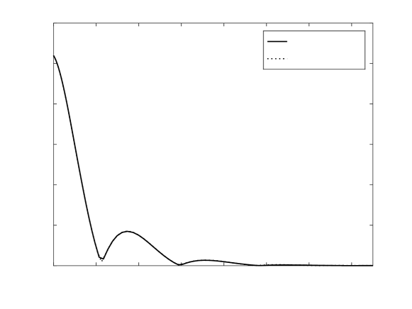
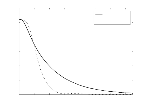
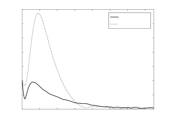
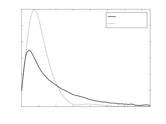
Figure 1: Simulation of observer in presence of noise: observer I: constant gain observer, observer II: variable gain observer
Theorem 2.

With Q𝑄Q and V𝑉V defined as constant symmetric positive definite matrices in the CRE equation (10), the observer system (11) converges to the system (1) exponentially fast under Assumption 1 for all (R¯​(0),b¯Ω​(0),p¯​(0),v¯​(0),bΒ―a​(0))βˆˆβ„3Γ—3×ℝ3×ℝ3×ℝ3×ℝ3¯𝑅0subscript¯𝑏Ω0¯𝑝0¯𝑣0subscriptΒ―π‘π‘Ž0superscriptℝ33superscriptℝ3superscriptℝ3superscriptℝ3superscriptℝ3(\bar{R}(0),\bar{b}_{\Omega}(0),\bar{p}(0),\bar{v}(0),\bar{b}_{a}(0))\in\mathbb{R}^{3\times 3}\times\mathbb{R}^{3}\times\mathbb{R}^{3}\times\mathbb{R}^{3}\times\mathbb{R}^{3}.

Proof.

Differentiating the errors, the error system is

EΛ™Rsubscript˙𝐸𝑅\displaystyle\dot{E}_{R} =βˆ’R​eΞ©Γ—βˆ’k1​ER,absent𝑅subscript𝑒subscriptΞ©subscriptπ‘˜1subscript𝐸𝑅\displaystyle=-Re_{\Omega_{\times}}-k_{1}E_{R}, (13a)
eΛ™Ξ©subscript˙𝑒Ω\displaystyle\dot{e}_{\Omega} =k2​π𝔰​𝔬​(3)​(RT​ER)∨,absentsubscriptπ‘˜2subscriptπœ‹π”°π”¬3subscriptsuperscript𝑅𝑇subscript𝐸𝑅\displaystyle=k_{2}\mathbb{\pi}_{\mathfrak{so}(3)}(R^{T}E_{R})_{\vee}, (13b)
eΛ™psubscript˙𝑒𝑝\displaystyle\dot{e}_{p} =evβˆ’K3​ep,absentsubscript𝑒𝑣subscript𝐾3subscript𝑒𝑝\displaystyle=e_{v}-K_{3}e_{p}, (13c)
eΛ™vsubscript˙𝑒𝑣\displaystyle\dot{e}_{v} =βˆ’R​eaβˆ’K4​ep,absent𝑅subscriptπ‘’π‘Žsubscript𝐾4subscript𝑒𝑝\displaystyle=-Re_{a}-K_{4}e_{p}, (13d)
eΛ™asubscriptΛ™π‘’π‘Ž\displaystyle\dot{e}_{a} =βˆ’K5​ep.absentsubscript𝐾5subscript𝑒𝑝\displaystyle=-K_{5}e_{p}. (13e)

Define x=(ep,ev,ea)π‘₯subscript𝑒𝑝subscript𝑒𝑣subscriptπ‘’π‘Žx=(e_{p},e_{v},e_{a}). Then the update equation for xπ‘₯x can be written as

xΛ™=A​(t)​xβˆ’P​(t)​CT​Q​C​x,Λ™π‘₯𝐴𝑑π‘₯𝑃𝑑superscript𝐢𝑇𝑄𝐢π‘₯\displaystyle\dot{x}=A(t)x-P(t)C^{T}QCx,

with A​(t)𝐴𝑑A(t) and C𝐢C as defined in equation (12).

Since the dynamics of R𝑅R-ΩΩ\Omega system are independent of the xπ‘₯x system, consider the two Lyapunov functions

V1subscript𝑉1\displaystyle V_{1} =k22β€‹βŸ¨ER,ER⟩+⟨eΞ©,eΩ⟩,absentsubscriptπ‘˜22subscript𝐸𝑅subscript𝐸𝑅subscript𝑒Ωsubscript𝑒Ω\displaystyle=\frac{k_{2}}{2}\langle E_{R},E_{R}\rangle+\langle e_{\Omega},e_{\Omega}\rangle,
V2subscript𝑉2\displaystyle V_{2} =xT​Pβˆ’1​x.absentsuperscriptπ‘₯𝑇superscript𝑃1π‘₯\displaystyle=x^{T}P^{-1}x.

The exponential convergence of the ERsubscript𝐸𝑅E_{R}-eΞ©subscript𝑒Ωe_{\Omega} system follows similar to that of Theorem 1.

Note that P​(t)𝑃𝑑P(t) is bounded above by qM​I9subscriptπ‘žπ‘€subscript𝐼9q_{M}I_{9} and below by qm​I9subscriptπ‘žπ‘šsubscript𝐼9q_{m}I_{9}. Defining

W1​(x)subscriptπ‘Š1π‘₯\displaystyle W_{1}(x) =β€–xβ€–2/qM,absentsuperscriptnormπ‘₯2subscriptπ‘žπ‘€\displaystyle=\|x\|^{2}/q_{M}, (14)
W2​(x)subscriptπ‘Š2π‘₯\displaystyle W_{2}(x) =β€–xβ€–2/qm,absentsuperscriptnormπ‘₯2subscriptπ‘žπ‘š\displaystyle=\|x\|^{2}/q_{m}, (15)

we have that W1​(x)≀V2​(t,x)≀W2​(x)subscriptπ‘Š1π‘₯subscript𝑉2𝑑π‘₯subscriptπ‘Š2π‘₯W_{1}(x)\leq V_{2}(t,x)\leq W_{2}(x). Differentiating V2subscript𝑉2V_{2} along the trajectory of the system (13),

VΛ™2subscript˙𝑉2\displaystyle\dot{V}_{2} =xT​((Aβˆ’P​CT​Q​C)T​Pβˆ’1+Pβˆ’1​(Aβˆ’P​CT​Q​C)βˆ’Pβˆ’1​P˙​Pβˆ’1)​xabsentsuperscriptπ‘₯𝑇superscript𝐴𝑃superscript𝐢𝑇𝑄𝐢𝑇superscript𝑃1superscript𝑃1𝐴𝑃superscript𝐢𝑇𝑄𝐢superscript𝑃1˙𝑃superscript𝑃1π‘₯\displaystyle=x^{T}((A-PC^{T}QC)^{T}P^{-1}+P^{-1}(A-PC^{T}QC)-P^{-1}\dot{P}P^{-1})x
=xT​(AT​Pβˆ’1+Pβˆ’1​Aβˆ’2​CT​Q​Cβˆ’Pβˆ’1​(A​P+P​ATβˆ’P​CT​Q​C​P+V)​Pβˆ’1)​xabsentsuperscriptπ‘₯𝑇superscript𝐴𝑇superscript𝑃1superscript𝑃1𝐴2superscript𝐢𝑇𝑄𝐢superscript𝑃1𝐴𝑃𝑃superscript𝐴𝑇𝑃superscript𝐢𝑇𝑄𝐢𝑃𝑉superscript𝑃1π‘₯\displaystyle=x^{T}(A^{T}P^{-1}+P^{-1}A-2C^{T}QC-P^{-1}(AP+PA^{T}-PC^{T}QCP+V)P^{-1})x
=βˆ’xT​(CT​Q​C+Pβˆ’1​V​Pβˆ’1)​xabsentsuperscriptπ‘₯𝑇superscript𝐢𝑇𝑄𝐢superscript𝑃1𝑉superscript𝑃1π‘₯\displaystyle=-x^{T}(C^{T}QC+P^{-1}VP^{-1})x

Note that CT​Q​Cβ‰₯0superscript𝐢𝑇𝑄𝐢0C^{T}QC\geq 0 since Q>0𝑄0Q>0, and Pβˆ’1​V​Pβˆ’1>0superscript𝑃1𝑉superscript𝑃10P^{-1}VP^{-1}>0 since P,V>0𝑃𝑉0P,V>0. Defining

W3​(x)=Ξ»m​i​n​(V)​‖xβ€–2qM2,subscriptπ‘Š3π‘₯subscriptπœ†π‘šπ‘–π‘›π‘‰superscriptnormπ‘₯2superscriptsubscriptπ‘žπ‘€2\displaystyle W_{3}(x)=\frac{\lambda_{min}(V)\|x\|^{2}}{q_{M}^{2}},

we see that W3​(x)≀λm​i​n​(V)​‖P​(t)βˆ’1​xβ€–2subscriptπ‘Š3π‘₯subscriptπœ†π‘šπ‘–π‘›π‘‰superscriptnorm𝑃superscript𝑑1π‘₯2W_{3}(x)\leq\lambda_{min}(V)\|P(t)^{-1}x\|^{2} since 1/qM1subscriptπ‘žπ‘€1/q_{M} is the smallest singular value of Pβˆ’1superscript𝑃1P^{-1} due to symmetricity of P𝑃P. Hence, W3​(x)β‰€βˆ’VΛ™2​(t,x)subscriptπ‘Š3π‘₯subscript˙𝑉2𝑑π‘₯W_{3}(x)\leq-\dot{V}_{2}(t,x), i.e. VΛ™2​(t,x)β‰€βˆ’W3​(x)subscript˙𝑉2𝑑π‘₯subscriptπ‘Š3π‘₯\dot{V}_{2}(t,x)\leq-W_{3}(x). Since W1​(x)≀V2​(t,x)≀W2​(x)subscriptπ‘Š1π‘₯subscript𝑉2𝑑π‘₯subscriptπ‘Š2π‘₯W_{1}(x)\leq V_{2}(t,x)\leq W_{2}(x) from equations (14) and (15), the system is exponentially stable (Theorem 4.10 [11]). Hence, the proposed variable gain observer is globally exponentially convergent.

∎
Refer to caption010203040-0.8-0.6-0.4-0.200.20.40.60.8Time(s)

bΞ©isubscript𝑏subscriptΩ𝑖b_{\Omega_{i}}

(a)
Refer to caption010203040-10-5051015Time(s)

baisubscript𝑏subscriptπ‘Žπ‘–b_{a_{i}}

(b)
Refer to caption010203040024681012Time(s)

bΞ©isubscript𝑏subscriptΩ𝑖b_{\Omega_{i}}

(c)
Refer to caption010203040-50510152025Time(s)

baisubscript𝑏subscriptπ‘Žπ‘–b_{a_{i}}

(d)
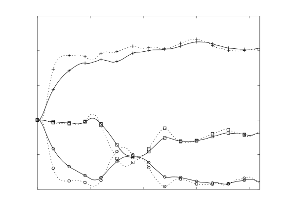
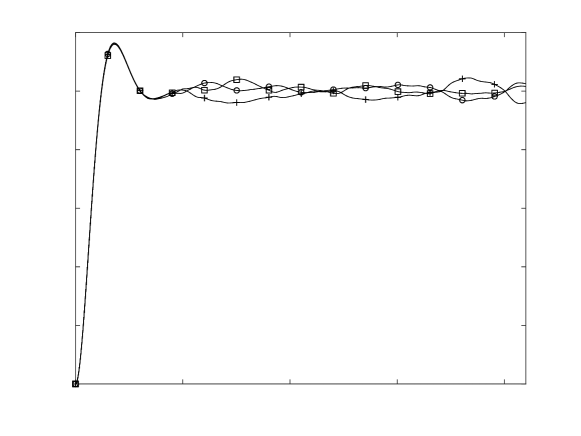
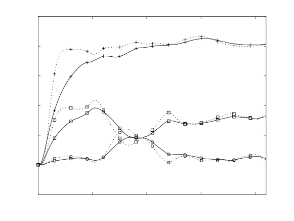
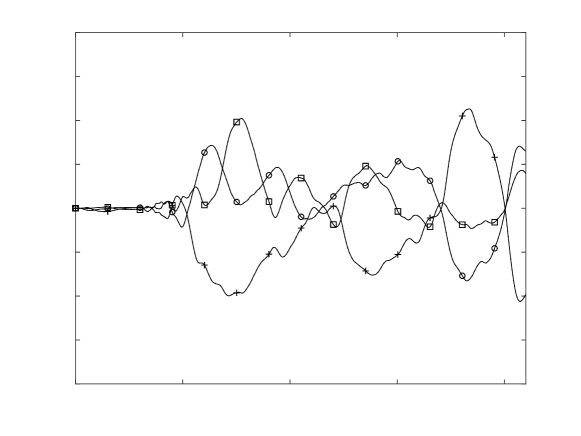
Figure 2: Experimental simulation of observer with data collected from a Intel Realsense T265: observer I: constant gain observer (solid line), observer II: variable gain observer (dashed line). Legend: square: b(Ξ©,a)xsubscript𝑏subscriptΞ©π‘Žπ‘₯b_{(\Omega,a)_{x}}, plus: b(Ξ©,a)ysubscript𝑏subscriptΞ©π‘Žπ‘¦b_{(\Omega,a)_{y}}, circle: b(Ξ©,a)zsubscript𝑏subscriptΞ©π‘Žπ‘§b_{(\Omega,a)_{z}}. Figures (a) and (b) correspond to no added bias, Figures (c) and (d) correspond to added bias of 10 units.

4 Numerical simulation

To simulate the observers, the system is initialised as (R​(0),p​(0),v​(0))=(exp⁑(βˆ’Ο€β€‹e3Γ—/3),03,03)𝑅0𝑝0𝑣0πœ‹subscript𝑒subscript33subscript03subscript03(R(0),p(0),v(0))=(\exp(-\pi e_{3_{\times}}/3),0_{3},0_{3}). The true angular velocity and linear acceleration of the system are chosen as (βˆ’sin⁑(10​t),cos⁑(10​t),0.6​sin⁑(5​t))10𝑑10𝑑0.65𝑑(-\sin(10t),\cos(10t),0.6\sin(5t)) and (cos⁑(0.5​t),sin⁑(0.5​t),cos⁑(t))0.5𝑑0.5𝑑𝑑(\cos(0.5t),\sin(0.5t),\cos(t)), respectively. The measurement of these values are corrupted with Gaussian noise of amplitude 0.010.010.01 and constant biases bΞ©=(βˆ’1,1,5)subscript𝑏Ω115b_{\Omega}=(-1,1,5) and ba=(1,βˆ’5,1)subscriptπ‘π‘Ž151b_{a}=(1,-5,1), respectively. For the measurement of the pose, we assume availability of l𝑙l markers (expressed as homogeneous vectors) b=[b1,b2,…,bl]βˆˆβ„4Γ—l𝑏subscript𝑏1subscript𝑏2…subscript𝑏𝑙superscriptℝ4𝑙b=[b_{1},b_{2},\ldots,b_{l}]\in\mathbb{R}^{4\times l} in the inertial frame and their corresponding measurements in the body frame r=[r1,r2,…,rl]βˆˆβ„4Γ—lπ‘Ÿsubscriptπ‘Ÿ1subscriptπ‘Ÿ2…subscriptπ‘Ÿπ‘™superscriptℝ4𝑙r=[r_{1},r_{2},\ldots,r_{l}]\in\mathbb{R}^{4\times l}, which are corrupted by Gaussian noise of amplitude 0.010.010.01. The measurement of the state of the system is arrived at using the landmark measurements as

[Rmpm01]=Ο€SE​(3)​(r​b†),matrixsubscriptπ‘…π‘šsubscriptπ‘π‘š01subscriptπœ‹SE3π‘Ÿsuperscript𝑏†\displaystyle\begin{bmatrix}R_{m}&p_{m}\\ 0&1\end{bmatrix}=\pi_{\textrm{SE}(3)}(rb^{\dagger}),

where Ο€SE​(3)​(A)subscriptπœ‹SE3𝐴\pi_{\textrm{SE}(3)}(A) represents projection of Aβˆˆβ„4Γ—4𝐴superscriptℝ44A\in\mathbb{R}^{4\times 4} onto the special Euclidean group of three dimensions, and b†superscript𝑏†b^{\dagger} represents the pseudo-inverse of b𝑏b.

The observer state (R¯​(0),p¯​(0),v¯​(0),b¯Ω​(0),bΒ―a​(0))=(I3,03,03,03,03)¯𝑅0¯𝑝0¯𝑣0subscript¯𝑏Ω0subscriptΒ―π‘π‘Ž0subscript𝐼3subscript03subscript03subscript03subscript03(\bar{R}(0),\bar{p}(0),\bar{v}(0),\bar{b}_{\Omega}(0),\bar{b}_{a}(0))=(I_{3},0_{3},0_{3},0_{3},0_{3}) is chosen as the initial state of both the observers. The simulation is run for 15 seconds. We choose k1=1,k2=1,k3=3.4,k4=5.5formulae-sequencesubscriptπ‘˜11formulae-sequencesubscriptπ‘˜21formulae-sequencesubscriptπ‘˜33.4subscriptπ‘˜45.5k_{1}=1,k_{2}=1,k_{3}=3.4,k_{4}=5.5 and k5=1.3subscriptπ‘˜51.3k_{5}=1.3 for the constant gain observer and k1=1,k2=1,P​(0)=I9,V=0.1​I9formulae-sequencesubscriptπ‘˜11formulae-sequencesubscriptπ‘˜21formulae-sequence𝑃0subscript𝐼9𝑉0.1subscript𝐼9k_{1}=1,k_{2}=1,P(0)=I_{9},V=0.1I_{9} and Q=I3𝑄subscript𝐼3Q=I_{3} for the variable gain observer. The results of the simulation is shown in Figure 1. From the simulation, it can be seen that the observers converge to the system state fairly quickly. Moreover, the bias value is estimated correctly even in the presence of noise in the system.

Table 1: Estimated Biases on data collected using Intel Realsense T265. Observer I: constant gain observer, observer II: variable gain observer
Observer I Observer II
bΞ©subscript𝑏Ωb_{\Omega} basubscriptπ‘π‘Žb_{a} bΞ©subscript𝑏Ωb_{\Omega} basubscriptπ‘π‘Žb_{a}
No added bias (0.05, -0.08, 0.03) (-2.28, 9.58, -7.69) (0.05, -0.08, 0.03) (-2.29, 9.72, -7.76)
Added bias of 10 units (9.90, 9.79, 9.88) (7.26, 19.11, 1.85) (9.9, 9.79, 9.88) (7.29, 19.3, 1.82)

5 Experiments

We perform experimental simulations to check the feasibility of the observer to estimate the bias in the angular velocity and the linear acceleration. We collect data of the pose using an Intel Realsense sensor. We use an IMU for the measurement of the angular velocity of the system, and an accelerometer for the measurement of the linear acceleration. We use the proposed observers for the estimation of the bias in the measurements. Since the noise in the measurement devices may be comparable to the bias, we also run the observers with the same data by adding a large(as compared to the noise) constant bias. In this experiment, we add (10,10,10)101010(10,10,10) to the measurements of the linear acceleration and angular velocity. The convergence of the bias to a constant value ensures that the bias has been accurately estimated.

The gains are chosen as k1=1,k2=1,k3=3.4,k4=5.5formulae-sequencesubscriptπ‘˜11formulae-sequencesubscriptπ‘˜21formulae-sequencesubscriptπ‘˜33.4subscriptπ‘˜45.5k_{1}=1,k_{2}=1,k_{3}=3.4,k_{4}=5.5 and k5=1.3subscriptπ‘˜51.3k_{5}=1.3 for the constant gain observer and as k1=1,k2=1,P​(0)=I9,V=0.1​I9formulae-sequencesubscriptπ‘˜11formulae-sequencesubscriptπ‘˜21formulae-sequence𝑃0subscript𝐼9𝑉0.1subscript𝐼9k_{1}=1,k_{2}=1,P(0)=I_{9},V=0.1I_{9}, and Q=I3𝑄subscript𝐼3Q=I_{3} for the variable gain observer. The simulation results can be seen in Figure 2. As expected, the biases converge to a constant value. The estimated biases are shown in Table 1. We see that the observer estimates the estimated biases well and converges to an almost constant value fairly quickly. We also see that the two experiments arrive at a similar value of bias (after removing the added bias of 10 units), and hence are consistent. The final estimate in the bias(taken as mean of the four biases arrived at) in the angular velocity is (βˆ’0.025,βˆ’0.145,βˆ’0.045)0.0250.1450.045(-0.025,-0.145,-0.045) and in the linear acceleration is (βˆ’2.505,9.428,βˆ’7.945)2.5059.4287.945(-2.505,9.428,-7.945).

6 Conclusion

We have designed two observers which show globally exponentially stable convergence to the rigid body rotation and translation system under assumptions of boundedness of angular velocity. These observers estimate the unknown bias in the linear acceleration and angular velocity measurements exponentially fast. The first observer assumes knowledge of bounds of the angular velocity, and proposes a constant gain observer. The second observer assumes no such knowledge, but provides a Riccati like observer, which is computationally expensive as compared to the first one. A possible future research topic would be proposing a constant gain observer without the knowledge of the bounds of angular velocity. An observer for discrete measurements with a continuous time system can also be designed by using the results of the proposed observer. Also, another possible future research topic would be using the ambient space extension technique to propose a machine learning based observer for the rigid body system.

References

  • [1] Axel Barrau and SilvΓ¨re Bonnabel. The invariant extended Kalman filter as a stable observer. IEEE Transactions on Automatic Control, 62(4):1797–1812, April 2017.
  • [2] Omar IbrahimΒ Dallal Bashi, Wan ZuhaΒ Wan Hasan, Norhafiz Azis, Suhaidi Shafie, and Hiroaki Wagatsuma. Unmanned aerial vehicle quadcopter: A review. Journal of Computational and Theoretical Nanoscience, 14(12):5663–5675, December 2017.
  • [3] Pedro Batista, Carlos Silvestre, and Paulo Oliveira. On the observability of linear motion quantities in navigation systems. Systems & Control Letters, 60(2):101–110, February 2011.
  • [4] SanjayΒ P. Bhat and DennisΒ S. Bernstein. A topological obstruction to global asymptotic stabilization of rotational motion and the unwinding phenomenon. In Proceedings of the 1998 American Control Conference. ACC (IEEE Cat. No.98CH36207), volumeΒ 5, pages 2785–2789, Philadelphia, PA, USA, June 1998. IEEE.
  • [5] SΓ©rgio BrΓ‘s, Maziar Izadi, Carlos Silvestre, Amit Sanyal, and Paulo Oliveira. Nonlinear observer for 3D rigid body motion estimation using Doppler measurements. IEEE Transactions on Automatic Control, 61(11):3580–3585, November 2016.
  • [6] DongΒ Eui Chang. Globally exponentially convergent continuous observers for velocity bias and state for invariant kinematic systems on matrix Lie groups. IEEE Transactions on Automatic Control, 66(7):3363–3369, July 2021.
  • [7] Simone de Marco, Minh-Duc Hua, Tarek Hamel, and Claude Samson. Position, velocity, attitude and accelerometer-bias estimation from IMU and bearing measurements. In 2020 European Control Conference (ECC), pages 1003–1008, Saint Petersburg, Russia, May 2020. IEEE.
  • [8] JayΒ A. Farrell. Aided Navigation: GPS with High Rate Sensors. McGraw Hill Professional, April 2008.
  • [9] HashimΒ A. Hashim. GPS-denied navigation: Attitude, position, linear velocity, and gravity estimation with nonlinear stochastic observer. In 2021 American Control Conference (ACC), pages 1149–1154, May 2021.
  • [10] Minh-Duc Hua and Guillaume Allibert. Riccati observer design for pose, linear velocity and gravity direction estimation using landmark position and IMU measurements. In 2018 IEEE Conference on Control Technology and Applications (CCTA), pages 1313–1318, August 2018.
  • [11] Hassan Khalil. Nonlinear Systems. Prentice Hall, Upper Saddle River, New Jersey, 2002.
  • [12] JaeΒ Hyeon Park, KarmvirΒ Singh Phogat, Whimin Kim, and DongΒ Eui Chang. Transversely stable extended Kalman filters for systems on manifolds in Euclidean spaces. Journal of Dynamic Systems, Measurement, and Control, 143(6), February 2021.
  • [13] Soham Shanbhag and DongΒ Eui Chang. Globally exponentially convergent observer for the rigid body system on SE(3). In 2022 IEEE 61st Conference on Decision and Control (CDC), pages 1257–1262, December 2022.
  • [14] José Fernandes Vasconcelos, Rita Cunha, Carlos Silvestre, and Paulo Oliveira. Landmark based nonlinear observer for rigid body attitude and position estimation. In 2007 46th IEEE Conference on Decision and Control, pages 1033–1038, December 2007.
  • [15] José Fernandes Vasconcelos, Rita Cunha, Carlos Silvestre, and Paulo Oliveira. A nonlinear position and attitude observer on SE(3) using landmark measurements. Systems & Control Letters, 59(3):155–166, March 2010.
  • [16] Miaomiao Wang and Abdelhamid Tayebi. Hybrid nonlinear observers for inertial navigation using landmark measurements. IEEE Transactions on Automatic Control, 65(12):5173–5188, December 2020.