Probing orbits of stellar mass objects deep in galactic nuclei with quasi-periodic eruptions
Abstract
Quasi-periodic eruptions (QPEs) are intense repeating soft X-ray bursts with recurrence times about a few to ten hours from nearby galactic nuclei. The origin of QPEs is still unclear. In this work, we investigated the extreme mass ratio inspiral (EMRI) + accretion disk model, where the disk is formed from a previous tidal disruption event (TDE). In this EMRI+TDE disk model, the QPEs are the result of collisions between a TDE disk and a stellar mass object (a stellar mass black hole or a main sequence star) orbiting around a supermassive black hole (SMBH) in galactic nuclei. This model is flexible and comprehensive in recovering different aspects of QPE observations. If this interpretation is correct, QPEs will be invaluable in probing the orbits of stellar mass objects in the vicinity of SMBHs, and further inferring the formation of EMRIs which is one the primary targets of spaceborne gravitational wave missions. Taking GSN 069 as an example, we find the EMRI wherein is of low eccentricity ( at 3- confidence level) and semi-major axis about gravitational radii of the central SMBH, which is consistent with the prediction of the wet EMRI formation channel, while incompatible with alternatives.
I Introduction
In the past decade, X-ray quasi-periodic eruptions (QPEs) have been detected in nearby galactic nuclei Sun et al. (2013); Giustini et al. (2020); Arcodia et al. (2021, 2022); Chakraborty et al. (2021) which host low-mass ( at most) central supermassive black holes (SMBHs) Wevers et al. (2022); Miniutti et al. (2023a). QPEs are fast bright soft X-ray bursts repeating every few hours with peak X-ray luminosity ergs s-1. QPEs have thermal-like X-ray spectra with temperatures eV, in contrast with the temperatures eV in the quiescent state. The presence of a narrow line region in all QPE host galaxies implies that a long-lived active galactic nucleus (AGN) likely plays an integral role in the QPEs, while the absence of luminous broad emission lines indicates that none of the central SMBHs are currently actively accreting, i.e., they are all likely recently switched-off AGNs Wevers et al. (2022). In addition, QPEs similar to tidal disruption events (TDEs) are preferentially found in post-starburst galaxies Wevers et al. (2022), and two QPE sources (GSN 069 and XMMSL1 J024916.6-04124) and a candidate (AT 2019vcb), have been directly associated with X-ray TDEs Shu et al. (2018); Sheng et al. (2021); Chakraborty et al. (2021); Miniutti et al. (2023a); Quintin et al. (2023). A recent XMM-Newton observation of GSN 069 identified the reappearance of QPEs after two years of absence Miniutti et al. (2023a). This observation result shows that QPEs may only be present below a quiescent luminosity threshold , where is the Eddington luminosity, and a new phase shows up in the QPE reappearance where the intensity and the temperature of two QPEs become different. Long term observation of yields more interesting features of GSN 069 Miniutti et al. (2023b), e.g., the quasi-periodic oscillations (QPOs) in the quiescent state following the QPEs, long-term evolution of the quiescent level emission is consistent with a TDE or even possibly a repeating TDE, and QPEs measured in higher energy bands are stronger, peak earlier, and have shorter duration than when measured at lower energies.
Many models have been proposed for explaining the physical origin of QPEs, based on different disk instabilities111The classical limit-cycle instability in AGN disks is disfavored because the the QPE periods, burst timescales and burst profiles cannot be reconciled with the limit-cycle prediction Arcodia et al. (2021); Liu (2021). Raj and Nixon (2021); Pan et al. (2022a, 2023); Kaur et al. (2023); Śniegowska et al. (2023), self-lensing binary massive black hole Ingram et al. (2021), mass transfer at pericenter from stars or white dwarfs orbiting around the SMBH King (2020, 2022, 2023); Chen et al. (2022); Wang et al. (2022); Zhao et al. (2022); Metzger et al. (2022); Lu and Quataert (2022); Krolik and Linial (2022); Linial and Sari (2023), (periodic) impacts between a stellar-mass object (SMO), a star or a stellar mass black hole (sBH), and the accretion disk that is formed following a recent TDE (dubbed as EMRI+TDE disk model) Suková et al. (2021); Xian et al. (2021); Tagawa and Haiman (2023); Linial and Metzger (2023a); Franchini et al. (2023). These models can explain some of the features in the QPE light curves (mainly GSN 069), there is no model producing diverse features of different QPE sources (see more discussions in e.g. Miniutti et al. (2019); Giustini et al. (2020); Arcodia et al. (2021, 2022); Chakraborty et al. (2021); Wevers et al. (2022); Miniutti et al. (2023a, b)).
Recently, Linial et al. Linial and Metzger (2023a) and Franchini et al. Franchini et al. (2023) pointed out the EMRI + TDE disk model is flexible in recovering comprehensive features of different QPEs. In this EMRI+TDE disk model, the stellar mass object (SMO) could be a sBH or a main sequence star, and the two share many similar model predictions, e.g., the long-short pattern in the QPE recurrence times and the strong-weak pattern in the QPE intensities (see Franchini et al. (2023); Linial and Metzger (2023a, b) for details), therefore it seems hard to distinguish the two with the existing QPE observations. In the majority of this work, we tend not to distinguish them and we will briefly discuss their different predictions that might be tested by near future observations in the final part of this paper. We first refine the flare model following the analytic supernova explosion model developed by Arnett Arnett (1980), and have been used in modelling the optical flares of OJ 287 Lehto and Valtonen (1996); Pihajoki (2016) and SDSSJ1430+2303 Jiang et al. (2022). With this refinement, we find the model fitting to the QPE light curves with reasonable precision though the the effective temperatures at the light curve peaks in the best-fit model is in tension with the observation values. Due to this limitation of the plasma ball emission model, we consider an alternative phenomenological model where the light curve consists of a rising part and a decay part with different timescales. We apply both models to the QPEs from GSN 069 and find out the starting time of each flare, with which we constrain the EMRI orbital parameters. We find the EMRI orbit inferred from these QPEs is of low eccentricity ( at 3- confidence level) and semi-major axis , where is the gravitational radius of the central SMBH. If the EMRI+TDE disk is indeed the origin of QPEs, the EMRI orbital parameters inferred from the QPEs will be invaluable in probing the EMRI formation channels. As for the GSN 069 EMRI, we find it is highly unlikely comes from the loss-cone channel or the Hills mechanism, while is consistent with the wet channel expectation.
This paper is organized as follows. In Section II , we briefly review the flare emission mechanism, introduce two analytic model for fitting the QPE light curves, and the EMRI equations of motion (EoM). In Section III , we fit the QPE light curves finding out the starting time of each flare, with which we constrain the EMRI orbital parameters. In Section IV, we summarize this paper by evaluating the performance of the EMRI+disk model predictions, discussing the implications of QPEs on EMRI formation channels and possible observable signatures for distinguishing stellar EMRIs versus sBH EMRIs. In Appendix A, we include the detailed corner plots of emission model parameters and the flare timing model parameters. In Appendix B, we analyze the orbital stability of the SMO after a possible close-by scattering with a TDE remnant star. In Appendix C, we show some hydrodynamic (HD) simulation results of SMO-disk collisions and infer possible observational features in the resulted light curves. In this paper, we use geometrical units with if not specified otherwise.
II QPE model: EMRI+TDE disk
Fig. 1 displays the GSN 069 QPEs found in 5 XMM Newton observations. The peak luminosity, recurrence time, and duration of QPEs are ergs/s, hours and hour, respectively. In this section, we will first sketch the EMRI+TDE disk model identifying the parameter space that is consistent with above energy budget and time scales, then explain the details of the emission models for fitting each individual QPE light curve and the EMRI model for fitting the starting times of all QPEs.
II.1 Emission model
As a the SMO orbiting around the SMBH and cross the accretion disk, the relative velocity between the SMO and the local accretion flow in general is higher than the local sound speed , and the gas in the disk will be compressed and heated by the shock wave. For sBHs, the accretion radius is in general much larger than the geometrical size . As shown by simulations in Ref. Ivanov et al. (1998), the heated gas expands along the shocked tunnel and forms a hot, optically thick, radiation-dominated plasma ball on each side of the disk. The hot plasma ball cools down due to (nearly) adiabatic expansion and thermal radiation. For stars, the whole process is similar except now the geometrical radius plays the role of the accretion radius in the sBH case.
We consider the standard disk model Shakura and Sunyaev (1973), where the disk structure in the radiation dominated regime can be analytically expressed as Kocsis et al. (2011)
| (1) | ||||
where is the scale height of the disk from the mid-plane, is the disk surface density and we have defined with the Eddington accretion rate.
For a star, the energy loss after crossing a disk is simply
| (2) | ||||
where the factor in the first line takes both the thermal energy and the kinetic energy of the shocked gas into account, , is the mass of the shocked gas Linial and Metzger (2023a), and we have used the approximation with the local Keplerian velocity, where is the angle between the sBH orbital plane and the disk plane.
For a sBH moving in a uniform gas cloud, the gravitational drag from the perturbed gas is Chandrasekhar (1943); Rephaeli and Salpeter (1980); Binney and Tremaine (1987)
| (3) | ||||
where is the gas density; is the sBH mass; is the ratio of relative velocity over the gas particle velocity dispersion (approximated by the local sound speed ), and we have used the approximation in the second line; is the Coulomb logarithm with the maximum/minimum cutoff distance associated to the interaction. The cutoff distance is the maximum extent of the wake , while was identified either as the accretor size Shankar et al. (1993); Ruffert and Arnett (1994); Edgar (2004); Chapon et al. (2013) or as the stand off distance Thun et al. (2016). With these two different identifications, we have , where we have used the fiducial values and in the approximate equal sign. As a result, the sBH loses energy after crossing a disk 222In estimating the sBH energy loss in crossing the disk, people easily use the approximation . In fact, above is merely the amount of gas that is supposed to be accreted by the sBH, which is only a fraction of shocked gas (the shock size is larger than the accretion radius by quite a few times (see e.g. Hunt, 1971, 1979; Shima et al., 1985; Ruffert and Arnett, 1994; Ruffert, 1996)). The more accurate estimate of the sBH energy loss would be Eq. (4), which was derived in Ref. Rephaeli and Salpeter (1980) and had been verified with hydrodynamic simulations (see e.g. Shima et al., 1985; Shankar et al., 1993; Ruffert and Arnett, 1994; Ruffert, 1996; Chapon et al., 2013).
| (4) | ||||
where is the length of the sBH orbit inside the disk, and we have defined .
In order to find out the starting time of each flare, we consider the following two emission models: an expanding plasma ball emission model and a phenomenological model.
II.1.1 Plasma ball model
In general, the post-shock gas is not uniformly compressed, heated or accelerated depending on where it crosses the shock front (see e.g. Hunt, 1971, 1979; Shima et al., 1985; Ruffert and Arnett, 1994; Ruffert, 1996, for detailed simulations). For modelling the emission of the shocked gas, we simplify the shocked gas as a uniform plasma ball with initial size and initial surface temperature . Following Arnett Arnett (1980), We model the plasma ball expansion, cooling and radiation as follows.
Considering a spherical plasma ball expanding uniformly, the evolution of the expanding shell follows the first law of thermodynamics, which states, in the Lagrangian coordinates,
| (5) |
where , are the specific energy and volume, and are the pressure and the radiation luminosity, and is the total mass enclosed by the shell considered. In the diffusion approximation, is
| (6) |
where is the opacity dominated by Thomson scattering.
Adiabatic homologous expansion of a photon-dominated gas () gives and , where is the boundary of the plasma ball. With these two relations, we can now write
| (7) | ||||
| (8) | ||||
| (9) |
where is a dimensionless comoving radial coordinate. In the time scale of our consideration, the outer boundary of the plasma ball is expanding at a constant speed
| (10) |
is the expansion timescale and is the expanding velocity scale. In (7), we separate the space and time dependence of temperature.
Plugging (6) to (9) into (5) and separate the PDE, we have
| (11) | ||||
| (12) |
where is the eignvalue determined by the boundary condition, is the diffusion time scale. We consider the ’radiative zero’ boundary condition Arnett (1980) (). Together with the trivial boundary condition at the center , the solution of (11) is
| (13) |
the eigenvalue . The time evolution equation (12) can be solved with the trivial initial condition , whose solution is
| (14) |
With (10), (13) and (14), the temperature distribution and evolution is obtained. We now return to the surface luminosity. Plugging (7), (10), (13), (14) into (6) and take , we have
| (15) |
Afterwards, we choose the effective temperature as the parameter of our model, which can be directly obtained from the surface luminosity
| (16) |
Applying this model to QPEs, we find the soft X-ray (0.2-2keV) luminosity
| (17) |
where the effective temperature is determined by (16) and the plasma ball radius is determined by (10). The intrinsic parameters of our model are in addition to the flare staring time . For the purpose of model parameter inference, we find parameters are better constrained, which are chosen as the model intrinsic parameters hereafter.
II.1.2 Phenomenological model
In additional to the above expanding plasma ball emission model, we also consider the following alternative phenomenological light curve model Norris et al. (2005); Arcodia et al. (2022)
| (18) |
where . Following Ref. Norris et al. (2005), we define the flare starting time as when the flux is of the peak value, i.e., . Therefore only 3 out of the 4 time variables are independent, and we take and as the independent model parameters.
In addition to the QPEs, quasi-periodic oscillations (QPOs) has been identified in the quiescent state luminosity, we therefore model the background luminosity as
| (19) |
where is average background luminosity, are the QPO amplitude, period and initial phase, respectively.
II.2 Flare timing
In general, the sBH collides the accretion twice per orbit, and the propagation times of two flares produced by the collisions to the observer are different due to different propagation paths.
For convenience, we model the motion of the sBH as a geodesic in the Schwarzschild spacetime. Considering an orbit with semimajor axis and eccentricity , the pericenter and apocenter distance are the roots to the effective potential Chandrasekhar (1983)
| (20) |
where all the radii/distances are formulated in units of the graviational radius . From the effective potential, it is straightforward to obtain the orbital energy and angular momentum . The equations of motion (EoMs) in the Schwarzschild spacetime can be derived from the Hamiltonian
| (21) |
where is the Schwarzschild metric. Considering the simple case where the orbit lies on the equator, we obtain
| (22) | ||||
where and dots are the derivative w.r.t. to time and is the azimuth angle. Combining with initial condition (i.e., starting from the apocenter), we obtain the orbital motion .
Assuming the accretion disk lies on the equator plane (the disk angular momentum is in the direction, i.e. ), and the orbital plane lies on the plane, and the two coordinate frames are related by Euler rotations , where
| (23) |
and
| (24) |
The orbital motion in the two frames are
| (25) |
and
| (26) |
respectively. Specifically, is the angle between the disk plane and the orbital plane, i.e., .
Using a coordinate frame such that the line of sight (los) lies in the plane with . The observable collisions happen when , where the sign depend on the observation is on the upper/lower half plane. The propagation times of different flares at different collision locations to the observer will also be different. We can write , where
| (27) | ||||
are corrections caused by different path lengths and different Shapiro delays Shapiro (1964), respectively.
To summarize, there are parameters in the flare timing model: the intrinsic orbital parameters , the extrinsic orbital parameters , the los angle , the time at apocenter right before the 1st flare observed, and the mass of the SMBH or equivalently the Newtonian orbital period . Without loss of generality, we set , i.e., the observer locates in the upper half plane, and the observed flares start when the EMRI crosses the upper surface of the disk (we set the disk thickness as ).
III Applying the EMRI+TDE disk model to GSN 069 QPEs
For a given EMRI system and a TDE accretion disk, we can in principle predict the collision times between the SMO and the disk, the initial condition of plasma ball from each collision, and the resulting QPE light curve. Both the EMRI orbital parameters and the disk model parameters can be constrained simultaneously from the QPE light curves. In this work, we choose to constrain the EMRI kinematics and the plasma ball emission separately: we first fit each QPE with the flare model and obtain the starting time of each flare , which is identified as the observed disk crossing time. In this way, the EMRI kinematics is minimally plagued by the uncertainties in the disk model because the the disk crossing time inferred from the QPE light curve is not expected to be sensitive to the disk model.
According to the Bayes theorem, the posterior of parameters given data is
| (28) |
where is the likelihood of detecting data given a model with parameters and is the parameter prior assumed. For the emission model, the likelihood is defined as
| (29) |
where are the measured QPE luminosity and errorbar at , respectively, is the model predicted luminosity [Eqs. (17,19], and is a scale factor taking possible calibration uncertainty into account. Therefore we have model parameters for each flare in the expanding plasma ball model, and for each flare in the phenomenological model. The posterior of each flare is then fed into the flare timing model.
For the flare timing model, the likelihood is defined in a similar way as
| (30) |
where is the model predicted starting time of -th flare in the observer’s frame [Eq. (27)], and are the flare starting time and the uncertainty of -th flare (see Table 1). In the same way we have included a scale factor taking possible systematics/unmodeled physics processes into consideration. Therefore we have parameters in the flare timing model. The model parameter inferences are performed using the dynesty Speagle (2020) and nessai Williams (2021) algorithm in the package Bilby Ashton et al. (2019).
III.1 GSN 069 QPE light curves
GSN 069 is the first QPE source discovered, and has been monitored extensively in the past decade, including XMM 1-12 and Chandra Miniutti et al. (2023a, b). From the quiescent state light curves, it is likely that two (partial) TDEs has happened. QPEs are found only in XMM 3-6 and 12 and the Chandra observation, when the quiescent state luminosity is low.
We reprocessed the raw data from EPIC-pn camera Strüder et al. (2001) of the XMM-Newton mission, using the latest XMM–Newton Science Analysis System (SAS) and the Current Calibration Files (CCF). The photon arrival times are all barycentre-corrected in the DE405-ICRS reference system. The count-rate-luminosity conversion is accomplished with XSPEC Arnaud (1996). The result light curves are shown in Fig. 1.333We did not include the Chandra observation at 14 Feb 2019 in our analysis, because the data quality is much lower compared with that in XMM-Newton observations, especially the discontinuous features in the count rates around the background level make it hard to pin down the flare starting times. This is attributed to the much smaller effective area of Chandra.
During XMM 3-5 and Chandra (regular phase), the quiescent state luminosity is slowly declining and the QPEs show clear long-short pattern in the occurrence times and strong-weak pattern in the intensities. During XMM 6, the quiescent state luminosity is climbing up probably in the rising phase of the second TDE and the QPEs become irregular in the sense that the alternating strong-weak pattern is not well preserved, where the first flare does not fit in either the strong or the weak ones, though flares 2-4 still follow the alternating long-short and strong-weak patterns (see Fig. 1). During the recent observation epoch XMM 12, only two QPEs were detected limited by the short exposure time and it is unclear whether the QPEs have settled down to a new regular phase or not.
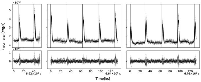
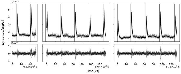
From Fig. 1, it is evident that there is an alternating long-short pattern in the QPE recurrence times with ks, and is approximately a constant. To quantify these features, we fit these QPEs with the two flare models. In Fig. 2, we show the 0.2-2 keV light curves of GSN 069 QPEs from XMM 3-5 along with the best-fit emission model (see the corner plot of the model parameter posterior in Fig. 7). From the residue plots in the lower panels, we see that the fits are reasonable for the majority parts of the light curves except around the peaks where the sharp turnovers are not captured by the fits, and around the flare staring times where the precursor like features prior to the main flares cannot be captured either. These limitations also motivate us to consider the alternative phenomenological light curve model (18). In Fig. 3, we show the results of the best-fit phenomenological model, which largely improves the residues around the light curve peaks and yield consistent flare starting times with those from the plasma ball model. The standing-out residues around the flare starting times imply possible processes that are not modeled in either model (see more discussion in Appendix C where we conduct hydrodynamic simulations of SMO-disk collisions trying to identifying the unmodeled processes by comparing the simulations with the light curves).
| Plasma ball model | |||||
| XMM3 flare 1 | |||||
| 2 | |||||
| XMM4 flare 1 | |||||
| 2 | |||||
| 3 | |||||
| 4 | |||||
| 5 | |||||
| XMM5 flare 1 | |||||
| 2 | |||||
| 3 | |||||
| 4 | |||||
| 5 | |||||
| XMM6 flare 1 | |||||
| 2 | |||||
| 3 | |||||
| 4 | |||||
| XMM12 flare 1 | |||||
| 2 |
| Phenomen model | |||||
| XMM3 flare 1 | |||||
| 2 | |||||
| XMM4 flare 1 | |||||
| 2 | |||||
| 3 | |||||
| 4 | |||||
| 5 | |||||
| XMM5 flare 1 | |||||
| 2 | |||||
| 3 | |||||
| 4 | |||||
| 5 | |||||
| XMM6 flare 1 | |||||
| 2 | |||||
| 3 | |||||
| 4 | |||||
| XMM12 flare 1 | |||||
| 2 |
In Table 1 and Table 2, we list all the flare starting times , the QPO periods and the intervals fitted from the QPE light curves with the plasma ball model and the phenomenological model respectively. With the flare starting times , we are to quantify the long-short pattern in the QPE recurrence times. In XMM 3, 2 flares are observed, therefore only the short time can be calculated. In XMM 4, 5 flares are observed, and we define
| (31) | ||||
and the definitions are similar in XMM 5. In XMM 6, 4 flares are observed with the 1st being an outlier, and we define
| (32) | ||||
The measured time intervals and are consistent with each assuming two different light curve models. To quantify the evolution of period , we fit the with a linear relation and we find the slope/the change rate is consistent with zero as
| (33) |
at - confidence level.
III.2 EMRI orbital parameters
As explained in the previous subsection, QPEs found in XMM 3-5 are in the regular phase and we will focus on the QPE timing in these 3 observations for our EMRI orbit analysis (see Summary section for more discussions about observations XMM 6 and 12).
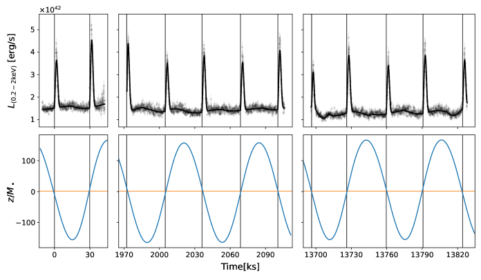
In Fig. 4, we show the EMRI orbit of the best-fit flare timing model (with orbital parameters , and the corresponding SMBH mass ), along with the starting time of each flare (Table 1). In this model, is simply the orbital period which is a constant if the TDE disk lies on the equator and stays in a steady state as assumed, while the alternating recurrence times are the result of a non-circular orbit plus the different photon propagation times to the observer, and the variation of is the result of the SMO orbital precession.
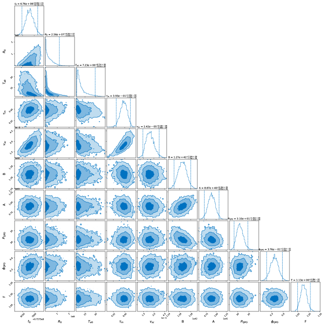
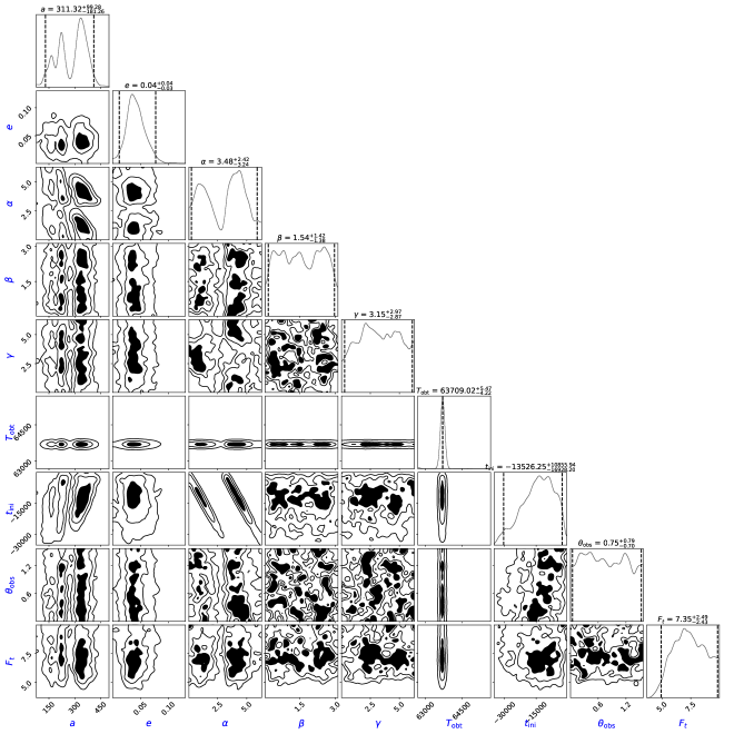
The posterior corner plot of all the model parameters is shown in Fig. 9 in Appendix A, where the orbital parameters are constrained as
| (34) | ||||
at 2- confidence level, respectively. The constraint of the SMBH mass is therefore at 2- confidence level. In fact, the flare timing contains more information of the SMBH mass than what the simple confidence level shows: there are 3 peaks in the posterior of the semi-major axis locating at , respectively, which corresponding to 3 favored values of the SMBH mass .
IV Summary and discussion
In this section, we first summarize different aspects of QPE observations in addition to the recurrence timescales ( a few hours) and the luminosity magnitudes of QPE flares in soft X-rays ( ergs/s), and evaluate the performance of the EMRI+TDE disk model in interpreting these observations. Based on the orbital parameters inferred from the flare timing, we then examine which formation channel the EMRI may come from. We conclude this section with a brief discussion about possible ways to distinguish the two and limitations of the flaring time model used in this paper.
IV.1 Observations versus model predictions
1. Alternating long-short occurrence times: in all the confirmed QPE sources to date with more than 3 flares detected (GSN 069, eRO-QPE1, eRO-QPE2, and RX J1301.9+2747), QPEs have two alternating occurrence times and Miniutti et al. (2019); Giustini et al. (2020); Arcodia et al. (2021, 2022). In the EMRI+TDE disk model, the secondary SMO crosses the accretion disk twice per orbit and two different occurrence times and alternate as a result of non-circular orbit and different delays of two consecutive collisions [see Eq. (27)]. (✓)
2. Alternating strong-weak QPE intensities: strong-weak QPEs alternately occur Miniutti et al. (2019); Giustini et al. (2020); Arcodia et al. (2021, 2022); Chakraborty et al. (2021). In the EMRI+TDE disk model, the secondary BH crosses the accretion disk twice per orbit producing two different flares because the two disk crossings are not identical to each other depending on the orbit eccentricity. (✓)
3. Spectral evolution: QPEs measured in higher energy bands are stronger, peak earlier, and have shorter duration than when measured at lower energies Miniutti et al. (2019); Giustini et al. (2020); Arcodia et al. (2021, 2022); Chakraborty et al. (2021); Miniutti et al. (2023b). The QPE spectral evolution perfectly matches the flare model prediction where the QPE emission comes from an expanding and cooling plasma ball. (✓)
4. Light curve profile: a common feature of QPEs is the fast rise and slow decay light curve profile with a low QPE duty cycle (a few percent) Miniutti et al. (2019); Giustini et al. (2020); Arcodia et al. (2021, 2022); Chakraborty et al. (2021). Similar to supernova explosions, the thermal radiation from a freely expanding and cooling plasma ball naturally produces the fast rise and slow decay light curve. (✓)
5. Association with TDEs: two QPE sources (GSN 069 and XMMSL1 J024916.6-04124) and a candidate (AT 2019vcb), have been directly associated with X-ray TDEs Shu et al. (2018); Sheng et al. (2021); Chakraborty et al. (2021); Miniutti et al. (2023a); Quintin et al. (2023). See the next point. (✓)
6. Association with past AGN activities, and not with on-going AGNs: the presence of narrow lines in all QPE host galaxies and the absence of luminous broad emission lines indicates that they are recently switched-off AGNs Wevers et al. (2022); Patra et al. (2023) (but see also Metzger et al. (2022) for a different interpretation). In on-going AGNs, the majority of SMOs in the vicinity of the SMBH are those captured onto the AGN accretion disk Pan et al. (2022b), as a result the number of SMOs crossing the AGN disk is suppressed, therefore no QPE association with on-going AGNs. In recently turned-off AGNs, SMOs are accumulated on the equator of the SMBH with (see Pan et al. (2022b); Pan and Yang (2021a) for full Fokker-Planck calculation or Section IV.2 for a sketch), while the accretion disk formed from a TDE is in general not exactly aligned with the equator, therefore QPEs are produced as the SMO crossing the TDE formed accretion disk. (✓)
7. (Anti-)association with SMBH mass: QPEs are preferentially found in nuclei of dwarf galaxies, where the SMBHs are relatively light with mass no more than a few times Wevers et al. (2022); Miniutti et al. (2023a). In the EMRI+TDE disk model, this anti-association with the SMBH mass comes from the finite size of the TDE formed accretion disk. Assuming an -disk of total mass , we have the disk size
| (35) |
For more massive SMBHs, the disk is smaller, and for a SMBH heavier than . The chance of SMOs with crossing the TDE formed disk around a more massive SMBH is lower. (✓)
8. (Anti-)association with SMBH accretion rate in quiescent state: long-term observation of GSN 069 shows that QPEs may only be present below a quiescent luminosity threshold Miniutti et al. (2023a). There are two possible origins of this anti-association: the ratio of the QPE luminosity to the disk luminosity in the same energy band depends on the disk accretion rate Franchini et al. (2023), or QPEs are delayed relative to the TDE by a time interval (which is about a few years in the case of GSN 069).
In the disk model, the disk surface density and the energy deposited in the SMO-disk collision [Eqs. (2,4)] is therefore lower for the higher accretion rate case. The thermal luminosity from the accretion disk is higher in the higher accretion case and the dependence is more sensitive for the soft X-ray luminosity . As a result, the QPE is harder to identify from the luminous background in the higher accretion rate case (see Franchini et al. (2023) for the explanation in terms of QPE temperatures and the disk temperature).
In general, the SMO orbital angular momentum direction is misaligned with the SMBH spin direction and the newly formed disk in a TDE is consequently misaligned. The misaligned disk initially precess like a rigid body before settling down to a non-precessing warped disk Liska et al. (2018); Chatterjee et al. (2020, 2023). In a recently turned-off AGN, the sBHs are preferentially found on the equator of the SMBH. As a result, the sBH is expected to be highly inclined with respect to the new TDE disk when the sBH-disk collisions are less energetic [Eq. (4)], and QPEs emerge only when the two become nearly aligned and the collisions are sufficiently energetic. This scenario works for sBH EMRIs only, where the emergence of QPEs is delayed by the disk alignment timescale, the accurate value of which is not accurately calculated Stone and Loeb (2012); Franchini et al. (2016). (✓)
9. Stability: during the observations XMM 3-5 (regular phase dubbed in Miniutti et al. (2023a)), the QPE occurrence times are stable with variation rate consistent with zero (see Eq. (33)). The sBH orbital period change rate due to disk crossing turns out to be (Eq. [4])
| (36) | ||||
where . The orbital change rate is consistent with the observed . The star orbital period change rate is given by Linial and Quataert (2023)
| (37) |
where . The orbital period change rate is also consistent with the current observation constraint. (✓)
10. Association with QPOs in quiescent state: in the old phase (XMM 3-5) quiescent level QPOs were detected with a period close to the corresponding QPE recurrence times (see Tables 1, 2), and a ks delay with respect to the QPEs Miniutti et al. (2023a, b). It is unclear whether the periodic EMRI impacts on the accretion disk are able to produce the quiescent level QPOs with correct time delay, period and amplitude. 444Previous simulations show that the accretion rate of the central BH is indeed modulated by periodic stellar-disk collisions Suková et al. (2021). (?)
11. New QPE phase in GSN 069: during the old phase (XMM 3-5), both the QPE intensities and occurrence times alternated with ks , ks and ks. During the irregular phase (XMM 6) which is on the rise of TDE 2, the QPE occurrence times observed do not follow the alternating patterns exactly with the 1st flare fitting in neither the strong ones nor the weak ones, though flares 2-4 still follow the alternating long-short and strong-weak patterns with ks , ks and ks. After disappeared for two years (XMM 7-11), QPEs reappeared (XMM 12) with quite different occurrence times from those in the old phase or the irregular phase: ks and is not fully resolved because only two QPEs have been detected Miniutti et al. (2023a). By fitting the variation in the quiescent level with a sine function, the period was constrained to be ks, however this period suspiciously coincides with the exposure time and the statistical quality of the fit is poor with reduced ( and ) Miniutti et al. (2023a, b). This QPO period has been speculated to be same to the QPE period in the new phase, , though this speculated relation is not observed in the previous phases where the QPO periods are found in the range of (see Tables 1 and 2). Further measurements with longer exposure time are needed to confirm whether a different QPE period emerges in the new phase.
In the EMRI+ TDE disk model, the shorter is a result of a puffier disk due to the higher accretion rate sourced by the TDE 2 and consequently a larger fraction
| (38) |
of the EMRI orbit is embedded in the disk. As a result, orbit stays above the disk which is visible to the observer making a shorter , and the remaining hides in or below the disk which is invisible. This geometrical effect of the disk thickness may also contributes to the shorter in XMM 6 which is on the rise of TDE 2. (✓)
To identify the true origin(s) of QPEs, all the existing models should be tested against these observations. Taking GSN 069 as an example, the alternating long-short recurrence pattern and a stable (see Fig. 1) together pose a huge challenge for the single-period models. In these models, there is no natural explanation to either of them without a twofold fine tuning: alternating delay-advance in the recurrence times for producing the alternating long-short pattern, and cancellation of consecutive delay/advance for producing a stable . In the EMRI+TDE disk model, the alternating long-short pattern and the constant are natural consequences of a non-circular orbit, and most of the QPE observations summarized above can be quantitatively recovered though it is unclear whether quiescent-state QPOs can be naturally generated.
IV.2 Implications of QPEs on EMRI formation
If QPEs are indeed sourced by impacts of SMOs and accretion disks formed from TDEs, the EMRI orbital parameters will be invaluable for inferring the EMRI formation channels. These SMOs may be captured by the SMBH via the (dry) loss-cone channel Hopman and Alexander (2005); Preto and Amaro-Seoane (2010); Bar-Or and Alexander (2016); Babak et al. (2017); Amaro-Seoane (2018); Broggi et al. (2022), Hills mechanism Miller et al. (2005); Raveh and Perets (2021) or the (wet) AGN disk channel Pan and Yang (2021b); Pan et al. (2021); Pan and Yang (2021a); Pan et al. (2022b); Derdzinski and Mayer (2023). The EMRI orbits inferred from the 6 QPE sources are of similar properties, with low eccentricity and with pericenter distance Franchini et al. (2023); Linial and Metzger (2023a). These orbital parameters are are roughly consistent with the (wet) EMRIs formed in AGN disks, where the wet EMRIs are expected to be nearly circular, and concentrate around at the end of an AGN phase Pan and Yang (2021b); Pan et al. (2021); Pan and Yang (2021a); Pan et al. (2022b), while they are distinct from those EMRIs formed via the loss-cone channel, where the EMRIs are expected to be highly eccentric () and sharply concentrate around for sBH EMRIs and around the tidal radius for stellar EMRIs. A more quantitative analysis for GSN 069 EMRI is outlined as follows.
In a single-component stellar cluster, the relaxation timescale at radius due to 2-body scatterings is Spitzer (1987)
| (39) |
where is the local velocity dispersion ( within the influence radius of the SMBH), is the star number density, and is the Coulomb logarithm. Using the empirical relation Tremaine et al. (2002); Gültekin et al. (2009), the influence radius turns out to be
| (40) |
For a highly eccentric orbit, the angular momentum only needs to change slightly to make an order unity difference in the orbit, and the diffusion timescale in the angular momentum in general is shorter than the relaxation timescale in the energy as . For comparison, the energy dissipation timescale of the star due to GW emission is Peters (1964)
| (41) |
where is the pericenter distance. Assuming the Bahcall-Wolf (BW) density profile Bahcall and Wolf (1976), one can find the ratio Linial and Sari (2023)
| (42) |
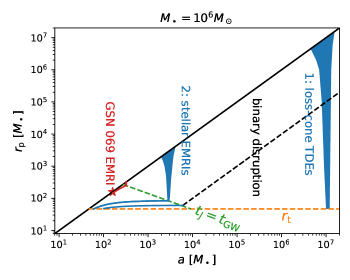
To analyze the formation rate of GSN 069 like EMRIs in the loss-cone channel, a diagram proposed in Ref. Linial and Sari (2023) is useful. As shown in Fig. 5, most stars are dominated by 2-body scatterings and get tidally disruption when scattered into a low-angular momentum orbit with , a small fraction of stars are scattered into the GW emission dominated regime (dubbed as stellar EMRIs) gradually circularising and finally lose mass via partial TDEs. The GSN 069 EMRI is one of the stellar EMRIs. The TDE rate/stellar EMRI formation rate can be estimated as
| (43) |
from which we find the ratio of the formation rate of GSN 069 like EMRIs to the total TDE rate as
| (44) |
where we have used the fact that only stars in the range of can possibly become GSN 069 like EMRIs (see Fig. 5). The ratio becomes even lower if considering the mass-segregation effect where the star density is expected to be suppressed at small radii Hopman and Alexander (2005); Preto and Amaro-Seoane (2010); Bar-Or and Alexander (2016); Babak et al. (2017); Amaro-Seoane (2018); Broggi et al. (2022). Therefore the stellar EMRI in GSN 069 unlikely comes from the loss-cone channel and similar analysis also applies to sBH EMRIs.
Hills mechanism has been proposed as an efficient EMRI formation channel, and the sBH EMRIs at coalescence from this channel was speculated to be nearly circular due to the long inspiral phase Miller et al. (2005). However recent simulations taking the mass segregation effect into account show that the orbital eccentricity of sBH EMRIs at coalescence actually peaks at high eccentricity, following a distribution similar to in the loss-cone channel Raveh and Perets (2021). For EMRIs in the earlier inspiral phase with orbital semi-major axis , the orbital eccentricity should be even higher, which is in contrast with low-eccentricity EMRI in GSN 069. From Fig. 5, the same conclusion can be obtained. In the Hills mechanism, the bounded stars after binary disruptions are highly eccentric with eccentricity Miller et al. (2005). The stars face the same two fates, and neither of them ends as GSN 069 like EMRIs: most stars end as loss-cone TDEs and the remaining small fractions of stars evolve into stellar EMRIs but they are too eccentric to become GSN 069 like EMRIs. And similar analysis also applies to sBH EMRIs.
In the wet EMRI formation channel, a SMO orbiting around an accreting SMBH can be captured to the accretion disk as interactions (dynamical friction and density waves) with the accretion disk tend to decrease to the orbital inclination angle w.r.t. the disk. After captured onto the disk, the SMO migrates inward driven by the density waves and gravitational wave emission. The orbital eccentricity is expected to be damped by the density waves to , where is the disk aspect ratio. The number of SMO captured is determined by
| (45) |
where is the capture rate of SMOs from the nuclear stellar cluster and is the migration velocity in the radial direction. The migration is dominated by the GW emission at small separations and by the type-I migration at large separations Pan and Yang (2021b), , with
| (46) |
and
| (47) |
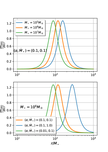
where , is the disk angular velocity, and is the disk aspect ratio Tanaka et al. (2002); Tanaka and Ward (2004). To obtain the SMO number , SMOs captured by the disk (disk component) and the residing the cluster (cluster component) should be evolved self-consistently (see e.g. Pan and Yang, 2021b; Pan et al., 2021; Pan and Yang, 2021a; Pan et al., 2022b). Here we focus on the distribution of disk-component SMOs in the vicinity of a SMBH (), where the capture rate is negligible and the distribution is clearly , in a steady state. As a result, we obtain in the GW emission dominated regime and in the type-I migration dominated regime for an -disk. In Fig. 6, we show the distributions for a few AGN examples, where in general peaks at for SMBHs with masses in the range of . After the AGN turns off, the SMOs will migrate inward driven solely by GW emissions and the distribution of SMOs in the radial direction will the reshaped with the peak moving outwards to a larger radius. Therefore, the EMRI in GSN 069 is consistent with the wet channel expectation.
In the above analysis, we did not take the tidal circularization process of the stellar orbit into account, which turns out to be subdominant. As shown in Ref. Verbunt and Phinney (1995), the tidal circularization rate of the stellar orbit around a SMBH is
| (48) | ||||
where is the mass of the stellar convective envelope and is the stellar effective temperature. In comparison with the circularization rate driven by GW emission Peters (1964),
| (49) | ||||
we find
| (50) | ||||
Therefore the tidal circularization never was dominant compared with the GW emission and can be safely ignored.
For the SMO settling down to a low-eccentricity orbit around the central SMBH, Kozai-Lidov oscillations driven by a third body must be quenched, e.g., by the apsidal precession of the SMO. The quench condition that the precession period is shorter than the Kozai-Lidov oscillation period has been derived as Blaes et al. (2002)
| (51) |
where and are the mass, the semi-major axis and the orbital eccentricity of the third body. For the EMRI system in GSN 069 with , the above condition is guaranteed as long as (and of course ). As shown in Ref. Liu et al. (2015), the maximum orbital eccentricity that could be excited turns out to be assuming an initial circular orbit and a stellar mass third object . Therefore Kozai-Lidov oscillations are not expected to drive the SMO off the low-eccentricity orbit.
To summarize, the low-eccentricity EMRI with semi-major axis (Eq. 34) in GSN 069 seems unlikely to be from the loss-cone channel or the Hills mechanism, and is consistent with the wet EMRI channel prediction.
IV.3 sBH EMRIs versus stellar EMRIs
In the EMRI+TDE disk model, the secondary object could be a normal star Linial and Metzger (2023a) or a sBH Franchini et al. (2023), which predict similar QPE properties and are not easy to be distinguished from current QPE observations (see the above two references for more detailed arguments). Identifying the nature of the secondary object will be invaluable for accurately predicting the rate of EMRIs detectable by spaceborne GW detectors and for distinguishing different accretion disk models in light of the increasing number of QPE detections.
Both models predict a decay in the orbital period due to energy loss in the collisions with different rates (see Eqs. (36,37)). The current constraint is not sufficiently accurate for distinguishing the two (see Eq. (33)). Longer monitoring the existing QPE sources is necessary in pinning down the orbital period decay rate , and consequently identifying the nature of the SMO.
Both models predict the strong-weak pattern in the QPE intensities, though with different dependence on the orbital eccentricity: and from Eqs. (2,4), therefore the strong-weak QPE intensity contrasts are or in these two models, respectively. For GSN 069, the intensity contrasts are roughly (see Fig. 1), which requires an orbital eccentricity for the sBH EMRI and for the stellar EMRI. The EMRI orbital eccentricity obtained from the QPE timing is at 2- confidence level, which favors the sBH EMRI. But this inference depends on the standard disk assumption, with the disk surface density , the accuracy of which is not yet confirmed for TDE disks. For example, in the disk model where Kocsis et al. (2011), the conclusion will be opposite. An important consequence of this dependence on the disk surface density profile is that the QPEs can be used as a probe to different accretion disk models as long as the nature of the SMO is confirmed, say, via the orbital change rate as explained in the previous paragraph.
In the above intensity analysis, we have implicitly assumed the symmetry of the emissions about the mid-plane of the disk after being shocked by the SMO from either direction, i.e., and , where denote the SMO moving directions and the denote the emission directions. The (approximate) symmetry has been verified in local simulations of sBH-disk collision Ivanov et al. (1998), but may not be true for star-disk collisions, where the emission could be preferably on one side of the post-collision disk due to the large geometrical size of the star. Such kind of asymmetry is indeed observed in our global HD simulations with different geometrical sizes of SMO colliding with the disk (see Appendix C for more details). Specially, with a large softening/sink particle radius to mimic the star-disk collision, the integrated density/temperature perturbations from the lower and upper disks behaves more asymmetric than the smaller softening case. But this kind of asymmetric is not as that strong as we expect. We suspect that this could be due to that we haven’t explore the extremely large geometry size contrast for these two scenarios, which is unlikely feasible in our global HD simulations.
IV.4 Model imitations and future work
In this work, we have been focusing on the analysis of the QPE source GSN 069. In principle, one can conduct a full parameter inference on the EMRI orbital model and the flare emission model. In fact, it is not straightforward to accurately model the QPE light curves with simple emission models. In this work, we used an expanding plasma ball model and a phenomenological model, both of which might be subject to some systematics in determining the flare starting times (see discussion about identifying possible systematics from HD simulations in Appendix C). To mitigate the impact of these potential systematics, we multiple the uncertainties by a scale factor in inferring the EMRI orbital parameters from the flare starting times. Another degree of freedom we did not consider in this work is the SMBH spin, which drives Lense-Thirring precession and consequently modulates the QPE recurrence times.
We will improve these model limitations and apply the improved analysis on all the existing QPE sources in a follow-up work, where the SMBH spin is straightforward to take into consideration in the EMRI orbits, and the emission model systematics may be improved with a simulation motivated model and/or a hierarchical inference method Isi et al. (2019) widely used in the GW community.
Acknowledgements.
We thank Liang Dai, Dong Lai and Bin Liu for enlightening discussions. Cong Zhou thanks Jialai Kang, Shifeng Huang, Giovanni Miniutti for helpful discussions on the X-ray data analysis and Qian Hu for valuable discussion. Lei Huang thanks for the support by National Natural Science Foundation of China (11933007,12325302), Key Research Program of Frontier Sciences, CAS (ZDBS-LY-SLH011), Shanghai Pilot Program for Basic Research-Chinese Academy of Science, Shanghai Branch (JCYJ-SHFY-2021-013). Y.P.L. is supported in part by the Natural Science Foundation of China (grants 12373070, and 12192223), the Natural Science Foundation of Shanghai (grant NO. 23ZR1473700). The calculations have made use of the High Performance Computing Resource in the Core Facility for Advanced Research Computing at Shanghai Astronomical Observatory. This paper made use of data from XMM-Newton, an ESA science mission with instruments and contributions directly funded by the ESA Member States and NASA.Appendix A Constraints on the parameters of the emission model and the flare timing model
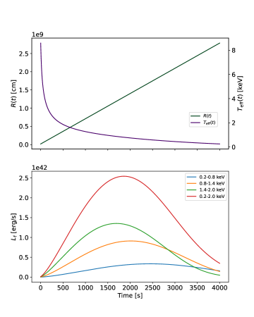
Fig. 7 displays the posterior corner plot of the plasma ball model parameters for the second flare in XMM 5. In Fig. 8, we show the evolution of the plasma ball size and the effective temperature , and its spectral evolution in the best-fit model of the second flare in XMM5. Around the peak of the QPE luminosity, the plasma ball effective temperature is keV, which is much higher than the observed value. This tension implies the limitation of the simple expanding plasma ball emission model. This is one of the reasons we consider an alternative phenomenological model for fitting the QPE light curves.
Fig. 9 displays the posterior corner plot of the EMRI orbital parameter constrained by the flare starting times shown in Table 1. All the angles defining the orbital plane orientation and the los direction are not well constrained saturating their priors, but the posteriors of the intrinsic orbital parameters yield import clues of the EMRI formation history as explained the Summary section.
Appendix B Scatter experiments of the remnant star and the SMO
If the new period in XMM 12 turns out to be largely different from those in the old regular phase and in the irregular phase, this new phase will pose a challenge to many existing models, including the EMRI+TDE disk model. There was some speculation that the shorter and are the result of a large change in the EMRI orbital ( decrease in the semi-major axis and increase in the eccentricity) after a close encounter with the remnant star at its pericenter during TDE 2. We examine this speculation by scattering experiments, and we find such large orbital change seems unlikely.
In order to test whether the orbital eccentricity of the SMO can be excited during the close encounter with the remnant star, we performed scatter experiments with N-body simulations to follow the orbital evolution of the sBH or the star during and after the TDE 2 event.
We use a 4th order Hermite integrator with block time step (Kokubo et al., 1998) to calculate the orbital evolution of the two bodies. We first consider the case where a remnant star that has experienced TDE 1 and a sBH are orbiting a SMBH. The mass of the remnant star, the sBH, and the SMBH are set to , , and respectively. The remnant star has a pericenter distance of and an orbital period of 9 years, which yields an eccentricity of 0.9954. The orbital inclination of the star is set to 0. The sBH has an initially low eccentricity of 0.05 and a semi-major axis of . The orbital inclination of the sBH is randomly chosen from 0 to . The other orbital elements (the longitude of ascending node, the argument of pericenter, and the time of pericenter passage) are randomly chosen from 0 to . We also consider the case where the remnant star encounters with another star instead of a sBH near the pericenter. In this case, the sBH is replaced by a star of . The orbital parameters remain unchanged.
In both cases, we integrate the system for roughly half an orbit of the remnant star to capture the orbital change of the SMO before and after the close encounter with the remnant star at the pericenter. A softening parameter is used for close encounter. 1000 simulations are performed in each case. No close encounters lead to a decrease in the orbital semi-major axis or a increase in the orbital eccentricity.
Appendix C HD simulations of SMO-disk collisions
We carry out a few 3D hydrodynamical simulations for the SMO-disk collision using Athena++ (Stone et al., 2020). The thin disk is initialized with an aspect ratio of , and an -viscosity (Shakura and Sunyaev, 1973) is implement with . For simplicity, the SMO collides with the disk around the central SMBH vertically. The SMO is initially far above the midplane such that the gravitational interaction between the SMO and the disk is weak. The motion of the SMO is prescribed by only vertical velocity while fixing cylindrical and azimuth location in time, where is the local Keplerian velocity.
The gravitational potential of the SMO is softened with the classical Plume potential with a softening scale of and the accretion of the SMO is modelled as a sink particle with the same softening radius . The softening/sink radius is to mimic the physical size of SMO. We adopt different softening/sink radii ( and ) to quantify the effect of the different physical size of SMO on the collision-induced emission, where is the Hill radius of the colliding object. With a mass ratio of , , this leads to and , respectively. A relative large mass SMO is adopted to save the computational cost as it is very challenging to well resolve the sink radius of the realistic mass ratio object even with grid refinement, e.g., . The softening scale adopted here is still too large compared to the size the sBH, which is extremely too small to simulate numerically. For stellar-mass black hole collision, the sink hole radius could be as small as the event horizon of the sBH, and orders of magnitude smaller than the Bondi/Hill radius of sBH. The case with a larger softening size is adopted for the case of star-disk collision, for which the physical size of star is usually much larger than the Bondi radius.
We evolve the gas adiabatically with an adiabatic index . The disk is resolved with a root grid of , where the radial domain is , and 3.5 disk scale height is modelled in the direction. Three levels of static refinement with a refine sphere of around the midplane is adopted to well resolve the collision location. As such, we can well resolve the Hill radius of the SMO with 40 grids in each dimension.
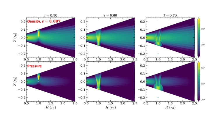
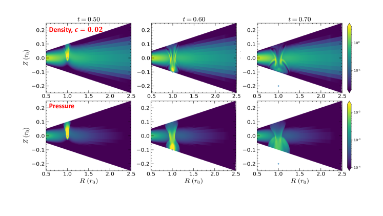
After the SMO-disk collision, there exists strong shocks which heat the gas around a narrow band of the collision site. By checking the vertical density and pressure distribution as shown in Fig. 11 and Fig. 12, the post-collision perturbation is asymmetric above and below the disk midplane. There is a dense blob above the midplanet before , i.e., prior to the collision at the midplane. The hot blob expands radially and vertically suffering from shearing motion of the disk, which can induce spiral arms in the disk. The perturbation then becomes stronger at the lower half plane of the disk, i.e., after the collision at the midplane. This asymmetric pattern is slightly stronger for the star-disk collision with a larger (at time of Fig. 11 and Fig. 12).
The shocked-heated dense blob will be responsible for the X-ray emission in observations. To quantify the emission features, we calculate the perturbed disk mass around the collision site , we integrate the disk mass from the upper and lower half of the disk for two different softening/sink radius, shown in Fig. 13. It is clearly seen that the perturbation is most prominent in the upper half of the disk before the collision and then becomes stronger later at the lower half of the disk. As expected, there is a time-delay between the peak of perturbed disk mass for the upper and lower disk, though this time delay may suffer from the boundary condition effect in the direction as we do not simulate the full domain of the disk. The difference of the integrated mass is not that large, although the local asymmetry of the density/pressure shown in Fig. 11 and Fig. 12 is stronger.
In addition, along the moving direction of the SMO, the burst actually consists of two components: a “precursor” burst at the moment of the shock breaking out the disk surface ( in Fig. 11 and Fig. 12) followed by a main burst sourced by the heated gas in the shocked column. In either light curve model, the former component is not modelled and is a possible reason of .
References
- Sun et al. (2013) Luming Sun, Xinwen Shu, and Tinggui Wang, “RX J1301.9+2747: A Highly Variable Seyfert Galaxy with Extremely Soft X-Ray Emission,” Astrophys. J. 768, 167 (2013), arXiv:1304.3244 [astro-ph.GA] .
- Giustini et al. (2020) Margherita Giustini, Giovanni Miniutti, and Richard D. Saxton, “X-ray quasi-periodic eruptions from the galactic nucleus of RX J1301.9+2747,” Astronomy&Astrophysics 636, L2 (2020), arXiv:2002.08967 [astro-ph.HE] .
- Arcodia et al. (2021) R. Arcodia, A. Merloni, K. Nandra, J. Buchner, M. Salvato, D. Pasham, R. Remillard, J. Comparat, G. Lamer, G. Ponti, A. Malyali, J. Wolf, Z. Arzoumanian, D. Bogensberger, D. A. H. Buckley, K. Gendreau, M. Gromadzki, E. Kara, M. Krumpe, C. Markwardt, M. E. Ramos-Ceja, A. Rau, M. Schramm, and A. Schwope, “X-ray quasi-periodic eruptions from two previously quiescent galaxies,” Nature (London) 592, 704–707 (2021), arXiv:2104.13388 [astro-ph.HE] .
- Arcodia et al. (2022) R. Arcodia, G. Miniutti, G. Ponti, J. Buchner, M. Giustini, A. Merloni, K. Nandra, F. Vincentelli, E. Kara, M. Salvato, and D. Pasham, “The complex time and energy evolution of quasi-periodic eruptions in eRO-QPE1,” Astronomy&Astrophysics 662, A49 (2022), arXiv:2203.11939 [astro-ph.HE] .
- Chakraborty et al. (2021) Joheen Chakraborty, Erin Kara, Megan Masterson, Margherita Giustini, Giovanni Miniutti, and Richard Saxton, “Possible X-Ray Quasi-periodic Eruptions in a Tidal Disruption Event Candidate,” Astroph.J.Lett. 921, L40 (2021), arXiv:2110.10786 [astro-ph.HE] .
- Wevers et al. (2022) T. Wevers, D. R. Pasham, P. Jalan, S. Rakshit, and R. Arcodia, “Host galaxy properties of quasi-periodically erupting X-ray sources,” Astronomy&Astrophysics 659, L2 (2022), arXiv:2201.11751 [astro-ph.HE] .
- Miniutti et al. (2023a) G. Miniutti, M. Giustini, R. Arcodia, R. D. Saxton, J. Chakraborty, A. M. Read, and E. Kara, “Alive and kicking: A new QPE phase in GSN 069 revealing a quiescent luminosity threshold for QPEs,” Astronomy&Astrophysics 674, L1 (2023a), arXiv:2305.09717 [astro-ph.HE] .
- Shu et al. (2018) X. W. Shu, S. S. Wang, L. M. Dou, N. Jiang, J. X. Wang, and T. G. Wang, “A Long Decay of X-Ray Flux and Spectral Evolution in the Supersoft Active Galactic Nucleus GSN 069,” Astroph.J.Lett. 857, L16 (2018), arXiv:1809.00319 [astro-ph.HE] .
- Sheng et al. (2021) Zhenfeng Sheng, Tinggui Wang, Gary Ferland, Xinwen Shu, Chenwei Yang, Ning Jiang, and Yang Chen, “Evidence of a Tidal-disruption Event in GSN 069 from the Abnormal Carbon and Nitrogen Abundance Ratio,” Astroph.J.Lett. 920, L25 (2021), arXiv:2109.01683 [astro-ph.GA] .
- Quintin et al. (2023) E. Quintin, N. A. Webb, S. Guillot, G. Miniutti, E. S. Kammoun, M. Giustini, R. Arcodia, G. Soucail, N. Clerc, R. Amato, and C. B. Markwardt, “Tormund’s return: Hints of quasi-periodic eruption features from a recent optical tidal disruption event,” Astronomy&Astrophysics 675, A152 (2023), arXiv:2306.00438 [astro-ph.HE] .
- Miniutti et al. (2023b) G. Miniutti, M. Giustini, R. Arcodia, R. D. Saxton, A. M. Read, S. Bianchi, and K. D. Alexander, “Repeating tidal disruptions in GSN 069: Long-term evolution and constraints on quasi-periodic eruptions’ models,” Astronomy&Astrophysics 670, A93 (2023b), arXiv:2207.07511 [astro-ph.HE] .
- Liu (2021) Tingting Liu, “Massive black holes flaring up time and again,” Nature Astronomy 5, 438–439 (2021).
- Raj and Nixon (2021) A. Raj and C. J. Nixon, “Disk Tearing: Implications for Black Hole Accretion and AGN Variability,” Astrophys. J. 909, 82 (2021), arXiv:2101.05825 [astro-ph.HE] .
- Pan et al. (2022a) Xin Pan, Shuang-Liang Li, Xinwu Cao, Giovanni Miniutti, and Minfeng Gu, “A Disk Instability Model for the Quasi-periodic Eruptions of GSN 069,” Astroph.J.Lett. 928, L18 (2022a), arXiv:2203.12137 [astro-ph.GA] .
- Pan et al. (2023) Xin Pan, Shuang-Liang Li, and Xinwu Cao, “Application of the Disk Instability Model to All Quasiperiodic Eruptions,” Astrophys. J. 952, 32 (2023), arXiv:2305.02071 [astro-ph.HE] .
- Kaur et al. (2023) Karamveer Kaur, Nicholas C. Stone, and Shmuel Gilbaum, “Magnetically dominated discs in tidal disruption events and quasi-periodic eruptions,” MNRAS 524, 1269–1290 (2023), arXiv:2211.00704 [astro-ph.HE] .
- Śniegowska et al. (2023) Marzena Śniegowska, Mikołaj Grzȩdzielski, Bożena Czerny, and Agnieszka Janiuk, “Modified models of radiation pressure instability applied to 10, 105, and 107 M⊙ accreting black holes,” Astronomy&Astrophysics 672, A19 (2023), arXiv:2204.10067 [astro-ph.HE] .
- Ingram et al. (2021) Adam Ingram, Sara E. Motta, Suzanne Aigrain, and Aris Karastergiou, “A self-lensing binary massive black hole interpretation of quasi-periodic eruptions,” MNRAS 503, 1703–1716 (2021), arXiv:2103.00017 [astro-ph.HE] .
- King (2020) Andrew King, “GSN 069 - A tidal disruption near miss,” MNRAS 493, L120–L123 (2020), arXiv:2002.00970 [astro-ph.HE] .
- King (2022) Andrew King, “Quasi-periodic eruptions from galaxy nuclei,” MNRAS 515, 4344–4349 (2022), arXiv:2206.04698 [astro-ph.GA] .
- King (2023) Andrew King, “Angular momentum transfer in QPEs from galaxy nuclei,” MNRAS 520, L63–L67 (2023), arXiv:2301.03582 [astro-ph.HE] .
- Chen et al. (2022) Xian Chen, Yu Qiu, Shuo Li, and F. K. Liu, “Milli-Hertz Gravitational-wave Background Produced by Quasiperiodic Eruptions,” Astrophys. J. 930, 122 (2022), arXiv:2112.03408 [astro-ph.HE] .
- Wang et al. (2022) Mengye Wang, Jinjing Yin, Yiqiu Ma, and Qingwen Wu, “A Model for the Possible Connection Between a Tidal Disruption Event and Quasi-periodic Eruption in GSN 069,” Astrophys. J. 933, 225 (2022), arXiv:2206.03092 [astro-ph.HE] .
- Zhao et al. (2022) Z. Y. Zhao, Y. Y. Wang, Y. C. Zou, F. Y. Wang, and Z. G. Dai, “Quasi-periodic eruptions from the helium envelope of hydrogen-deficient stars stripped by supermassive black holes,” Astronomy&Astrophysics 661, A55 (2022), arXiv:2109.03471 [astro-ph.HE] .
- Metzger et al. (2022) Brian D. Metzger, Nicholas C. Stone, and Shmuel Gilbaum, “Interacting Stellar EMRIs as Sources of Quasi-periodic Eruptions in Galactic Nuclei,” Astrophys. J. 926, 101 (2022), arXiv:2107.13015 [astro-ph.HE] .
- Lu and Quataert (2022) Wenbin Lu and Eliot Quataert, “Quasi-periodic eruptions from mildly eccentric unstable mass transfer in galactic nuclei,” arXiv e-prints , arXiv:2210.08023 (2022), arXiv:2210.08023 [astro-ph.HE] .
- Krolik and Linial (2022) Julian H. Krolik and Itai Linial, “Quasiperiodic Erupters: A Stellar Mass-transfer Model for the Radiation,” Astrophys. J. 941, 24 (2022), arXiv:2209.02786 [astro-ph.HE] .
- Linial and Sari (2023) Itai Linial and Re’em Sari, “Unstable Mass Transfer from a Main-sequence Star to a Supermassive Black Hole and Quasiperiodic Eruptions,” Astrophys. J. 945, 86 (2023), arXiv:2211.09851 [astro-ph.HE] .
- Suková et al. (2021) Petra Suková, Michal Zajaček, Vojtěch Witzany, and Vladimír Karas, “Stellar Transits across a Magnetized Accretion Torus as a Mechanism for Plasmoid Ejection,” Astrophys. J. 917, 43 (2021), arXiv:2102.08135 [astro-ph.HE] .
- Xian et al. (2021) Jingtao Xian, Fupeng Zhang, Liming Dou, Jiasheng He, and Xinwen Shu, “X-Ray Quasi-periodic Eruptions Driven by Star-Disk Collisions: Application to GSN069 and Probing the Spin of Massive Black Holes,” Astroph.J.Lett. 921, L32 (2021), arXiv:2110.10855 [astro-ph.HE] .
- Tagawa and Haiman (2023) Hiromichi Tagawa and Zoltán Haiman, “Flares from stars crossing active galactic nuclei disks on low-inclination orbits,” arXiv e-prints , arXiv:2304.03670 (2023), arXiv:2304.03670 [astro-ph.HE] .
- Linial and Metzger (2023a) Itai Linial and Brian D. Metzger, “EMRI + TDE = QPE: Periodic X-ray Flares from Star-Disk Collisions in Galactic Nuclei,” arXiv e-prints , arXiv:2303.16231 (2023a), arXiv:2303.16231 [astro-ph.HE] .
- Franchini et al. (2023) Alessia Franchini, Matteo Bonetti, Alessandro Lupi, Giovanni Miniutti, Elisa Bortolas, Margherita Giustini, Massimo Dotti, Alberto Sesana, Riccardo Arcodia, and Taeho Ryu, “Quasi-periodic eruptions from impacts between the secondary and a rigidly precessing accretion disc in an extreme mass-ratio inspiral system,” Astronomy&Astrophysics 675, A100 (2023), arXiv:2304.00775 [astro-ph.HE] .
- Miniutti et al. (2019) G. Miniutti, R. D. Saxton, M. Giustini, K. D. Alexander, R. P. Fender, I. Heywood, I. Monageng, M. Coriat, A. K. Tzioumis, A. M. Read, C. Knigge, P. Gandhi, M. L. Pretorius, and B. Agís-González, “Nine-hour X-ray quasi-periodic eruptions from a low-mass black hole galactic nucleus,” Nature (London) 573, 381–384 (2019), arXiv:1909.04693 [astro-ph.HE] .
- Linial and Metzger (2023b) Itai Linial and Brian D. Metzger, “Ultraviolet Quasi-periodic Eruptions from Star-Disk Collisions in Galactic Nuclei,” arXiv e-prints , arXiv:2311.16231 (2023b), arXiv:2311.16231 [astro-ph.HE] .
- Arnett (1980) W. D. Arnett, “Analytic solutions for light curves of supernovae of Type II,” Astrophys. J. 237, 541–549 (1980).
- Lehto and Valtonen (1996) Harry J. Lehto and Mauri J. Valtonen, “OJ 287 Outburst Structure and a Binary Black Hole Model,” Astrophys. J. 460, 207 (1996).
- Pihajoki (2016) P. Pihajoki, “Black hole accretion disc impacts,” MNRAS 457, 1145–1161 (2016), arXiv:1510.07642 [astro-ph.HE] .
- Jiang et al. (2022) Ning Jiang, Huan Yang, Tinggui Wang, Jiazheng Zhu, Zhenwei Lyu, Liming Dou, Yibo Wang, Jianguo Wang, Zhen Pan, Hui Liu, Xinwen Shu, and Zhenya Zheng, “Tick-Tock: The Imminent Merger of a Supermassive Black Hole Binary,” arXiv e-prints , arXiv:2201.11633 (2022), arXiv:2201.11633 [astro-ph.HE] .
- Ivanov et al. (1998) Pavel B. Ivanov, Igor V. Igumenshchev, and Igor D. Novikov, “Hydrodynamics of Black Hole-Accretion Disk Collision,” Astrophys. J. 507, 131–144 (1998).
- Shakura and Sunyaev (1973) N. I. Shakura and R. A. Sunyaev, “Black holes in binary systems. Observational appearance.” Astronomy&Astrophysics 24, 337–355 (1973).
- Kocsis et al. (2011) Bence Kocsis, Nicolás Yunes, and Abraham Loeb, “Observable signatures of extreme mass-ratio inspiral black hole binaries embedded in thin accretion disks,” Phys. Rev. D 84, 024032 (2011).
- Chandrasekhar (1943) S. Chandrasekhar, “Dynamical Friction. I. General Considerations: the Coefficient of Dynamical Friction.” Astrophys. J. 97, 255 (1943).
- Rephaeli and Salpeter (1980) Y. Rephaeli and E. E. Salpeter, “Flow past a massive object and the gravitational drag,” Astrophys. J. 240, 20–24 (1980).
- Binney and Tremaine (1987) James Binney and Scott Tremaine, Galactic dynamics (1987).
- Shankar et al. (1993) A. Shankar, W. Kley, and A. Burkert, “Axisymmetric accretion flow past large, gravitating bodies,” Astronomy&Astrophysics 274, 955 (1993).
- Ruffert and Arnett (1994) Maximilian Ruffert and David Arnett, “Three-dimensional Hydrodynamic Bondi-Hoyle Accretion. II. Homogeneous Medium at Mach 3 with gamma = 5/3,” Astrophys. J. 427, 351 (1994).
- Edgar (2004) Richard Edgar, “A review of Bondi-Hoyle-Lyttleton accretion,” New Astronomy Reviews 48, 843–859 (2004), arXiv:astro-ph/0406166 [astro-ph] .
- Chapon et al. (2013) Damien Chapon, Lucio Mayer, and Romain Teyssier, “Hydrodynamics of galaxy mergers with supermassive black holes: is there a last parsec problem?” MNRAS 429, 3114–3122 (2013), arXiv:1110.6086 [astro-ph.GA] .
- Thun et al. (2016) Daniel Thun, Rolf Kuiper, Franziska Schmidt, and Wilhelm Kley, “Dynamical friction for supersonic motion in a homogeneous gaseous medium,” Astronomy&Astrophysics 589, A10 (2016), arXiv:1601.07799 [astro-ph.GA] .
- Hunt (1971) R. Hunt, “A fluid dynamical study of the accretion process,” MNRAS 154, 141 (1971).
- Hunt (1979) R. Hunt, “Accretion of gas having specific heat ratio 3/3 by a moving gravitating body.” MNRAS 188, 83–91 (1979).
- Shima et al. (1985) E. Shima, T. Matsuda, H. Takeda, and K. Sawada, “Hydrodynamic calculations of axisymmetric accretion flow,” MNRAS 217, 367–386 (1985).
- Ruffert (1996) M. Ruffert, “Three-dimensional hydrodynamic Bondi-Hoyle accretion. V. Specific heat ratio 1.01, nearly isothermal flow.” Astronomy&Astrophysics 311, 817–832 (1996), arXiv:astro-ph/9510021 [astro-ph] .
- Norris et al. (2005) J. P. Norris, J. T. Bonnell, D. Kazanas, J. D. Scargle, J. Hakkila, and T. W. Giblin, “Long-Lag, Wide-Pulse Gamma-Ray Bursts,” Astrophys. J. 627, 324–345 (2005), arXiv:astro-ph/0503383 [astro-ph] .
- Chandrasekhar (1983) S. Chandrasekhar, The mathematical theory of black holes (1983).
- Shapiro (1964) Irwin I. Shapiro, “Fourth test of general relativity,” Phys. Rev. Lett. 13, 789–791 (1964).
- Speagle (2020) Joshua S. Speagle, “DYNESTY: a dynamic nested sampling package for estimating Bayesian posteriors and evidences,” MNRAS 493, 3132–3158 (2020), arXiv:1904.02180 [astro-ph.IM] .
- Williams (2021) Michael J. Williams, “nessai: Nested sampling with artificial intelligence,” (2021).
- Ashton et al. (2019) Gregory Ashton, Moritz Hübner, Paul D. Lasky, Colm Talbot, Kendall Ackley, Sylvia Biscoveanu, Qi Chu, Atul Divakarla, Paul J. Easter, Boris Goncharov, Francisco Hernandez Vivanco, Jan Harms, Marcus E. Lower, Grant D. Meadors, Denyz Melchor, Ethan Payne, Matthew D. Pitkin, Jade Powell, Nikhil Sarin, Rory J. E. Smith, and Eric Thrane, “BILBY: A User-friendly Bayesian Inference Library for Gravitational-wave Astronomy,” Astroph.J.S. 241, 27 (2019), arXiv:1811.02042 [astro-ph.IM] .
- Strüder et al. (2001) L. Strüder, U. Briel, K. Dennerl, R. Hartmann, E. Kendziorra, N. Meidinger, E. Pfeffermann, C. Reppin, B. Aschenbach, W. Bornemann, H. Bräuninger, W. Burkert, M. Elender, M. Freyberg, F. Haberl, G. Hartner, F. Heuschmann, H. Hippmann, E. Kastelic, S. Kemmer, G. Kettenring, W. Kink, N. Krause, S. Müller, A. Oppitz, W. Pietsch, M. Popp, P. Predehl, A. Read, K. H. Stephan, D. Stötter, J. Trümper, P. Holl, J. Kemmer, H. Soltau, R. Stötter, U. Weber, U. Weichert, C. von Zanthier, D. Carathanassis, G. Lutz, R. H. Richter, P. Solc, H. Böttcher, M. Kuster, R. Staubert, A. Abbey, A. Holland, M. Turner, M. Balasini, G. F. Bignami, N. La Palombara, G. Villa, W. Buttler, F. Gianini, R. Lainé, D. Lumb, and P. Dhez, “The European Photon Imaging Camera on XMM-Newton: The pn-CCD camera,” Astronomy&Astrophysics 365 (2001).
- Arnaud (1996) K. A. Arnaud, “XSPEC: The First Ten Years,” in Astronomical Data Analysis Software and Systems V, Astronomical Society of the Pacific Conference Series, Vol. 101, edited by George H. Jacoby and Jeannette Barnes (1996) p. 17.
- Patra et al. (2023) Kishore C. Patra, Wenbin Lu, Yilun Ma, Eliot Quataert, Giovanni Miniutti, Marco Chiaberge, and Alexei V. Filippenko, “Constraints on the narrow-line region of the x-ray quasi-periodic eruption source gsn 069,” (2023), arXiv:2310.05574 [astro-ph.HE] .
- Pan et al. (2022b) Zhen Pan, Zhenwei Lyu, and Huan Yang, “Mass-gap extreme mass ratio inspirals,” Phys. Rev. D 105, 083005 (2022b), arXiv:2112.10237 [astro-ph.HE] .
- Pan and Yang (2021a) Zhen Pan and Huan Yang, “Supercritical Accretion of Stellar-mass Compact Objects in Active Galactic Nuclei,” Astrophys. J. 923, 173 (2021a), arXiv:2108.00267 [astro-ph.HE] .
- Liska et al. (2018) M. Liska, C. Hesp, A. Tchekhovskoy, A. Ingram, M. van der Klis, and S. Markoff, “Formation of precessing jets by tilted black hole discs in 3D general relativistic MHD simulations,” MNRAS 474, L81–L85 (2018), arXiv:1707.06619 [astro-ph.HE] .
- Chatterjee et al. (2020) K. Chatterjee, Z. Younsi, M. Liska, A. Tchekhovskoy, S. B. Markoff, D. Yoon, D. van Eijnatten, C. Hesp, A. Ingram, and M. B. M. van der Klis, “Observational signatures of disc and jet misalignment in images of accreting black holes,” MNRAS 499, 362–378 (2020), arXiv:2002.08386 [astro-ph.GA] .
- Chatterjee et al. (2023) Koushik Chatterjee, Matthew Liska, Alexander Tchekhovskoy, and Sera Markoff, “Misaligned magnetized accretion flows onto spinning black holes: magneto-spin alignment, outflow power and intermittent jets,” arXiv e-prints , arXiv:2311.00432 (2023), arXiv:2311.00432 [astro-ph.HE] .
- Stone and Loeb (2012) Nicholas Stone and Abraham Loeb, “Observing Lense-Thirring Precession in Tidal Disruption Flares,” Phys. Rev. Lett. 108, 061302 (2012), arXiv:1109.6660 [astro-ph.HE] .
- Franchini et al. (2016) Alessia Franchini, Giuseppe Lodato, and Stefano Facchini, “Lense-Thirring precession around supermassive black holes during tidal disruption events,” MNRAS 455, 1946–1956 (2016), arXiv:1510.04879 [astro-ph.HE] .
- Linial and Quataert (2023) Itai Linial and Eliot Quataert, “Period Evolution of Repeating Transients in Galactic Nuclei,” arXiv e-prints , arXiv:2309.15849 (2023), arXiv:2309.15849 [astro-ph.HE] .
- Hopman and Alexander (2005) Clovis Hopman and Tal Alexander, “The Orbital Statistics of Stellar Inspiral and Relaxation near a Massive Black Hole: Characterizing Gravitational Wave Sources,” Astrophys. J. 629, 362–372 (2005), arXiv:astro-ph/0503672 [astro-ph] .
- Preto and Amaro-Seoane (2010) Miguel Preto and Pau Amaro-Seoane, “On Strong Mass Segregation Around a Massive Black Hole: Implications for Lower-Frequency Gravitational-Wave Astrophysics,” Astroph.J.Lett. 708, L42–L46 (2010), arXiv:0910.3206 [astro-ph.GA] .
- Bar-Or and Alexander (2016) Ben Bar-Or and Tal Alexander, “Steady-state Relativistic Stellar Dynamics Around a Massive Black hole,” Astrophys. J. 820, 129 (2016), arXiv:1508.01390 [astro-ph.GA] .
- Babak et al. (2017) Stanislav Babak, Jonathan Gair, Alberto Sesana, Enrico Barausse, Carlos F. Sopuerta, Christopher P. L. Berry, Emanuele Berti, Pau Amaro-Seoane, Antoine Petiteau, and Antoine Klein, “Science with the space-based interferometer LISA. V. Extreme mass-ratio inspirals,” Phys. Rev. D 95, 103012 (2017), arXiv:1703.09722 [gr-qc] .
- Amaro-Seoane (2018) Pau Amaro-Seoane, “Relativistic dynamics and extreme mass ratio inspirals,” Living Reviews in Relativity 21, 4 (2018), arXiv:1205.5240 [astro-ph.CO] .
- Broggi et al. (2022) Luca Broggi, Elisa Bortolas, Matteo Bonetti, Alberto Sesana, and Massimo Dotti, “Extreme mass ratio inspirals and tidal disruption events in nuclear clusters - I. Time-dependent rates,” MNRAS 514, 3270–3284 (2022), arXiv:2205.06277 [astro-ph.GA] .
- Miller et al. (2005) M. Coleman Miller, Marc Freitag, Douglas P. Hamilton, and Vanessa M. Lauburg, “Binary Encounters with Supermassive Black Holes: Zero-Eccentricity LISA Events,” Astroph.J.Lett. 631, L117–L120 (2005), arXiv:astro-ph/0507133 [astro-ph] .
- Raveh and Perets (2021) Yael Raveh and Hagai B. Perets, “Extreme mass-ratio gravitational-wave sources: mass segregation and post binary tidal-disruption captures,” MNRAS 501, 5012–5020 (2021), arXiv:2011.13952 [astro-ph.GA] .
- Pan and Yang (2021b) Zhen Pan and Huan Yang, “Formation rate of extreme mass ratio inspirals in active galactic nuclei,” Phys. Rev. D 103, 103018 (2021b), arXiv:2101.09146 [astro-ph.HE] .
- Pan et al. (2021) Zhen Pan, Zhenwei Lyu, and Huan Yang, “Wet extreme mass ratio inspirals may be more common for spaceborne gravitational wave detection,” Phys. Rev. D 104, 063007 (2021), arXiv:2104.01208 [astro-ph.HE] .
- Derdzinski and Mayer (2023) Andrea Derdzinski and Lucio Mayer, “In situ extreme mass ratio inspirals via subparsec formation and migration of stars in thin, gravitationally unstable AGN discs,” MNRAS 521, 4522–4543 (2023), arXiv:2205.10382 [astro-ph.GA] .
- Spitzer (1987) Lyman Spitzer, Dynamical evolution of globular clusters (1987).
- Tremaine et al. (2002) Scott Tremaine, Karl Gebhardt, Ralf Bender, Gary Bower, Alan Dressler, S. M. Faber, Alexei V. Filippenko, Richard Green, Carl Grillmair, Luis C. Ho, John Kormendy, Tod R. Lauer, John Magorrian, Jason Pinkney, and Douglas Richstone, “The Slope of the Black Hole Mass versus Velocity Dispersion Correlation,” Astrophys. J. 574, 740–753 (2002), arXiv:astro-ph/0203468 [astro-ph] .
- Gültekin et al. (2009) Kayhan Gültekin, Douglas O. Richstone, Karl Gebhardt, Tod R. Lauer, Scott Tremaine, M. C. Aller, Ralf Bender, Alan Dressler, S. M. Faber, Alexei V. Filippenko, Richard Green, Luis C. Ho, John Kormendy, John Magorrian, Jason Pinkney, and Christos Siopis, “The M- and M-L Relations in Galactic Bulges, and Determinations of Their Intrinsic Scatter,” Astrophys. J. 698, 198–221 (2009), arXiv:0903.4897 [astro-ph.GA] .
- Peters (1964) P. C. Peters, “Gravitational radiation and the motion of two point masses,” Phys. Rev. 136, B1224–B1232 (1964).
- Bahcall and Wolf (1976) J. N. Bahcall and R. A. Wolf, “Star distribution around a massive black hole in a globular cluster.” Astrophys. J. 209, 214–232 (1976).
- Tanaka et al. (2002) Hidekazu Tanaka, Taku Takeuchi, and William R. Ward, “Three-Dimensional Interaction between a Planet and an Isothermal Gaseous Disk. I. Corotation and Lindblad Torques and Planet Migration,” Astrophys. J. 565, 1257–1274 (2002).
- Tanaka and Ward (2004) Hidekazu Tanaka and William R. Ward, “Three-dimensional Interaction between a Planet and an Isothermal Gaseous Disk. II. Eccentricity Waves and Bending Waves,” Astrophys. J. 602, 388–395 (2004).
- Verbunt and Phinney (1995) F. Verbunt and E. S. Phinney, “Tidal circularization and the eccentricity of binaries containing giant stars.” Astronomy&Astrophysics 296, 709 (1995).
- Blaes et al. (2002) Omer Blaes, Man Hoi Lee, and Aristotle Socrates, “The Kozai Mechanism and the Evolution of Binary Supermassive Black Holes,” Astrophys. J. 578, 775–786 (2002), arXiv:astro-ph/0203370 [astro-ph] .
- Liu et al. (2015) Bin Liu, Diego J. Muñoz, and Dong Lai, “Suppression of extreme orbital evolution in triple systems with short-range forces,” MNRAS 447, 747–764 (2015), arXiv:1409.6717 [astro-ph.EP] .
- Isi et al. (2019) Maximiliano Isi, Katerina Chatziioannou, and Will M. Farr, “Hierarchical Test of General Relativity with Gravitational Waves,” Phys. Rev. Lett. 123, 121101 (2019), arXiv:1904.08011 [gr-qc] .
- Kokubo et al. (1998) Eiichiro Kokubo, Keiko Yoshinaga, and Junichiro Makino, “On a time-symmetric Hermite integrator for planetary N-body simulation,” Monthly Notices of the Royal Astronomical Society 297, 1067–1072 (1998), https://academic.oup.com/mnras/article-pdf/297/4/1067/3464608/297-4-1067.pdf .
- Stone et al. (2020) James M. Stone, Kengo Tomida, Christopher J. White, and Kyle G. Felker, “The Athena++ Adaptive Mesh Refinement Framework: Design and Magnetohydrodynamic Solvers,” Astroph.J.S. 249, 4 (2020), arXiv:2005.06651 [astro-ph.IM] .