A deep learning initialized iterative method for Navier-Stokes Darcy model

Abstract

A deep learning initialized iterative (Int-Deep) method is developed for numerically solving Navier-Stokes Darcy model. For this purpose, Newton iterative method is mentioned for solving the relative finite element discretized problem. It is proved that this method converges quadratically with the convergence rate independent of the finite element mesh size under certain standard conditions. Later on, a deep learning algorithm is proposed for solving this nonlinear coupled problem. Following the ideas of an earlier work by Huang, Wang and Yang (2020), an Int-Deep algorithm is constructed for the previous problem in order to further improve the computational efficiency. A series of numerical examples are reported to confirm that the Int-Deep algorithm converges to the true solution rapidly and is robust with respect to the physical parameters in the model.

1 Introduction

In the past twenty years, people have witnessed rapid progresses of deep learning (DL) methods in science and engineering (cf. [23]), leading to a revolution in computer science and its applications. With such an advance, various DL methods have been developed for solving all kinds of partial differential equations (PDEs). Such methods are mesh-free, quite different from the traditional mesh-based ones like finite difference methods, finite element methods, finite volume methods and so on. Firstly, deep neural networks (DNNs) are used to parameterize the solutions of PDEs. Then, the PDEs are reformulated as equivalent expected optimization problems according to variational principle, which are further discretized by Monte-Carlo methods. Finally, the network parameters are identified by solving the discrete problem with stochastic optimization algorithms. The remarkable advantage of the methods is that they can overcome the so-called “curse of dimensionality” (cf. [24]). More recent work (e.g. [29, 12, 34, 18]) has also shown that they are a valuable strategy to attack complicated mathematical physical problems in low dimensions, which are expensive to solve using traditional numerical methods. The weakness of the methods is that the number of iterations during learning process is usually very large or the accuracy is very limited (e.g., typically $10^{-2}$ to $10^{-4}$ relative error). Some typical DL methods include but not limited to the deep Ritz method [21], Physics-Informed Neural Networks methods (PINN) (cf. [37, 35, 41]), weak adversarial Networks [42] and the Friedrichs learning method [11]. The comprehensive introduction on applications of DL methods in computational mathematics can be found in [20].

We mention that the deep learning initialized iterative (Int-Deep) method is introduced in [30] for nonlinear variational problems. It is a hybrid iterative method, consisting of two phases. In the first phase, an expectation minimization problem formulated from a given nonlinear PDE is solved by mesh-free DL methods. In the second phase, the numerical solution from the first phase is interpolated as the initial guess, and some Newton-type iterative methods are used to solve the finite-dimensional problem discretized by finite element methods, which converges rapidly to the finite element solution. This method has been used successfully to solve semi-linear elliptic problems, linear and nonlinear eigenvalue problems (cf. [30]). The success of the method may rely partly on the so-called frequency principle mentioned in [39, 40], which asserts that DNNs tend to fit training data by a low-frequency function. This result implies that the DL solution with few iteration steps may capture the low frequency components of the exact solution, so it is reasonable to act as an initial guess of an iterative method for the variational problem under discussion.

In this paper, we intend to use the Int-Deep method to solve a nonlinear model$--$the Navier-Stokes Darcy model, which is widely applied in groundwater [10, 16, 33], flow in porous media [3, 2], industrial filtrations [25] and so on. Historically, the numerical solution of this nonlinear and coupled model attracts increasing attention. In [4, 15], the existence and local uniqueness of a weak solution are presented under suitable data restrictions. The well-posedness of the model is further studied in [22], with a simple and different proof. Following [22], Riviére et al. [13] compare and analyze two models which differ by the consideration of the inertial effects in the balance of forces on the interface. In [5, 17], Discacciati et al. formulate the coupled problem as an interface equation and analyze the associate (nonlinear) Steklov-Poincaré operators. With the development of the model, various numerical methods (e.g. [19, 36, 43]) have been employed to solve this model.

Our study in this paper is threefold. First of all, we analyze the convergence of Newton iterative method for the Navier-Stokes Darcy model discretized by mixed finite element methods. We note that the analysis in [5] is quite technical, which are obtained by reformulating the infinite dimensional coupled problem as an interface problem and using the Kantorovich theorem for Newton iterative method. Different from the previous approach, we derive the required result (cf. Theorem 3.1) in a straightforward way. A key observation is that an interface term in the Navier-Stokes equations, which is connected with Darcy equations, can be decomposed into a positive term plus an easily estimated term. Combining this finding with the analysis of Newton’s iteration for Navier-Stokes model in [28], we prove that the iterative method (cf. (3.1)-(3.3)) is convergent quadratically under certain standard conditions, with the convergence rate independent of the finite element mesh size $h$. Secondly, we design a PINN-type deep learning algorithm for the Navier-Stokes Darcy model, through expressing the unknowns with ResNet functions and constructing a log-loss function (see (4.1)) to improve computational efficiency. Thirdly, following the ideas in [30], we introduce the Int-Deep algorithm for the discrete Navier-Stokes Darcy model (cf. (2.6)-(2.7)). In other words, we solve the discrete problem by means of Newton iterative method, with the interpolation of the DNNs solution as an initial guess. Finally, a series of numerical examples are reported to confirm that the Int-Deep algorithm is able to reach the accuracy of the finite element method with few iteration steps. Furthermore, the algorithm shows good stability with variation of some parameters (such as the viscosity coefficient of fluid and the hydraulic conductivity tensor of the porous medium).

An outline of the paper is given as follows. In Section 2, we introduce the model problem and recall some results of the finite element method for the nonlinear coupled system. In Section 3, we discuss the stability and convergence of Newton iterative method under some conditions. In Section 4, a deep learning algorithm for the Navier-Stokes Darcy model is designed, and then the Int-Deep algorithm is developed for the Navier-Stokes Darcy model. In Section 5, we present some numerical examples to demonstrate the accuracy and efficiency of the Int-Deep algorithm.

2 The Navier-Stokes Darcy problem and its discretization

In this section, we aim to introduce the Navier-Stokes Darcy model and its finite element discretization. We also recall some important existing results which will be frequently used later on.

2.1 Navier-Stokes Darcy model

Let $\Omega\subset R^{d}~{}(d=2,~{}3)$ be a bounded polytopal domain, which is subdivided into a free fluid region $\Omega_{f}$ and a porous media region $\Omega_{p}$ by an interface $\Gamma$, as shown in Figure 1. Let $\Gamma_{f}=\partial\Omega_{f}\setminus\Gamma$ and $\Gamma_{p}=\partial\Omega_{p}\setminus\Gamma$ be the outer boundaries of the domains $\Omega_{f}$ and $\Omega_{p}$, respectively. Denote by $\bm{n}_{f}$ and $\bm{n}_{p}$ the unit outward normal vectors on $\partial\Omega_{f}$ and $\partial\Omega_{p}$, respectively. The unit tangential vector on $\Gamma$ is denoted by $\bm{\tau}$.

Figure 1: Domain schematic for Naiver-Stokes Darcy coupled flow.

The free flow in $\Omega_{f}$ is governed by the steady Navier-Stokes equations:

$$\begin{cases}-\operatorname{div}(\bm{T}(\bm{u},p))+\rho(\bm{u}\cdot\nabla)\bm{u}=\bm{f}_{f}&\text{in}~{}\Omega_{f},\\ \operatorname{div}\bm{u}=0&\text{in}~{}\Omega_{f},\end{cases}$$ (2.1)

where $\bm{u}$ and $p$ indicate the velocity field and the pressure field of the flow, respectively; $\nu>0$ stands for the viscosity coefficient, $\bm{T}(\bm{u},p)=2\nu\bm{D}(\bm{u})-p\bm{I}$ is the stress tensor, and $\bm{D}(\bm{u})=\frac{1}{2}\left(\nabla\bm{u}+\nabla^{{\rm T}}\bm{u}\right)$ is the deformation rate tensor; $\rho$ denotes the density of the flow and $\bm{f}_{f}$ is the external force.

The flow motion in the porous media region $\Omega_{p}$ is described by Darcy’s law:

$${}-\operatorname{div}(\bm{K}\nabla\varphi)=f_{p}\quad\text{in}~{}\Omega_{p},$$ (2.2)

where $\varphi$ is the hydraulic head, $f_{p}$ is a source term and $\bm{K}$ represents the hydraulic conductivity tensor. In this paper, we assume that $\bm{K}$ is symmetric $K_{ij}=K_{ji}$, and positive definite, i.e.

$$\alpha_{1}(\bm{x},\bm{x})\leq(\bm{K}\bm{x},\bm{x})\leq\alpha_{2}(\bm{x},\bm{x})\quad\forall\;\bm{x}\in~{}\Omega_{p},$$

for two positive constants $\alpha_{1}$ and $\alpha_{2}$.

The physical quantities are coupled on the interface $\Gamma$ through three interface conditions:

$$\begin{cases}\bm{u}\cdot\bm{n}_{f}=-\bm{K}\nabla\varphi\cdot\bm{n}_{f},\\ {\left[-\bm{T}(\bm{u},p)\bm{n}_{f}\right]\cdot\bm{n}_{f}=\rho g\varphi},\\ {\left[-\bm{T}(\bm{u},p)\bm{n}_{f}\right]\cdot\bm{\tau}_{j}=\frac{\nu\alpha}{\sqrt{\bm{\tau}_{j}\cdot\nu\bm{K}\cdot\bm{\tau}_{j}}}\bm{u}\cdot\bm{\tau}_{j},\;j=1,\ldots,d-1},\end{cases}$$ (2.3)

where $\left\{\bm{\tau}_{j}\right\}_{j=1}^{d-1}$ are linearly independent unit tangential vectors on $\Gamma$, and $\alpha$ is an experimentally determined positive parameter.

For simplicity, we consider homogeneous Dirichlet boundary conditions on the outer boundaries:

$$\begin{cases}\bm{u}=\bm{0}&\text{ on }\Gamma_{f},\\ \varphi=0&\text{ on }\Gamma_{p}.\end{cases}$$ (2.4)

In order to describe the variational formulation of this model, we have to introduce some function spaces in advance. Denote the admissible spaces for velocity, pressure and hydraulic head, respectively by

$$\bm{X}_{f} =\Big{\{}\bm{v}\in\bm{H}^{1}(\Omega_{f})=[H^{1}(\Omega_{f})]^{d}\mid\bm{v}=\bm{0}\text{ on }\Gamma_{f}\Big{\}},\qquad Q=L^{2}\left(\Omega_{f}\right),$$

$$X_{p} =\left\{\psi\in H^{1}\left(\Omega_{p}\right)\mid\psi=0\text{ on }\Gamma_{p}\right\}.$$

Then, the variational formulation of the coupled Navier-Stokes Darcy model $(\ref{model-pro1})-(\ref{model-pro4})$ is given as follows.

Find $\bm{u}\in\bm{X}_{f},\varphi\in X_{p}$ and $q\in Q$ such that

$$\begin{cases}&a_{f}(\bm{u},\bm{v})+a_{p}(\varphi,\psi)+a_{\Gamma}(\bm{u},\psi;\bm{v},\varphi)+c(\bm{u};\bm{u},\bm{v})+b(\bm{v},p)\\ &=(\bm{f}_{f},\bm{v})+\rho g(f_{p},\psi)~{}~{}~{}~{}\forall~{}\bm{v}\in\bm{X}_{f},\psi\in X_{p},\\ &b(\bm{u},q)=0~{}~{}~{}~{}\forall~{}q\in Q,\end{cases}$$ (2.5)

where,

$$a_{f}(\bm{u},\bm{v})=\int_{\Omega_{f}}2\nu\bm{D}(\bm{u}):\bm{D}(\bm{v})+\sum_{j=1}^{d-1}\frac{\nu\alpha}{\sqrt{\bm{\tau}_{j}\cdot\nu\bm{K}\bm{\tau}_{j}}}\int_{\Gamma}\left(\bm{u}\cdot\bm{\tau}_{j}\right)\left(\bm{v}\cdot\bm{\tau}_{j}\right),$$

$$a_{p}(\varphi,\psi)=\rho g\int_{\Omega_{p}}\bm{K}\nabla\varphi\cdot\nabla\psi,\quad a_{\Gamma}({\bm{u}},\psi;{\bm{v}},\varphi)=\rho g\int_{\Gamma}(\varphi\bm{v}-\psi\bm{u})\cdot\bm{n}_{f},$$

$$c(\bm{u};\bm{v},\bm{w})=\rho\int_{\Omega_{f}}(\bm{u}\cdot\nabla)\bm{v}\cdot\bm{w},\quad b(\bm{v},p)=-\int_{\Omega_{f}}p\operatorname{div}\bm{v},$$

$$(\bm{f}_{f},\bm{v})=\int_{\Omega_{f}}\bm{f}_{f}\cdot\bm{v},\quad(f_{p},\psi)=\int_{\Omega_{p}}f_{p}\psi.$$

Here and hereafter, we omit the infinitesimal element over an integration symbol when there is no confusion caused.

The existence and uniqueness of solution of $(\ref{weak-form-1})$ can be found in [22].

2.2 Finite element approximation

In this subsection, we shall give the finite element discretization of the Navier-Stokes Darcy model and review some existing results for subsequent analysis.

Let ${\mathcal{T}}_{f,h}$ (resp. ${\mathcal{T}}_{p,h}$) be a nondegenerate quasi-uniform triangulation of $\Omega_{f}$ (resp. $\Omega_{p}$). The partition ${\mathcal{T}}_{f,h}$ matches with the partition ${\mathcal{T}}_{p,h}$ at the interface $\Gamma$. Let ${\mathcal{T}}_{h}={\mathcal{T}}_{f,h}\cup{\mathcal{T}}_{p,h}$ be the partition of the whole domain $\Omega$. For each element $T\in{\mathcal{T}}_{h}$, we denote by $h_{T}$ the diameter of $T$; the mesh size of ${\mathcal{T}}_{h}$ is defined by $h=\max_{T\in{\mathcal{T}}_{h}}h_{T}$. Let $k$ be a non-negative integer, and denote by $P_{k}(T)$ the set of polynomials with the degree no more than $k$ on element $T\in{\mathcal{T}}_{h}$. Moreover, we use $C$ (with or without subscripts) to denote a generic positive constant independent of the mesh size $h$, which may take different values at different occurrences.

There are various combinations of the stable Stokes finite element pairs [7, 31] (such as MINI element, Taylor-Hood element, conforming Crouzeix-Raviart element) with continuous finite elements for Darcy equations. For convenience, we focus on the traditional Taylor-Hood element as an typical example in this paper. It is not difficult to extend the corresponding theory to other elements.

Define some finite element spaces by

$$\bm{X}_{f,h} = \{\bm{v}_{h}\in\bm{X}_{f},~{}\bm{v}_{h}|_{T}\in[P_{2}(T)]^{d}~{}\forall~{}T\in{\mathcal{T}}_{f,h}\},$$

$$Q_{h} = \{q_{h}\in Q\cap C^{0}(\Omega),~{}q_{h}|_{T}\in P_{1}(T)~{}\forall~{}T\in{\mathcal{T}}_{f,h}\},$$

$$X_{p,h} = \{\psi_{h}\in X_{p},~{}\psi_{h}|_{T}\in P_{2}(T)~{}\forall~{}T\in{\mathcal{T}}_{p,h}\}.$$

With these discrete function spaces, we give the finite element method for the coupled Navier-Stokes Darcy model $(\ref{model-pro1})-(\ref{model-pro4})$: Find $\bm{u}_{h}\in\bm{X}_{f,h}$, $p_{h}\in Q_{h}$, and $\varphi_{h}\in X_{p,h}$ such that

$$a_{f}(\bm{u}_{h},\bm{v}_{h})+a_{p}(\varphi_{h},\psi_{h})+a_{\Gamma}(\bm{u}_{h},\psi_{h};\bm{v}_{h},\varphi_{h})+c(\bm{u}_{h};\bm{u}_{h},\bm{v}_{h})+b(\bm{v}_{h},p_{h})$$ (2.6)

$$=(\bm{f}_{f},\bm{v}_{h})+\rho g(f_{p},\psi_{h})~{}~{}~{}~{}\forall~{}\bm{v}_{h}\in\bm{X}_{f,h},\;\psi_{h}\in X_{p,h},$$

$$b(\bm{u}_{h},q_{h})=0~{}~{}~{}~{}\forall~{}q_{h}\in Q_{h}.$$ (2.7)

To proceed with the forthcoming discussion about the well-posedness and convergence of the finite element method, we first recall some basic inequalities in Sobolev spaces as follows [1]. There exist constants $C_{p},~{}C_{t},~{}C_{k}$ and $C_{s}$ only depending on the domain $\Omega_{f}$, and $\tilde{C}_{p}$ and $\tilde{C}_{t}$ only depending on the domain $\Omega_{p}$, such that for all ${\bm{v}}\in\mathbf{X}_{f}$ and $\psi\in X_{p}$,

$$(\text{the Poincar\'{e} inequality})~{}~{}~{}~{}~{}~{} \|{\bm{v}}\|_{0,\Omega_{f}}\leq C_{p}|{\bm{v}}|_{1,\Omega_{f}},\hskip 42.67912pt\|\psi\|_{0,\Omega_{p}}\leq\tilde{C}_{p}|\psi|_{1,\Omega_{p}}.$$

$$(\text{the trace inequality})\hskip 39.83368pt \|{\bm{v}}\|_{0,\Gamma}\leq C_{t}|{\bm{v}}|_{1,\Omega_{f}},\hskip 49.79231pt\|\psi\|_{0,\Gamma}\leq\tilde{C}_{t}|\psi|_{1,\Omega_{p}}.$$

$$(\text{Korn's inequality})\hskip 51.21504pt |{\bm{v}}|_{1,\Omega_{f}}\leq C_{k}\|\bm{D}({\bm{v}})\|_{0,\Omega_{f}}.$$

$$(\text{the Sobolev inequality})\hskip 27.03003pt \|{\bm{v}}\|_{L^{6}(\Omega_{f})}\leq C_{s}|\nabla{\bm{v}}|_{1,\Omega_{f}}.$$

Using the Hölder inequality, the Sobolev inequality and Korn’s inequality, we immediately have (cf. [38])

$$c({\bm{u}};{\bm{v}},{\bm{w}})\leq\mathcal{N}_{d}\|{\bm{D}}({\bm{u}})\|_{0,\Omega_{f}}\|{\bm{D}}({\bm{v}})\|_{0,\Omega_{f}}\|{\bm{D}}({\bm{w}})\|_{0,\Omega_{f}},$$ (2.8)

with ${\mathcal{N}}_{d}$ depending only on $C_{s}$, $C_{k}$ and $d$.

In order to describe some important results, we define

$$\|\bm{f}_{f}\|_{*}=\frac{(\bm{f}_{f},{\bm{v}})}{\|{\bm{D}}({\bm{v}})\|_{0,\Omega_{f}}},\quad\|f_{p}\|_{*}=\frac{(f_{p},\psi)}{|\psi|_{1,\Omega_{p}}}.$$

The theoretical results given below indicate the well-posedness and convergence of the finite element method $(\ref{FEM-1})-(\ref{FEM-2})$. We refer the interesting readers to [9] for details along this line.

Theorem 2.1.

Assume that $\bm{f}_{f}\in[L^{2}(\Omega_{f})]^{d}$, $f_{p}\in L^{2}(\Omega_{p})$ and the viscosity coefficient $\nu$ satisfies

$$\nu^{\frac{3}{2}}\geq\sqrt{2}\mathcal{N}_{d}\mathcal{R},$$ (2.9)

with

$$\mathcal{R}=\left(\frac{1}{\nu}\|\bm{f}_{f}\|^{2}_{*}+\frac{\rho g}{\alpha_{1}}\|f_{p}\|^{2}_{*}\right)^{\frac{1}{2}}.$$ (2.10)

Then the finite element scheme $(\ref{FEM-1})-(\ref{FEM-2})$ has a unique solution satisfying the following estimate

$$2\nu\|\bm{D}({\bm{u}}_{h})\|^{2}_{0,\Omega_{f}}+\rho g\|\bm{K}\nabla\varphi_{h}\|^{2}_{0,\Omega_{p}}\leq\mathcal{R}^{2}.$$ (2.11)

Remark 1.

Under the assumption (2.9), it follows from (2.10) that

$$\|{\bm{D}}({\bm{u}}_{h})\|_{0,\Omega_{f}}\leq\frac{\nu}{2{\mathcal{N}}_{d}}.$$ (2.12)

Lemma 2.1.

There is a constant $\beta>0$ independent of $h$ such that

$$\inf_{q_{h}\in Q_{h}}\sup_{\bm{v}_{h}\in\bm{X}_{f,h}}\frac{b(\bm{v}_{s,h},q_{h})}{\|{\bm{D}}(\bm{v}_{h})\|_{0,\Omega_{f}}\|q_{h}\|_{0,\Omega_{f}}}\geq\beta.$$ (2.13)

Theorem 2.2.

Let $({\bm{u}},p,\varphi)$ be the solution of problem $(\ref{model-pro1})-(\ref{model-pro4})$ and $({\bm{u}}_{h},p_{h},\varphi_{h})$ be the solution of finite element scheme $(\ref{FEM-1})-(\ref{FEM-2})$. Assume that ${\bm{u}}\in\bm{H}^{3}(\Omega_{f})$, $p\in H^{2}(\Omega_{f})$ and $\varphi\in H^{3}(\Omega_{p})$. Then the following estimates hold:

$$2\nu \|{\bm{D}}({\bm{u}}-{\bm{u}}_{h})\|^{2}_{0,\Omega_{f}}+\sum_{j=1}^{d-1}\|({\bm{u}}-{\bm{u}}_{h})\cdot\bm{\tau}_{j}\|^{2}_{0,\Gamma}+\rho g\|{\bm{K}}^{\frac{1}{2}}\nabla(\varphi-\varphi_{h})\|^{2}_{0,\Omega_{p}}$$

$$\leq Ch^{4}(\|{\bm{u}}\|^{2}_{3,\Omega_{f}}+\|p\|^{2}_{2,\Omega_{f}}+\|\varphi\|^{2}_{3,\Omega_{p}}),$$ (2.14)

$$\|p -p_{h}\|^{2}\leq Ch^{4}(\|{\bm{u}}\|^{2}_{3,\Omega_{f}}+\|p\|^{2}_{2,\Omega_{f}}+\|\varphi\|^{2}_{3,\Omega_{p}}).$$ (2.15)

3 Newton’s Method for Navier-Stokes Darcy model

Newton iterative method and its theoretical analysis are the basis of our Int-Deep algorithm. In this section, we give Newton iterative method for solving Navier-Stokes Darcy model under the finite element discretization and provide stability and convergence analysis of the iterative method.

According to Newton iterative method for Navier-Stokes Darcy problems in infinite dimension (cf. [5]), its finite element analogue can be described as follows.

Given ${\bm{u}}^{h}_{0}\in X_{f,h}$, for $n\geq 1$, find ${\bm{u}}^{h}_{n}\in\bm{X}_{f,h}$, $p^{h}_{n}\in Q_{h}$ and $\varphi^{h}_{n}\in X_{p,h}$ such that

$$a_{f}({\bm{u}}^{h}_{n},{\bm{v}}_{h})+b({\bm{v}}_{h},p^{h}_{n})+\rho g\langle\varphi^{h}_{n},{\bm{v}}_{h}\cdot{\bm{n}}_{f}\rangle_{\Gamma}+c({\bm{u}}^{h}_{n};{\bm{u}}^{h}_{n-1},{\bm{v}}_{h})+c({\bm{u}}^{h}_{n-1};{\bm{u}}^{h}_{n},{\bm{v}}_{h})$$

$$=(\bm{f}_{f},{\bm{v}}_{h})+c({\bm{u}}^{h}_{n-1};{\bm{u}}^{h}_{n-1},{\bm{v}}_{h}),$$ (3.1)

$$b({\bm{u}}^{h}_{n},q_{h})=0,$$ (3.2)

$$a_{p}(\varphi^{h}_{n},\psi_{h})=\rho g\langle\psi_{h},{\bm{u}}^{h}_{n}\cdot{\bm{n}}_{f}\rangle_{\Gamma}+\rho g(f_{p},\psi_{h}),$$ (3.3)

for any $\bm{v}_{h}\in\bm{X}_{f,h},\;q_{h}\in Q_{h},\;\psi_{h}\in X_{p,h}$.

To analyze Newton iterative method, we next introduce two auxiliary problems given below.

For any $\zeta\in L^{2}(\Gamma)$ or $\eta\in L^{2}(\Omega_{p})$, find $\phi_{h}\in X_{p,h}$ such that

$$a_{p}(\phi_{h},\psi_{h})=\rho g\langle\zeta,\psi_{h}\rangle_{\Gamma}\quad\forall\;\psi_{h}\in X_{p,h},$$ (3.4)

or

$$a_{p}(\phi_{h},\psi_{h})=\rho g(\eta,\psi_{h})\quad\forall\;\psi_{h}\in X_{p,h}.$$ (3.5)

It is easy to prove by the Lax-Milgram lemma that problem $\eqref{aux-problem-darcy}$ or problem (3.5) has a unique solution, which induces a linear operator $\phi_{h}=T_{h}(\zeta)$ or $\phi_{h}=T_{h}(\eta)$. Furthermore, we have the following estimate which is easy to derive but important in our forthcoming analysis.

$$\|T_{h}(\eta)\|_{1,\Omega_{p}}\leq C_{r}\|\eta\|_{*},$$ (3.6)

with $C_{r}$ a positive constant independent of $h$.

The discussion on stability and convergence will be based on the following assumptions about the initial function ${\bm{u}}^{h}_{0}\in\bm{X}_{f,h}$ in Newton iterative method $\eqref{New-alg-1}-\eqref{New-alg-3}$:

$$2\nu\|{\bm{D}}({\bm{u}}^{h}_{0})\|_{0,\Omega_{f}} \leq C_{1}(\|\bm{f}_{f}\|_{*}+\|f_{p}\|_{*}),$$ (3.7)

$$\|{\bm{D}}({\bm{u}}_{h}-{\bm{u}}^{h}_{0})\|_{0,\Omega_{f}} \leq\frac{C_{1}}{\nu}\left(\|\bm{f}_{f}\|_{*}+\|f_{p}\|_{*}\right),$$ (3.8)

where

$$C_{1}=1+\rho gC_{r}\tilde{C}_{t}C_{t}C_{k}.$$

Lemma 3.1.

Assume the initial conditions (3.7)-(3.8) and the following stability condition hold:

$$\|\bm{f}_{f}\|_{*}+\|f_{p}\|_{*}\leq\frac{\nu^{2}}{9C_{1}{\mathcal{N}}_{d}}.$$ (3.9)

Then ${\bm{u}}^{h}_{m}$ defined by Newton iterative method $\eqref{New-alg-1}-\eqref{New-alg-3}$ satisfies

$$\|{\bm{D}}({\bm{u}}^{h}_{m})\|_{0,\Omega_{f}}\leq\frac{3C_{1}}{2\nu}\left(\|\bm{f}_{f}\|_{*}+\|f_{p}\|_{*}\right),$$ (3.10)

for all $m\geq 0$.

Proof.

We prove $\eqref{Newton-sta}$ by mathematical induction. The initial condition $\eqref{ini-con1}$ implies that $(\ref{Newton-sta})$ holds for $m=0$. Assuming that $(\ref{Newton-sta})$ holds for $m=J$ and we aim to prove the estimate holds for $m+1$. Taking $\zeta={\bm{u}}^{h}_{J+1}\cdot{\bm{n}}_{f}$ in $\eqref{aux-problem-darcy}$ gives $\phi^{b}_{J+1}=T_{h}({\bm{u}}^{h}_{J+1}\cdot{\bm{n}}_{f})$. Taking $\eta=f_{p}$ in $\eqref{aux-problem-2}$ gives $\phi^{i}$, which satisfies $\|\phi^{i}\|_{1,\Omega_{p}}\leq C_{r}\|f_{p}\|_{*}$ from $\eqref{aux-est-1}$. According to the superposition principle, $\varphi^{h}_{J+1}=\phi^{b}_{J+1}+\phi^{i}$ solves $(\ref{New-alg-3})$, which implies that

$$\rho g\langle\varphi^{h}_{J+1},{\bm{u}}^{h}_{J+1}\cdot{\bm{n}}_{f}\rangle_{\Gamma} =\rho g\langle\phi^{b}_{J+1},{\bm{u}}^{h}_{J+1}\cdot{\bm{n}}_{f}\rangle_{\Gamma}+\rho g\langle\phi^{i},{\bm{u}}^{h}_{J+1}\cdot{\bm{n}}_{f}\rangle_{\Gamma}$$

$$=a_{p}(T_{h}({\bm{u}}^{n}_{J+1}\cdot{\bm{n}}_{f}),\phi^{b}_{J+1})+\rho g\langle\phi^{i},{\bm{u}}^{h}_{J+1}\cdot{\bm{n}}_{f}\rangle_{\Gamma}$$

$$=a_{p}(\phi^{b}_{J+1},\phi^{b}_{J+1})+\rho g\langle\phi^{i},{\bm{u}}^{h}_{J+1}\cdot{\bm{n}}_{f}\rangle_{\Gamma}$$

$$\geq\rho g\langle\phi^{i},{\bm{u}}^{h}_{J+1}\cdot{\bm{n}}_{f}\rangle_{\Gamma}.$$ (3.11)

Taking $({\bm{v}}_{h},q_{h})=({\bm{u}}^{J+1}_{h},p^{J+1}_{h})\in\bm{X}_{f,h}\times Q_{h}$ in (3.1) with $n=J+1$ and using Korn’s inequality, the estimates $\eqref{tri-est}$, $\eqref{inter-est}$ and the induction assumption, we have

$$2\nu \|{\bm{D}}({\bm{u}}^{h}_{J+1})\|^{2}_{0,\Omega_{f}}$$

$$\leq (\bm{f}_{f},{\bm{u}}^{h}_{J+1})-\rho g\langle\varphi^{h}_{J+1},{\bm{u}}^{h}_{J+1}\cdot{\bm{n}}_{f}\rangle_{\Gamma}$$

$$+c({\bm{u}}^{h}_{J};{\bm{u}}^{h}_{J},{\bm{u}}^{h}_{J+1})-c({\bm{u}}^{h}_{J+1};{\bm{u}}^{h}_{J},{\bm{u}}^{h}_{J+1})-c({\bm{u}}^{h}_{J};{\bm{u}}^{h}_{J+1},{\bm{u}}^{h}_{J+1})$$

$$\leq \|\bm{f}_{f}\|_{*}\|{\bm{D}}({\bm{u}}^{h}_{J+1})\|_{0,\Omega_{f}}-\rho g\langle\phi^{i},{\bm{u}}^{h}_{J+1}\cdot{\bm{n}}_{f}\rangle_{\Gamma}$$

$$+{\mathcal{N}}_{d}\|{\bm{D}}({\bm{u}}^{h}_{J})\|^{2}_{0,\Omega_{f}}\|{\bm{D}}({\bm{u}}^{h}_{J+1})\|_{0,\Omega_{f}}+2{\mathcal{N}}_{d}\|{\bm{D}}({\bm{u}}^{h}_{J})\|_{0,\Omega_{f}}\|{\bm{D}}({\bm{u}}^{h}_{J+1})\|^{2}_{0,\Omega_{f}}$$

$$\leq C_{1}(\|\bm{f}_{f}\|_{*}+\|f_{p}\|_{*})\|{\bm{D}}({\bm{u}}^{h}_{J+1})\|_{0,\Omega_{f}}+\frac{9{\mathcal{N}}_{d}}{4\nu^{2}}C_{1}^{2}(\|\bm{f}_{f}\|_{*}+\|f_{p}\|_{*})^{2}\|{\bm{D}}({\bm{u}}^{h}_{J+1})\|_{0,\Omega_{f}}$$

$$+\frac{3{\mathcal{N}}_{d}}{\nu}C_{1}(\|\bm{f}_{f}\|_{*}+\|f_{p}\|_{*})\|{\bm{D}}({\bm{u}}^{h}_{J+1})\|^{2}_{0,\Omega_{f}}.$$

This, in conjunction with $(\ref{Newton-assume1})$, gives rise to

$$(\nu-\frac{\nu}{6})\|{\bm{D}}({\bm{u}}^{h}_{J+1})\|_{0,\Omega_{f}}\leq\frac{5}{4}C_{1}(\|\bm{f}_{f}\|_{*}+\|f_{p}\|_{*}),$$

which implies $(\ref{Newton-sta})$. ∎

Lemma 3.2.

The function ${\bm{u}}_{h}$ defined by the finite element method $(\ref{FEM-1})-(\ref{FEM-2})$ satisfies

$$\nu\|{\bm{D}}({\bm{u}}_{h})\|_{0,\Omega_{f}}\leq C_{1}(\|\bm{f}_{f}\|_{*}+\|f_{p}\|_{*}).$$ (3.12)

Proof.

Taking ${\bm{v}}_{h}={\bm{u}}_{h},~{}\psi_{h}=0$ in $(\ref{FEM-1})$ and noting that

$$b({\bm{u}}_{h},p_{h})=0,$$

we get

$$2\nu\|{\bm{D}}({\bm{u}}_{h})\|^{2}_{0,\Omega_{f}}=(\bm{f}_{f},{\bm{u}}_{h})-c({\bm{u}}_{h};{\bm{u}}_{h},{\bm{u}}_{h})-\langle\varphi_{h},{\bm{u}}_{h}\cdot{\bm{n}}_{f}\rangle_{\Gamma}.$$ (3.13)

In view of the estimates $(\ref{tri-est})$ and $(\ref{FEM-priori-est2})$, the trilinear from in the above equation can be bounded as

$$c({\bm{u}}_{h};{\bm{u}}_{h},{\bm{u}}_{h})\leq{\mathcal{N}}_{d}\|{\bm{D}}({\bm{u}}_{h})\|^{3}_{0,\Omega_{f}}\leq\frac{\nu}{2}\|{\bm{D}}({\bm{u}}_{h})\|^{2}_{0,\Omega_{f}}.$$ (3.14)

In order to handle the interface term $\langle\varphi_{h},{\bm{u}}_{h}\cdot{\bm{n}}_{f}\rangle_{\Gamma}$, taking ${\bm{v}}_{h}=0$ in $(\ref{FEM-1})$, we get

$$a_{p}(\varphi_{h},\psi_{h})=\rho g(f_{p},\psi_{h})+\langle{\bm{u}}_{h}\cdot{\bm{n}}_{f},\psi_{h}\rangle_{\Gamma}.$$ (3.15)

Applying a similar argument used for proving Lemma 3.1, we decompose $\varphi_{h}$ as $\varphi_{h}=\phi^{b}_{h}+\phi^{i}_{h}$, where $\phi^{b}_{h}$ is the solution of $(\ref{aux-problem-darcy})$ with $\zeta={\bm{u}}_{h}\cdot{\bm{n}}_{f}$, and $\phi^{i}_{h}$ is the solution of $(\ref{aux-problem-2})$ with $\eta=f_{p}$. Then, for the interface term, we have

$$\rho g\langle\varphi_{h},{\bm{u}}_{h}\cdot{\bm{n}}_{f}\rangle_{\Gamma} =\rho g\langle\phi^{b}_{h},{\bm{u}}_{h}\cdot{\bm{n}}_{f}\rangle_{\Gamma}+\rho g\langle\phi^{i}_{h},{\bm{u}}_{h}\cdot{\bm{n}}_{f}\rangle_{\Gamma}$$

$$=a_{p}(\phi^{b}_{h},\phi^{b}_{h})+\rho g\langle\phi^{i}_{h},{\bm{u}}_{h}\cdot{\bm{n}}_{f}\rangle_{\Gamma}$$

$$\geq\rho g\langle\phi^{i}_{h},{\bm{u}}_{h}\cdot{\bm{n}}_{f}\rangle_{\Gamma}.$$ (3.16)

The combination of $(\ref{FEM-solu-est-1})-(\ref{FEM-solu-est-2})$ implies the estimate $(\ref{FEM-solu-est})$. ∎

Finally, we derive error estimates of Newton iterative method. Let $({\bm{u}}_{h},\varphi_{h},p_{h})$ be the solution of the scheme $(\ref{FEM-1})-(\ref{FEM-2})$ and $({\bm{u}}^{h}_{n},p^{h}_{n},\varphi^{h}_{n})$ be the solution of Newton iterative method $(\ref{New-alg-1})-(\ref{New-alg-3})$. Set ${\bm{e}}^{u}_{n}={\bm{u}}_{h}-{\bm{u}}^{h}_{n},~{}e^{p}_{n}=p_{h}-p^{h}_{n}$ and $e^{\varphi}_{n}=\varphi_{h}-\varphi^{h}_{n}$.

Theorem 3.1.

Under the assumptions of Lemma 3.1, the following error estimates hold true.

$$\|{\bm{D}}({\bm{e}}^{u}_{n})\|_{0,\Omega_{f}} \leq\frac{C_{1}}{\nu}\left(\frac{3C_{1}{\mathcal{N}}_{d}}{2\nu^{2}}(\|\bm{f}_{f}\|_{*}+\|f_{p}\|_{*})\right)^{2^{n}-1}(\|\bm{f}_{f}\|_{*}+\|f_{p}\|_{*}),$$ (3.17)

$$|\nabla e^{\varphi}_{n}|_{1,\Omega_{p}} \leq\frac{\tilde{C}_{t}C_{t}C_{k}C_{1}}{\alpha_{1}\nu}\left(\frac{3C_{1}{\mathcal{N}}_{d}}{2\nu^{2}}(\|\bm{f}_{f}\|_{*}+\|f_{p}\|_{*})\right)^{2^{n}-1}(\|\bm{f}_{f}\|_{*}+\|f_{p}\|_{*}),$$ (3.18)

$$\|e^{p}_{n}\|_{0,\Omega_{f}} \leq(\frac{10}{3}+\frac{\tilde{C^{2}}_{t}C^{2}_{t}C^{2}_{k}}{\alpha_{1}\nu})\frac{C_{1}}{\beta}\left(\frac{3C_{1}{\mathcal{N}}_{d}}{2\nu^{2}}(\|\bm{f}_{f}\|_{*}+\|f_{p}\|_{*})\right)^{2^{n}-1}(\|\bm{f}_{f}\|_{*}+\|f_{p}\|_{*}),~{}~{}~{}~{}~{}$$ (3.19)

for all $n\geq 1$.

Proof.

Subtracting $(\ref{New-alg-1})-(\ref{New-alg-3})$ from the finite element scheme $(\ref{FEM-1})-(\ref{FEM-2})$, we find the error equations for Newton iterative method are determined by

$$a_{f}({\bm{e}}^{u}_{n},{\bm{v}}_{h})+a_{p}(e^{\varphi}_{n},\psi_{h})+b({\bm{v}}_{h},e^{p}_{n})+a_{\Gamma}({\bm{e}}^{u}_{n},\psi_{h};{\bm{v}}_{h},e^{\varphi}_{n})+c({\bm{e}}^{u}_{n};{\bm{u}}^{h}_{n-1},{\bm{v}}_{h})$$

$$+c({\bm{u}}^{h}_{n-1};{\bm{e}}^{u}_{h},{\bm{v}}_{h})+c({\bm{e}}^{u}_{n-1};{\bm{e}}^{u}_{n-1},{\bm{v}}_{h})=0~{}~{}~{}~{}\forall~{}\bm{v}_{h}\in\bm{X}_{f,h},\psi_{h}\in X_{p,h},$$ (3.20)

$$b({\bm{e}}^{u}_{n},q_{h})=0~{}~{}~{}~{}\forall~{}q_{h}\in Q_{h}.$$ (3.21)

Taking ${\bm{v}}_{h}={\bm{e}}^{u}_{n},~{}\psi_{h}=0$ in $(\ref{err-equ-1})$ and noting that $b({\bm{e}}^{u}_{n},e^{p}_{n})=0$, we achieve

$$2\nu\|{\bm{D}}({\bm{e}}^{u}_{n})\|^{2}_{0,\Omega_{f}} =-\rho g\langle e^{\varphi}_{n},{\bm{e}}^{u}_{n}\cdot{\bm{n}}_{f}\rangle_{\Gamma}-c({\bm{e}}^{u}_{n-1};{\bm{e}}^{u}_{n-1},{\bm{e}}^{u}_{n})-c({\bm{e}}^{u}_{n};{\bm{u}}^{h}_{n-1},{\bm{e}}^{u}_{n})-c({\bm{u}}^{h}_{n-1};{\bm{e}}^{u}_{n},{\bm{e}}^{u}_{n})$$

$$\leq{\mathcal{N}}_{d}\|{\bm{D}}({\bm{e}}^{u}_{n-1})\|^{2}_{0,\Omega_{f}}\|{\bm{D}}({\bm{e}}^{u}_{n})\|_{0,\Omega_{f}}+2{\mathcal{N}}_{d}\|{\bm{D}}({\bm{u}}^{h}_{n-1})\|_{0,\Omega_{f}}\|{\bm{D}}({\bm{e}}^{u}_{n})\|^{2}_{0,\Omega_{f}},$$

and with $(\ref{Newton-sta})$ and $(\ref{Newton-assume1})$, we further have

$$\|{\bm{D}}({\bm{e}}^{u}_{n})\|_{0,\Omega_{f}}\leq\frac{3{\mathcal{N}}_{d}}{2\nu}\|{\bm{D}}({\bm{e}}^{u}_{n-1})\|^{2}_{0,\Omega_{f}},$$ (3.22)

for $n\geq 1$.

Now, we prove $(\ref{Newton-err-est-1})$ by mathematical induction. It follows from the initial condition $\eqref{ini-con1}$ that (3.17) holds for $n=0$. Assuming that $(\ref{Newton-err-est-1})$ holds for $n=J$, we are going to prove that the estimate still holds for $n=J+1$. Applying the estimate $(\ref{Newton-iter-est})$ and the induction assumption gives

$$\|{\bm{D}}({\bm{e}}^{u}_{J+1})\|_{0,\Omega_{f}} \leq\frac{3{\mathcal{N}}_{d}}{2\nu}\|{\bm{D}}({\bm{e}}^{u}_{J})\|^{2}_{0,\Omega_{f}}$$

$$\leq\frac{3{\mathcal{N}}_{d}}{2\nu}\cdot\frac{C^{2}_{1}}{\nu^{2}}\left(\frac{3C_{1}{\mathcal{N}}_{d}}{2\nu^{2}}(\|\bm{f}_{f}\|_{*}+\|f_{p}\|_{*})\right)^{2^{J+1}-2}(\|\bm{f}_{f}\|_{*}+\|f_{p}\|_{*})^{2}$$

$$=\frac{C_{1}}{\nu}\left(\frac{3C_{1}{\mathcal{N}}_{d}}{2\nu^{2}}(\|\bm{f}_{f}\|_{*}+\|f_{p}\|_{*})\right)^{2^{J+1}-1}(\|\bm{f}_{f}\|_{*}+\|f_{p}\|_{*}),$$

which is $(\ref{Newton-err-est-1})$ with $n=J+1$. So we prove $(\ref{Newton-err-est-1})$ holds.

Let us consider the boundedness of $|e^{\varphi}_{n}|_{1}$. Taking ${\bm{v}}_{h}=\mathbf{0},~{}\psi_{h}=e^{\varphi}_{n}$ in $(\ref{err-equ-3})$ and applying $(\ref{Newton-err-est-1})$ gives

$$\alpha_{1}|\nabla e^{\varphi}_{n}|^{2}_{1,\Omega_{p}} \leq\|e^{\varphi}_{n}\|_{0,\Gamma}\|{\bm{e}}^{u}_{n}\|_{0,\Gamma}$$

$$\leq\tilde{C}_{t}|\nabla e^{\varphi}_{n}|_{1,\Omega_{p}}C_{t}C_{k}\|{\bm{D}}({\bm{e}}^{u}_{n})\|_{0,\Omega_{f}}$$

$$\leq\frac{\tilde{C}_{t}C_{t}C_{k}C_{1}}{\nu}|\nabla e^{\varphi}_{n}|_{1,\Omega_{p}}\left(\frac{3C_{1}{\mathcal{N}}_{d}}{2\nu^{2}}(\|\bm{f}_{f}\|_{*}+\|f_{p}\|_{*})\right)^{2^{n}-1}(\|\bm{f}_{f}\|_{*}+\|f_{p}\|_{*}).$$

Finally, we estimate $e^{p}_{n}$. By using the discrete inf-sup condition $\eqref{inf-sup}$, and the estimates $\eqref{Newton-sta}$, $(\ref{Newton-assume1})$, $\eqref{Newton-err-est-1}$ and $\eqref{Newton-err-est-2}$, we obtain

$$\beta \|e^{p}_{n}\|_{0,\Omega_{f}}$$

$$\leq 2\nu\|{\bm{D}}({\bm{e}}^{u}_{n})\|_{0,\Omega_{f}}+\rho gC_{t}\tilde{C}_{t}C_{k}|e^{\varphi}_{n}|_{1,\Omega_{p}}+2{\mathcal{N}}_{d}\|{\bm{D}}({\bm{u}}^{h}_{n-1})\|_{0,\Omega_{f}}\|{\bm{D}}({\bm{e}}^{u}_{n})\|_{0,\Omega_{f}}+{\mathcal{N}}_{d}\|{\bm{D}}({\bm{e}}^{u}_{n-1})\|^{2}_{0,\Omega_{f}}$$

$$\leq (2\nu+\frac{\nu}{3})\|{\bm{D}}({\bm{e}}^{u}_{n})\|_{0,\Omega_{f}}+\rho gC_{t}\tilde{C}_{t}C_{k}|e^{\varphi}_{n}|_{1,\Omega_{p}}+\frac{3}{2}{\mathcal{N}}_{d}\|{\bm{D}}({\bm{e}}^{u}_{n-1})\|^{2}_{0,\Omega_{f}}$$

$$\leq \frac{7C_{1}}{3}\left(\frac{3C_{1}{\mathcal{N}}_{d}}{2\nu^{2}}(\|\bm{f}_{f}\|_{*}+\|f_{p}\|_{*})\right)^{2^{n}-1}(\|\bm{f}_{f}\|_{*}+\|f_{p}\|_{*})$$

$$+\frac{\tilde{C}^{2}_{t}C^{2}_{t}C^{2}_{k}C_{1}}{\alpha_{1}\nu}\left(\frac{3C_{1}{\mathcal{N}}_{d}}{2\nu^{2}}(\|\bm{f}_{f}\|_{*}+\|f_{p}\|_{*})\right)^{2^{n}-1}(\|\bm{f}_{f}\|_{*}+\|f_{p}\|_{*})$$

$$+{C_{1}}\left(\frac{3C_{1}{\mathcal{N}}_{d}}{2\nu^{2}}(\|\bm{f}_{f}\|_{*}+\|f_{p}\|_{*})\right)^{2^{n}-1}(\|\bm{f}_{f}\|_{*}+\|f_{p}\|_{*})$$

$$= (\frac{10}{3}+\frac{\tilde{C}^{2}_{t}C^{2}_{t}C^{2}_{k}}{\alpha_{1}\nu}){C_{1}}\left(\frac{3C_{1}{\mathcal{N}}_{d}}{2\nu^{2}}(\|\bm{f}_{f}\|_{*}+\|f_{p}\|_{*})\right)^{2^{n}-1}(\|\bm{f}_{f}\|_{*}+\|f_{p}\|_{*}).$$

The proof is complete. ∎

Corollary 3.1.

The initial function ${\bm{u}}^{h}_{0}\in\bm{X}_{f,h}$ defined by the following finite element method for linear Stokes Darcy problem:

$$a_{f}({\bm{u}}^{h}_{0},{\bm{v}}_{h})+b({\bm{v}}_{h},p^{h}_{0})+\rho g\langle\varphi^{h}_{0},{\bm{v}}_{h}\cdot{\bm{n}}_{f}\rangle_{\Gamma}=(\bm{f}_{f},{\bm{v}}_{h})~{}~{}~{}~{}\forall~{}{\bm{v}}_{h}\in\bm{X}_{f,h},$$ (3.23)

$$b({\bm{u}}^{h}_{0},q_{h})=0~{}~{}~{}~{}\forall~{}q_{h}\in Q_{h},$$ (3.24)

$$a_{p}(\varphi^{h}_{0},\psi_{h})=\rho g\langle\psi_{h},{\bm{u}}^{h}_{0}\cdot{\bm{n}}_{f}\rangle_{\Gamma}+\rho g(f_{p},\psi_{h})~{}~{}~{}~{}\forall~{}\psi_{h}\in X_{p,h},$$ (3.25)

satisfies the initial condition (3.7)-(3.8).

Proof.

Taking $\zeta={\bm{u}}^{h}_{0}\cdot{\bm{n}}_{f}$ in auxiliary problem $\eqref{aux-problem-darcy}$ and $\eta=f_{p}$ in $(\ref{aux-problem-2})$, the corresponding solutions are denoted by $\phi^{b}_{0}$ and $\phi^{i}$, respectively. Then, we have $\phi^{b}_{0}=T_{h}({\bm{u}}^{h}_{0}\cdot{\bm{n}}_{f})$ and $\|\phi^{i}\|_{1,\Omega_{p}}\leq C_{r}\|f_{p}\|_{*}$. According to the superposition principle, we know that $\varphi^{h}_{0}=\phi^{b}_{0}+\phi^{i}$ solves $(\ref{Newton-ini-3})$, which implies that

$$\rho g\langle\varphi^{h}_{0},{\bm{v}}^{h}_{0}\cdot{\bm{n}}_{f}\rangle_{\Gamma} =\rho g\langle\phi^{b}_{0},{\bm{v}}^{h}_{0}\cdot{\bm{n}}_{f}\rangle_{\Gamma}+\rho g\langle\phi^{i},{\bm{v}}^{h}_{0}\cdot{\bm{n}}_{f}\rangle_{\Gamma}$$ (3.26)

$$=a_{p}(T_{h}({\bm{v}}^{h}_{0}\cdot{\bm{n}}_{f}),\phi^{b}_{0})+\rho g\langle\phi^{i},{\bm{v}}^{h}_{0}\cdot{\bm{n}}_{f}\rangle_{\Gamma}.$$

Taking ${\bm{v}}_{h}={\bm{u}}^{h}_{0}$ in $(\ref{Newton-ini-1})$, and using (3.26) and (3.6), we have

$$2\nu\|{\bm{D}}({\bm{u}}^{h}_{0})\|^{2}_{0,\Omega_{f}} \leq(\bm{f}_{f},{\bm{u}}^{h}_{0})-\rho g\langle\varphi^{h}_{0},{\bm{u}}^{h}_{0}\cdot{\bm{n}}_{f}\rangle_{\Gamma}$$ (3.27)

$$\leq(\bm{f}_{f},{\bm{u}}^{h}_{0})-a_{p}(\phi^{b}_{0},\phi^{b}_{0})-\rho g\langle\phi^{i},{\bm{u}}^{h}_{0}\cdot{\bm{n}}_{f}\rangle_{\Gamma}$$

$$\leq(\bm{f}_{f},{\bm{u}}^{h}_{0})-\rho g\langle\phi^{i},{\bm{u}}^{h}_{0}\cdot{\bm{n}}_{f}\rangle_{\Gamma}$$

$$\leq\|\bm{f}_{f}\|_{*}\|{\bm{D}}({\bm{u}}^{h}_{0})\|_{0,\Omega_{f}}+\rho gC_{r}\tilde{C}_{t}C_{t}C_{k}\|f_{p}\|_{*}\|{\bm{D}}({\bm{u}}^{h}_{0})\|_{0,\Omega_{f}}$$

$$\leq C_{1}(\|\bm{f}_{f}\|_{*}+\|f_{p}\|_{*})\|{\bm{D}}({\bm{u}}^{h}_{0})\|_{0,\Omega_{f}},$$

which yields $(\ref{ini-con1})$.

Next, we verify the initial condition $(\ref{ini-con2})$. Let ${\bm{u}}_{h},~{}\varphi_{h}$ be the solution of finite element scheme $(\ref{FEM-1})-(\ref{FEM-2})$. For convenience, set ${\bm{e}}^{u}_{0}={\bm{u}}_{h}-{\bm{u}}^{0}_{h}$, $e^{\varphi}_{0}=\varphi_{h}-\varphi^{0}_{h}$.

Subtracting $\eqref{Newton-ini-1}-\eqref{Newton-ini-3}$ from $\eqref{FEM-1}-\eqref{FEM-2}$ gives the error equations:

$$a_{f}({\bm{e}}^{u}_{0},{\bm{v}}_{h})+a_{p}(e^{\varphi}_{0},\psi_{h})+a_{\Gamma}({\bm{e}}^{u}_{0},\psi_{h};{\bm{v}}_{h},e^{\varphi}_{0})+b({\bm{v}}_{h},e^{p}_{0})+c({\bm{u}}_{h};{\bm{u}}_{h},{\bm{v}}_{h})=0,$$ (3.28)

$$b({\bm{e}}^{u}_{0},q_{h})=0,$$ (3.29)

for any ${\bm{v}}_{h}\in\bm{X}_{f,h},~{}\psi_{h}\in X_{p,h}$ and $q_{h}\in Q_{h}$.
Taking ${\bm{v}}_{h}={\bm{e}}^{u}_{0},~{}\psi_{h}=0$ in $(\ref{ini-err-equ-1})$ and noting that $b({\bm{e}}^{u}_{0},e^{p}_{0})=0$, we have

$$\nu\|{\bm{D}}({\bm{e}}^{u}_{0})\|^{2}_{0,\Omega_{f}}=-\rho g\langle e^{\varphi}_{0},{\bm{e}}^{u}_{0}\cdot{\bm{n}}_{f}\rangle_{\Gamma}-c({\bm{u}}_{h};{\bm{u}}_{h},{\bm{e}}^{u}_{0}).$$ (3.30)

Now, it suffices to estimate the terms on the right side of $\eqref{err-tool}$. Taking ${\bm{v}}_{h}=\mathbf{0}$, $\psi_{h}=e^{\varphi}_{0}$ in $(\ref{ini-err-equ-1})$ yields that

$$\rho g\langle{\bm{e}}^{u}_{0}\cdot{\bm{n}}_{f},e^{\varphi}_{0}\rangle_{\Gamma}=a_{p}(e^{\varphi}_{0},e^{\varphi}_{0})\geq 0.$$ (3.31)

Using the estimates $(\ref{tri-est})$ and $(\ref{FEM-solu-est})$ and the assumption $(\ref{Newton-assume1})$, we have

$$|c({\bm{u}}_{h};{\bm{u}}_{h},{\bm{e}}^{u}_{0})| \leq{\mathcal{N}}_{d}\|{\bm{D}}({\bm{u}}_{h})\|^{2}_{0,\Omega_{f}}\|{\bm{D}}({\bm{e}}^{u}_{0})\|_{0,\Omega_{f}}$$

$$\leq\frac{9{\mathcal{N}}_{d}C^{2}_{1}}{4\nu^{2}}\left(\|\bm{f}_{f}\|_{*}+\|f_{p}\|_{*}\right)^{2}\|{\bm{D}}({\bm{e}}^{u}_{0})\|_{0,\Omega_{f}}$$

$$\leq\frac{9{\mathcal{N}}_{d}C^{2}_{1}}{4\nu^{2}}\cdot\frac{\nu^{2}}{9C_{1}{\mathcal{N}}_{d}}\left(\|\bm{f}_{f}\|_{*}+\|f_{p}\|_{*}\right)\|{\bm{D}}({\bm{e}}^{u}_{0})\|_{0,\Omega_{f}}$$

$$\leq\frac{1}{4}C_{1}\left(\|\bm{f}_{f}\|_{*}+\|f_{p}\|_{*}\right)\|{\bm{D}}({\bm{e}}^{u}_{0})\|_{0,\Omega_{f}}.$$ (3.32)

By the estimates $\eqref{ini-err-sd1}$ and $\eqref{ini-err-sd2}$,

$$\|{\bm{D}}({\bm{e}}^{u}_{0})\|_{0,\Omega_{f}}\leq\frac{C_{1}}{4\nu}\left(\|\bm{f}_{f}\|_{*}+\|f_{p}\|_{*}\right).$$

which implies the initial condition $(\ref{ini-con2})$.

∎

4 The Int-Deep method

In this section, we first design a deep learning (DL) method for the Navier-Stokes Darcy model and then propose the Int-Deep algorithm, where the solution obtained from the DL method serves as an initial function for the Newton iteration method.

4.1 Deep learning method

In a DL method, the solution of a PDE is approximated by deep neural networks functions. In this work, we employ the classical residual neural network (ResNet) [27] to approximate the solutions of the Navier-Stokes Darcy model. For this purpose, we first recall its structure. Given an input $\bm{x}\in\mathbb{R}^{d}$, consider the following residual network architecture with skip connection in each layer.

$$\bm{h}_{0} =\bm{V}\bm{x},$$

$$\bm{g}_{l} =\sigma\left(\bm{W}_{l}\bm{h}_{l-1}+b_{l}\right),\;l=1,\ldots,L,$$

$$\bm{h}_{l} =\bm{h}_{l-1}+\bm{g}_{l},\hskip 34.14322ptl=1,\ldots,L,$$

$$\bm{\phi}(\bm{x};\bm{\tilde{\theta}}) =\bm{a}^{T}\bm{h}_{L},$$

where $\bm{\tilde{\theta}}=\{\bm{W}_{l},\bm{b}_{l},\bm{a}\},\bm{V}\in\mathbb{R}^{m\times d}$,

$$V(i,j)=\begin{cases}1&i=j,j\leq d\\ 0&\mathrm{otherwise}\end{cases},\;\bm{W}_{l}\in\mathbb{R}^{m\times m},\;\bm{b}_{l}\in\mathbb{R}^{m},$$

$\bm{a}\in\mathbb{R}^{m\times n}$, $L$ is the number of layers, $m$ is the width of the residual blocks and $\sigma$ is an activation function.

Next, we present the deep learning method in detail. Following the approach in [6], for the given essential boundary conditions ${\bm{u}}=\bm{g}_{{\bm{u}}}({\bm{x}}),\;{\bm{x}}\in\Gamma_{f},\;\varphi({\bm{x}})=g_{\varphi}({\bm{x}}),\;{\bm{x}}\in\Gamma_{p}$, we construct three neural network functions $\bm{\phi}_{\bm{u}}({\bm{x}};{\bm{\theta}}_{\bm{u}})$, $\phi_{p}({\bm{x}};{\bm{\theta}}_{p})$ and $\phi_{\varphi}({\bm{x}};{\bm{\theta}}_{\varphi})$ as follows.

$$\bm{\phi}_{\bm{u}}({\bm{x}};{\bm{\theta}}_{\bm{u}}) =B_{\bm{u}}({\bm{x}})\bm{N}_{\bm{u}}({\bm{x}};{\bm{\theta}}_{\bm{u}})+\bm{\bar{g}}_{{\bm{u}}}({\bm{x}}),$$

$$\phi_{p}({\bm{x}};{\bm{\theta}}_{p}) =N_{p}({\bm{x}};{\bm{\theta}}_{p}),$$

$$\phi_{\varphi}({\bm{x}};{\bm{\theta}}_{\varphi}) =B_{\varphi}({\bm{x}})N_{\varphi}({\bm{x}};{\bm{\theta}}_{\varphi})+\bar{g}_{\varphi}(\bm{x}),$$

where $B_{\bm{u}}({\bm{x}})$ and $B_{\varphi}(\bm{x})$ are two smooth scalar functions which satisfy the conditions $B_{\bm{u}}({\bm{x}})|_{\Gamma_{f}}=0$ and $B_{\varphi}(\bm{x})|_{\Gamma_{p}}=0$; $\bm{N}_{\bm{u}}({\bm{x}};{\bm{\theta}}_{\bm{u}})$, $N_{p}({\bm{x}};{\bm{\theta}}_{p})$ and $N_{\varphi}({\bm{x}};{\bm{\theta}}_{\varphi})$ are three distinct residual neural network functions; $\bm{\bar{g}_{u}}$ is the extension of $\bm{g_{u}}$ to $\Omega_{f}$, and $\bar{g}_{\varphi}$ is the extension of $g_{\varphi}$ to $\Omega_{p}$. Obviously, all the above neural network functions automatically satisfy the prescribed boundary conditions.

Setting ${\bm{\theta}}:=\{{\bm{\theta}}_{\bm{u}},{\bm{\theta}}_{p},{\bm{\theta}}_{\varphi}\}$, we respectively approximate $\bm{u}$, $p$ and $\varphi$ by

$${\bm{u}}({\bm{x}})\approx\bm{\phi}_{\bm{u}}({\bm{x}};{\bm{\theta}}_{\bm{u}}),\quad p({\bm{x}})\approx\phi_{p}({\bm{x}};{\bm{\theta}}_{p}),\quad\varphi\approx\phi_{\varphi}({\bm{x}};{\bm{\theta}}_{\varphi}),$$

with the network parameters determined by minimizing the $\log$ square loss

$$\bm{\theta^{*}}=\operatorname*{arg\,min}_{\bm{\theta}}\log_{2}(I(\bm{\phi}_{\bm{u}}({\bm{x}};{\bm{\theta}}_{\bm{u}}),\phi_{p}({\bm{x}};{\bm{\theta}}_{p}),\phi_{\varphi}({\bm{x}};{\bm{\theta}}_{\varphi}))+1),$$ (4.1)

where

$$I(\bm{u},p,\varphi)= \gamma_{1}\left(|\Omega_{f}|\mathbb{E}_{{\bm{\xi}}}\left(\left\|-\operatorname{div}{\bm{T}}\left({\bm{u}}({\bm{\xi}}),p({\bm{\xi}})\right)+\rho\left({\bm{u}}({\bm{\xi}})\cdot\nabla\right){\bm{u}}({\bm{\xi}})-\bm{f}_{f}({\bm{\xi}})\right\|^{2}+\left|\operatorname{div}{\bm{u}}({\bm{\xi}})\right|^{2}\right)\right.$$

$$\left.+|\Omega_{p}|\mathbb{E}_{\bm{\eta}}\left(\left|f_{p}(\bm{\eta})+\operatorname{div}(\bm{K}\nabla\varphi(\bm{\eta}))\right|^{2}\right)\right)$$

$$+\gamma_{2}\left(|\Gamma|\mathbb{E}_{\bm{\zeta}}\left(\left|{\bm{u}}(\bm{\zeta})\cdot\bm{n_{f}}+\bm{K}\nabla\varphi(\bm{\zeta})\cdot\bm{n}_{f}\right|^{2}\right.\right.$$

$$+||\bm{K}||_{2}\left|\left(\rho g\varphi(\bm{\zeta})+(\bm{T}({\bm{u}}(\bm{\zeta}),p(\bm{\zeta}))\bm{n}_{f})\cdot\bm{n}_{f})\right)\right|^{2}$$

$$+\sum_{j=1}^{d-1}\Big{(}\big{|}(\bm{T}({\bm{u}}(\bm{\zeta}),p(\bm{\zeta}))\bm{n}_{f})\cdot\bm{\tau}_{j}+\frac{\nu\alpha_{BJ}}{\sqrt{\bm{\tau}_{j}\cdot\nu\bm{K}\cdot\bm{\tau}_{j}}}{\bm{u}}(\bm{\zeta})\cdot\bm{\tau}_{j}\big{|}^{2}\Big{)}\bigg{)}.$$

Here $\gamma_{1}$, $\gamma_{2}$ are two positive parameters, $\|\cdot\|$ is the Euclidean norm of a vector, $\|\cdot\|_{2}$ is the 2-norm of a matrix, and $\bm{\xi},\bm{\eta},\bm{\zeta}$ are random variables that are uniformly distributed on $\Omega_{f},\;\Omega_{p}$ and $\Gamma$, respectively. Furthermore, we use the Monte-Carlo method to approximate the related expectation to derive the discretization of (4.1), which is solved by the stochastic gradient descent (SGD) method or its variants (e.g. Adam [32]).

With these preparations, the deep learning algorithm for Navier-Stokes Darcy model $(\ref{model-pro1})-(\ref{model-pro4})$ is described as Algorithm 1.

Algorithm 1 Deep learning method for Navier-Stokes Darcy problem.

Input: the maximum number of training $Epoch$, the learning rate $\eta$, sample size $N_{1},N_{2}$ and $N_{3}$.
Output:

$${\bm{u}}^{DL}=\bm{\phi}_{\bm{u}}({\bm{x}},{\bm{\theta}}_{\bm{u}}^{Epoch}),~{}~{}p^{DL}=\phi_{p}({\bm{x}},{\bm{\theta}}_{p}^{Epoch}),~{}~{}\varphi^{DL}=\phi_{\varphi}({\bm{x}},{\bm{\theta}}_{\varphi}^{Epoch}).$$

  Initialization: Let $l=0,~{}\eta^{0}=\eta$, the default initialization method in PyTorch is used to initialize the parameters of neural networks ${\bm{\theta}}_{\bm{u}}^{0},~{}{\bm{\theta}}_{\bm{p}}^{0},~{}{\bm{\theta}}_{\bm{\varphi}}^{0}$.

  while $l<Epoch$  do

      Generate independent random variables $\{\bm{\xi}_{i}\}_{i=1}^{N_{1}},\;\{\bm{\eta}_{i}\}_{i=1}^{N_{2}}$, and $\{\bm{\zeta}_{i}\}_{i=1}^{N_{3}}$ that are uniformly distributed on $\Omega_{f}$, $\Omega_{p}$, and $\Gamma$, respectively.

     Computing loss:

$$L=\log_{2}(I_{1}(\bm{\phi}_{\bm{u}}({\bm{\theta}}_{\bm{u}}^{l}),\phi_{p}({\bm{\theta}}_{p}^{l}),\phi_{\varphi}({\bm{\theta}}_{\varphi}^{l}))+1),$$ (4.2)

where

$$I_{1}({\bm{u}},p,\varphi)= \gamma_{1}\left(\frac{|\Omega_{f}|}{N_{1}}\sum_{i=1}^{N_{1}}(\left\|-\operatorname{div}\bm{T}\left({\bm{u}}({\bm{\xi}}_{i}),p({\bm{\xi}}_{i})\right)+\rho\left({\bm{u}}({\bm{\xi}}_{i})\cdot\nabla\right){\bm{u}}({\bm{\xi}}_{i})-\bm{f}_{f}({\bm{\xi}}_{i})\right\|^{2}+\left|\operatorname{div}{\bm{u}}({\bm{\xi}}_{i})\right|^{2})\right.$$

$$\left.+\frac{|\Omega_{p}|}{N_{2}}\sum_{i=1}^{N_{2}}\left(\left|f_{p}({\bm{\eta}}_{i})+\operatorname{div}(\bm{K}\nabla\varphi({\bm{\eta}}_{i}))\right|^{2}\right)\right)$$

$$+\gamma_{2}\bigg{(}\frac{|\Gamma|}{N_{3}}\sum_{i=1}^{N_{3}}(\big{|}{\bm{u}}(\bm{\zeta}_{i})\cdot\bm{n}_{f}+\bm{K}\nabla\varphi(\bm{\zeta}_{i})\cdot\bm{n}_{f}\big{|}^{2}$$

$$+||\bm{K}||_{2}\big{|}\left(\rho g\varphi(\bm{\zeta}_{i})+(\bm{T}({\bm{u}}(\bm{\zeta}_{i}),p(\bm{\zeta}_{i}))\bm{n}_{f})\cdot\bm{n}_{f})\right)\big{|}^{2}$$

$$+\sum_{j=1}^{d-1}\Big{(}\big{|}(\bm{T}({\bm{u}}(\bm{\zeta}_{i}),p(\bm{\zeta}_{i}))\bm{n}_{f})\cdot\bm{\tau}_{j}+\frac{\nu\alpha_{BJ}}{\sqrt{\bm{\tau}_{j}\cdot\nu\bm{K}\cdot\bm{\tau}_{j}}}{\bm{u}}(\bm{\zeta}_{i})\cdot\bm{\tau}_{j}\big{|}^{2}\Big{)}\bigg{)}.$$

     Updating parameters ${\bm{\theta}}_{\bm{u}}^{l+1}={\bm{\theta}}_{\bm{u}}^{l}-\eta^{l}\nabla_{\bm{{\bm{\theta}}_{\bm{u}}}}L,~{}{\bm{\theta}}_{p}^{l+1}={\bm{\theta}}_{p}^{l}-\eta^{l}\nabla_{\bm{{\bm{\theta}}_{p}}}L,~{}{\bm{\theta}}_{\varphi}^{l+1}={\bm{\theta}}_{\varphi}^{l}-\eta^{l}\nabla_{\bm{{\bm{\theta}}_{\varphi}}}L.$

     Let $l=l+1.$

  end while

4.2 The Int-Deep method for solving the Navier-Stokes Darcy problem

Since Newton iterative method is only locally convergent, it is very challenging to choose reasonably an initial guess. One natural choice is taking the initial guess as the solutions to the Stokes Darcy model (cf. (3.23)-(3.25)). However, the convergence is very sensitive to the physical parameters in the model. Motivated by the ideas in [30], we are tempted to choose $I_{h}{\bm{u}}^{DL}$ as an initial guess, where ${\bm{u}}^{DL}$ denotes the deep learning solution obtained from Algorithm 1 with few iteration steps, and $I_{h}$ is the usual nodal interpolation operator (cf. [8, 14]). Similar to [30], this method is referred to as the Int-Deep method for the Navier-Stokes Darcy problem $(\ref{model-pro1})-(\ref{model-pro4})$, and is described as Algorithm 2. It is worthy to emphasize that the later choice may rely partly on the so-called frequency principle mentioned in [39, 40], which asserts that DNNs tend to fit training data by a low-frequency function. This result implies that the DL solution with few iteration is a good approximate solution which may capture the low-frequency components of the exact solution, so it is reasonable to choose it as an initial guess. Our numerical results also indicate the superiority of such a choice.

Algorithm 2 Int-Deep method for Navier-Stokes Darcy problem.

Input: the target accuracy $\epsilon$, the maximum number of iterations $N_{\max}$, the approximate solution in a form of a DNN ${\bm{u}}^{DL}$.
Output: $\bm{u}^{h}_{ID}=\bm{u}^{h}_{n},\;p^{h}_{ID}=p_{n}^{h},\;\varphi^{h}_{ID}=\varphi^{h}_{n}$.

  Initialization: Let $\bm{u}_{0}^{h}={I_{h}{\bm{u}}^{DL}}$, $n=1$, and $e_{0}=1$.

  while $e_{n-1}>\epsilon$ and $n\leq N_{\max}$ do

      find ${\bm{u}}^{h}_{n}\in\mathbf{X}_{f,h},\;p^{h}_{n}\in Q_{h}$, and $\varphi^{h}_{n}\in X_{p}$ such that

$$a_{f}({\bm{u}}^{h}_{n},{\bm{v}}_{h})+b({\bm{v}}_{h},p^{h}_{n})+\rho g\langle\phi^{h}_{n},{\bm{v}}_{h}\cdot{\bm{n}}_{f}\rangle_{\Gamma}+c({\bm{u}}^{h}_{n};{\bm{u}}^{h}_{n-1},{\bm{v}}_{h})+c({\bm{u}}^{h}_{n-1};{\bm{u}}^{h}_{n},{\bm{v}}_{h})$$

$$=(\bm{f}_{f},{\bm{v}}_{h})+c({\bm{u}}^{h}_{n-1};{\bm{u}}^{h}_{n-1},{\bm{v}}_{h}),$$

$$b({\bm{u}}^{h}_{n},q_{h})=0,$$

$$a_{p}(\varphi^{h}_{n},\psi_{h})=\rho g\langle\psi_{h},{\bm{u}}^{h}_{n}\cdot{\bm{n}}_{f}\rangle_{\Gamma}+\rho g(f_{p},\psi_{h}).$$

     $e_{n}=\max(\frac{\|\bm{u}_{n}^{h}-\bm{u}_{n-1}^{h}\|_{0,\Omega_{f}}}{\|\bm{u}_{n-1}^{h}\|_{0,\Omega_{f}}},\frac{\|\varphi_{n}^{h}-\varphi_{n-1}^{h}\|_{0,\Omega_{p}}}{\|\varphi_{n-1}^{h}\|_{0,\Omega_{p}}},\frac{\|p_{n}^{h}-p_{n-1}^{h}\|_{0,\Omega_{f}}}{\|p_{n-1}^{h}\|_{0,\Omega_{f}}}$), $n=n+1$.

  end while

5 Numerical experiments

In this section, we shall present some numerical experiments to illustrate the performance of Algorithm 1 and Algorithm 2 for Navier-Stokes Darcy problem.

The specific details about the implementation of algorithms are provided in advance. In Algorithm 1, we use ResNets of width 50, depth 5 for the Navier-Stokes problem and width 50, depth 6 for the Darcy problem. the activation function in all neural networks is taken as $\sigma=\max\{x^{3},~{}0\}$. During the training process, we train the neural networks using the Adam optimizer [32] with a learning rate of $\eta=5\text{e}-03$. The learning rate decays exponentially and the decay rate is $0.01^{\frac{1}{10000}}$. The batch size is taken as: $N_{1}=N_{2}=1024$, $N_{3}=256$ for all 2D examples; $N_{1}=N_{2}=3000$, $N_{3}=512$ for the 3D example. In Algorithm 2, we set $N_{\max}=20$, $\epsilon=1e-7$ for all examples.

Some notations in the following part are summarized here. In numerical experiments, different strategies are employed to generate initial guesses for Newton iterative method, and corresponding results will be compared with the Int-Deep algorithm. We will refer to $\bm{u}^{DL}_{0}$ as the initial guess $I_{h}\bm{u}^{DL}$ where $\bm{u}^{DL}$ is provided by Algorithm 1 with 200 epochs in the Adam, $\bm{u}^{SD}_{0}$ as the initial guess obtained by solving the discretized Stokes Darcy problem (3.23) -(3.25), and $\bm{C}$ as the initial value which is a constant $C$. The number of epochs in the Adam for deep learning method is denoted by $\#$Epoch and the number of iterations in Newton iterative method is denoted by $\#\mathrm{K}$. The accuracy of the solution of Algorithm 1 is measured by the discrete maximum norm: for any $v\in C(\bar{\Omega})$,

$$\|v\|_{0,\infty,h}=\max_{x\in\Omega_{h}}|{\bm{v}}({\bm{x}})|,~{}~{}\Omega_{h}\text{~{}is the set of all vertices in~{}}\mathcal{T}_{h}.$$

We measure the accuracy of solution of Algorithm 2 by the relative $L^{2}$-error and $H^{1}$-error:

$$\begin{array}[]{llll}\|\bm{e}_{\bm{u}}^{h}\|_{0}=\frac{\left\|\bm{u}-\bm{u}^{h}_{ID}\right\|_{0,\Omega_{f}}}{\left\|\bm{u}\right\|_{0,\Omega_{f}}},&\|e_{p}^{h}\|_{0}=\frac{\left\|p-p^{h}_{ID}\right\|_{0,\Omega_{f}}}{\left\|p\right\|_{0,\Omega_{f}}},&\|e^{\varphi_{h}}_{h}\|_{0}=\frac{\left\|\varphi_{h}-\varphi^{h}_{ID}\right\|_{0,\Omega_{p}}}{\left\|\varphi\right\|_{0,\Omega_{p}}},\\ \|\bm{e}_{\bm{u}}^{h}\|_{1}=\frac{\left|\bm{u}-\bm{u}^{h}_{ID}\right|_{1,\Omega_{f}}}{\left|\bm{u}\right|_{1,\Omega_{f}}},&\|e^{h}_{\varphi}\|_{1}=\frac{\left|\varphi-\varphi^{h}_{ID}\right|_{1,\Omega_{p}}}{\left|\varphi\right|_{1,\Omega_{p}}}.&\end{array}$$

5.1 A 2D–example with a closed-form solution

In this example, we consider the coupled problem $(\ref{model-pro1})-(\ref{model-pro4})$ in $\Omega\in\mathbb{R}^{2}$ with $\Omega_{f}=(0,\pi)\times(0,\pi),\;\Omega_{p}=(0,\pi)\times$ $(-\pi,0)$ and the interface $\Gamma=(0,\pi)\times\{0\}$. The exact solution is given by

$$\begin{cases}u=2\sin y\cos y\cos x&\text{ in }\Omega_{f},\\ v=\left(\sin^{2}y-2\right)\sin x&\text{ in }\Omega_{f},\\ p=\sin x\sin y+\frac{1}{3\kappa},&\text{ in }\Omega_{f},\\ \varphi=\frac{1}{\kappa}(\left(e^{y}-e^{-y}\right)\sin x+\frac{1}{3})&\text{ in }\Omega_{p},\end{cases}$$

where the components of $\bm{u}$ are denoted by $(u,v)$ for convenience. For simplicity, all the parameters except $\nu$ and $\kappa~{}(\bm{K}=\kappa\bm{I})$ in the coupled model are set to be 1. In (4.2), we set $\gamma_{1}=200,\;\gamma_{2}=1$; $B_{\bm{u}}({\bm{x}})=x(x-\pi)(y-\pi)$ and $B_{\varphi}(\bm{x})=x(x-\pi)(y+\pi)$. To evaluate the test error of deep learning method, we adopt a mesh size $h=\frac{1}{1024}$ to generate the uniform triangulation $\mathcal{T}_{h}$ as the test locations.

5.1.1 The Performance of Algorithm 1

In this part, we focus on the performance of Algorithm 1 and the results are presented in Table $\ref{tab:DLnu=1K=1}-\ref{tab:DLnu=1e-4K=1e-8}$. And we denote the components of $\bm{u}^{DL}$ obtained by Algorithm 1 as $(u^{DL},v^{DL})$. Here are some observations.

$\#$Epoch	$||u-u^{DL}||_{0,\infty,h}$	$||v-v^{DL}||_{0,\infty,h}$	$||\kappa(p-p^{DL})||_{0,\infty,h}$	$||\kappa(\varphi-\varphi^{DL})||_{0,\infty,h}$
200	1.3646e-01	3.6875e-01	2.5902e+00	4.3976e+00
500	5.3574e-02	9.2439e-02	1.6767e+00	1.0690e+00
1000	1.0403e-01	7.3808e-02	8.9771e-01	3.1771e-01
1500	1.3238e-02	5.1877e-02	4.8701e-01	3.9559e-01
2000	9.5502e-02	4.3894e-02	1.5858e-01	1.7449e-01
2500	1.9290e-02	1.9688e-02	1.0117e-01	1.3614e-01
3000	9.1979e-03	6.9558e-03	3.8412e-02	3.8035e-02
3500	3.2457e-03	3.6885e-03	8.9594e-03	1.3716e-02
5000	2.3976e-03	9.9764e-04	3.3161e-03	6.7926e-03
7500	8.6575e-04	6.2326e-04	2.1703e-03	3.2009e-03
10000	6.5700e-04	6.2362e-04	1.8386e-03	1.5161e-03
15000	7.5354e-04	6.0582e-04	1.3077e-03	1.5129e-03
20000	5.7673e-04	5.7690e-04	1.3107e-03	1.2378e-03
25000	6.2294e-04	5.3808e-04	1.4011e-03	1.3049e-03
30000	6.0878e-04	5.2679e-04	1.3369e-03	1.2133e-03

Table 1: The absolute discrete maximum errors of Algorithm1 with $\nu=1,\kappa=1$.

1. As the viscosity coefficient $\nu$ decreases, the absolute discrete maximum errors of all unknowns can reach $O(10^{-3})$ after 10000 epochs but it is difficult to further improve the accuracy with the increase of the iterations. When both the viscosity coefficient $\nu$ and permeability $\kappa$ are set to be extremely small, the errors of pressure $p$ and hydraulic head $\varphi$ can only reach $O(10^{-1})$, and the error of velocity $\bm{u}$ can still reach $O(10^{-3})$ after 10000 epochs.

2. For different values of viscosity coefficient $\nu$ and conductivity $\kappa$, the absolute discrete maximum errors of velocity $\bm{u}$ can reach $O(10^{-1})$ after 200 epochs. Therefore, the approximate velocity $\bm{u}^{DL}$ generate by Algorithm 1 with $O(100)$ iterations can serve as a good initial guess for Algorithm 2.

$\#$Epoch	$||u-u^{DL}||_{0,\infty,h}$	$||v-v^{DL}||_{0,\infty,h}$	$||\kappa*(p-p^{DL})||_{0,\infty,h}$	$||\kappa*(\varphi-\varphi^{DL})||_{0,\infty,h}$
200	1.5774e-01	1.6119e-01	3.2131e+00	3.6156e+00
500	6.8583e-02	1.3629e-01	1.5524e+00	1.0916e+00
1000	8.8662e-02	1.1680e-01	2.8396e-01	3.2233e-01
1500	2.2016e-02	1.5472e-02	1.0725e-01	1.0995e-01
2000	3.0242e-02	8.9225e-03	2.4742e-02	4.3176e-02
2500	6.2917e-03	9.6236e-03	1.7075e-02	3.9242e-02
3000	2.4351e-03	1.4384e-03	2.6748e-03	1.6315e-02
3500	2.0461e-03	1.0641e-03	5.2479e-03	1.4417e-02
5000	1.2189e-03	1.3845e-03	2.6431e-03	4.9044e-03
7500	6.3689e-04	8.2492e-04	2.5790e-03	3.7786e-03
10000	7.1952e-04	5.5685e-04	1.2228e-03	3.0202e-03
15000	3.9990e-04	4.8316e-04	7.3376e-04	2.9747e-03
20000	3.6191e-04	4.8170e-04	8.2649e-04	2.6312e-03
25000	3.6458e-04	5.1755e-04	8.9596e-04	2.6613e-03
30000	3.6652e-04	4.9583e-04	8.8039e-04	2.6657e-03

Table 2: The absolute discrete maximum errors of Algorithm1 with $\nu=0.01,\kappa=1$.

$\#$Epoch	$||u-u^{DL}||_{0,\infty,h}$	$||v-v^{DL}||_{0,\infty,h}$	$||\kappa(p-p^{DL})||_{0,\infty,h}$	$||\kappa(\varphi-\varphi^{DL})||_{0,\infty,h}$
200	7.3931e-02	9.8672e-02	2.1117e+00	2.5451e+00
500	6.2953e-02	3.7513e-02	1.5959e+00	1.0343e+00
1000	5.1847e-02	6.2577e-02	7.8331e-01	4.5935e-01
1500	2.6548e-02	1.3333e-02	2.3349e-01	2.2663e-01
2000	3.9128e-02	2.1147e-02	9.7124e-02	4.4471e-02
2500	1.6828e-02	6.5111e-03	2.9291e-02	2.1896e-02
3000	7.0802e-03	3.0962e-03	1.7970e-02	1.3612e-02
3500	9.6858e-04	1.6541e-03	4.0128e-03	8.7207e-03
5000	1.9639e-03	1.0026e-03	1.6727e-03	2.1226e-03
7500	1.0221e-03	7.9086e-04	1.0696e-03	2.0161e-03
10000	6.5865e-04	6.6323e-04	9.8430e-04	1.1517e-03
15000	3.9810e-04	5.5374e-04	3.6499e-04	8.2533e-04
20000	3.8367e-04	5.3969e-04	3.0734e-04	7.5236e-04
25000	4.1257e-04	5.8360e-04	2.7854e-04	8.0696e-04
30000	4.0072e-04	5.7836e-04	2.7543e-04	7.7025e-04

Table 3: The absolute discrete maximum errors of Algorithm1 with $\nu=1e-04,\kappa=1$.

$\#$Epoch	$||u-u^{DL}||_{0,\infty,h}$	$||v-v^{DL}||_{0,\infty,h}$	$||\kappa(p-p^{DL})||_{0,\infty,h}$	$||\kappa(\varphi-\varphi^{DL})||_{0,\infty,h}$
200	2.4375e-01	1.8926e-01	3.3333e-01	2.3097e+01
500	1.8031e-01	1.7551e-01	3.3333e-01	2.0465e+01
1000	1.1470e-01	2.1357e-01	3.3333e-01	2.8210e+00
1500	8.0150e-02	1.1450e-01	3.3333e-01	1.1150e+00
2000	2.4448e-02	6.2345e-02	3.3333e-01	6.0206e-01
2500	5.8521e-02	6.4980e-02	3.3333e-01	7.5758e-01
3000	1.2664e-02	2.8829e-02	3.3333e-01	4.6555e-01
3500	1.2212e-02	7.3794e-03	3.3333e-01	2.7240e-01
5000	2.0266e-03	3.0949e-03	3.3333e-01	2.0827e-01
7500	1.3459e-03	3.1860e-03	3.3333e-01	1.9935e-01
10000	9.9657e-04	2.5882e-03	3.3333e-01	1.9982e-01
15000	9.3584e-04	2.8319e-03	3.3333e-01	2.0091e-01
20000	9.1865e-04	2.7231e-03	3.3333e-01	1.9955e-01
25000	9.0326e-04	2.7280e-03	3.3333e-01	1.9959e-01
30000	9.0204e-04	2.7455e-03	3.3333e-01	1.9964e-01

Table 4: The absolute discrete maximum errors of Algorithm1 with $\nu=1e-04,\kappa=1e-08$.

5.1.2 The performance of Algorithm 2

In this part, we pay attention to the stability and effectiveness of the Algorithm 2. To this end, we first compare the iteration steps $\#\mathrm{K}$ of Newton iterative method employing different initial guesses with $h=\frac{\pi}{2^{k}}$, $k=6,7,8$. Tables $\ref{tab:iter-nu=1K=1}-\ref{tab:iter-nu=1e-4K=1e-8}$ show that as the parameters $\nu$ and $\kappa$ decrease, the iterative steps of Algorithm 2 remains almost unchanged, while Newton iterative method with other initial guesses need more iterative steps or even fail to convergence. Furthermore, when the parameter $\nu$ or $\kappa$ is extremely small, only Algorithm 2 is capable of convergence.

	$h=\frac{\pi}{64}$	$h=\frac{\pi}{128}$	$h=\frac{\pi}{256}$
$\bm{u}_{0}^{SD}$	4	4	4
$\bm{0}$	5	5	5
$\bm{1}$	6	6	6
$\bm{u}_{0}^{DL}$	5	5	5

Table 5: The number of iterations $\#$K under different initial guesses with $\nu=1,\kappa=1$.

	$h=\frac{\pi}{64}$	$h=\frac{\pi}{128}$	$h=\frac{\pi}{256}$
$\bm{u}_{0}^{SD}$	$\times$	$\times$	$\times$
$\bm{0}$	$\times$	$\times$	$\times$
$\bm{1}$	8	8	8
$\bm{u}_{0}^{DL}$	5	5	5

Table 6: The number of iterations $\#$K under different initial guesses with $\nu=0.01,\;\kappa=1$.

	$h=\frac{\pi}{64}$	$h=\frac{\pi}{128}$	$h=\frac{\pi}{256}$
$\bm{u}_{0}^{SD}$	$\times$	$\times$	$\times$
$\bm{0}$	$\times$	$\times$	$\times$
$\bm{1}$	$\times$	$\times$	$\times$
$\bm{u}_{0}^{DL}$	5	5	5

Table 7: The number of iterations $\#$K under different initial guesses with $\nu=1e-04,\;\kappa=1$.

	$h=\frac{\pi}{64}$	$h=\frac{\pi}{128}$	$h=\frac{\pi}{256}$
$\bm{u}_{0}^{SD}$	$\times$	$\times$	$\times$
$\bm{0}$	$\times$	$\times$	$\times$
$\bm{1}$	$\times$	$\times$	$\times$
$\bm{u}_{0}^{DL}$	6	5	5

Table 8: The number of iterations $\#$K under different initial guesses with $\nu=1e-04,\;\kappa=1e-08$.

Remark 2.

”$\times$” indicates that the iterative method does not converge within $N_{\max}=20$ steps.

Next, we investigate the accuracy of Algorithm 2 for different values of viscosity coefficient $\nu$ and hydraulic conductivity $\kappa$. The relative errors for $\bm{u},\;p$ and $\varphi$ in $L^{2}$ and $H^{1}$ norms are displayed in Table 12$-$Table 12. Here are our observations.

	$\|\bm{e}_{\bm{u}}^{h}\|_{0}$	order	$\|e_{p}^{h}\|_{0}$	order	$\|e^{h}_{\varphi}\|_{0}$	order	$\|\bm{e}_{\bm{u}}^{h}\|_{1}$	order	$\|e^{h}_{\varphi}\|_{1}$	order
h$=\frac{\pi}{64}$	3.4269e-06	-	1.2657e-04	-	1.6366e-06	-	4.2015e-04	-	2.0316e-04	-
h$=\frac{\pi}{128}$	4.2851e-07	2.9995	3.1603e-05	2.0019	2.0458e-07	3.0000	1.0509e-04	1.9993	5.0796e-05	1.9998
h$=\frac{\pi}{256}$	5.3574e-08	2.9997	7.8983e-06	2.0004	2.5573e-08	3.0000	2.6279e-05	1.9997	1.2700e-05	1.9999

Table 9: The convergence performance of Algorithm 2 with $\nu=1,\kappa=1$.

	$\|\bm{e}_{\bm{u}}^{h}\|_{0}$	order	$\|e_{p}^{h}\|_{0}$	order	$\|e^{h}_{\varphi}\|_{0}$	order	$\|\bm{e}_{\bm{u}}^{h}\|_{1}$	order	$\|e^{h}_{\varphi}\|_{1}$	order
h$=\frac{\pi}{64}$	5.3721e-06	-	1.2654e-04	-	1.6367e-06	-	5.2354e-04	-	2.0316e-04	-
h$=\frac{\pi}{128}$	5.0966e-07	3.3979	3.1596e-05	2.0017	2.0458e-07	3.0000	1.1469e-04	2.1905	5.0796e-05	-
h$=\frac{\pi}{256}$	5.6921e-08	3.1625	7.8978e-06	2.0002	2.5572e-08	3.0000	2.7229e-05	2.0746	1.2700e-05	1.9998

Table 10: The convergence performance of Algorithm 2 with $\nu=0.01,\kappa=1$.

	$\|\bm{e}_{\bm{u}}^{h}\|_{0}$	order	$\|e_{p}^{h}\|_{0}$	order	$\|e^{h}_{\varphi}\|_{0}$	order	$\|\bm{e}_{\bm{u}}^{h}\|_{1}$	order	$\|e^{h}_{\varphi}\|_{1}$	order
h$=\frac{\pi}{64}$	1.3970e-04	-	1.7111e-04	-	1.9279e-06	-	1.3271e-02	-	2.0317e-04	-
h$=\frac{\pi}{128}$	1.6294e-05	3.0999	3.6495e-05	2.2292	2.3649e-07	3.0272	2.6950e-03	2.3000	5.0797e-05	1.9999
h$=\frac{\pi}{256}$	1.5417e-06	3.4018	8.0830e-06	2.1747	2.7748e-08	3.0913	4.8204e-04	2.4831	1.2700e-05	2.0000

Table 11: The convergence performance of Algorithm 2 with $\nu=1e-04,\kappa=1$.

	$\|\bm{e}_{\bm{u}}^{h}\|_{0}$	order	$\|e_{p}^{h}\|_{0}$	order	$\|e^{h}_{\varphi}\|_{0}$	order	$\|\bm{e}_{\bm{u}}^{h}\|_{1}$	order	$\|e^{h}_{\varphi}\|_{1}$	order
h$=\frac{\pi}{64}$	1.7757e-04	-	2.4257e-07	-	1.6367e-06	-	2.1475e-02	-	2.0317e-04	-
h$=\frac{\pi}{128}$	2.0852e-05	3.0901	1.3720e-08	4.1440	2.0458e-07	3.0000	4.9362e-03	2.1212	5.0797e-05	1.9998
h$=\frac{\pi}{256}$	2.1976e-06	3.2462	7.7755e-10	4.1412	2.5573e-08	3.0000	1.1164e-03	2.1444	1.2700e-05	2.0000

Table 12: The convergence performance of Algorithm 2 with $\nu=1e-04,\kappa=1e-08$.

1. Regarding the Navier-Stokes part, as anticipated, the relative errors for velocity $\bm{u}$ in $L^{2}$ norm are of order $O(h^{3})$, and the relative errors for $\bm{u}$ in the $H^{1}$ norm are of order $O(h^{2})$ under various values of $\nu$ and $\kappa$.

2. When $\kappa=1$, the order of relative $L^{2}$ norm errors for p is $O(h^{2})$, which is as expected. However, when $\kappa$ is small, the order of relative errors is $O(h^{4})$, which is unexpected.

3. For the Darcy part, we observe that the relative errors for $\varphi$ in $L^{2}$ norm are of order $O(h^{3})$ and the relative errors of $\varphi$ in the $H^{1}$ norm are of order $O(h^{2})$, which is in line with our expectations. These results hold for different values of $\nu$ and $\kappa$.

5.2 A 2D-example without closed form solution

In this subsection, we test the Algorithm 2 for the example constructed in [26] and we make a slight adjustments here.

In the free fluid region $\Omega_{f}=(0,2)\times(0,1)$, the lid-driven problem is considered. The fluid is mainly driven by a rightward velocity ($\bm{u}=[1,0]^{T}$) on the top side $(y=1)$, and no-slip boundary condition $(\bm{u}=\bm{0})$ is imposed on the left- and right-sides. There is no body force $(\bm{f}_{f}=\bm{0})$. We take the parameter $\nu=1,\;0.1,\;0.01$.

In the porous media region $\Omega_{p}=(0,2)\times(-1,0)$. A heterogeneous permeability $\bm{K}=\kappa\bm{I}$ is taken. In three blocks: $(0.2,0.6)\times(-0.8,-0.6),(0.8,1.2)\times(-0.7,-0.5)$ and $(1.4,1.8)\times(-0.6,-0.4)$, the permeability $\kappa$ is set to be $10^{-6}$. For the remaining region, $\kappa=1$. There is no source ($f_{p}=0$). And $\varphi=0$ is imposed on the left-, right-, and bottom-sides of the region.

For simplicity, all the parameters except $\nu$ and $\kappa$ in the coupled model are set to 1. Besides, in (4.2), we take $\gamma_{1}=200,\gamma_{2}=1,B_{\bm{u}}({\bm{x}})=x(x-2)(y-1)$ and $B_{\varphi}(x)=x(x-2)(y+1)$.

Since there is no exact solution for comparison, we focus on corresponding physical phenomena. From Figure 2, we can clearly observe that there is a smooth exchange of flow between the free flow (Navier-Stokes) and porous-medium flow (Darcy) across the interface ($y=0$). In Navier-Stokes region, singular pressure occurs at the two corners $(0,1)$ and $(2,1)$ and in Darcy region, the flow path is diverted around three low-permeability blocks. With the vary of $\nu$, the fluid exhibits distinct flow patterns. For $\nu=1$ and $\nu=0.1$, fluid travels from the Navier-Stokes region to the Darcy region when $x>1$, and from the Darcy region to the Navier-Stokes region when $x<1$. For $\nu=0.01$, fluid travels the Navier-Stokes region to the Darcy region when $x>1.3$, and from the Darcy domain to the Navier-Stokes domain when $x<1.3$.

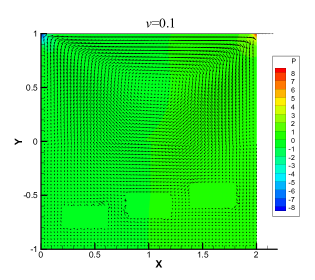
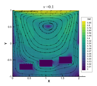
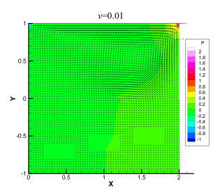
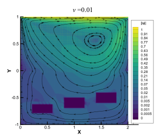
Figure 2: (Left) Numerical velocity and pressure under different initial conditions on a triangular mesh with h =$\frac{1}{16}$; (Right) The streamlines of velocity.

5.3 A 3D-example with closed form solution

Finally, we test our algorithms for solving a three-dimensional problem with closed form solution. Let $\Omega\subset\mathbb{R}^{3}$ with $\Omega_{f}=(0,1)\times(0,1)\times(0,1),\Omega_{p}=(0,1)\times(0,1)\times$ $(1,2)$ and the interface $\Gamma=(0,1)\times\{1\}$. The exact solution $(\bm{u},\varphi,p)$ is given by

$$\begin{cases}u=-(1-y)(1-z)&\text{ in }\Omega_{f},\\ v=-(1-x)(1-z)&\text{ in }\Omega_{f},\\ w=(1-x)(1-y)&\text{ in }\Omega_{f},\\ p=(1-z)(1-x-y-z+4xyz)&\text{ in }\Omega_{f},\\ \varphi=(1-x)(1-y)(1-z)&\text{ in }\Omega_{p},\end{cases}$$

where the components of $\bm{u}$ is denoted by $(u,v,w)$. All the parameters except $\nu$ in the coupled model are set to be 1. In (4.2), we set $\gamma_{1}=1,\gamma_{2}=1,B_{\bm{u}}({\bm{x}})=xyz(x-1)(y-1)$ and $B_{\varphi}(\bm{x})=xy(x-1)(y-1)(z-2)$. The uniform triangulation $\mathcal{T}_{h}$ with mesh size $h=\frac{1}{32}$ is adopted to be the test locations.

Similar to the 2D situation, we denote the components of $\bm{u}^{DL}$ obtained by Algorithm 1 as $(u^{DL},v^{DL},w^{DL})$ and test the computational performance of Algorithm 1 and Algorithm 2. From Table 13$-$ Table 14, we observe that the absolute discrete maximum errors of $u,v$, $w$, $p$ and $\varphi$ can reach $O(10^{-3})$ or $O(10^{-4})$. However, decreasing the iteration steps cannot further improve accuracy. In order to illustrate the accuracy of the Int-Deep method, we compare the iteration steps $\#\mathrm{K}$ of Newton iterative method employing different initial guesses with $h=\frac{1}{2^{k}}$, $k=2,3,4$. The corresponding results are presented in Tables 15 $-$ 16. As we can see, when the viscosity coefficient $\nu$ decreases, only the Int-Deep method can converge with few iteration steps.

$\#$Epoch	$||u-u^{DL}||_{0,\infty,h}$	$||v-v^{DL}||_{0,\infty,h}$	$||w-w^{DL}||_{0,\infty,h}$	$||p-p^{DL}||_{0,\infty,h}$	$||\varphi-\varphi^{DL}||_{0,\infty,h}$
200	1.1280e-01	1.1474e-01	1.2573e-01	9.8521e-01	1.9437e-01
500	5.8955e-03	6.0989e-03	4.6234e-03	1.8171e-01	7.3369e-03
1000	3.9364e-03	4.6433e-03	3.1881e-03	6.4626e-02	4.4960e-03
1500	8.2522e-03	8.5444e-03	8.1683e-03	2.9225e-02	2.2214e-03
2000	1.0683e-03	1.0316e-03	7.5461e-04	1.5038e-02	9.4810e-04
2500	2.4907e-03	2.4303e-03	2.6002e-03	1.2858e-02	8.1199e-04
2500	2.4907e-03	2.4303e-03	2.6002e-03	1.2858e-02	8.1199e-04
3000	7.7432e-04	1.1575e-03	1.1627e-03	8.1957e-03	1.2877e-03
3500	4.7258e-04	6.2618e-04	4.2063e-04	6.4445e-03	8.3823e-04
5000	3.6597e-04	6.0589e-04	3.5250e-04	7.9574e-03	6.8734e-04
7500	2.8277e-04	4.7100e-04	3.0724e-04	3.4871e-03	4.7562e-04
10000	1.3952e-04	3.0117e-04	2.9271e-04	3.3414e-03	3.3065e-04
15000	1.6717e-04	2.4263e-04	2.3134e-04	2.9260e-03	2.9287e-04
20000	1.3941e-04	2.2699e-04	2.1378e-04	2.5956e-03	2.9260e-04

Table 13: The absolute discrete maximum errors of Algorithm1 with $\nu=1,\kappa=1$.

$\#$Epoch	$||u-u^{DL}||_{0,\infty,h}$	$||v-v^{DL}||_{0,\infty,h}$	$||w-w^{DL}||_{0,\infty,h}$	$||p-p^{DL}||_{0,\infty,h}$	$||\varphi-\varphi^{DL}||_{0,\infty,h}$
200	4.9421e-02	3.9340e-02	1.1578e-01	3.6239e-02	4.6330e-02
500	2.6120e-02	1.6990e-02	3.8038e-02	8.8871e-03	1.4511e-02
1000	1.7341e-02	1.1687e-02	2.1754e-02	8.6221e-03	8.6668e-03
1500	1.3706e-02	7.0937e-03	1.6307e-02	2.8401e-03	4.4740e-03
2000	1.2608e-02	5.5066e-03	1.3255e-02	2.1570e-03	3.2142e-03
2500	9.4278e-03	5.1800e-03	1.1713e-02	2.0543e-03	2.5913e-03
2500	9.4278e-03	5.1800e-03	1.1713e-02	2.0543e-03	2.5913e-03
3000	8.6336e-03	3.9181e-03	9.9709e-03	2.0516e-03	2.3925e-03
3500	7.9073e-03	3.6801e-03	9.5410e-03	2.6332e-03	1.8229e-03
5000	5.8340e-03	3.3927e-03	7.2748e-03	7.1876e-04	1.3675e-03
7500	3.9786e-03	3.3174e-03	5.5008e-03	3.2889e-04	1.0128e-03
10000	3.3260e-03	2.7889e-03	4.4905e-03	2.9798e-04	8.3913e-04
15000	2.7782e-03	2.3925e-03	3.9075e-03	1.8952e-04	6.8426e-04
20000	2.6754e-03	2.3359e-03	3.8142e-03	2.1757e-04	7.0270e-04

Table 14: The absolute discrete maximum errors of Algorithm 1 with $\nu=0.01,\;\kappa=1$.

	$h=\frac{1}{4}$	$h=\frac{1}{8}$	$h=\frac{1}{16}$
$\bm{u}_{0}^{SD}$	4	4	4
$\bm{0}$	5	5	5
$\bm{1}$	5	5	5
$\bm{u}_{0}^{DL}$	4	4	4

Table 15: The number of iterations $\#$K under different initial values with $\nu=1,\;\kappa=1$.

	$h=\frac{1}{4}$	$h=\frac{1}{8}$	$h=\frac{1}{16}$
$\bm{u}^{SD}_{0}$	7	7	7
$\bm{0}$	8	8	8
$\bm{1}$	8	8	8
$\bm{u}^{DL}_{0}$	5	5	5

Table 16: The number of iterations $\#$K under different initial values with $\nu=0.01,\;\kappa=1$.

Table 18$-$Table 18 show that the orders of relative errors in $L^{2}$ norm for $\bm{u},p$ and $\varphi$ are $O(h^{3.7}),O(h^{2})$ and $O(h^{3}),$ respectively, and the orders of relative errors in $H^{1}$ norm for $\bm{u}$ and $\varphi$ are $O(h^{2.7})$ and $O(h^{2}),$ respectively, which is consistent with theoretical results.

	$\|\bm{e}_{\bm{u}}^{h}\|_{0}$	order	$\|e_{p}^{h}\|_{0}$	order	$\|e^{h}_{\varphi}\|_{0}$	order	$\|\bm{e}_{\bm{u}}^{h}\|_{1}$	order	$\|e^{h}_{\varphi}\|_{1}$	order
h$=\frac{1}{4}$	1.2611e-04	-	1.4169e-03	-	7.8653e-02	-	7.5859e-04	-	1.3749e-02	-
h$=\frac{1}{8}$	9.6019e-06	3.7152	1.9505e-02	2.0117	9.3657e-05	3.0179	2.2331e-04	2.6656	3.4647e-03	1.9886
h$=\frac{1}{16}$	7.2685e-07	3.7236	4.8542e-03	2.0065	1.1678e-05	3.0036	3.4100e-05	2.7112	8.6976e-04	1.9940

Table 17: The errors of Algorithm 2 with $\nu=1,\;\kappa=1$.

	$\|\bm{e}_{\bm{u}}^{h}\|_{0}$	order	$\|e_{p}^{h}\|_{0}$	order	$\|e^{h}_{\varphi}\|_{0}$	order	$\|\bm{e}_{\bm{u}}^{h}\|_{1}$	order	$\|e^{h}_{\varphi}\|_{1}$	order
h$=\frac{1}{4}$	1.1766e-02	-	7.8758e-02	-	7.9584e-04	-	1.3575e-01	-	1.3819e-02	-
h$=\frac{1}{8}$	8.8893e-04	3.7264	1.9508e-02	2.0134	9.4602e-05	3.0725	2.1471e-02	2.6605	3.4671e-03	1.9948
h$=\frac{1}{16}$	6.6064e-05	3.7501	4.8543e-03	2.0067	1.1691e-05	3.0165	3.2525e-03	2.7227	8.6985e-04	1.9949

Table 18: The errors of Algorithm 2 with $\nu=0.01,\;\kappa=1$.

6 Conclusion

In this paper, we develop a deep learning initialized iterative (Int-Deep) method for Navier-Stokes Darcy model. In this method, we employ the neural network solution generated by a few training steps as the initial guess for Newton iterative method with the FEM discretized problem. This hybrid method can converge to the true solution with the accuracy of FEM method rapidly. Numerical experiments also show that the method is robust when the model parameters vary over a large range.

References

• [1] R.A. Adams, Sobolev Spaces, Academic Press, New York, 1975.
• [2] T. Arbogast, D.S. Brunson, A computationalmethod for approximating a Darcy-Stokes system governing a vuggy porous medium, Comput. Geosci., 11 (2007), 207-218.
• [3] T. Arbogast, H.L. Lehr, Homogenization of a Darcy-Stokes system modeling vuggy porous media, Comput. Geosci., 10 (2006), 291-302.
• [4] L. Badea, M. Discacciati, A. Quarteroni, Mathematical Analysis of the Navier-Stokes and Darcy Coupling, Technical report, Politecnico di Milano, Milan, 2006.
• [5] L. Badea, M. Discacciati, A. Quarteroni, Numerical analysis of the Navier-Stokes Darcy coupling, Numer. Math., 115 (2010), 195-227.
• [6] J. Berg, K. Nyström, A unified deep artificial neural network approach to partial differential equations in complex geometries, Neurocomputing , 317 (2018), 28-41.
• [7] D. Boffi, F. Brezzi, M. Fortin, Mixed Finite Element Methods and Applications, Springer, Berlin, 2013.
• [8] S.C. Brenner, L.R. Scott, The Mathematical Theory of Finite Element Methods (Third Edition), Springer, New York, 2008.
• [9] M. Cai, M. Mu, J. Xu, Numerical solution to a mixed Navier-Stokes Darcy model by the two-grid approach, SIAM J. Numer. Anal., 47 (2009), 3325-3338.
• [10] Y. Cao, M. Gunzburger, X. Hu, F. Hua, X. Wang, W. Zhao, Finite element approximations for Stokes-Darcy flow with Beavers-Joseph interface conditions, SIAM J. Numer. Anal., 47 (2010), 4239-4256.
• [11] F. Chen, J. Huang, C. Wang, H. Yang, Friedrichs learning: weak solutions of partial differential equations via deep learning SIAM J. Sci. Comput., 45 (2023), 1271-1299.
• [12] J. Chen, X. Chi, W. E, Z. Yang, Bridging Traditional and Machine Learning-Based Algorithms for Solving PDEs: The Random Feature Method, J. Mach. Learn., 1 (2022), 268-298.
• [13] P. Chidyagwai, B. Riviére, On the solution of the coupled Navier-Stokes and Darcy equations, Comput. Methods Appl. Mech. Engrg., 198 (2009), 3806-3820.
• [14] P.G. Ciarlet, The Finite Element Method for Elliptic Problems, North-Holland, Amsterdam, 1978.
• [15] M. Discacciati, Domain Decomposition Methods for the Coupling of Surface and Groundwater Flows, Ph.D. thesis, Ecole Polytechnique Fédérale de Lausanne, Lausanne, Switzerland, 2004.
• [16] M. Discacctiati, E. Miglio, A. Quarteroni, Mathematical and numerical models for coupling surface and groundwater flows, Appl. Numer. Math., 43 (2002), 57-74.
• [17] M. Discacciati, A. Quarteroni, Navier-Stokes Darcy coupling: modeling, analysis, and numerical approximation, Rev. Mat. Complut., 22 (2009), 315-426.
• [18] S. Dong, Z. Li, Local extreme learning machines and domain decomposition for solving linear and nonlinear partial differential equations, Comput. Methods Appl. Mech. Engrg., 387 (2021), 114129.
• [19] G. Du, L. Zuo, Local and parallel partition of unity scheme for the mixed Navier-Stokes-Darcy problem, Numer. Algorithms, 91 (2022), 635-650.
• [20] W. E, Machine Learning and Computational Mathematics, Commun. Comput. Phys., 28 (2020), 1639-1670.
• [21] W. E, B. Yu, The Deep Ritz Method: A Deep Learning-Based Numerical Algorithm for Solving Variational Problems, Commun. Math. Stat., 6 (2018), 1-12.
• [22] V. Girault, B. Riviére, DG approximation of coupled Navier-Stokes and Darcy equations by Beaver-Joseph-Saffman interface condition, SIAM J. Numer. Anal., 47 (2009), 2052-2089.
• [23] I. Goodfellow, Y. Bengio, A. Courville, Deep Learning, MIT Press, 2016.
• [24] J. Han, A. Jentzen, W. E, Solving high-dimensional partial differential equations using deep learning, Proc. Natl. Acad. Sci. USA, 115 (2018), 8505-8510.
• [25] N. Hanspal, A. Waghode, V. Nassehi, R. Wakeman, Numerical analysis of coupled Stokes/Darcy flow in industrial filtrations, Transp. Porous Media., 64 (2006), 73-101.
• [26] G. Harper, J. Liu, S. Tavener, T. Wildey, Coupling Arbogast–Correa and Bernardi–Raugel elements to resolve coupled Stokes–Darcy flow problems, Comput. Methods Appl. Mech. Engrg., 373 (2021), 113469.
• [27] K. He, X. Zhang, S. Ren, J. Sun, Deep Residual Learning for Image Recognition, in: 2016 IEEE Conference on Computer Vision and Pattern Recognition (CVPR), 2016, 770-778.
• [28] Y. He, J. Li, Convergence of three iterative methods based on the finite element discretization for the stationary Navier-Stokes equations, Comput. Methods Appl. Mech. Engrg., 198 (2009), 1351-1359.
• [29] J. Huang, C. Wang, H. Wang, A Deep Learning Method for Elliptic Hemivariational Inequalities, East Asian J. Appl. Math., 12 (2022), 487-502.
• [30] J. Huang, H. Wang, H. Yang, Int-Deep: a deep learning initialized iterative method for nonlinear problems, J. Comput. Phys., 419 (2020), 109675.
• [31] T.J.R. Hughes, The Finite Element Method, Linear Static and Dynamic Finite Element Analysis, Prentice-Hall, Englewood Cliffs, N.J, 1987.
• [32] D.P. Kingma, J. Ba, Adam: A method for stochastic optimization, 2014, arXiv preprint arXiv:1412.6980.
• [33] W. Layton, H. Tran, C. Trenchea, Analysis of long time stability and errors of two partitioned methods for uncoupling evolutionary groundwater-surface water flows, SIAM J. Numer. Anal., 51 (2013), 248-272.
• [34] W. Li, M.Z. Bazant, J. Zhu, A physics-guided neural network framework for elastic plates: comparison of governing equations-based and energy-based approaches, Comput. Methods Appl. Mech. Engrg., 383 (2021), 113933.
• [35] L. Lu, X. Meng, Z. Mao, G. Karniadakis DeepXDE: A Deep Learning Library for Solving Differential Equations, SIAM Rev., 63 (2021), 208-228.
• [36] C. Qiu, X. He, J. Li, Y. Lin, A domain decomposition method for the time-dependent Navier-Stokes-Darcy model with Beavers-Joseph interface condition and defective boundary condition, J. Comput. Phys., 411 (2020), 109400.
• [37] M. Raissi, P. Perdikaris, G. Karniadakis, Physics-informed neural networks: A deep learning framework for solving forward and inverse problems involving nonlinear partial differential equations, J. Comput. Phys., 378 (2019), 686-707.
• [38] R. Temam, Navier-Stokes Equations, North-Holland, Amsterdam, 1979.
• [39] Z. Xu, Frequency principle: Fourier analysis sheds light on deep neural networks, Commun. Comput. Phys., 28 (2020), 1746-1767.
• [40] Z. Xu, Y. Zhang, Y. Xiao, Training behavior of deep neural network in frequency domain, In International Conference on Neural Information Processing, Springer, 2019, 264-274.
• [41] J. Yu, L. Lu, X. Meng, G. Karniadakis, Gradient-enhanced physics-informed neural networks for forward and inverse PDE problems, Comput. Methods Appl. Mech. Engrg., 393 (2022), 114823.
• [42] Y. Zang, G. Bao, X. Ye, H. Zhou, Weak adversarial networks for high-dimensional partial differential equations, J. Comput. Phys., 411 (2020), 109409.
• [43] L. Zuo, Y. Hou, Numerical analysis for the mixed Navier-Stokes and Darcy problem with the Beavers-Joseph interface condition, Numer. Methods Partial Differential Equations, 31 (2015), 1009-1030.