Symbol as Points: Panoptic Symbol Spotting via Point-based Representation

Abstract

This work studies the problem of panoptic symbol spotting, which is to spot and parse both countable object instances (windows, doors, tables, etc.) and uncountable stuff (wall, railing, etc.) from computer-aided design (CAD) drawings. Existing methods typically involve either rasterizing the vector graphics into images and using image-based methods for symbol spotting, or directly building graphs and using graph neural networks for symbol recognition. In this paper, we take a different approach, which treats graphic primitives as a set of 2D points that are locally connected and use point cloud segmentation methods to tackle it. Specifically, we utilize a point transformer to extract the primitive features and append a mask2former-like spotting head to predict the final output. To better use the local connection information of primitives and enhance their discriminability, we further propose the attention with connection module (ACM) and contrastive connection learning scheme (CCL). Finally, we propose a KNN interpolation mechanism for the mask attention module of the spotting head to better handle primitive mask downsampling, which is primitive-level in contrast to pixel-level for the image. Our approach, named SymPoint, is simple yet effective, outperforming recent state-of-the-art method GAT-CADNet by an absolute increase of 9.6% PQ and 10.4% RQ on the FloorPlanCAD dataset. The source code and models will be available at https://github.com/nicehuster/SymPoint.

1 Introduction

Vector graphics (VG), renowned for their ability to be scaled arbitrarily without succumbing to issues like blurring or aliasing of details, have become a staple in industrial designs. This includes their prevalent use in graphic designs(Reddy et al., 2021), 2D interfaces(Carlier et al., 2020), and Computer-aided design (CAD)(Fan et al., 2021). Specifically, CAD drawings, consisting of geometric primitives(e.g., arc, circle, polyline, etc.), have established themselves as the preferred data representation method in the realms of interior design, indoor construction, and property development, promoting a higher standard of precision and innovation in these fields.

Symbol spotting (Rezvanifar et al., 2019; 2020; Fan et al., 2021; 2022; Zheng et al., 2022) refers to spotting and recognizing symbols from CAD drawings, which serves as a foundational task for reviewing the error of design drawing and 3D building information modeling (BIM). Spotting each symbol, a grouping of graphical primitives, within a CAD drawing poses a significant challenge due to the existence of obstacles such as occlusion, clustering, variations in appearances, and a significant imbalance in the distribution of different categories. Traditional symbol spotting usually deals with instance symbols representing countable things (Rezvanifar et al., 2019), like table, sofa, and bed. Fan et al. (2021) further extend it to panoptic symbol spotting which performs both the spotting of countable instances (e.g., a single door, a window, a table, etc.) and the recognition of uncountable stuff (e.g., wall, railing, etc.).

Typical approaches (Fan et al., 2021; 2022) addressing the panoptic symbol spotting task involve first converting CAD drawings to raster graphics(RG) and then processing it with powerful image-based detection or segmentation methods (Ren et al., 2015; Sun et al., 2019). Another line of previous works (Jiang et al., 2021; Zheng et al., 2022; Yang et al., 2023) abandons the raster procedure and directly processes vector graphics for recognition with graph convolutions networks. Instead of rastering CAD drawings to images or modeling the graphical primitives with GCN/GAT, which can be computationally expensive, especially for large CAD graphs, we propose a new paradigm that has the potential to shed novel insight rather than merely delivering incremental advancements in performance.

Upon analyzing the data characteristics of CAD drawings, we can find that CAD drawing has three main properties: 1). irregularity and disorderliness. Unlike regular pixel arrays in raster graphics/images, CAD drawing consists of geometric primitives(e.g., arc, circle, polyline, etc.) without specific order. 2). local interaction among graphical primitives. Each graphical primitive is not isolated but locally connected with neighboring primitives, forming a symbol. 3). invariance under transformations. Each symbol is invariant to certain transformations. For example, rotating and translating symbols do not modify the symbol’s category. These properties are almost identical to point clouds. Hence, we treat CAD drawing as sets of points (graphical primitives) and utilize methodologies from point cloud analysis (Qi et al., 2017a; b; Zhao et al., 2021) for symbol spotting.

In this work, we first consider each graphic primitive as an 8-dimensional data point with the information of position and primitive’s properties (type, length, etc.). We then utilize methodologies from point cloud analysis for graphic primitive representation learning. Different from point clouds, these graphical primitives are locally connected. We therefore propose contrastive connectivity learning mechanism to utilize those local connections. Finally, we borrow the idea of Mask2Former(Cheng et al., 2021; 2022) and construct a masked-attention transformer decoder to perform the panoptic symbol spotting task. Besides, rather than using bilinear interpolation for mask attention downsampling as in (Cheng et al., 2022), which could cause information loss due to the sparsity of graphical primitives, we propose KNN interpolation, which fuses the nearest neighboring primitives, for mask attention downsampling. We conduct extensive experiments on the FloorPlanCAD dataset and our SymPoint achieves 83.3% PQ and 91.1% RQ under the panoptic symbol spotting setting, which outperforms the recent state-of-the-art method GAT-CADNet (Zheng et al., 2022) with a large margin.

2 Related Work

Vector Graphics Recognition

Vector graphics are widely used in 2D CAD designs, urban designs, graphic designs, and circuit designs, to facilitate resolution-free precision geometric modeling. Considering their wide applications and great importance, many works are devoted to recognition tasks on vector graphics.  Jiang et al. (2021) explores vectorized object detection and achieves a superior accuracy to detection methods (Bochkovskiy et al., 2020; Lin et al., 2017) working on raster graphics while enjoying faster inference time and less training parameters. Shi et al. (2022) propose a unified vector graphics recognition framework that leverages the merits of both vector graphics and raster graphics.

Panoptic Symbol Spotting

Traditional symbol spotting usually deals with instance symbols representing countable things (Rezvanifar et al., 2019), like table, sofa, and bed. Following the idea in (Kirillov et al., 2019), Fan et al. (2021) extended the definition by recognizing semantic of uncountable stuff, and named it panoptic symbol spotting. Therefore, all components in a CAD drawing are covered in one task altogether. For example, the wall represented by a group of parallel lines was properly handled by (Fan et al., 2021), which however was treated as background by  (Jiang et al., 2021; Shi et al., 2022; Nguyen et al., 2009) in Vector graphics recognition. Meanwhile, the first large-scale real-world FloorPlanCAD dataset in the form of vector graphics was published by (Fan et al., 2021). Fan et al. (2022) propose CADTransformer, which modifies existing vision transformer (ViT) backbones for the panoptic symbol spotting task. Zheng et al. (2022) propose GAT-CADNet, which formulates the instance symbol spotting task as a subgraph detection problem and solves it by predicting the adjacency matrix.

Point Cloud Segmentation

Point cloud segmentation aims to map the points into multiple homogeneous groups. Unlike 2D images, which are characterized by regularly arranged dense pixels, point clouds are constituted of unordered and irregular point sets. This makes the direct application of image processing methods to point cloud segmentation an impracticable approach. However, in recent years, the integration of neural networks has significantly enhanced the effectiveness of point cloud segmentation across a range of applications, including semantic segmentation (Qi et al., 2017a; a; Zhao et al., 2021), instance segmentation (Ngo et al., 2023; Schult et al., 2023) and panoptic segmentation (Zhou et al., 2021; Li et al., 2022; Hong et al., 2021; Xiao et al., 2023), etc.

3 Method

Our methods forgo the raster image or GCN in favor of a point-based representation for graphical primitives. Compared to image-based representations, it reduces the complexity of models due to the sparsity of primitive CAD drawings. In this section, we first describe how to form the point-based representation using the graphical primitives of CAD drawings. Then we illustrate a baseline framework for panoptic symbol spotting. Finally, we thoroughly explain three key techniques, attention with local connection, contrastive connection learning, and KNN interpolation, to adapt this baseline framework to better handle CAD data.

3.1 From Symbol to Points

Given vector graphics represented by a set of graphical primitives $\{\bm{p}_{k}\}$, we treat it as a collection of points $\{\bm{p}_{k}\mid(\bm{x}_{k},\bm{f}_{k})\}$, and each point contains both primitive position $\{\bm{x}_{k}\}$ and primitive feature $\{\bm{f}_{k}\}$ information; hence, the points set could be unordered and disorganized.

Primitive position. Given a graphical primitive, the coordinates of the starting point and the ending point are $(x_{1},y_{1})$ and $(x_{1},y_{2})$, respectively. The primitive position $\bm{x}_{k}\in\mathbb{R}^{2}$ is defined as :

$$\bm{x}_{k}=\left[(x_{1}+x_{2})/2,(y_{1}+y_{2})/2\right],$$ (1)

We take its center as the primitive position for a closed graphical primitive(circle, ellipse). as shown in Fig. 1(a).

Primitive feature. We define the primitive features ${f}_{k}\in\mathbb{R}^{6}$ as:

$$\bm{f}_{k}=\left[\alpha_{k},l_{k},onehot(t_{k})\right],$$ (2)

where $\alpha_{k}$ is the clockwise angle from the $x$ positive axis to $x_{k}$, and $l_{k}$ measures the length of $v_{1}$ to $v_{2}$, as shown in Fig. 1(b). We encode the primitive type $t_{k}$(line, arc, circle, or ellipse) into a one-hot vector to make up the missing information of segment approximations.

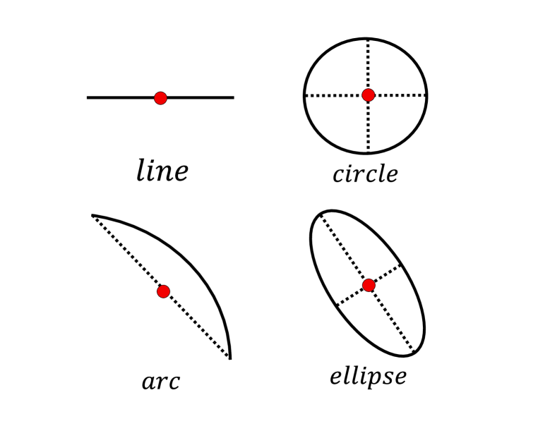
((a)) primitive position.

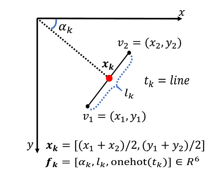
((b)) primitive feature.

Figure 1: Illustration of constructing point-based representation.

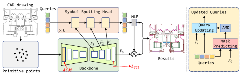
Figure 2: The overview of our method. After transfering CAD drawings to primitive points, we use a backbone to extract multi-resolution features $F_{r}$ and append a symbol spotting head to spot and recognize symbols. During this process, we propose attention with connection module(ACM), which utilizes primitive connection information when performing self-attention in the first stage of backone. Subsequently, we propose contrastive connection learning(CCL) to enhance the discriminability between connected primitive features. Finally, we propose KNN interpolation for attention mask downsampling(AMD) to effetively downsample the high-resolution attention masks.

3.2 Panoptic Symbol Spotting via Point-based Representation

The baseline framework primarily comprises two components: the backbone and the symbol spotting head. The backbone converts raw points into points features, while the symbol spotting head predicts the symbol mask through learnable queries (Cheng et al., 2021; 2022). Fig. 2 illustrates the the whole framework.

Backbone.

We choose Point Transformer (Zhao et al., 2021) with a symmetrical encoder and decoder as our backbone for feature extraction due to its good generalization capability in panoptic symbol spotting. The backbone takes primitive points as input, and performs vector attention between each point and its adjacent points to explore local relationships. Given a point ${\bm{p}}_{i}$ and its adjacent points $\mathcal{M}({\bm{p}}_{i})$, we project them into query feature ${\bm{q}}_{i}$, key feature ${\bm{k}}_{j}$ and value feature ${\bm{v}}_{j}$, and obtain the vector attention as follows:

$${\bm{w}}_{ij}=\omega(\gamma({\bm{q}}_{i},{\bm{k}}_{j})),\qquad f_{i}^{\text{attn}}=\sum_{{\bm{p}}_{j}\in\mathcal{M}({\bm{p}}_{i})}\text{Softmax}({\bm{W}}_{i})_{j}\odot{\bm{v}}_{j},$$ (3)

where $\gamma$ serves as a relational function, such as subtraction. $\omega$ is a learnable weight encoding that calculates the attention vectors. $\odot$ is Hadamard product.

Symbol Spotting Head.

We follow Mask2Former (Cheng et al., 2022) to use hierarchical multi-resolution primitive features $F_{r}\in{\mathbb{R}}^{N_{r}\times D}$ from the decoder of backbone as the input to the symbol spotting predition head, where $N_{r}$ is the number of feature tokens in resolution $r$ and $D$ is the feature dimension. This head consists of $L$ layers of masked attention modules which progressively upscales low-resolution features from the backbone to produce high-resolution per-pixel embeddings for mask prediction. There are two key components in the masked attention module: query updating and mask predicting. For each layer $l$, query updating involves interacting with different resolution primitive features $F_{r}$ to update query features. This process can be formulated as,

$$X_{l}=\mathrm{softmax}(A_{l-1}+Q_{l}K_{l}^{T})V_{l}+X_{l-1},$$ (4)

where $X_{l}\in{\mathbb{R}}^{O\times D}$ is the query features. $O$ is the number of query features. $Q_{l}=f_{Q}(X_{l-1})$, $K_{l}=f_{K}(F_{r})$ and $V_{l}=f_{V}(F_{r})$ are query, key and value features projected by MLP layers. $A_{l-1}$ is the attention mask, which is computed by,

$$A_{l-1}(v)=\left\{\begin{array}[]{rcl}0&&\text{if}\ M_{l-1}(v)>0.5,\\ -\infty&&\text{otherwise}.\end{array}\right.$$ (5)

where $v$ is the position of feature point and $M_{l-1}$ is the mask predicted from mask predicting part. Note that we need to downsample the high-resolution attention mask to adopt the query updating on low-resolution features. In practice, we utilize four coarse-level primitive features from the decoder of backbone and perform query updating from coarse to fine.

During mask predicting process, we obtain the object mask $M_{l}\in{\mathbb{R}}^{O\times N_{0}}$ and its corresponding category $Y_{l}\in{\mathbb{R}}^{O\times C}$ by projecting the query features using two MLP layers $f_{Y}$ and $f_{M}$, where $C$ is the category number and $N_{0}$ is the number of points. The process is as follows:

$$Y_{l}=f_{Y}(X_{l}),\quad M_{l}=f_{M}(X_{l})F_{0}^{T},$$ (6)

The outputs of final layer, $Y_{L}$ and $M_{L}$, are the predicted results.

3.3 Attention with Connection Module

The simple and unified framework rewards excellent generalization ability by offering a fresh perspective of CAD drawing, a set of points. It can obtain competitive results compared to previous methods. However, it ignores the widespread presence of primitive connections in CAD drawings. It is precisely because of these connections that scattered, unrelated graphical elements come together to form symbols with special semantics. In order to utilize these connections between each primitive, we propose Attention with Connection Module (ACM), the details are shown below.

It is considered that these two graphical primitives($p_{i},p_{j}$) are interconnected if the minimum distance $d_{ij}$ between the endpoints $({\bm{v}}_{i},{\bm{v}}_{j})$ of two graphical primitives $({\bm{p}}_{i},{\bm{p}}_{j})$ is below a certain threshold $\epsilon$, where:

$$d_{ij}=\text{min}_{\bm{v}_{i}\in{\bm{p}}_{i},\bm{v}_{j}\in{\bm{p}}_{j}}\|\bm{v}_{i}-\bm{v}_{j}\|<\epsilon.$$ (7)

To keep the complexity low, at most $K$ connections are allowed for every graphical primitive by random dropping. Fig. 3(a) demonstrates the connection construction around the wall symbol, the gray line is the connection between two primitives. In practice, we set $\epsilon$ to 1.0px.

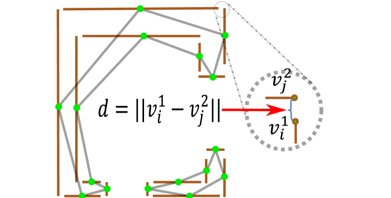
((a)) Construct connections.

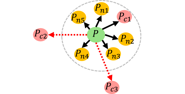
((b)) Attend to connections.

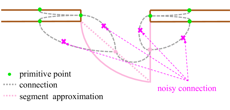
((c)) Noisy connections.

Figure 3: (a) Set of primitives and its connection, primitives are disintegrated for clarity. (b) Locally connected primitives are considered in the attention layers. (c) Locally connected primitives do not always belong to the same category.

The attention mechanism in (Zhao et al., 2021) directly performs local attention between each point and its adjacent points to explore the relationship. The original attention mechanism interacts only with neighboring points within a spherical region, as shown in Fig. 3(b). Our ACM additionally introduces the interaction with locally connected primitive points during attention (pink points), essentially enlarging the radius of the spherical region. Note that we experimentally found that crudely increasing the radius of the spherical region without considering the local connections of primitive points does not result in performance improvement. This may be explained by that enlarging the receptive field also introduces additional noise at the same time. Specifically, we extend the adjacent points set $\mathcal{M}({\bm{p}}_{i})$ in Eq. 3 to $\mathcal{A}({\bm{p}}_{i})=\mathcal{M}({\bm{p}}_{i})\cup\mathcal{C}({\bm{p}}_{i})$, where $\mathcal{C}({\bm{p}}_{i})=\{{\bm{p}}_{j}|d_{ij}<\epsilon\}$, yielding,

$$f_{i}^{\text{attn}}=\sum_{{\bm{p}}_{j}\in\mathcal{A}({\bm{p}}_{i})}\text{Softmax}({\bm{W}}_{i})_{j}\odot{\bm{v}}_{j},$$ (8)

In practice, since we cannot directly obtain the connection relationships of the points in the intermediate layers of the backbone, we integrate this module into the first stage of the backbone to replace the original local attention, as shown in Fig. 2.

3.4 Contrastive Connection Learning.

Although the information of primitive connection are considered when calculating attention of the encoder transformer, locally connected primitives may not belong to the same instance, in other words, noisy connections could be introduced while take primitive connections into consideration, as shown in Fig. 3(c). Therefore, in order to more effectively utilize connection information with category consistency, we follow the widely used InfoNCE loss (Oord et al., 2018) and its generalization (Frosst et al., 2019; Gutmann & Hyvärinen, 2010) to define the contrastive learning objective on the final output feature of backbone. We encourage learned representations more similar to its connected points from the same category and more distinguished from other connected points from different categories. Additionally, we also take neighbor points $\mathcal{M}({\bm{p}}_{i})$ into consideration, yielding,

$$L_{CCL}=-\log\frac{\sum_{{\bm{p}}_{j}\in{\mathcal{A}({\bm{p}}_{i})}\land l_{j}=l_{i}}\exp(-d({\bm{f}}_{i},{\bm{f}}_{j})/\tau)}{\sum_{{\bm{p}}_{k}\in{\mathcal{A}({\bm{p}}_{i})}}\exp(-d({\bm{f}}_{i},{\bm{f}}_{k})/\tau)}$$ (9)

where ${{\bm{f}}_{i}}$ is the backbone feature of ${\bm{p}}_{i}$, $d(\cdot,\cdot)$ is a distance measurement, $\tau$ is the temperature in contrastive learning. we set the $\tau$ = 1 by default.

3.5 KNN Interpolation

During the process of query updating in symbol spotting head Eq. 4 & Eq. 5, we need to convert high-resolution mask predictions to low-resolution for attention masks computation as shown in Fig. 2 (AMD on the right). Mask2Former (Cheng et al., 2022) employs the bilinear interpolation on the pixel-level mask for downsampling. However, the masks of CAD drawings are primitive-level, making it infeasible to directly apply the bilinear interpolation on them. To this end, we propose the KNN interpolation for downsampling the attention masks by fusing the nearest neighbor points. A straightforward operation is max pooling or average pooling. We instead utilize distance-based interpolation. For simplicity, we omit layer index $l$ in $A$,

$$A^{r}({\bm{p}}_{j})=\frac{\sum_{{\bm{p}}_{j}\in\mathcal{K}({\bm{p}}_{i})}A^{0}({{\bm{p}}_{j}})/d({\bm{p}}_{i},{\bm{p}}_{j})}{\sum_{{\bm{p}}_{j}\in\mathcal{K}({\bm{p}}_{i})}1/d({\bm{p}}_{i},{\bm{p}}_{j})}$$ (10)

where, $A^{0}$ and $A^{r}$ are the full-resolution attention mask and the $r$-resolution attention mask repectively. $d(\cdot,\cdot)$ is a distance measurement. $\mathcal{K}({\bm{p}}_{i})$ is the set of $K$ nearest neighbors, In practice, we set $K=4^{r}$ in our experiments.

3.6 Training and Inference

Throughout the training phase, we adopt bipartite matching and set prediction loss to assign ground truth to predictions with the smallest matching cost. The full loss function $L$ can be formulated as $L=\lambda_{BCE}L_{BCE}+\lambda_{dice}L_{dice}+\lambda_{cls}L_{cls}+\lambda_{CCL}L_{CCL}$, while $L_{BCE}$ is the binary cross-entropy loss (over the foreground and background of that mask), $L_{dice}$ is the Dice loss (Deng et al., 2018), $L_{cls}$ is the default multi-class cross-entropy loss to supervise the queries classification, $L_{CCL}$ is contrastive connection loss. In our experiments, we empirically set $\lambda_{BCE}:\lambda_{dice}:\lambda_{cls}:\lambda_{CCL}=5:5:2:8$. For inference, we simply use argmax to determine the final panoptic results.

4 Experiments

In this section, we present the experimental setting and benchmark results on the public CAD drawing dataset FloorPlanCAD (Fan et al., 2021). Following previous works (Fan et al., 2021; Zheng et al., 2022; Fan et al., 2022), we also compare our method with typical image-based instance detection (Ren et al., 2015; Redmon & Farhadi, 2018; Tian et al., 2019; Zhang et al., 2022). Besides, we also compare with point cloud semantic segmentation methods (Zhao et al., 2021), Extensive ablation studies are conducted to validate the effectiveness of the proposed techniques. In addition, we have also validated the generalizability of our method on other datasets beyond floorplanCAD, with detailed results available in the Appendix A.

4.1 Experimental Setting

Dataset and Metrics.

FloorPlanCAD dataset has 11,602 CAD drawings of various floor plans with segment-grained panoptic annotation and covering 30 things and 5 stuff classes. Following (Fan et al., 2021; Zheng et al., 2022; Fan et al., 2022), we use the panoptic quality (PQ) defined on vector graphics as our main metric to evaluate the performance of panoptic symbol spotting. By denoting a graphical entity $e=(l,z)$ with a semantic label $l$ and an instance index $z$, PQ is defined as the multiplication of segmentation quality (SQ) and recognition quality (RQ), which is formulated as

$$PQ =RQ\times SQ$$ (11)

$$=\frac{|TP|}{|TP|+\frac{1}{2}|FP|+\frac{1}{2}|FN|}\times\frac{\sum_{(s_{p},s_{g})\in TP}\text{IoU}(s_{p},s_{g})}{|TP|}$$ (12)

$$=\frac{\sum_{(s_{p},s_{g})\in TP}\text{IoU}(s_{p},s_{g})}{|TP|+\frac{1}{2}|FP|+\frac{1}{2}|FN|}.$$ (13)

where, $s_{p}=(l_{p},z_{p})$ is the predicted symbol, $s_{g}=(l_{g},z_{g})$ is the ground truth symbol. $|TP|$, $|FP|$, $|FN|$ indicate true positive, false positive and false negative respectively. A certain predicted symbol is considered as matched if it finds a ground truth symbol, with $l_{p}=l_{g}$ and IoU$(s_{p},s_{g})>0.5$, where the IoU is computed by:

$$\text{IoU}(s_{p},s_{g})=\frac{\Sigma_{e_{i}\in s_{p}\cap s_{g}}log(1+L(e_{i}))}{\Sigma_{e_{j}\in s_{p}\cup s_{g}}log(1+L(e_{j}))}.$$ (14)

Implementation Details.

We implement SymPoint with Pytorch. We use PointT (Zhao et al., 2021) with double channels as the backbone and stack $L=3$ layers for the symbol spotting head. For data augmentation, we adopt rotation, flip, scale, shift, and cutmix augmentation. We choose AdamW (Loshchilov & Hutter, 2017) as the optimizer with a default weight decay of 0.001, the initial learning rate is 0.0001, and we train the model for 1000 epochs with a batch size of 2 per GPU on 8 NVIDIA A100 GPUs.

4.2 Benchmark Results

Semantic symbol spotting.

We compare our methods with point cloud segmentation methods (Zhao et al., 2021), and symbol spotting methods (Fan et al., 2021; 2022; Zheng et al., 2022). The main test results are summarized in Tab. 1, Our algorithm surpasses all previous methods in the task of semantic symbol spotting. More importantly, compared to GAT-CADNet (Zheng et al., 2022), we achieves an absolute improvement of 1.8% F1. and 3.2% wF1 respectively. For the PointT^‡, we use our proposed point-based representation in Section 3.1 to convert the CAD drawing to a collection of points as input. It is worth noting that PointT^‡ has already achieved comparable results to GAT-CADNet (Zheng et al., 2022), which demonstrates the effectiveness of the proposed point-based representation for CAD symbol spotting.

Methods	PanCADNet	CADTransformer	GAT-CADNet	PointT‡	SymPoint
	(Fan et al., 2021)	(Fan et al., 2022)	(Zheng et al., 2022)	(Zhao et al., 2021)	(ours)
F1	80.6	82.2	85.0	83.2	86.8
wF1	79.8	80.1	82.3	80.7	85.5

Table 1: Semantic Symbol Spotting comparison results with previous works. $\ddagger$: backbone with double channels. wF1: length-weighted F1.

Method	Backbone	AP50	AP75	mAP	#Params	Speed
FasterRCNN (Ren et al., 2015)	R101	60.2	51.0	45.2	61M	59ms
YOLOv3 (Redmon & Farhadi, 2018)	DarkNet53	63.9	45.2	41.3	62M	11ms
FCOS (Tian et al., 2019)	R101	62.4	49.1	45.3	51M	57ms
DINO (Zhang et al., 2022)	R50	64.0	54.9	47.5	47M	42ms
SymPoint (ours)	PointT‡	66.3	55.7	52.8	35M	66ms

Table 2: Instance Symbol Spotting comparison results with image-based detection methods.

Method	Data Format	PQ	SQ	RQ	#Params	Speed
PanCADNet (Fan et al., 2021)	VG + RG	55.3	83.8	66.0	>42M	>1.2s
CADTransformer (Fan et al., 2022)	VG + RG	68.9	88.3	73.3	>65M	>1.2s
GAT-CADNet (Zheng et al., 2022)	VG	73.7	91.4	80.7	-	-
PointT‡Cluster(Zhao et al., 2021)	VG	49.8	85.6	58.2	31M	80ms
SymPoint(ours, 300epoch)	VG	79.6	89.4	89.0	35M	66ms
SymPoint(ours, 500epoch)	VG	81.9	90.6	90.4	35M	66ms
SymPoint(ours, 1000epoch)	VG	83.3	91.4	91.1	35M	66ms

Table 3: Panoptic Symbol Spotting comparisons results with previous works. VG: vector graphics, RG: raster graphics.

Instance Symbol Spotting.

We compare our method with various image detection methods, including FasterRCNN (Ren et al., 2015), YOLOv3 (Redmon & Farhadi, 2018), FCOS (Tian et al., 2019), and recent DINO (Zhang et al., 2022). For a fair comparison, we post-process the predicted mask to produce a bounding box for metric computation. The main comparison results are listed in Tab. 2. Although our framework is not trained to output a bounding box, it still achieves the best results.

Panoptic Symbol Spotting.

To verify the effectiveness of the symbol spotting head, we also design a variant method without this head, named PointT^‡Cluster, which predicts an offset vector per graphic entity to gather the instance entities around a common instance centroid and performs class-wise clustering (e.g. meanshift (Cheng, 1995)) to get instance labels as in CADTransformer (Fan et al., 2022). The final results are listed in Tab. 3. Our SymPoint trained with 300epoch outperforms both PointT^‡Cluster and the recent SOTA method GAT-CADNet(Zheng et al., 2022) substantially, demonstrate the effectiveness of the proposed method. Our method also benefits from longer training and achieves further performance improvement. What’s more, our method runs much faster during the inference phase than previous methods. For image-based methods, it takes approximately 1.2s to render a vector graphic into an image while our method does not need this process. The qualitative results are shown in Fig. 4(a).

4.3 Ablation Studies

In this section, we carry out a series of comprehensive ablation studies to clearly illustrate the potency and intricate details of the SymPoint framework. All ablations are conducted under 300 epoch training.

Baseline	ACM	CCL	KInter	PQ	RQ	SQ
✓				73.1	83.3	87.7
✓	✓			72.6	82.9	87.6
✓		✓		73.5	83.9	87.6
✓	✓	✓		74.3	85.8	86.6
✓	✓	✓	✓	77.3	87.1	88.7

((a)) Ablation studies of different techniques

DSampling method	PQ	RQ	SQ
linear	74.3	85.8	86.6
knn avepool	75.9	85.9	88.4
knn maxpool	77.0	86.7	88.8
knn interp	77.3	87.1	88.7

((b)) Ablation studies of mask downsampling

	BS	SW	$\mathrm{L}$	$\mathrm{O}$	$\mathrm{D}$	PQ	RQ	SQ	IoU	#Params
	1x	✓	3	300	128	67.1	78.7	85.2	62.8	9M
	1.5x	✓	3	300	128	73.3	84.0	87.3	65.6	19M
ablation setting	2x	✓	3	300	128	77.3	87.1	88.7	68.3	32M
	2x	✓	3	500	128	77.9	87.6	88.9	68.8	32M
final setting	2x	✓	3	500	256	79.6	89.0	89.4	69.1	35M
	2x		3	500	256	79.1	88.4	89.5	68.8	42M
	2x	✓	6	500	256	79.0	88.1	89.6	68.5	35M

((c)) Ablation studies on architecture design. BS: Backbone size. SW: share weights. $L$: layer number of spotting head. $O$: query number. $D$: feature dimension. $\checkmark$ in the share weights column means whether share weights for head layers.

Table 4: Ablation Stuides on different techniques, attention mask downsampling, and architecture desgin.

Effects of Techniques.

We conduct various controlled experiments to verify different techniques that improve the performance of SymPoint in Tab. 4(a). Here the baseline means the method described in Sec. 3.2. When we only introduce ACM (Attention with Connection Module), the performance drops a bit due to the noisy connections. But when we combine it with CCL (Contrastive Connection Learning), the performance improves to 74.3 of PQ. Note that applying CCL alone could only improve the performance marginally. Furthermore, KNN Interpolation boosts the performance significantly, reaching 77.3 of PQ.

KNN Interpolation.

In Tab. 4(b), we ablate different ways of downsampling attention mask: 1) linear interpolation, 2) KNN average pooling, 3) KNN max pooling, 4) KNN interpolation. KNN average pooling and KNN max pooling means using the averaged value or max value of the K nearest neighboring points as output instead of the one defined in Eq. 10. We can see that the proposed KNN interpolation achieves the best performance.

Architecture Design.

We analyze the effect of varying model architecture design, like channel number of backbone and whether share weights for the L layers of symbol spotting head. As shown in Tab. 4(c), we can see that enlarging the backbone, the query number and the feature channels of the symbol spotting head could further improve the performance. Sharing weights for spotting head not only saves model parameters but also achieves better performance compared with the one that does not share weights.

   

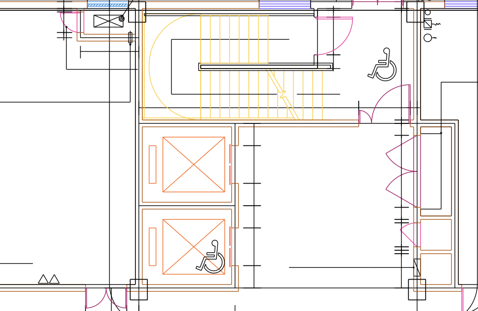
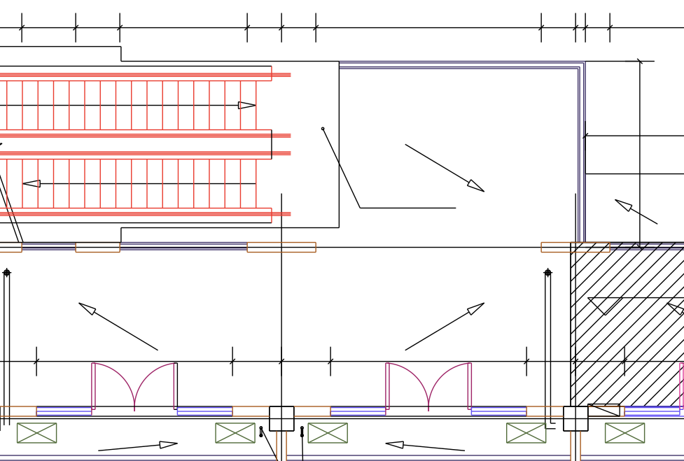
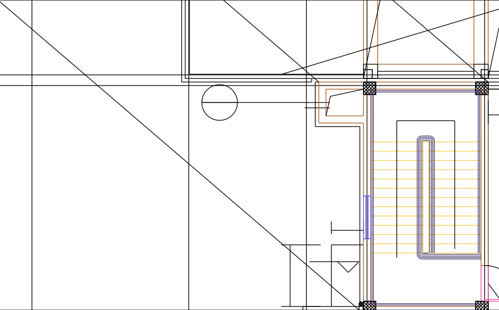
((a)) GT

   

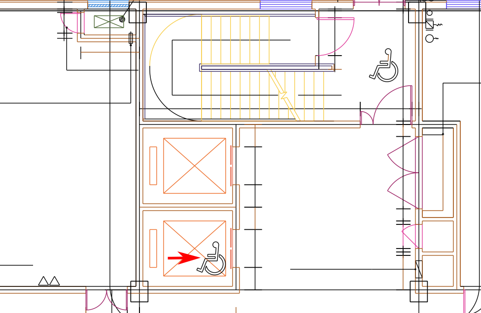
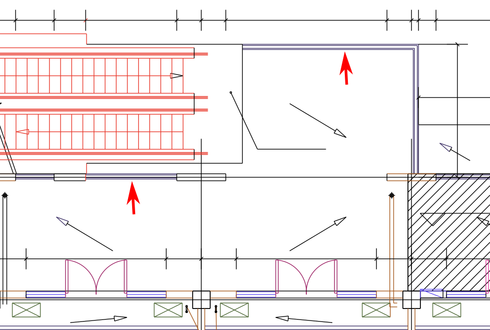
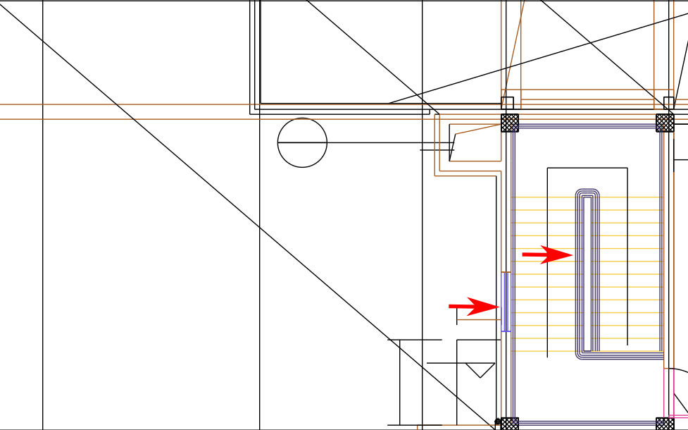
((b)) SymPoint

   

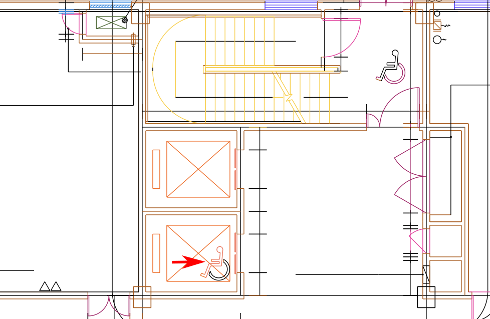
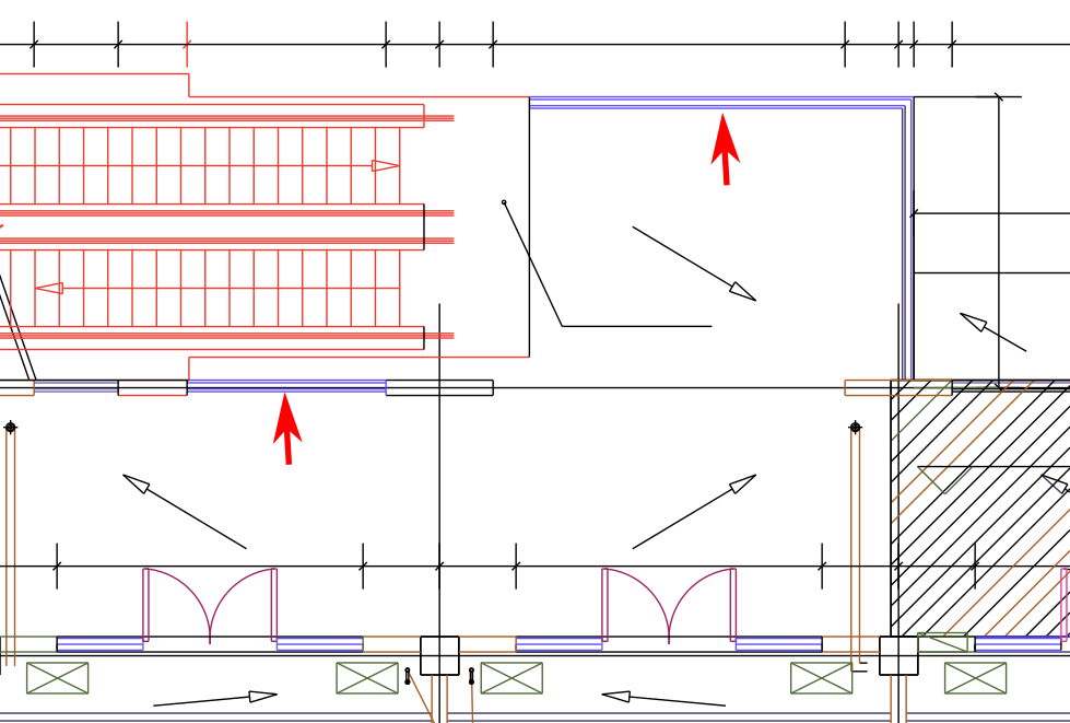
((c)) CADTransformer

Figure 4: Qualitative comparison of panoptic symbol spotting results with CADTransformer. Primitives belonging to different classes are represented in distinct colors. The colormap for each category can be referenced in Fig. 8.

   

5 Conclusion and Future Work

This work introduces a novel perspective for panoptic symbol spotting. We treat CAD drawings as sets of points and utilize methodologies from point cloud analysis for symbol spotting. Our method SymPoint is simple yet effective and outperforms previous works. One limitation is that our method needs a long training epoch to get promising performance. Thus accelerating model convergence is an important direction for future work.

Appendix A Appendix

Due to space constraints in the paper,additional techniques analysis, additional quantitative results, qualitative results, and other dataset results can be found in the supplementary materials.

A.1 Additional Techniques Analysis

Effects of Attention with Connection Module.

We conduct additional experiments in SESYD-floorplans dataset that is smaller than floorplanCAD. ACM can significantly promote performance and accelerate model convergence. We present the convergence curves without/with ACM in Fig. 5.

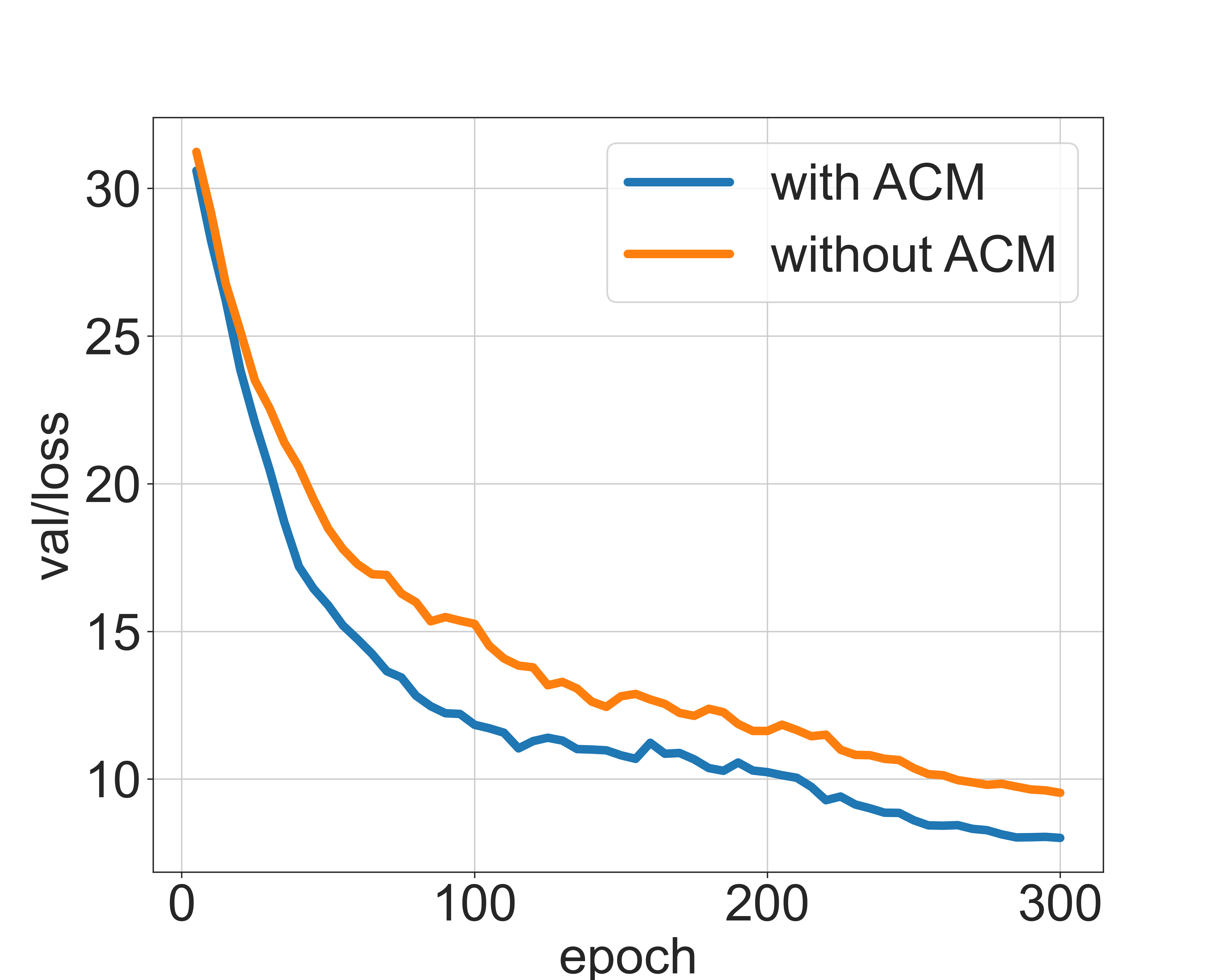
((a)) Loss curve.

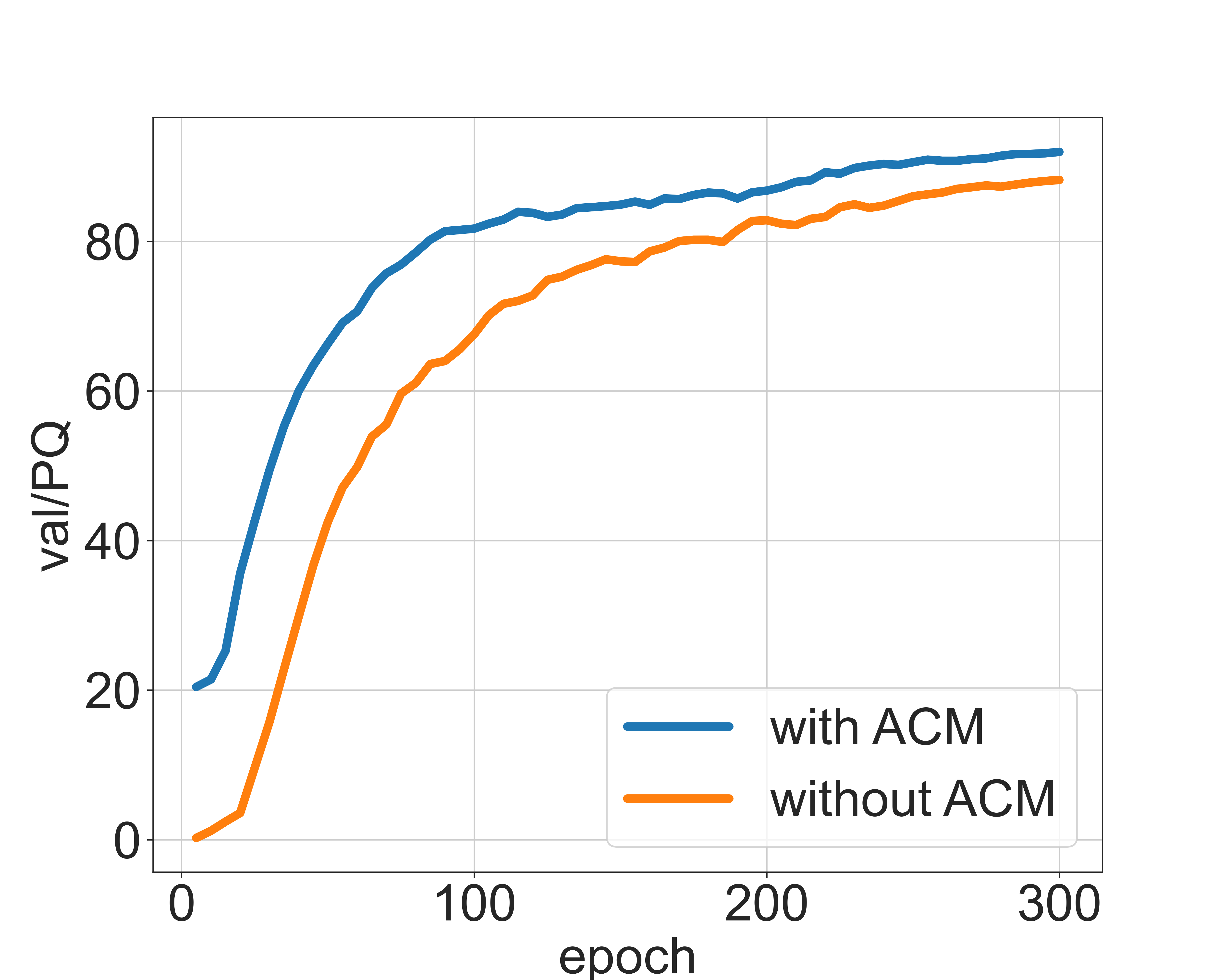
((b)) PQ curve.

Figure 5: Convergence curves with/without the ACM Module on SESYD-floorplans.

Explanation and Visualization of KNN interpolation Technique.

While bilinear interpolation, as utilized in Mask2Former, is tailored for regular data, such as image, but it is unsuitable for irregular sparse primitive points. Here, we provided some visualizations of point masks for KNN interpolation and bilinear interpolation as shown in Fig. 6(c). Note that these point masks are soft masks (ranging from 0 to 1) predicted by intermediate layers. After downsampling the point mask to 4x and 16x, we can clearly find that KNN interpolation well preserves the original mask information, while bilinear interpolation causes a significant information loss, which could harm the final performance.

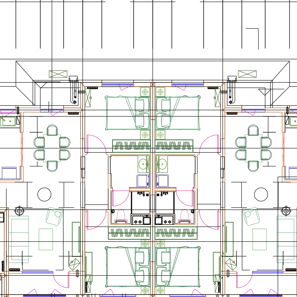
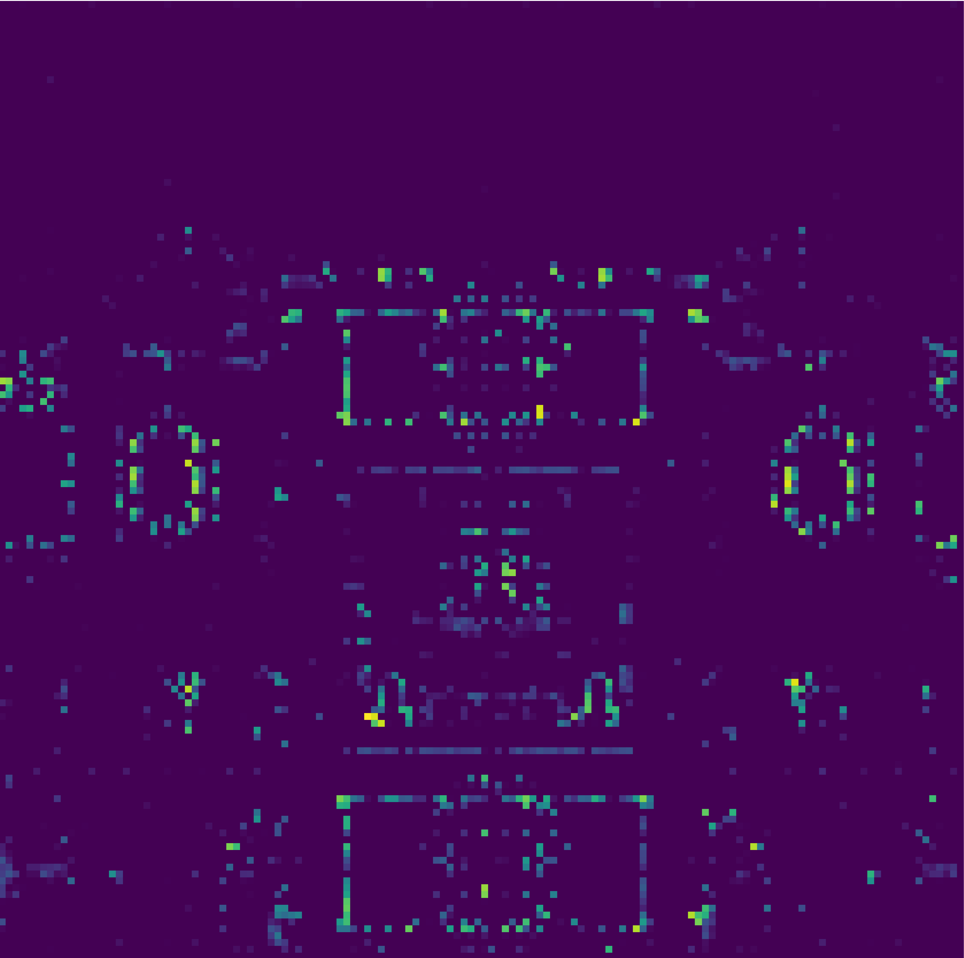
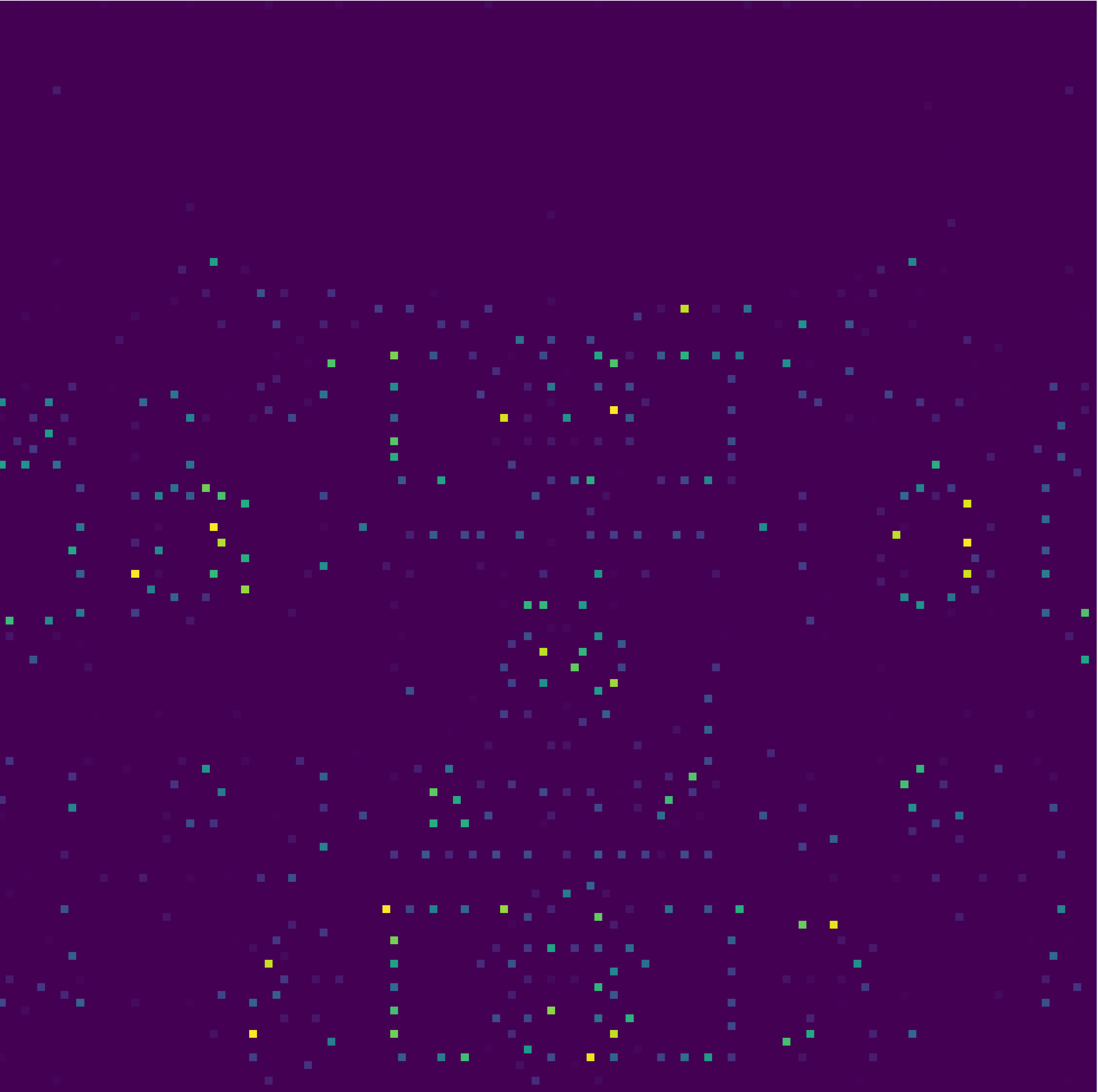
((a)) prediction

   

((b)) bilinear interp (down 4x)

((c)) bilinear interp (down 16x)

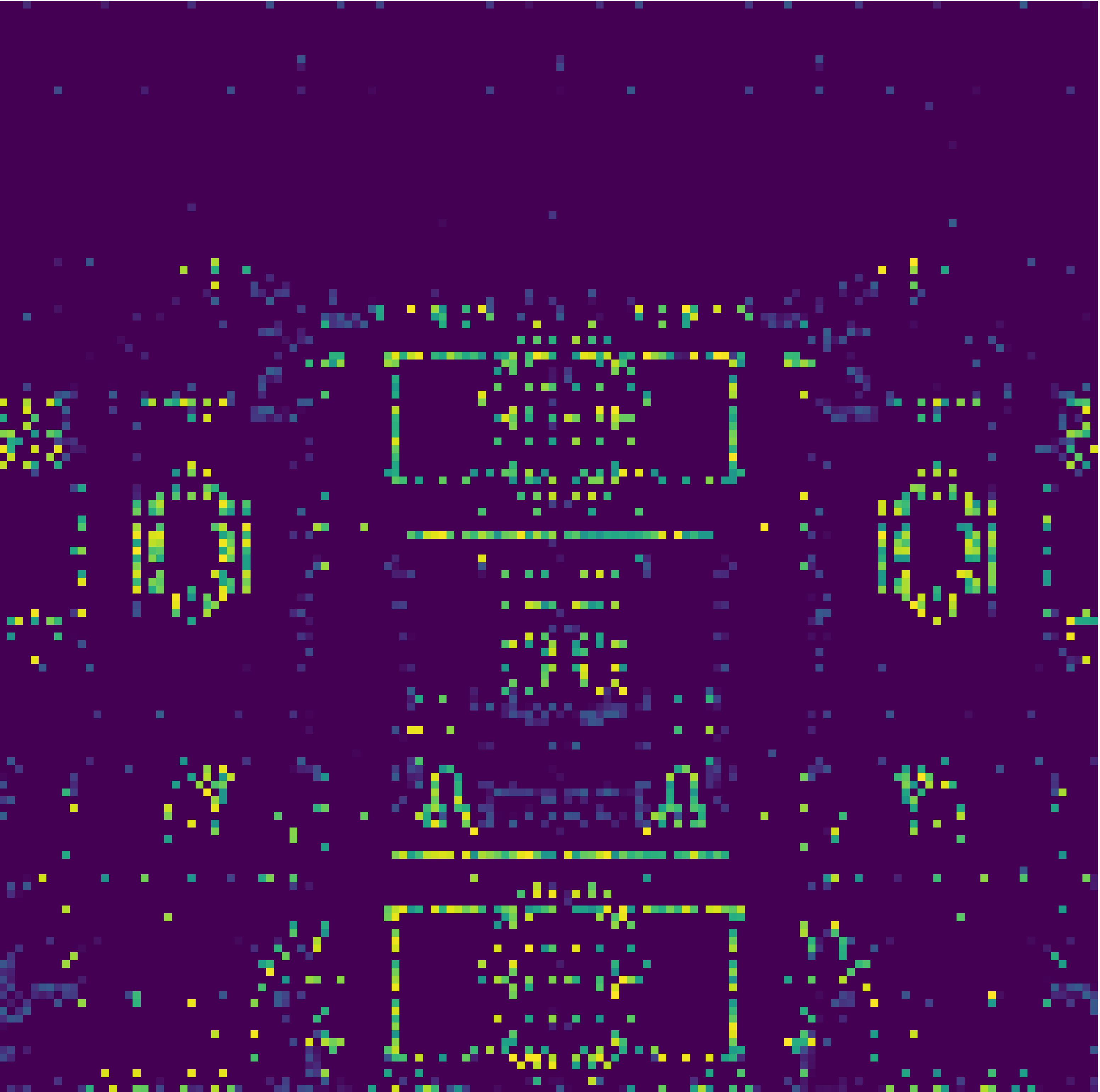
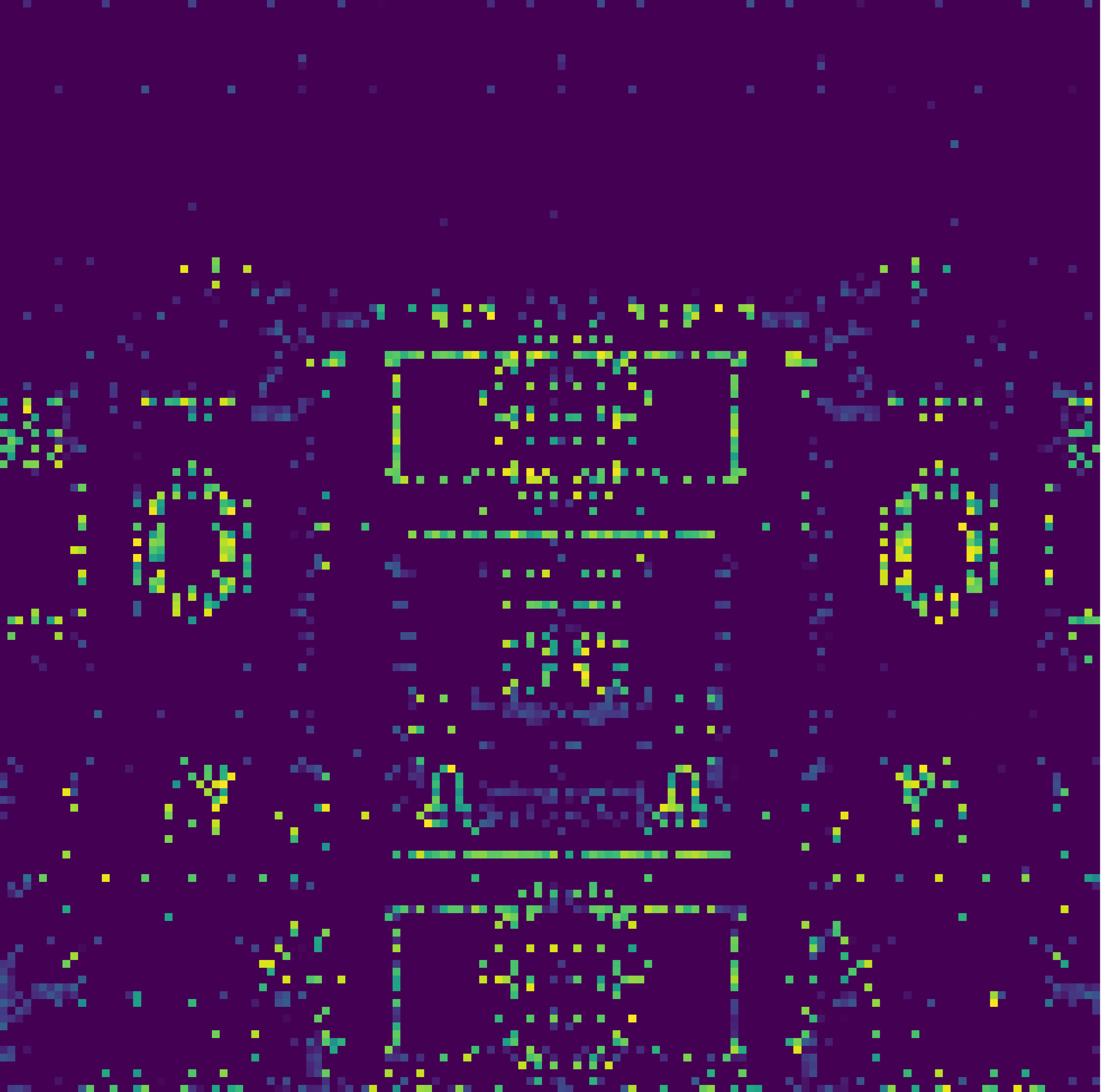
((d)) original point mask

   

((e)) KNN interp (down 4x)

((f)) KNN interp (down 16x)

Figure 6: KNN interp vs bilinear interp.

 

A.2 Additional Quantitative Evaluations

We present a detailed evaluation of panoptic quality(PQ), segmentation quality(SQ), and recognition quality(RQ) in Tab. 5. Here, we provide the class-wise evaluations of different variants of our methods.

Class	A			B			C			D			E
	PQ	RQ	SQ	PQ	RQ	SQ	PQ	RQ	SQ	PQ	RQ	SQ	PQ	RQ	SQ
single door	83.2	90.8	91.6	82.9	90.7	91.4	83.3	90.9	91.6	86.6	93.0	93.1	91.7	96.0	95.5
double door	86.8	93.8	92.5	85.8	93.4	91.9	86.5	93.5	92.5	88.5	95.3	92.9	91.5	96.6	94.7
sliding door	87.5	94.0	93.1	87.6	94.6	92.5	88.6	94.4	93.8	90.4	96.4	93.7	94.8	97.7	97.0
folding door	39.3	46.8	84.0	48.5	58.2	83.3	44.7	55.2	80.9	56.4	61.5	91.6	73.8	87.0	84.8
revolving door	0.0	0.0	0.0	0.0	0.0	0.0	0.0	0.0	0.0	0.0	0.0	0.0	0.0	0.0	0.0
rolling door	0.0	0.0	0.0	0.0	0.0	0.0	0.0	0.0	0.0	0.0	0.0	0.0	0.0	0.0	0.0
window	64.5	77.1	83.6	67.2	80.7	83.2	69.6	83.0	83.8	73.0	85.8	85.0	78.9	90.4	87.3
bay window	6.8	10.7	63.8	3.4	5.3	63.4	4.6	7.4	62.0	11.4	16.9	67.8	35.4	42.3	83.6
blind window	73.3	86.9	84.4	69.8	87.2	80.1	70.6	86.3	81.8	74.0	89.7	82.5	80.6	92.1	87.5
opening symbol	16.3	24.5	66.5	30.1	40.1	75.1	11.3	17.0	66.7	20.7	29.9	69.2	33.1	40.9	80.7
sofa	69.4	78.1	88.9	67.4	79.0	85.3	70.4	79.4	88.7	74.0	83.5	88.6	83.9	88.8	94.5
bed	74.7	89.3	83.6	70.5	85.9	82.1	73.4	87.9	83.5	73.2	87.4	83.7	86.1	95.9	89.8
chair	69.6	76.4	91.1	74.0	81.5	90.7	68.5	76.5	89.6	75.9	82.7	91.7	82.7	88.9	93.1
table	55.4	66.1	83.7	53.3	64.4	82.8	49.3	59.9	82.4	60.2	70.2	85.7	70.9	79.1	89.6
TV cabinet	72.7	87.1	83.5	65.5	82.8	79.2	72.6	88.1	82.4	80.1	92.9	86.3	90.1	97.0	92.9
Wardrobe	78.3	93.3	83.9	79.8	94.8	84.1	80.3	94.7	84.8	83.0	95.4	87.0	87.7	96.4	90.9
cabinet	59.1	69.7	84.8	63.6	75.9	83.7	63.2	75.3	83.9	67.5	80.5	83.9	73.8	86.2	85.6
gas stove	96.4	98.8	97.6	95.2	98.9	96.3	97.1	98.9	98.2	97.5	99.3	98.2	97.6	98.9	98.7
sink	80.1	89.7	89.3	81.5	91.2	89.3	81.9	91.0	89.9	83.3	91.8	90.8	86.1	92.9	92.7
refrigerator	75.9	91.2	83.2	73.9	90.7	81.5	75.1	91.4	82.2	79.4	94.0	84.5	87.8	95.7	91.8
airconditioner	68.6	75.9	90.4	67.8	77.7	87.3	66.7	75.3	88.6	73.7	80.1	92.0	80.5	84.4	95.4
bath	57.2	75.0	76.3	54.0	71.1	75.9	60.7	77.7	78.1	64.6	81.7	79.1	73.2	85.0	86.1
bath tub	62.7	78.8	79.6	57.4	78.3	73.2	61.6	80.3	76.7	65.0	82.3	79.0	76.1	91.4	83.2
washing machine	74.0	86.3	85.8	73.4	88.8	82.6	78.1	90.3	86.5	78.2	90.7	86.2	86.7	93.8	92.5
urinal	89.2	93.5	95.5	90.0	95.0	94.7	89.5	94.3	94.9	91.4	96.0	95.2	93.8	96.7	96.9
squat toilet	88.8	95.7	92.7	90.2	96.6	93.4	89.6	96.0	93.4	90.4	96.8	93.3	93.6	97.5	96.1
toilet	86.5	94.4	91.6	88.4	96.0	92.1	88.8	96.4	92.1	90.0	96.0	93.7	92.9	97.2	95.6
stairs	61.3	77.8	78.8	60.9	77.9	78.1	61.4	79.1	77.6	64.9	82.1	79.1	72.5	85.3	85.0
elevator	79.8	89.6	89.0	75.8	89.1	85.2	76.4	87.9	86.9	81.5	91.3	89.2	88.8	94.4	94.1
escalator	33.9	48.1	70.6	35.4	49.6	71.4	33.6	50.0	67.2	51.4	68.5	75.0	60.6	75.6	80.2
row chairs	85.1	90.8	93.8	80.2	86.6	92.7	84.6	90.6	93.3	83.9	89.9	93.4	84.3	89.2	94.5
parking spot	65.8	80.2	82.1	65.3	81.4	80.2	68.9	85.7	80.4	70.4	84.5	83.3	73.4	86.7	84.7
wall	35.7	55.5	64.4	31.7	51.1	62.2	41.6	64.6	64.4	38.5	59.4	64.9	53.5	77.5	69.0
curtain wall	30.1	41.6	72.3	34.4	46.2	74.4	31.5	44.2	71.2	33.8	46.1	73.3	44.2	60.2	73.5
railing	20.7	29.0	71.4	16.1	23.2	69.5	28.1	37.7	74.5	29.7	40.9	72.5	53.0	66.3	80.0
total	73.1	83.3	87.7	72.7	82.9	87.6	74.3	85.8	86.6	77.3	87.1	88.7	83.3	91.1	91.4

Table 5: Quantitative results for panoptic symbol spotting of each class. In the test split, some classes have a limited number of instances, resulting in zeros and notably low values in the results. A: Baseline. B: Baseline+ACM. C: Baseline+ACM+CCL. D: Baseline+ACM+CCL+KInter. E: Final setting + long training epoch.

A.3 Additional Datasets

To demonstrate the generality of our SymPoint, we conducted experiments on other datasets beyond floorplanCAD.

Private Dataset.

We have also collected a dataset of floorplan CAD drawings with 14,700 from our partners. We’ve meticulously annotated the dataset at the primitive level. Due to privacy concerns, this dataset is currently not publicly available. we randomly selected 10,200 as the training set and the remaining 4,500 as the test set. We conduct ablation studies of the proposed three techniques on this dataset, and the results are shown in Tab. 6. Different from the main paper, we also utilize the color information during constructing the connections, i.e., locally connected primitives with the same color are considered as valid connections. We do not use color information in the floorCAD dataset because their color information is not consistent for the same category while ours is consistent. It can be seen that applying ACM does not lead to a decline in performance. In fact, there’s an approximate 3% improvement in the PQ.

Baseline	ACM	CCL	KInter	PQ	RQ	SQ
✓			✓	62.1	75.3	82.4
✓	✓		✓	64.9	76.1	85.3
✓	✓	✓	✓	66.7	77.3	86.4
✓	✓	✓		62.5	74.3	84.1

Table 6: Ablation Stuides on different techniques in private dataset.

Methods	AP50	AP75	mAP
Yolov4	93.04	87.48	79.59
YOLaT	98.83	94.65	90.59
RendNet	98.70	98.25	91.37
SymPoint	96.79	95.63	91.01

((a)) Performance comparison on floorplans.

Methods	AP50	AP75	mAP
Yolov4	88.71	84.65	76.28
YOLaT	96.63	94.89	89.67
RendNet	-	-	-
SymPoint	97.0	94.51	90.26

((b)) Performance comparison on diagrams.

Table 7: Performance comparison on floorplans and diagrams.

Vector Graphics Recognition Dataset.

Similar to (Jiang et al., 2021; Shi et al., 2022), we evaluate our method on SESYD, a public dataset comprising various types of vector graphic documents. This database is equipped with object detection ground truth. For our experiments, we specifically focused on the floorplans and diagrams collections. The results are presented in Tab. 7 We achieved results on par with YOLaT(Jiang et al., 2021) and RendNet(Shi et al., 2022), which are specifically tailored for detection tasks. The aforementioned results further underscore the robust generalizability of our method. Some comparison visualized results with YOLaT are shown in Fig. 7.

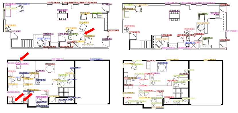
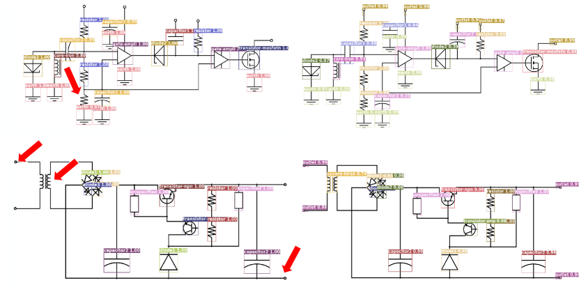
Figure 7: Qualitative comparison on floorplans and diagrams with YOLaT. The left column displays YOLaT’s results, while the right column showcases ours.

A.4 Additional Qualitative Evaluations

The results of additional cases are visually represented in this section, you can zoom in on each picture to capture more details, primitives belonging to different classes are represented in distinct colors. The color representations for each category can be referenced in Fig. 8. Some visualized results are shown in Fig. 9(a), Fig. 10(a) and Fig. 11(a) .

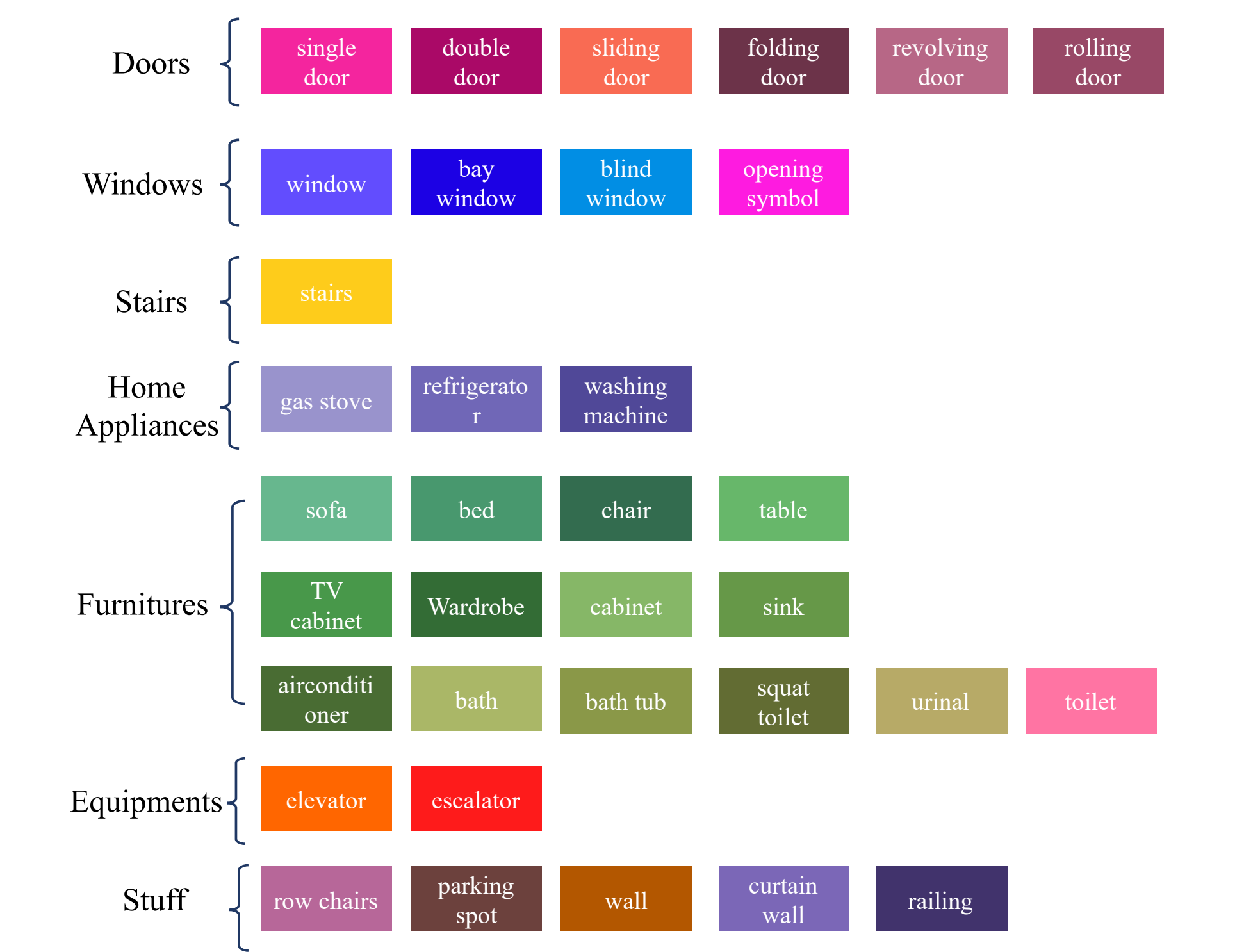
Figure 8: A visualized color map is provided for each class along with its corresponding super-class.

   

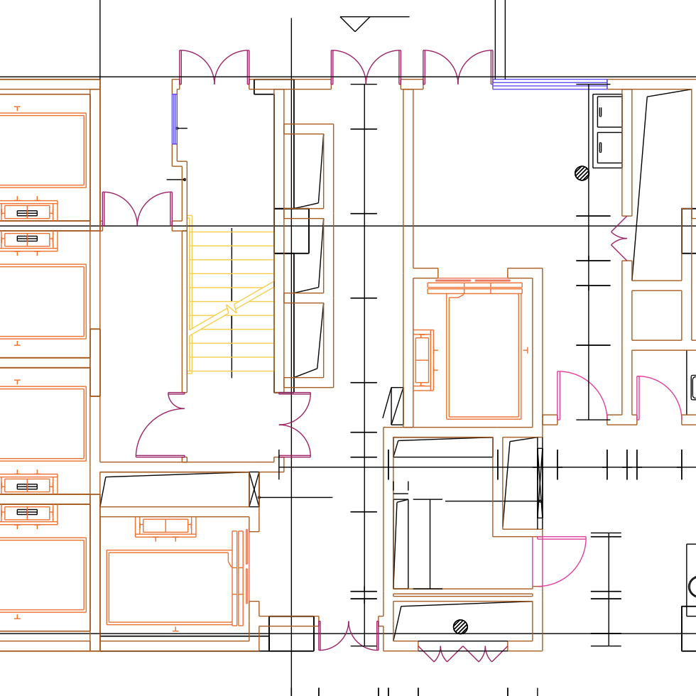
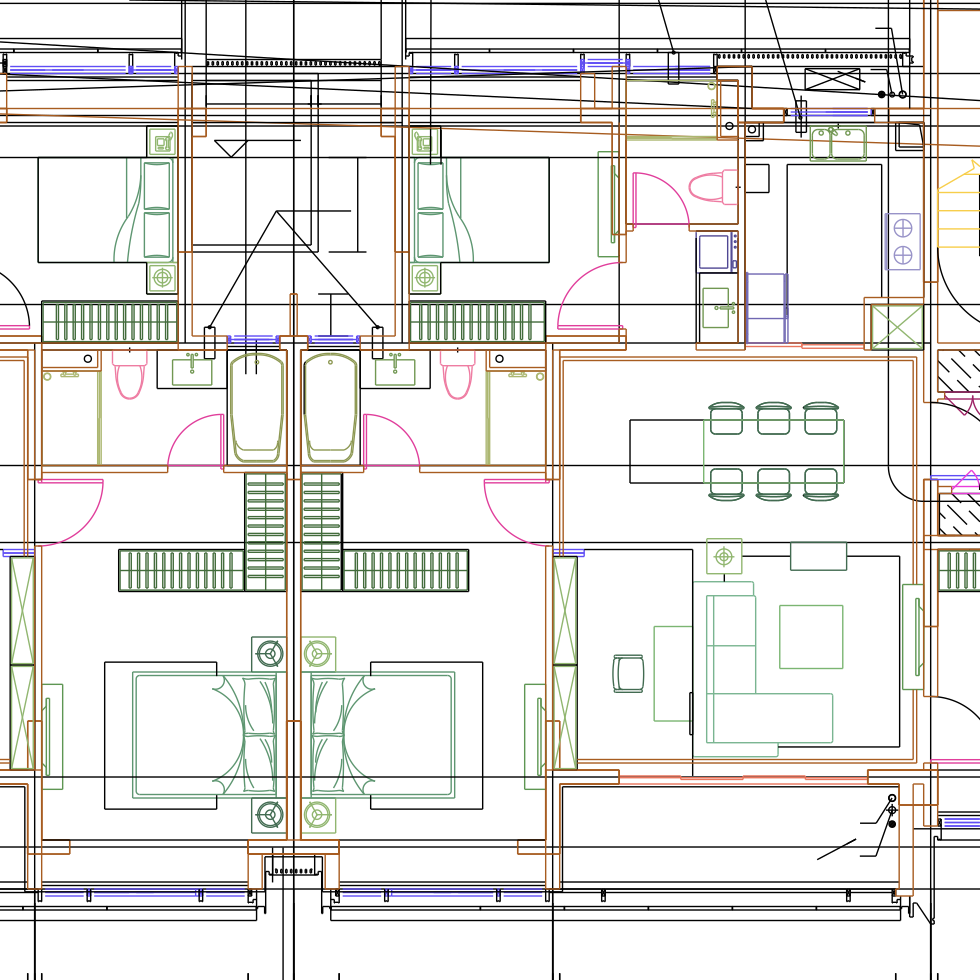
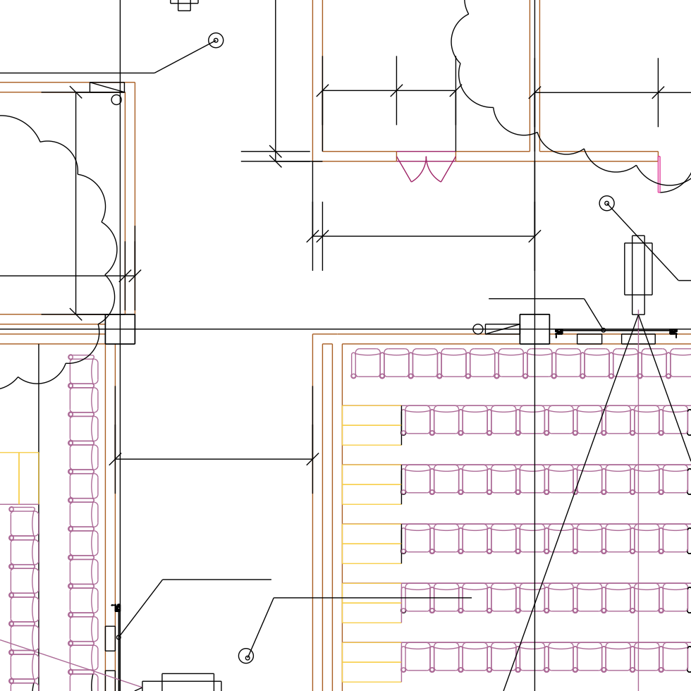
((a)) GT

   

((b)) SymPoint

Figure 9: Results of SymPoint on FloorPlanCAD.

 

   

((a)) GT

   

((b)) SymPoint

Figure 10: Results of SymPoint on FloorPlanCAD.

 

   

((a)) GT

   

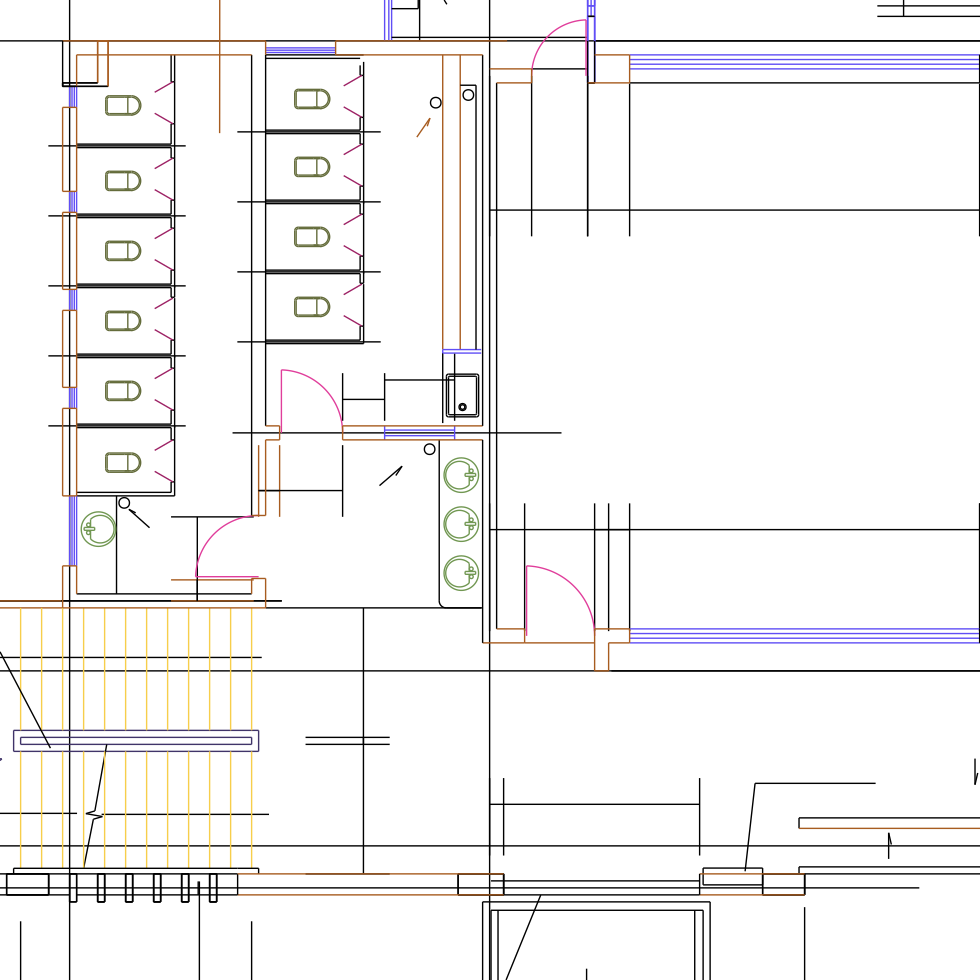
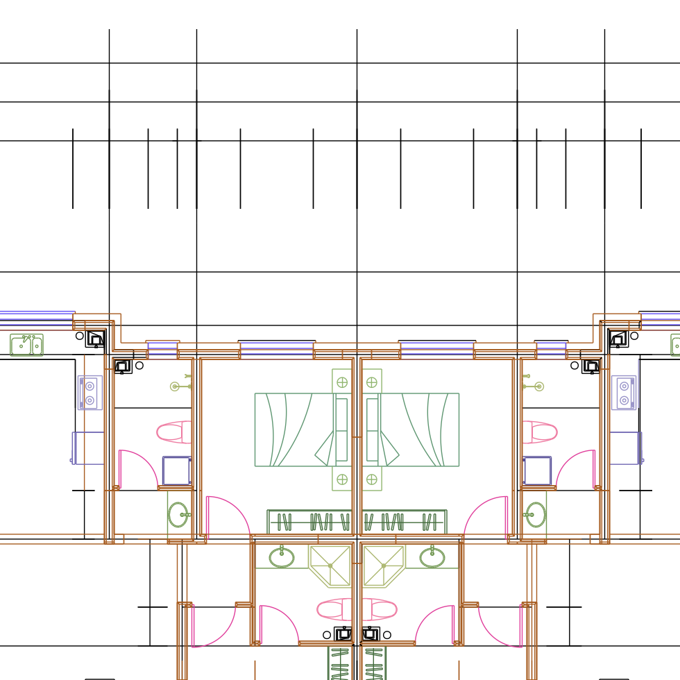
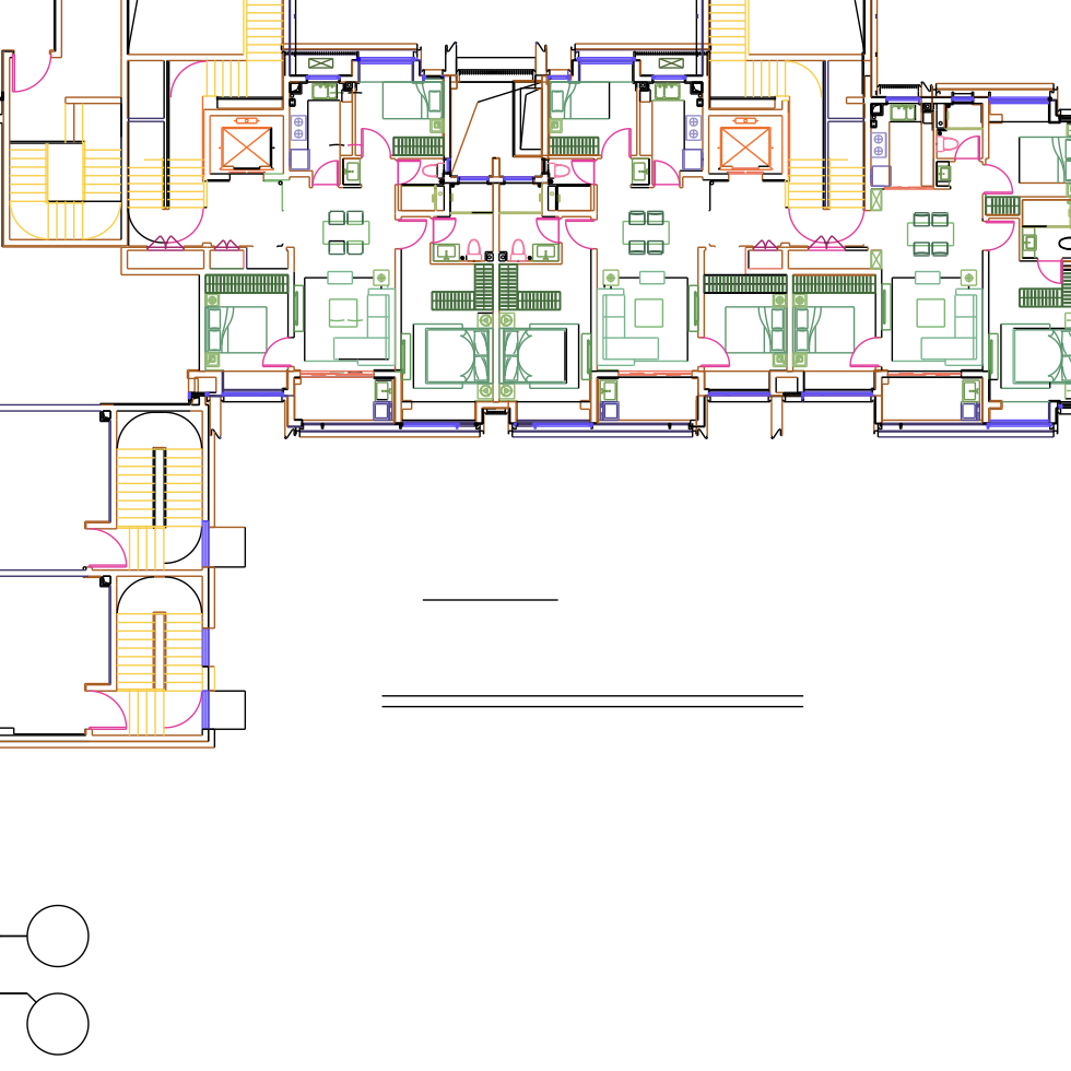
((b)) SymPoint

Figure 11: Results of SymPoint on FloorPlanCAD.

References

- Bochkovskiy et al. (2020) Alexey Bochkovskiy, Chien-Yao Wang, and Hong-Yuan Mark Liao. Yolov4: Optimal speed and accuracy of object detection. arXiv preprint arXiv:2004.10934, 2020.
- Carlier et al. (2020) Alexandre Carlier, Martin Danelljan, Alexandre Alahi, and Radu Timofte. Deepsvg: A hierarchical generative network for vector graphics animation. Advances in Neural Information Processing Systems, 33:16351–16361, 2020.
- Cheng et al. (2021) Bowen Cheng, Alex Schwing, and Alexander Kirillov. Per-pixel classification is not all you need for semantic segmentation. Advances in Neural Information Processing Systems, 34:17864–17875, 2021.
- Cheng et al. (2022) Bowen Cheng, Ishan Misra, Alexander G Schwing, Alexander Kirillov, and Rohit Girdhar. Masked-attention mask transformer for universal image segmentation. In Proceedings of the IEEE/CVF Conference on Computer Vision and Pattern Recognition, pp. 1290–1299, 2022.
- Cheng (1995) Yizong Cheng. Mean shift, mode seeking, and clustering. IEEE transactions on pattern analysis and machine intelligence, 17(8):790–799, 1995.
- Deng et al. (2018) Ruoxi Deng, Chunhua Shen, Shengjun Liu, Huibing Wang, and Xinru Liu. Learning to predict crisp boundaries. In Proceedings of the European conference on computer vision (ECCV), pp. 562–578, 2018.
- Fan et al. (2021) Zhiwen Fan, Lingjie Zhu, Honghua Li, Xiaohao Chen, Siyu Zhu, and Ping Tan. Floorplancad: A large-scale cad drawing dataset for panoptic symbol spotting. In Proceedings of the IEEE/CVF International Conference on Computer Vision, pp. 10128–10137, 2021.
- Fan et al. (2022) Zhiwen Fan, Tianlong Chen, Peihao Wang, and Zhangyang Wang. Cadtransformer: Panoptic symbol spotting transformer for cad drawings. In Proceedings of the IEEE/CVF Conference on Computer Vision and Pattern Recognition, pp. 10986–10996, 2022.
- Frosst et al. (2019) Nicholas Frosst, Nicolas Papernot, and Geoffrey Hinton. Analyzing and improving representations with the soft nearest neighbor loss. In International conference on machine learning, pp. 2012–2020. PMLR, 2019.
- Gutmann & Hyvärinen (2010) Michael Gutmann and Aapo Hyvärinen. Noise-contrastive estimation: A new estimation principle for unnormalized statistical models. In Proceedings of the thirteenth international conference on artificial intelligence and statistics, pp. 297–304. JMLR Workshop and Conference Proceedings, 2010.
- Hong et al. (2021) Fangzhou Hong, Hui Zhou, Xinge Zhu, Hongsheng Li, and Ziwei Liu. Lidar-based panoptic segmentation via dynamic shifting network. In Proceedings of the IEEE/CVF Conference on Computer Vision and Pattern Recognition, pp. 13090–13099, 2021.
- Jiang et al. (2021) Xinyang Jiang, Lu Liu, Caihua Shan, Yifei Shen, Xuanyi Dong, and Dongsheng Li. Recognizing vector graphics without rasterization. Advances in Neural Information Processing Systems, 34:24569–24580, 2021.
- Kirillov et al. (2019) Alexander Kirillov, Kaiming He, Ross Girshick, Carsten Rother, and Piotr Dollár. Panoptic segmentation. In Proceedings of the IEEE/CVF conference on computer vision and pattern recognition, pp. 9404–9413, 2019.
- Li et al. (2022) Jinke Li, Xiao He, Yang Wen, Yuan Gao, Xiaoqiang Cheng, and Dan Zhang. Panoptic-phnet: Towards real-time and high-precision lidar panoptic segmentation via clustering pseudo heatmap. In Proceedings of the IEEE/CVF Conference on Computer Vision and Pattern Recognition, pp. 11809–11818, 2022.
- Lin et al. (2017) Tsung-Yi Lin, Priya Goyal, Ross Girshick, Kaiming He, and Piotr Dollár. Focal loss for dense object detection. In Proceedings of the IEEE international conference on computer vision, pp. 2980–2988, 2017.
- Loshchilov & Hutter (2017) Ilya Loshchilov and Frank Hutter. Decoupled weight decay regularization. arXiv preprint arXiv:1711.05101, 2017.
- Ngo et al. (2023) Tuan Duc Ngo, Binh-Son Hua, and Khoi Nguyen. Isbnet: a 3d point cloud instance segmentation network with instance-aware sampling and box-aware dynamic convolution. In Proceedings of the IEEE/CVF Conference on Computer Vision and Pattern Recognition, pp. 13550–13559, 2023.
- Nguyen et al. (2009) Thi-Oanh Nguyen, Salvatore Tabbone, and Alain Boucher. A symbol spotting approach based on the vector model and a visual vocabulary. In 2009 10th International Conference on Document Analysis and Recognition, pp. 708–712. IEEE, 2009.
- Oord et al. (2018) Aaron van den Oord, Yazhe Li, and Oriol Vinyals. Representation learning with contrastive predictive coding. arXiv preprint arXiv:1807.03748, 2018.
- Qi et al. (2017a) Charles R Qi, Hao Su, Kaichun Mo, and Leonidas J Guibas. Pointnet: Deep learning on point sets for 3d classification and segmentation. In Proceedings of the IEEE conference on computer vision and pattern recognition, pp. 652–660, 2017a.
- Qi et al. (2017b) Charles Ruizhongtai Qi, Li Yi, Hao Su, and Leonidas J Guibas. Pointnet++: Deep hierarchical feature learning on point sets in a metric space. Advances in neural information processing systems, 30, 2017b.
- Reddy et al. (2021) Pradyumna Reddy, Michael Gharbi, Michal Lukac, and Niloy J Mitra. Im2vec: Synthesizing vector graphics without vector supervision. In Proceedings of the IEEE/CVF Conference on Computer Vision and Pattern Recognition, pp. 7342–7351, 2021.
- Redmon & Farhadi (2018) Joseph Redmon and Ali Farhadi. Yolov3: An incremental improvement. arXiv preprint arXiv:1804.02767, 2018.
- Ren et al. (2015) Shaoqing Ren, Kaiming He, Ross Girshick, and Jian Sun. Faster r-cnn: Towards real-time object detection with region proposal networks. Advances in neural information processing systems, 28, 2015.
- Rezvanifar et al. (2019) Alireza Rezvanifar, Melissa Cote, and Alexandra Branzan Albu. Symbol spotting for architectural drawings: state-of-the-art and new industry-driven developments. IPSJ Transactions on Computer Vision and Applications, 11:1–22, 2019.
- Rezvanifar et al. (2020) Alireza Rezvanifar, Melissa Cote, and Alexandra Branzan Albu. Symbol spotting on digital architectural floor plans using a deep learning-based framework. In Proceedings of the IEEE/CVF Conference on Computer Vision and Pattern Recognition Workshops, pp. 568–569, 2020.
- Schult et al. (2023) Jonas Schult, Francis Engelmann, Alexander Hermans, Or Litany, Siyu Tang, and Bastian Leibe. Mask3d: Mask transformer for 3d semantic instance segmentation. In 2023 IEEE International Conference on Robotics and Automation (ICRA), pp. 8216–8223. IEEE, 2023.
- Shi et al. (2022) Ruoxi Shi, Xinyang Jiang, Caihua Shan, Yansen Wang, and Dongsheng Li. Rendnet: Unified 2d/3d recognizer with latent space rendering. In Proceedings of the IEEE/CVF Conference on Computer Vision and Pattern Recognition, pp. 5408–5417, 2022.
- Sun et al. (2019) Ke Sun, Bin Xiao, Dong Liu, and Jingdong Wang. Deep high-resolution representation learning for human pose estimation. In Proceedings of the IEEE/CVF conference on computer vision and pattern recognition, pp. 5693–5703, 2019.
- Tian et al. (2019) Zhi Tian, Chunhua Shen, Hao Chen, and Tong He. Fcos: Fully convolutional one-stage object detection. In Proceedings of the IEEE/CVF international conference on computer vision, pp. 9627–9636, 2019.
- Xiao et al. (2023) Zeqi Xiao, Wenwei Zhang, Tai Wang, Chen Change Loy, Dahua Lin, and Jiangmiao Pang. Position-guided point cloud panoptic segmentation transformer. arXiv preprint arXiv:2303.13509, 2023.
- Yang et al. (2023) Bingchen Yang, Haiyong Jiang, Hao Pan, and Jun Xiao. Vectorfloorseg: Two-stream graph attention network for vectorized roughcast floorplan segmentation. In Proceedings of the IEEE/CVF Conference on Computer Vision and Pattern Recognition, pp. 1358–1367, 2023.
- Zhang et al. (2022) Hao Zhang, Feng Li, Shilong Liu, Lei Zhang, Hang Su, Jun Zhu, Lionel M Ni, and Heung-Yeung Shum. Dino: Detr with improved denoising anchor boxes for end-to-end object detection. arXiv preprint arXiv:2203.03605, 2022.
- Zhao et al. (2021) Hengshuang Zhao, Li Jiang, Jiaya Jia, Philip HS Torr, and Vladlen Koltun. Point transformer. In Proceedings of the IEEE/CVF international conference on computer vision, pp. 16259–16268, 2021.
- Zheng et al. (2022) Zhaohua Zheng, Jianfang Li, Lingjie Zhu, Honghua Li, Frank Petzold, and Ping Tan. Gat-cadnet: Graph attention network for panoptic symbol spotting in cad drawings. In Proceedings of the IEEE/CVF Conference on Computer Vision and Pattern Recognition, pp. 11747–11756, 2022.
- Zhou et al. (2021) Zixiang Zhou, Yang Zhang, and Hassan Foroosh. Panoptic-polarnet: Proposal-free lidar point cloud panoptic segmentation. In Proceedings of the IEEE/CVF Conference on Computer Vision and Pattern Recognition, pp. 13194–13203, 2021.