Computing Richelot isogeny graph of superspecial abelian threefolds

Abstract.

In algebraic geometry, superspecial curves are important research objects. While the number of superspecial genus-3 curves in characteristic $p$ is known, the number of hyperelliptic ones among them has not been determined even for small $p$. In this paper, in order to compute the latter number, we give an algorithm for computing the $(2,2,2)$-isogeny graph of superspecial abelian threefolds by using theta functions. This enables us to list up all superspecial genus-3 curves efficiently. Executing this algorithm on Magma, we succeeded in counting all superspecial hyperelliptic curves of genus $3$ when $11\leq p<100$, and in finding a single one when $7\leq p<10000$.

1. Introduction

Throughout this paper, by a curve we mean a non-singular projective variety of dimension one and isomorphisms between two curves are ones over an algebraically closed field. A curve $C$ over an algebraically closed field $k$ of characteristic $p>0$ is said to be superspecial if and only if the Jacobian of $C$ is isomorphic to the product of supersingular elliptic curves. Recently, superspecial curves are used for isogeny-based cryptography (e.g. [16], [5], [1] and so on), and then studies on such curves are becoming more important.

For given integers $g$ and $p$, it is known that the number of isomorphism classes of superspecial curves of genus $g$ in characteristic $p$ is finite, and determining that number is an important problem. This problem was already solved for genus $g\leq 3$; Deuring [11] found the number of all supersingular elliptic curves (i.e. $g=1$), and the number for $g=2$ is given by Ibukiyama, Katsura, and Oort [21]. For the case of $g=3$, Oort [34] and Ibukiyama [20] showed there exists a superspecial curve of genus $3$ in arbitrary characteristic $p\geq 3$, and the number of such curves was also computed by Brock [3]. However, the number of a superspecial hyperelliptic curve of genus 3 is not known, and in fact, even the existence of such a curve in arbitrary characteristic $p\geq 3$ has not been shown.

Our aim is to clarify the above problems for superspecial hyperelliptic curves of genus 3 in small characteristics $p$. For this, we use the connectivity of the Richelot isogeny graph of superspecial abelian varieties (see Section 2.4 for the definition), denoted by $\mathcal{G}_{g}(2,p)$. The computation of $\mathcal{G}_{2}(2,p)$ can be done using known formula (cf. [5, $\S 3$]), but there is no explicit formula in the case of $g\geq 3$. In this paper, we will describe an explicit algorithm for computing $\mathcal{G}_{3}(2,p)$ by using theta functions. Theta functions enable us to compute Richelot isogenies between abelian varieties as outlined in [9, Appendix F] and the case of $g=2$ was implemented by [10] indeed. However, since we want to obtain the graph $\mathcal{G}_{3}(2,p)$, our situation is a bit different from these cases. Therefore, we will prepare some formulae specific to our situation in Sections 2 and 3. One of our contributions is to write down how to identify the genus-3 curve from a theta null-point (see Sections 2.3 and 3.3 for details).

Consequently, we obtain the following main theorem:

Theorem 1.1.

Under some assumptions (see Remark 3.17 and Assumption 3.19), there is an algorithm (Algorithm 3.14) for computing the graph $\mathcal{G}_{3}(2,p)$ with $\widetilde{O}(p^{6})$ operations in the finite field $\hskip 0.85358pt\mathbb{F}_{p^{2}}$ for all chracteristics $p>7$.

Our algorithm allows us to restore the explicit defining equations of all superspecial curves of genus 3 efficiently, compared to the methods using the Gröbner basis (this complexity would be exponential with respect to $p$ in worst case).

Executing our algorithm, we succeeded in solving the existence of superspecial hyperelliptic curves of genus 3 in small $p$ as follows:

Theorem 1.2.

There exists a superspecial hyperelliptic curve of genus 3 in characteristic $p$ with $7\leq p<10000$. In addition, the numbers of isomorphism classes of such curves for $11\leq p<100$ are determined (as in Table 1 of Section 4.1).

We note that the upper bounds on $p$ in Theorem 1.2 can be increased easily. From our computational results, we obtain a conjecture that there exists a superspecial hyperelliptic curve of genus 3 in arbitrary characteristic $p\geq 7$.

The rest of this paper is organized as follows:  Section 2 is dedicated to reviewing some facts on analytic theta functions. In Section 2.4, we recall the definition and properties of superspecial Richelot isogeny graph $\mathcal{G}_{g}(2,p)$. We then explain how to compute the graph $\mathcal{G}_{3}(2,p)$ in Section 3, and finally Algorithm 3.14 gives its explicit construction. In Section 4, we state computational results about the existence and the number of superspecial hyperelliptic curves of genus 3 in small $p$, obtained by our implementation. At last, we give a concluding remark in Section 5.

Acknowledgements

This research was conducted under a contract of “Research and development on new generation cryptography for secure wireless communication services” among “Research and Development for Expansion of Radio Wave Resources (JPJ000254)”, which was supported by the Ministry of Internal Affairs and Communications, Japan. This work was supported by JSPS Grant-in-Aid for Young Scientists 20K14301 and 23K12949, and WISE program (MEXT) at Kyushu University.

2. Preliminaries

In this section, we summarize background knowledge required in later sections. Abelian varieties and isogenies between them until Section 2.3 are defined over $\mathbb{C}$, but in Section 2.4 we consider those over a field of odd characteristic.

2.1. Abelian varieties and their isogenies

In this subsection, we review about complex abelian varieties and isogenies. A complex abelian variety  of dimension $g$ is isomorphic to $\mathbb{C}^{g}/(\mathbb{Z}^{g}+\varOmega\mathbb{Z}^{g})$ where $\varOmega$ is an element of the Siegel upper half-space

$$\mathcal{H}_{g}\coloneqq\{\varOmega\in{\rm Mat}_{g}(\mathbb{C})\,\mid\,^{t}\varOmega=\varOmega,\,{\rm Im}\,\varOmega>0\}.\vspace{0.5mm}$$

Then, we call $\varOmega\in\mathcal{H}_{g}$ a period matrix of the abelian variety. First of all, we recall a characterization of isomorphisms between abelian varieties:

Definition 2.1.

For a commutative ring $R$ and an integer $g\geq 1$, we define a group

$${\rm Sp}_{2g}(R)\coloneqq\{M\in{\rm GL}_{2g}(R)\,\mid\,ME\hskip 0.85358pt^{t}M=E\},\quad E\coloneqq\begin{pmatrix}0&{\mathbf{1}}_{g}\\ -{\mathbf{1}}_{g}&0\end{pmatrix}.$$

We say that a matrix $M\in{\rm GL}_{2g}(R)$ is symplectic over $R\hskip 0.56905pt$ if $M\in{\rm Sp}_{2g}(R)$.

The following lemma helps determine whether $M$ is a symplectic matrix or not:

Lemma 2.2 ([28, Lemma 8.2.1]).

For any $(2g\times 2g)$-matrix $M=\begin{pmatrix}\alpha&\beta\\[-0.85358pt] \gamma&\delta\end{pmatrix}\in{\rm GL}_{2g}(R)$ with $\alpha,\beta,\gamma,\delta\in{\rm Mat}_{g}(R)$, the following three statements are equivalent:

1. The matrix $M$ is symplectic over $R$.

2. Two matrices $\alpha\hskip 0.56905pt^{t}\beta,\,\gamma\hskip 0.85358pt^{t}\delta$ are both symmetric and $\alpha\hskip 0.85358pt^{t}\delta-\beta\hskip 1.42262pt^{t}\gamma={\mathbf{1}}_{g}$.

3. Two matrices ${}^{t}\alpha\hskip 0.85358pt\gamma,\hskip 1.42262pt^{t}\beta\hskip 1.42262pt\delta$ are both symmetric and ${}^{t}\alpha\hskip 0.85358pt\delta-\hskip 1.42262pt^{t}\beta\hskip 1.42262pt\gamma={\mathbf{1}}_{g}$.

For a matrix $M=\begin{pmatrix}\alpha&\beta\\[-0.85358pt] \gamma&\delta\end{pmatrix}\in{\rm Sp}_{2g}(\mathbb{Z})$, the action on the Siegel upper half-space

$$\begin{split}{\rm Sp}_{2g}(\mathbb{Z})\times\mathcal{H}_{g}&\longrightarrow\mathcal{H}_{g}\\[-1.42262pt] (M,\varOmega)&\longmapsto(\alpha\varOmega+\beta)(\gamma\varOmega+\delta)^{-1}\eqqcolon M.\varOmega\end{split}$$

is well-defined. Moreover, the map

$$\mathbb{C}^{g}\longrightarrow\mathbb{C}^{g}\,;\,z\longmapsto^{t}(\gamma\varOmega+\delta)^{-1}z\eqqcolon M.z\vspace{0.5mm}$$

induces an isomorphism $\mathbb{C}^{g}/(\mathbb{Z}^{g}+\varOmega\mathbb{Z}^{g})\rightarrow\mathbb{C}^{g}/(\mathbb{Z}^{g}+M.\varOmega\mathbb{Z}^{g})$.

Theorem 2.3 ([28, Theorem 8.3.1]).

Two matrices $\varOmega,\varOmega^{\prime}\in\mathcal{H}_{g}$ determine isomorphic abelian varieties if and only if there exists $M\in{\rm Sp}_{2g}(\mathbb{Z})$ such that $\varOmega^{\prime}=M.\varOmega$.

An isogeny is a surjective homomorphism between two abelian varieties. If there exists an isogeny $A\rightarrow B$, then the dimensions of $A$ and $B$ are equal to each other, and we say that $A$ and $B$ are isogenous. Two isogenies $A\rightarrow B$ with the same kernel are equivalent up to an automorphism of $B$, and thus we identify them.

Proposition 2.4.

For an abelian variety $A$ of dimension $g$ and a prime integer $\ell$, the number of maximal isotropic subgroups $G$ of $A[\ell]$ is equal to

$$N_{g}(\ell)\coloneqq\prod_{k=1}^{g}(\ell^{k}+1).$$

Proof.

See [8, Lemma 2] or [4, Lemma 2]. ∎

An isogeny whose kernel is such a group $G$ the above is called an $(\overbrace{\ell,\dots,\ell}^{g})$-isogeny. In particular, one can see that the $(\ell,\ldots,\ell)$-isogeny

$$\begin{split}\mathbb{C}^{g}/(\mathbb{Z}^{g}+\varOmega\mathbb{Z}^{g})&\longrightarrow\mathbb{C}^{g}/(\mathbb{Z}^{g}+\ell\varOmega\mathbb{Z}^{g})\\[-1.42262pt] z&\longmapsto\ell z\end{split}$$

has the kernel $\frac{1}{\ell}\mathbb{Z}^{g}/\mathbb{Z}^{g}$.

2.2. Theta functions

The theta function of characteristics $a,b\in\mathbb{Q}^{g}$ is given as

$$\theta\bigl{[}\begin{smallmatrix}a\\ b\end{smallmatrix}\bigr{]}(z,\varOmega)\coloneqq\sum_{n\in\mathbb{Z}^{g}}\exp\bigl{(}\pi i\hskip 1.42262pt^{t}(n+a)\hskip 0.56905pt\varOmega\hskip 0.56905pt(n+a)+2\pi i\hskip 1.42262pt^{t}(n+a)(z+b)\bigr{)}\vspace{0.5mm}$$

for $z\in\mathbb{C}^{g}$ and $\varOmega\in\mathcal{H}_{g}$. All the characteristics can be considered modulo $\mathbb{Z}^{g}$ since one can check that

$$\theta\bigl{[}\begin{smallmatrix}a+\alpha\\ b+\beta\end{smallmatrix}\bigr{]}(z,\varOmega)=\theta\bigl{[}\begin{smallmatrix}a\\ b\end{smallmatrix}\bigr{]}(z,\varOmega)\exp(2\pi i\hskip 1.42262pt^{t}a\beta)$$

for all $\alpha,\beta\in\mathbb{Z}^{g}$. Then, in the paper, we consider only theta functions $\theta\bigl{[}\begin{smallmatrix}a\\ b\end{smallmatrix}\bigr{]}(z,\varOmega)$ for characteristics $a,b\in\frac{1}{2}\mathbb{Z}^{g}/\mathbb{Z}^{g}$.

Lemma 2.5.

For all characteristics $a,b\in\frac{1}{2}\mathbb{Z}^{g}/\mathbb{Z}^{g}$, the function $\theta\bigl{[}\begin{smallmatrix}a\\ b\end{smallmatrix}\bigr{]}(z,\varOmega)$ is even with respect to $z$ if and only if $4\hskip 0.56905pt^{t}ab$ is an even integer;  otherwise $\theta\bigl{[}\begin{smallmatrix}a\\ b\end{smallmatrix}\bigr{]}(z,\varOmega)$ is odd.

Proof.

The first assertion follows from that

$$\theta\bigl{[}\begin{smallmatrix}a\\ b\end{smallmatrix}\bigr{]}(-z,\varOmega)=(-1)^{4\hskip 0.56905pt^{t}ab}\theta\bigl{[}\begin{smallmatrix}a\\ b\end{smallmatrix}\bigr{]}(z,\varOmega).$$

The second assertion follows from that $4\hskip 0.56905pt^{t}ab$ is an integer for all $a,b\in\frac{1}{2}\mathbb{Z}^{g}/\mathbb{Z}^{g}$. ∎

The following two formulas are very fundamental and generate many relations:

Theorem 2.6 (Riemann’s theta formula).

Let $m_{k}:=\begin{pmatrix}a_{k}\\ b_{k}\end{pmatrix}$ with $a_{k},b_{k}\in\frac{1}{2}\mathbb{Z}^{g}/\mathbb{Z}^{g}$, and we define

$$\begin{pmatrix}n_{1}\\ n_{2}\\ n_{3}\\ n_{4}\end{pmatrix}\coloneqq\hskip 0.85358pt\frac{1}{2}\begin{pmatrix}{\mathbf{1}}_{2g}&\hskip 7.68222pt{\mathbf{1}}_{2g}&\hskip 7.68222pt{\mathbf{1}}_{2g}&\hskip 7.68222pt{\mathbf{1}}_{2g}\\ {\mathbf{1}}_{2g}&\hskip 7.68222pt{\mathbf{1}}_{2g}&-{\mathbf{1}}_{2g}&-{\mathbf{1}}_{2g}\\ {\mathbf{1}}_{2g}&-{\mathbf{1}}_{2g}&\hskip 7.68222pt{\mathbf{1}}_{2g}&-{\mathbf{1}}_{2g}\\ {\mathbf{1}}_{2g}&-{\mathbf{1}}_{2g}&-{\mathbf{1}}_{2g}&\hskip 7.68222pt{\mathbf{1}}_{2g}\end{pmatrix}\begin{pmatrix}m_{1}\\ m_{2}\\ m_{3}\\ m_{4}\end{pmatrix}.$$

Then, we have the equation

$$\prod_{k=1}^{4}\theta[m_{k}](0,\varOmega)=\frac{1}{2^{g}}\sum_{\alpha,\beta\in\frac{1}{2}\mathbb{Z}^{g}/\mathbb{Z}^{g}}(-1)^{4\hskip 0.56905pt^{t}a\beta}\prod_{k=1}^{4}\theta[n_{k}+\gamma_{\alpha,\beta}](0,\varOmega)\vspace{0.5mm}$$

where $\gamma_{\alpha,\beta}$ denotes $\begin{pmatrix}\alpha\\ \beta\end{pmatrix}$ with $\alpha,\beta\in\frac{1}{2}\mathbb{Z}^{g}/\mathbb{Z}^{g}$.

Proof.

Apply [23, Chapter IV, Theorem 1] for $z_{1}=z_{2}=z_{3}=z_{4}=0$. ∎

Theorem 2.7 (Duplication formula).

For all $a,b\in\frac{1}{2}\mathbb{Z}^{g}/\mathbb{Z}^{g}$, we have

$$\theta\bigl{[}\begin{smallmatrix}a\\ b\end{smallmatrix}\bigr{]}(z,\varOmega)^{2}=\frac{1}{2^{g}}\hskip 0.56905pt\sum_{\beta\in\frac{1}{2}\mathbb{Z}^{g}/\mathbb{Z}^{g}}(-1)^{4\hskip 0.56905pt^{t}a\beta}\hskip 0.85358pt\theta\bigl{[}\begin{smallmatrix}0\\ b\end{smallmatrix}\bigr{]}(z,\varOmega/2)\theta\bigl{[}\begin{smallmatrix}0\\ b+\beta\end{smallmatrix}\bigr{]}(z,\varOmega/2).$$

Proof.

Apply [23, Chapter IV, Theorem 2] for $m_{1}=m_{2}$ and $z_{1}=z_{2}=z$. ∎

Especially if a matrix $\varOmega\in\mathcal{H}_{g}$ is written as

$$\varOmega=\begin{pmatrix}\varOmega_{1}&0\\ 0&\varOmega_{2}\end{pmatrix}\ \,{\rm where}\ \,\varOmega_{1}\in\mathcal{H}_{g_{1}},\ \varOmega_{2}\in\mathcal{H}_{g_{2}}$$

with $g_{1}+g_{2}=g$, then we have the following lemma:

Lemma 2.8 ([9, Lemma F.3.1]).

With notations the above, we write $z=(z_{1},z_{2})$ where $z_{1}\in\mathbb{C}^{g_{1}},\,z_{2}\in\mathbb{C}^{g_{2}}$. Then, we have the equation

$$\theta\bigl{[}\begin{smallmatrix}a_{1}&a_{2}\\ b_{1}&b_{2}\end{smallmatrix}\bigr{]}(z,\varOmega)=\theta\bigl{[}\begin{smallmatrix}a_{1}\\ b_{1}\end{smallmatrix}\bigr{]}(z_{1},\varOmega_{1})\hskip 0.85358pt\theta\bigl{[}\begin{smallmatrix}a_{2}\\ b_{2}\end{smallmatrix}\bigr{]}(z_{2},\varOmega_{2})\vspace{0.5mm}$$

for all characteristics $a_{1},b_{1}\in\frac{1}{2}\mathbb{Z}^{g_{1}}/\mathbb{Z}^{g_{1}}$ and $a_{2},b_{2}\in\frac{1}{2}\mathbb{Z}^{g_{2}}/\mathbb{Z}^{g_{2}}$.

Let us return to cases with a general (not necessarily diagonal) matrix $\varOmega\in\mathcal{H}_{g}$. For any symplectic matrix $M=\begin{pmatrix}\alpha&\beta\\[-0.85358pt] \gamma&\delta\end{pmatrix}\in{\rm Sp}_{2g}(\mathbb{Z})$ and characteristics $a,b\in\frac{1}{2}\mathbb{Z}^{g}/\mathbb{Z}^{g}$, we define a scalar

$$k(M,a,b):=(a\hskip 0.85358pt^{t}\delta-b\hskip 1.13809pt^{t}\gamma)\hskip 1.42262pt\cdot\hskip 0.85358pt^{t}(b\hskip 1.42262pt^{t}\alpha-a\hskip 0.85358pt^{t}\beta+(\alpha\hskip 0.85358pt^{t}\beta)_{0})-a\hskip 0.85358pt^{t}b\vspace{0.5mm}$$

and two vectors

(2.1) $$M.a:=a\hskip 0.85358pt^{t}\delta-b\hskip 1.13809pt^{t}\gamma+\frac{1}{2}(\gamma\hskip 1.42262pt^{t}\delta)_{0},\quad M.b:=b\hskip 1.42262pt^{t}\alpha-a\hskip 0.85358pt^{t}\beta+\frac{1}{2}(\alpha\hskip 0.85358pt^{t}\beta)_{0},\vspace{0.5mm}$$

where $(\alpha\hskip 0.85358pt^{t}\beta)_{0},(\gamma\hskip 1.42262pt^{t}\delta)_{0}$ denote the row vector of the diagonal elements of $(\alpha\hskip 0.85358pt^{t}\beta),(\gamma\hskip 1.42262pt^{t}\delta)$. Then, the matrix $M$ acts on the theta function in the following way:

Theorem 2.9 (Theta transformation formula).

For all $a,b\in\frac{1}{2}\mathbb{Z}^{g}/\mathbb{Z}^{g}$, we have

$$\theta\bigl{[}\begin{smallmatrix}M.a\\ M.b\end{smallmatrix}\bigr{]}(M.z,M.\varOmega)=c\cdot e^{\pi ik(M,a,b)}\theta\bigl{[}\begin{smallmatrix}a\\ b\end{smallmatrix}\bigr{]}(z,\varOmega),\vspace{1mm}$$

where $c\in\mathbb{C}^{\times}$ is a constant which does not depend $a$ or $b$.

Proof.

This follows from [28, Theorem 8.6.1]. ∎

Let $n\geq 1$ be an integer and we define

$$\varGamma_{n} :=\bigl{\{}M=\begin{pmatrix}\alpha&\beta\\[-0.85358pt] \gamma&\delta\end{pmatrix}\in{\rm Sp}_{2g}(\mathbb{Z})\,\mid\,\alpha\equiv\delta\equiv{\mathbf{1}}_{g},\ \beta\equiv\gamma\equiv{\mathbf{0}}_{g}\pmod{n}\bigr{\}},$$

$$\varGamma_{n,2n} :=\bigl{\{}M=\begin{pmatrix}\alpha&\beta\\[-0.85358pt] \gamma&\delta\end{pmatrix}\in\varGamma_{n}\,\mid\,{\rm diag}(\hskip 0.85358pt^{t}\alpha\gamma)\equiv{\rm diag}(\hskip 0.85358pt^{t}\beta\hskip 0.85358pt\delta)\equiv 0\pmod{2n}\},$$

which are both subgroups of ${\rm Sp}_{2g}(\mathbb{Z})$.

Corollary 2.10.

For all characteristics $a,b\in\frac{1}{2}\mathbb{Z}^{g}/\mathbb{Z}^{g}$, we have

$$\frac{\theta\bigl{[}\begin{smallmatrix}a\\ b\end{smallmatrix}\bigr{]}(0,M.\varOmega)^{4}}{\theta\bigl{[}\begin{smallmatrix}0\\ 0\end{smallmatrix}\bigr{]}(0,M.\varOmega)^{4}} =\frac{\theta\bigl{[}\begin{smallmatrix}a\\ b\end{smallmatrix}\bigr{]}(0,\varOmega)^{4}}{\theta\bigl{[}\begin{smallmatrix}0\\ 0\end{smallmatrix}\bigr{]}(0,\varOmega)^{4}}\quad{\rm if}\ M\in\varGamma_{2},$$

$$\frac{\theta\bigl{[}\begin{smallmatrix}a\\ b\end{smallmatrix}\bigr{]}(0,M.\varOmega)^{2}}{\theta\bigl{[}\begin{smallmatrix}0\\ 0\end{smallmatrix}\bigr{]}(0,M.\varOmega)^{2}} =\frac{\theta\bigl{[}\begin{smallmatrix}a\\ b\end{smallmatrix}\bigr{]}(0,\varOmega)^{2}}{\theta\bigl{[}\begin{smallmatrix}0\\ 0\end{smallmatrix}\bigr{]}(0,\varOmega)^{2}}\quad{\rm if}\ M\in\varGamma_{2,4},$$

$$\frac{\theta\bigl{[}\begin{smallmatrix}a\\ b\end{smallmatrix}\bigr{]}(0,M.\varOmega)}{\theta\bigl{[}\begin{smallmatrix}0\\ 0\end{smallmatrix}\bigr{]}(0,M.\varOmega)} =\frac{\theta\bigl{[}\begin{smallmatrix}a\\ b\end{smallmatrix}\bigr{]}(0,\varOmega)}{\theta\bigl{[}\begin{smallmatrix}0\\ 0\end{smallmatrix}\bigr{]}(0,\varOmega)}\quad\ \,{\rm if}\ M\in\varGamma_{4,8}.$$

Proof.

It follows from Theorem 2.9 that

$$\frac{\theta\bigl{[}\begin{smallmatrix}a\\ b\end{smallmatrix}\bigr{]}(0,M.\varOmega)}{\theta\bigl{[}\begin{smallmatrix}0\\ 0\end{smallmatrix}\bigr{]}(0,M.\varOmega)}=\frac{\theta\bigl{[}\begin{smallmatrix}a\\ b\end{smallmatrix}\bigr{]}(0,\varOmega)}{\theta\bigl{[}\begin{smallmatrix}0\\ 0\end{smallmatrix}\bigr{]}(0,\varOmega)}\exp\bigl{(}\pi ia\hskip 0.85358pt^{t}\beta\hskip 0.85358pt\delta\hskip 1.42262pt^{t}a-\pi ib\hskip 0.85358pt^{t}\gamma\hskip 0.85358pt\alpha\hskip 1.42262pt^{t}b-2\pi ia(\hskip 0.56905pt^{t}\alpha-\mathbf{1}_{g})\hskip 0.56905pt^{t}b\bigr{)}.$$

Hence, we obtain this assertion by simple computations. ∎

2.3. Theta functions for abelian threefolds

In this subsection, we focus only on the case that $A$ is an abelian threefold (i.e.  abelian variety of dimension $g=3$), and we discuss theta functions associated to $A$. According to [28, Corollary 11.8.2], such $A$ is either of the following 4 types.

$$\begin{split}\left\{\begin{array}[]{l}{\rm Type\ 1\!:\ }\,A\cong{\rm Jac}(C)\ \text{where}\ C\ \text{is\ a\ smooth\ plane\ quartic},\\[1.42262pt] {\rm Type\ 2\!:\ }\,A\cong{\rm Jac}(C)\ \text{where}\ C\ \text{is\ a\ hyperelliptic\ curve\ of\ genus\ }3,\\[1.42262pt] {\rm Type\ 3\!:\ }\,A\cong E\times{\rm Jac}(C)\ \text{where}\ E\ \text{and}\ C\text{\ is\ a genus-1 and genus-2 curve},\\[1.42262pt] {\rm Type\ 4\!:\ }\,A\cong E_{1}\times E_{2}\times E_{3}\ \text{where}\ E_{1},E_{2}\text{\ and\ }E_{3}\text{\ are\ elliptic\ curves}.\end{array}\right.\vspace{0.5mm}\end{split}$$

First of all, we introduce the following notations for the sake of simplicity.

Definition 2.11.

For a period matrix $\varOmega\in\mathcal{H}_{3}$ of $A$, we write

$$\vartheta_{i}(z,\varOmega):=\theta\bigl{[}\begin{smallmatrix}a_{1}&a_{2}&a_{3}\\ b_{1}&b_{2}&b_{3}\end{smallmatrix}\bigr{]}(z,\varOmega),\quad i:=2b_{1}+4b_{2}+8b_{3}+16a_{1}+32a_{2}+64a_{3},\vspace{0.5mm}$$

where $a_{1},a_{2},a_{3},b_{1},b_{2}$, and $b_{3}$ belong to $\{0,1/2\}$. Note that $i$ runs over $\{0,\ldots,63\}$. Moreover, the value $\vartheta_{i}(0,\varOmega)$ is simply be denoted as $\vartheta_{i}$.

We consider an abelian threefold $A\cong\mathbb{C}^{3}/(\mathbb{Z}^{3}+\varOmega\mathbb{Z}^{3})$, then the projective value

$$[\vartheta_{0}^{2}:\vartheta_{1}^{2}:\cdots:\vartheta_{63}^{2}]\in\mathbb{P}^{63}(\mathbb{C})\vspace{0.5mm}$$

is called a theta null-point of $A$. Remark that there are different theta null-points for isomorphic abelian threefolds.

Definition 2.12.

We define the sets

$$I_{\rm even}\coloneqq\left\{\begin{array}[]{l}0,\,1,\,2,\,3,\,4,\,5,\,6,\,7,\,8,\,10,\,12,\,14,\,16,\,17,\,20,\,21,\,24,\,27,\,28,\\ 31,\,32,\,33,\,34,\,35,\,40,\,42,\,45,\,47,\,48,\,49,\,54,\,55,\,56,\,59,\,61,\,62\end{array}\right\}$$

and $I_{\rm odd}\coloneqq\{0,\ldots,63\}\smallsetminus I_{\rm even}$. Here, we remark that $\#I_{\rm even}=36$ and $\#I_{\rm odd}=28$.

It follows from Lemma 2.5 that $\vartheta_{i}(z)$ is even (resp. odd) if and only if $i\in I_{\rm even}$ (resp. $i\in I_{\rm odd}$). Therefore, we have that $\vartheta_{i}=0$ for all $i\in I_{\rm odd}$.

Definition 2.13.

Let $S_{\rm van}$ be the set of vanishing indices $i\in I_{\rm even}$, that is,

$$S_{\rm van}\coloneqq\{\hskip 0.56905pti\in I_{\rm even}\mid\vartheta_{i}=0\}.$$

In addition, we denote by $N_{\rm van}$ the cardinality of the set $S_{\rm van}$.

Lemma 2.14.

The value $N_{\rm van}$ is invariant for isomorphic abelian threefolds.

Proof.

This follows from the theta transformation formula (Theorem 2.9). ∎

Then, we can identify by $N_{\rm van}$ which of the above 4 types $A$ corresponds (remark that this does not depend on a period matrix $\varOmega$ of $A$ by the above lemma).

Proposition 2.15.

The possible values of $N_{\rm van}$ are $0,1,6,9$ and moreover

$$\left\{\begin{array}[]{l}N_{\rm van}=0\ \Leftrightarrow\,A\cong{\rm Jac}(C)\ \text{where}\ C\ \text{is\ a\ smooth\ plane\ quartic},\\[1.42262pt] N_{\rm van}=1\ \Leftrightarrow\,A\cong{\rm Jac}(C)\ \text{where}\ C\ \text{is\ a\ hyperelliptic\ curve\ of\ genus\ }3,\\[1.42262pt] N_{\rm van}=6\ \Leftrightarrow\,A\cong E\times{\rm Jac}(C)\ \text{where}\ E\ \text{and}\ C\text{\ is\ a genus-1 and genus-2 curve},\\[1.42262pt] N_{\rm van}=9\ \Leftrightarrow\,A\cong E_{1}\times E_{2}\times E_{3}\ \text{where}\ E_{1},E_{2}\text{\ and\ }E_{3}\text{\ are\ elliptic\ curves}.\end{array}\right.$$

Proof.

The first assertion follows from [18, Theorem 3.1] (the cases where $N_{\rm van}>9$ correspond to singular abelian threefolds). The second assertion for $N_{\rm van}=0,1$ are shown by [35, Theorem 2], and hence we show the remaining cases.

Let $A$ be an abelian threefold such that $A$ is isomorphic to the product $A_{1}\times A_{2}$ of an elliptic curve $A_{1}$ and an abelian surface $A_{2}$. Denote $\varOmega_{1},\varOmega_{2}$ and $\varOmega$ be one of period matrices of $A_{1},A_{2}$ and $A$, respectively. Then, there exists $M\in{\rm Sp}_{6}(\mathbb{Z})$ such that $M.\varOmega={\rm diag}(\varOmega_{1},\varOmega_{2})$ from Theorem 2.3, but we may assume $\varOmega={\rm diag}(\varOmega_{1},\varOmega_{2})$ by using Lemma 2.14. It follows from Lemma 2.8 that

$$\theta\bigl{[}\begin{smallmatrix}a_{1}&a_{2}&a_{3}\\ b_{1}&b_{2}&b_{3}\end{smallmatrix}\bigr{]}(z,\varOmega)=\theta\bigl{[}\begin{smallmatrix}a_{1}\\ b_{1}\end{smallmatrix}\bigr{]}(z_{1},\varOmega_{1})\hskip 0.85358pt\theta\bigl{[}\begin{smallmatrix}a_{2}&a_{3}\\ b_{2}&b_{3}\end{smallmatrix}\bigr{]}(z_{2},\varOmega_{2}),\quad z\coloneqq(z_{1},z_{2}),\vspace{0.5mm}$$

and hence we see that $N_{\rm van}=6$ (resp.  $9$) if $A_{2}$ is simple (resp. not simple). ∎

At the rest of this subsection, we assume that an abelian threefold $A$ corresponds to a genus-3 curve $C$. Let us review how to restore a defining equation of $C$ in the case that $C$ is hyperelliptic.

Proposition 2.16.

We assume that $S_{\rm van}=\{61\}$ for a period matrix $\varOmega\in\mathcal{H}_{3}$ of $A$. Then $A$ is isomorphic to the Jacobian of a genus-3 hyperelliptic curve

$$C:y^{2}=x(x-1)(x-\lambda_{1})(x-\lambda_{2})(x-\lambda_{3})(x-\lambda_{4})(x-\lambda_{5}),$$

where

(2.2) $$\lambda_{1}\coloneqq\frac{\vartheta_{42}^{2}\vartheta_{2}^{2}}{\vartheta_{5}^{2}\vartheta_{45}^{2}},\ \,\lambda_{2}\coloneqq\frac{\vartheta_{42}^{2}\vartheta_{3}^{2}}{\vartheta_{4}^{2}\vartheta_{45}^{2}},\ \,\lambda_{3}\coloneqq\frac{\vartheta_{27}^{2}\vartheta_{42}^{2}}{\vartheta_{45}^{2}\vartheta_{28}^{2}},\ \,\lambda_{4}\coloneqq\frac{\vartheta_{2}^{2}\vartheta_{49}^{2}}{\vartheta_{54}^{2}\vartheta_{5}^{2}},\ \,\lambda_{5}\coloneqq\frac{\vartheta_{3}^{2}\vartheta_{0}^{2}}{\vartheta_{7}^{2}\vartheta_{4}^{2}}.$$

Proof.

Apply Thomae’s formula (cf. [39]) for $g=3$ or see [36, Theorem 4]. ∎

On the other hand, even in the case that $C$ is a plane quartic, we can also restore an explicit equation of $C$. Taking a period matrix $\varOmega\in\mathcal{H}_{3}$ of $A={\rm Jac}(C)$, then it follows from Proposition 2.15 that $\vartheta_{i}\neq 0$ for all $i\in I_{\rm even}$. We define the following non-zero values

$$a_{11} \coloneqq\frac{\vartheta_{12}\vartheta_{5}}{\vartheta_{40}\vartheta_{33}}, \quad a_{21} \coloneqq\frac{\vartheta_{27}\vartheta_{5}}{\vartheta_{40}\vartheta_{54}}, \quad a_{31} \coloneqq-\frac{\vartheta_{27}\vartheta_{12}}{\vartheta_{33}\vartheta_{54}},$$

(2.3) $$a_{12} \coloneqq\frac{\vartheta_{21}\vartheta_{28}}{\vartheta_{49}\vartheta_{56}}, \quad a_{22} \coloneqq\frac{\vartheta_{2}\vartheta_{28}}{\vartheta_{49}\vartheta_{47}}, \quad a_{32} \coloneqq\frac{\vartheta_{2}\vartheta_{21}}{\vartheta_{56}\vartheta_{47}},$$

$$a_{13} \coloneqq\frac{\vartheta_{7}\vartheta_{14}}{\vartheta_{35}\vartheta_{42}}, \quad a_{23} \coloneqq\frac{\vartheta_{16}\vartheta_{14}}{\vartheta_{35}\vartheta_{61}}, \quad a_{33} \coloneqq\frac{\vartheta_{16}\vartheta_{7}}{\vartheta_{42}\vartheta_{61}}$$

computed as in [13, p. 15]. Then, there exist $k_{1},k_{2},k_{3},\lambda_{1},\lambda_{2},\lambda_{3}\in\mathbb{C}^{\times}$ such that

(2.4) $$\begin{pmatrix}\lambda_{1}a_{11}&\lambda_{2}a_{21}&\lambda_{3}a_{31}\\[1.42262pt] \lambda_{1}a_{12}&\lambda_{2}a_{22}&\lambda_{3}a_{32}\\[1.42262pt] \lambda_{1}a_{13}&\lambda_{2}a_{23}&\lambda_{3}a_{33}\end{pmatrix}\begin{pmatrix}k_{1}\\[1.42262pt] k_{2}\\[1.42262pt] k_{3}\end{pmatrix}=\begin{pmatrix}1/a_{11}&1/a_{21}&1/a_{31}\\[1.42262pt] 1/a_{12}&1/a_{22}&1/a_{32}\\[1.42262pt] 1/a_{13}&1/a_{23}&1/a_{33}\end{pmatrix}\begin{pmatrix}\lambda_{1}\\[1.42262pt] \lambda_{2}\\[1.42262pt] \lambda_{3}\end{pmatrix}=\begin{pmatrix}-1\\[1.42262pt] -1\\[1.42262pt] -1\end{pmatrix}\!.$$

Then, we can restore the curve $C$ from the values of $k_{i}$ using the following fact:

Theorem 2.17 (Weber’s formula).

In the above situation, there exist three homogeneous linear polynomials $\xi_{1},\xi_{2},\xi_{3}\in\mathbb{C}[x,y,z]$ such that

$$\left\{\begin{array}[]{l}\xi_{1}+\xi_{2}+\xi_{3}+x+y+z=0,\\[1.42262pt] \displaystyle\frac{\xi_{1}}{a_{i1}}+\frac{\xi_{2}}{a_{i2}}+\frac{\xi_{3}}{a_{i3}}+k_{i}(a_{i1}x+a_{i2}y+a_{i3}z)=0,\quad{\rm for\ all}\ i\in\{1,2,3\}.\end{array}\right.$$

Then $A$ is isomorphic to the Jacobian of a plane quartic

$$C:(\xi_{1}x+\xi_{2}y-\xi_{3}z)^{2}-4\xi_{1}\xi_{2}xy=0.$$

Proof.

See [41, $\S 15$] or [13, Proposition 2]. ∎

2.4. Superspecial abelian threefold isogeny graph

Unlike the previous subsections, let us consider abelian varieties over a field of characteristic $p\geq 3$ in this subsection. An elliptic curve $E$ is called supersingular if $E[p]=\{0\}$.

Definition 2.18.

An abelian variety $A$ is called superspecial if $A$ is isomorphic to the product of supersingular elliptic curves (without a polarization). A superspecial curve is a curve whose Jacobian is a superspecial abelian variety.

We note that if two curves $C,C^{\prime}$ are not isomorphic to each other, then neither are their Jacobians (as principally polarized abelian varieties) from Torelli theorem. Let $\Lambda_{g,p}$ be the list of isomorphism classes of superspecial genus-$g$ curves over $\overline{\mathbb{F}}_{p}$. For $g\leq 3$, the number $\#\Lambda_{g,p}$ is given by [11], [21], and [3], however it is not known how many of those curves are hyperelliptic, especially. In the following, we explain how to generate the list $\Lambda_{g,p}$ by using the isogeny graph. First of all, we define the isogeny graphs of superspecial abelian varieties:

Definition 2.19.

Let $\ell$ be a prime integer. The superspecial isogeny graph $\mathcal{G}_{g}(\ell,p)$ is the directed multigraph obtained as

• The vertices are isomorphism classes of all principally polarized superspecial abelian varieties of dimension $g$ over $\overline{\mathbb{F}}_{p}$.

• The edges are $(\ell,\ldots,\ell)$-isogenies defined over $\overline{\mathbb{F}}_{p}$ between two vertices.

Then, the graph $\mathcal{G}_{g}(\ell,p)$ is a $N_{g}(\ell)$-regular multigraph by Proposition 2.4.

In the following, we discuss the case where $\ell=2$, then the graph $\mathcal{G}_{g}(2,p)$ is often called the superspecial Richelot isogeny graph. The list $\Lambda_{g,p}$ can be generated using the superspecial Richelot isogeny graph as in Algorithm 2.20:

1:An integer $g\geq 2$ and a prime integer $p\geq 3$

2:The list of isomorphism classes of all superspecial curves of genus $g$

3:Generate the list $\Lambda_{1,p}$ of isom. classes of s.sing. elliptic curves

4:Let $\mathcal{L}$ be the list of isom. classes of $E_{1}\times\cdots\times E_{g}$ for all $E_{i}\in\Lambda_{1,p}$ and $k\leftarrow 1$

5:while $k\leq\#\mathcal{L}$ do

6:     Let $A$ be the $k$-th element of $\mathcal{L}$

7:     Compute all codomains of Richelot isogenies whose domain is $A$

8:     for all codomains $A^{\prime}$ obtained in the previous step do

9:         if $A^{\prime}$ is not isomorphic to any element of $\mathcal{L}$ then

10:              Add $A^{\prime}$ to the end of $\mathcal{L}$

11:         end if

12:     end for

13:     Let $k\leftarrow k+1$

14:end while

15:return the list of genus-$g$ curves $C$ such that the Jacobian of $C$ belongs to $\mathcal{L}$

Algorithm 2.20 ListUpSuperspecialCurves

The correctness of this algorithm can be checked thanks to the following theorem:

Theorem 2.21 ([24, Section 7]).

The graph $\mathcal{G}_{g}(\ell,p)$ is connected.

In the case of $g=2$, it is easy to implement Algorithm 2.20 (indeed, this is used in [25, Algorithm 5.1]). We can compute Richelot isogenies in Step 5 using formulas in [19, Proposition 4] and [38, Chapter 8]. Moreover, isomorphism tests in Step 7 can be done by computing Igusa invariants of a genus-2 curve (cf. [22]).

Remark 2.22.

The structure of the graph $\mathcal{G}_{2}(2,p)$ was studied by many authors (cf. [27], [15] and so on). An important fact is that the Jacobians’ subgraph $\mathcal{J}_{2}(2,p)$ of $\mathcal{G}_{2}(2,p)$ is also connected by [14, Theorem 7.2]. Here $\mathcal{J}_{g}(\ell,p)$ is defined to be

• The vertices are isomorphism classes of all the Jacobians of genus-$g$ curves over $\overline{\mathbb{F}}_{p}$.

• The edges are $(\ell,\ldots,\ell)$-isogenies defined over $\overline{\mathbb{F}}_{p}$ between two vertices.

These researches may make it possible for us to construct a more efficient algorithm for listing up all superspecial genus-2 curves rather than Algorithm 2.20.

Similarly to the case of $g=2$, we want to list up all genus-$g$ superspecial curves for $g\geq 3$. However, no explicit formula is known for the computations of $(2,\ldots,2)$-isogenies in general unlike the genus-2 case. In the next section, we will propose an algorithm for computing $(2,2,2)$-isogenies using theta functions.

3. Computing the Richelot isogeny graph of dimension $3$

In this section, we give an explicit algorithm (Algorithm 3.14) for computing the graph $\mathcal{G}_{3}(2,p)$. Our algorithm uses theta functions introduced in Section 2.2, but is still valid over a field of odd characteristic $p\geq 3$, thanks to the algebraic theory by Mumford [31]. The following three subsections describe the subroutines used in our main algorithm as follows:

• Section 3.1: For a given theta null-point of an abelian threefold $A$, compute a theta null-point of one $A^{\prime}$, which is $(2,2,2)$-isogenous to $A$.

• Section 3.2: For a given theta null-point of an abelian threefold $A$, compute theta null-points of all $A^{\prime}$, which are $(2,2,2)$-isogenous to $A$.

• Section 3.3: For a given theta null-point of $A^{\prime}$ corresponding to a curve of genus 3, restore the defining equation of it.

At the last of this section (Section 3.4), we will combine them and write down our main algorithm explicitly.

3.1. How to compute one path from the vertex

In this subsection, let $A$ be a complex abelian threefold and $\varOmega\in\mathcal{H}_{3}$ be a period matrix of $A$. First of all, we prepare the following fact about a theta null-point of $A$.

Lemma 3.1.

For all matrices $\varOmega\in\mathcal{H}_{3}$, we have the equation

$$\vartheta_{0}\vartheta_{1}\vartheta_{2}\vartheta_{3}-\vartheta_{4}\vartheta_{5}\vartheta_{6}\vartheta_{7}=\vartheta_{32}\vartheta_{33}\vartheta_{34}\vartheta_{35}$$

with the notation in Definition 2.11.

Proof.

Applying Theorem 2.6 for four matrices

$$m_{1} \coloneqq\begin{pmatrix}0&0&0\\ 0&0&0\end{pmatrix},\quad m_{2} \coloneqq\begin{pmatrix}0&0&0\\ 1/2&0&0\end{pmatrix},$$

$$m_{3} \coloneqq\begin{pmatrix}0&0&0\\ 0&1/2&0\end{pmatrix},\quad m_{4} \coloneqq\begin{pmatrix}0&0&0\\ 1/2&1/2&0\end{pmatrix},\vspace{0.5mm}$$

then we obtain this lemma. ∎

We assume that a theta null-point $[\vartheta_{0}^{2}:\vartheta_{1}^{2}:\cdots:\vartheta_{63}^{2}]\in\mathbb{P}^{63}(\mathbb{C})$ of $A$ is obtained. Squaring both sides of the equation in Lemma 3.1, we have

(3.5) $$2\vartheta_{0}\vartheta_{1}\vartheta_{2}\vartheta_{3}\vartheta_{4}\vartheta_{5}\vartheta_{6}\vartheta_{7}=\vartheta_{0}^{2}\vartheta_{1}^{2}\vartheta_{2}^{2}\vartheta_{3}^{2}+\vartheta_{4}^{2}\vartheta_{5}^{2}\vartheta_{6}^{2}\vartheta_{7}^{2}-\vartheta_{32}^{2}\vartheta_{33}^{2}\vartheta_{34}^{2}\vartheta_{35}^{2},\vspace{0.5mm}$$

which means that the value of $\prod_{j=0}^{7}\vartheta_{j}$ is determined by the given theta null-point. On the other hand, we can take any square root of ${\vartheta_{j}}^{2}$ for all $j\in\{0,\ldots,7\}$ so that the equation (3.5) holds, by the following proposition:

Proposition 3.2.

We suppose that $\vartheta_{0}\neq 0$ and let $k$ be an integer with $1\leq k\leq 6$. Then, there exists a symplectic matrix $M\in{\rm Sp}_{6}(\mathbb{Z})$ such that

$$\frac{\vartheta_{j}(0,M.\varOmega)}{\vartheta_{0}(0,M.\varOmega)}=\left\{\begin{array}[]{l}-\vartheta_{j}/\vartheta_{0}\quad{\rm if}\ j=k\ {\rm or}\ 7,\\ \vartheta_{j}/\vartheta_{0}\quad\hskip 7.96677pt{\rm otherwise}\end{array}\right.\vspace{0.5mm}$$

for all $j\in\{1,\ldots,7\}$.

Proof.

It follows from Corollary 2.10 that all symplectic matrix in $\varGamma_{4,8}$ (resp. $\varGamma_{2,4}$) leave the values (resp. squares) of $\vartheta_{j}/\vartheta_{0}$ for all $j$. Let us construct $M\in\varGamma_{2,4}\!\smallsetminus\!\varGamma_{4,8}$ which changes the signs of only $\vartheta_{k}/\vartheta_{0}$ and $\vartheta_{7}/\vartheta_{0}$. We define

• $(c_{11},c_{12},c_{13},c_{22},c_{23},c_{33}):=(1,1,1,0,0,0)$ in the case of $k=1$,

• $(c_{11},c_{12},c_{13},c_{22},c_{23},c_{33}):=(0,1,0,1,1,0)$ in the case of $k=2$,

• $(c_{11},c_{12},c_{13},c_{22},c_{23},c_{33}):=(0,1,0,0,0,0)$ in the case of $k=3$,

• $(c_{11},c_{12},c_{13},c_{22},c_{23},c_{33}):=(0,0,1,0,1,1)$ in the case of $k=4$,

• $(c_{11},c_{12},c_{13},c_{22},c_{23},c_{33}):=(0,0,1,0,0,0)$ in the case of $k=5$,

• $(c_{11},c_{12},c_{13},c_{22},c_{23},c_{33}):=(0,0,0,0,1,0)$ in the case of $k=6$

and $M=\begin{pmatrix}\alpha&\beta\\[-0.85358pt] \gamma&\delta\end{pmatrix}$ where

$$\alpha\coloneqq\delta\coloneqq\mathbf{1}_{3},\quad\beta\coloneqq\mathbf{0}_{3},\quad\gamma\coloneqq\begin{pmatrix}4c_{11}&2c_{12}&2c_{13}\\ 2c_{12}&4c_{22}&2c_{23}\\ 2c_{13}&2c_{23}&4c_{33}\end{pmatrix}.\vspace{0.5mm}$$

Then, one can check that $M$ belongs to ${\rm Sp}_{6}(\mathbb{Z})$ by Lemma 2.2, and moreover $M$ is the matrix we desire since

$$\frac{\theta\bigl{[}\begin{smallmatrix}0\\ b\end{smallmatrix}\bigr{]}(0,M.\varOmega)}{\theta\bigl{[}\begin{smallmatrix}0\\ 0\end{smallmatrix}\bigr{]}(0,M.\varOmega)}=\frac{\theta\bigl{[}\begin{smallmatrix}0\\ b\end{smallmatrix}\bigr{]}(0,\varOmega)}{\theta\bigl{[}\begin{smallmatrix}0\\ 0\end{smallmatrix}\bigr{]}(0,\varOmega)}\exp(-\pi ib\gamma\hskip 1.42262pt^{t}b).\vspace{0.5mm}$$

by Theorem 2.9. ∎

Summarizing the above discussions, we can compute $[\vartheta_{0}:\vartheta_{1}:\cdots:\vartheta_{7}]\in\mathbb{P}^{7}(\mathbb{C})$, from a given theta null-point of $A$. Note that if there exists an index $j\in\{0,\ldots,7\}$ such that ${\vartheta_{j}}^{2}=0$, then we can take any square root of $\vartheta_{k}^{2}$ for all $k\in\{0,\ldots,7\}\!\smallsetminus\!\{j\}$. Now, in the following, we consider the $(2,2,2)$-isogeny

$$\begin{split}A=\mathbb{C}^{3}/(\mathbb{Z}^{3}+\varOmega\mathbb{Z}^{3})&\longrightarrow\mathbb{C}^{3}/(\mathbb{Z}^{3}+2\varOmega\mathbb{Z}^{3})=B\\[-1.42262pt] z&\longmapsto 2z\end{split}$$

whose kernel is $\frac{1}{2}\mathbb{Z}^{3}/\mathbb{Z}^{3}$, and we explain how to compute a theta null-point of the codomain $B$. Applying Theorem 2.7 for $z=0$ and $\varOmega\mapsto 2\varOmega$, we obtain

(3.6) $$\theta\bigl{[}\begin{smallmatrix}a\\ b\end{smallmatrix}\bigr{]}(0,2\varOmega)^{2}=\frac{1}{2^{3}}\hskip 0.56905pt\sum_{\beta\in\frac{1}{2}\mathbb{Z}^{3}/\mathbb{Z}^{3}}(-1)^{4\hskip 0.56905pt^{t}a\beta}\hskip 0.85358pt\theta\bigl{[}\begin{smallmatrix}0\\ b\end{smallmatrix}\bigr{]}(0,\varOmega)\theta\bigl{[}\begin{smallmatrix}0\\ b+\beta\end{smallmatrix}\bigr{]}(0,\varOmega)\vspace{0.5mm}$$

for all characteristics $a,b\in\frac{1}{2}\mathbb{Z}^{3}/\mathbb{Z}^{3}$. Since the right-hand side of (3.6) is obtained by the values $\vartheta_{0},\ldots,\vartheta_{7}$, we can compute a theta null-point of $B$. As a summary of the statements in this subsection, we give an explicit algorithm (Algorithm 3.3) to compute a null-point of the codomain of a $(2,2,2)$-isogeny:

1:A theta null-point $[\vartheta_{0}^{2}:\vartheta_{1}^{2}:\cdots:\vartheta_{63}^{2}]\in\mathbb{P}^{63}$ of an abelian threefold $A$

2:A theta null-point of $B$, one of abelian threefolds $(2,2,2)$-isogenous to $A$

3:if any of $\vartheta_{0}^{2},\ldots,\vartheta_{7}^{2}$ is non-zero then

4:     Choose a square root of $(\vartheta_{k}/\vartheta_{0})^{2}$ for all $k\in\{1,\ldots,6\}$

5:     Compute $\vartheta_{7}/\vartheta_{0}$ from the equation (3.5)

6:else

7:     Find an index $j\in\{0,\ldots,7\}$ such that ${\vartheta_{j}}^{2}\neq 0$

8:     Choose a square root of $(\vartheta_{k}/\vartheta_{j})^{2}$ for all $k\in\{0,\ldots,7\}\!\smallsetminus\!\{j\}$

9:end if

10:for $i\hskip 0.85358pt\in\{0,\ldots,63\}$ do

11:     Write $i={a_{3}a_{2}a_{1}b_{3}b_{2}b_{1}}_{(2)}$ as a binary and initialize ${\vartheta^{\prime}}_{\!\!i}^{2}\leftarrow 0$

12:     for $j\in\{0,\ldots,7\}$ do

13:         Write $j={\beta_{3}\beta_{2}\beta_{1}}_{(2)}$ and set $k\leftarrow i+j\pmod{8}$

14:         Let ${\vartheta^{\prime}}_{\!\!i}^{2}\leftarrow{\vartheta^{\prime}}_{\!\!i}^{2}+(-1)^{a_{1}\beta_{1}+a_{2}\beta_{2}+a_{3}\beta_{3}}\cdot\vartheta_{j}\vartheta_{k}$

15:     end for

16:end for

17:return $[{\vartheta^{\prime}}_{\!\!0}^{2}:{\vartheta^{\prime}}_{\!\!1}^{2}:\cdots:{\vartheta^{\prime}}_{\!\!63}^{2}]\in\mathbb{P}^{63}$

Algorithm 3.3  ComputeOneRichelotIsogeny

We remark that there exists an index $j\in\{0,\ldots,7\}$ such that ${\vartheta_{j}}^{2}\neq 0$ in Step 5.
Indeed if $\vartheta_{0}=\vartheta_{1}=\cdots=\vartheta_{7}=0$, then it follows from (3.6) that $\theta\bigl{[}\begin{smallmatrix}a\\ b\end{smallmatrix}\bigr{]}(0,2\varOmega)^{2}=0$ for all characteristics $a,b\in\frac{1}{2}\mathbb{Z}^{3}/\mathbb{Z}^{3}$, which contradicts Proposition 2.15.

Remark 3.4.

It suffices to do the loops from Step 8 to Step 14 only for $i\in I_{\rm even}$ since we have that ${\vartheta^{\prime}}_{\!\!i}^{2}=0$ for all $i\in I_{\rm odd}$, in fact.

3.2. How to compute all paths from the vertex

We continue to assume that a theta null-point of a complex abelian threefold $A$ with the period matrix $\varOmega\in\mathcal{H}_{3}$ is given, and let $P,Q,R\in A$ as follows:

Then, the $(2,2,2)$-isogeny computed in Algorithm 3.3 has the kernel $G=\langle P,\hskip 0.85358ptQ,R\rangle$, which is determined by a given theta null-point of $A$. To compute different $(2,2,2)$-isogenies, we have to act an appropriate matrix $M\in{\rm Sp}_{6}(\mathbb{Z})$ on the theta null-point. Specifically, if we write $M=\begin{pmatrix}\alpha&\beta\\[-0.85358pt] \gamma&\delta\end{pmatrix}$ and let $M.P,M.Q,M.R\in A$ corresponding to

$$(\alpha_{1j}/2,\alpha_{2j}/2,\alpha_{3j}/2)+\varOmega(\gamma_{1j}/2,\gamma_{2j}/2,\gamma_{3j}/2),\quad{\rm where}\ \alpha=(\alpha_{ij}),\ \gamma=(\gamma_{ij})\vspace{0.5mm}$$

for $j\in\{1,2,3\}$ respectively, then we can compute the $(2,2,2)$-isogeny whose kernel is given as $M.G\coloneqq\langle M.P,M.Q,M.R\rangle$ after acting $M$ on the theta null-point. Here, to state a necessary and sufficient condition that $M.G=G$, we define as follows:

Definition 3.5.

For an integer $n\geq 1$, the set

$$\bigl{\{}M=\begin{pmatrix}\alpha&\beta\\[-0.85358pt] \gamma&\delta\end{pmatrix}\in{\rm Sp}_{6}(\mathbb{Z})\mid\gamma\equiv\mathbf{0}_{3}\!\pmod{n}\bigr{\}}\vspace{0.5mm}$$

is a subgroup of ${\rm Sp}_{6}(\mathbb{Z})$, and we denote it by $\varGamma_{0}(n)$.

For a symplectic matrix $M\in{\rm Sp}_{6}(\mathbb{Z})$, it is well-known (cf. [6, $\S 2.3.2$]) that $G$ is invariant (i.e. $M.G=G$) under the action by $M$ if and only if $M\in\varGamma_{0}(2)$. Hence, we need to act an element of ${\rm Sp}_{6}(\mathbb{Z})/\varGamma_{0}(2)$ on the theta null-point of $A$ in order to obtain a different $(2,2,2)$-isogeny from $A$.

Remark 3.6.

There exist exactly $N_{3}(2)=135$ different $(2,2,2)$-isogenies from $A$ by Proposition 2.4, and thus the order of ${\rm Sp}_{6}(\mathbb{Z})/\varGamma_{0}(2)$ is equal to $135$.

For the reader’s convinience, we give a concrete algorithm for generating the list consisting of all different elements of ${\rm Sp}_{6}(\mathbb{Z})/\varGamma_{0}(2)$ as follows:

1:None

2:The list consisting of all different elements of ${\rm Sp}_{6}(\mathbb{Z})/\varGamma_{0}(2)$

3:Initialize $\mathcal{M}\leftarrow\emptyset$

4:repeat

5:     Generate a symplectic matrix $M\in{\rm Sp}_{6}(\mathbb{Z})$ randomly

6:     if $MN^{-1}\notin\varGamma_{0}(2)$ for all $N\in\mathcal{M}$ then

7:         Add $M$ to the list $\mathcal{M}$

8:     end if

9:until $\#\mathcal{M}=135$

10:return $\mathcal{M}$

Algorithm 3.7  CollectSymplecticMatrices

Remark 3.8.

This list $\mathcal{M}$ does not depend on the characteristic $p$ of a field or an abelian threefold $A$. Hence, we only need to run Algorithm 3.7 once, and the result can be used many times thereafter.

In the following, let $\mathcal{M}$ be the output of the function CollectSymplecticMatrices. Then, we can compute theta null-points of $135$ abelian threefolds $(2,2,2)$-isogenous to $A$ by using Theorem 2.9.

1:A theta null-point $[\vartheta_{0}^{2}:\vartheta_{1}^{2}:\cdots:\vartheta_{63}^{2}]\in\mathbb{P}^{63}$ of an abelian threefold $A$

2:A list of theta null-points of all abelian threefolds $(2,2,2)$-isogenous to $A$

3:Initialize $\mathcal{B}\leftarrow\emptyset$

4:for all $M\in\mathcal{M}$ do

5:     Write $M=\begin{pmatrix}\alpha&\beta\\[-0.85358pt] \gamma&\delta\end{pmatrix}$ where $\alpha,\beta,\gamma$ and $\delta$ are all $(3\times 3)$-matrices

6:     for $i\in I_{\rm even}$ do

7:         Let ${\vartheta^{\prime}}_{\!\!i}^{2}$ be the value determined from the action in Theorem 2.9

8:     end for

9:     Add ComputeOneRichelotIsogeny$([{\vartheta^{\prime}}_{\!\!i}^{2}]_{i})$ to the list $\mathcal{B}$

10:end for

11:return $\mathcal{B}$

Algorithm 3.9  ComputeAllRichelotIsogenies

3.3. How to restore a defining equation of a genus-3 curve

In Section 2.3, we introduced some relations between a genus-3 curve $C$ and a theta null-point of the Jacobian of $C$. However, these are not enough to recover $C$ from a given theta null-point. Specifically, there are the following problems as it stands:

• If $N_{\rm van}=1$ and $S_{\rm van}\neq\{61\}$, how should we restore a definind equation of the corresponding genus-3 curve?

• If $N_{\rm van}=0$, we have to take some square roots of $\vartheta_{k}^{2}$ to use Theorem 2.17. How should we determine them?

In this subsection, we explain in detail how to do this.

Definition 3.10.

For each $i\in I_{\rm even}$, we write $\vartheta_{i}=\theta\bigl{[}\begin{smallmatrix}a_{1}&a_{2}&a_{3}\\ b_{1}&b_{2}&b_{3}\end{smallmatrix}\bigr{]}(0,\varOmega)$ and define

$$P_{i}\coloneqq\begin{pmatrix}\mathbf{1}_{3}&\beta_{i}\\[-0.85358pt] \gamma_{i}&\mathbf{1}_{3}\end{pmatrix},\vspace{-1mm}$$

where

• If $i\notin\{27,31,45,47,54,55,59,61,62\}$, then

  $$\beta_{i}\coloneqq{\rm diag}(b_{1},b_{2},b_{3}),\quad\gamma_{i}\coloneqq{\rm diag}(a_{1},a_{2},a_{3}).\vspace{0.5mm}$$

• Otherwise, we define as follows:

  $$\beta_{27}\coloneqq{\small\begin{pmatrix}1&1&0\\ 1&1&0\\ 0&0&0\end{pmatrix}},\quad\gamma_{27}\coloneqq{\small\begin{pmatrix}1&-1&0\\ -1&1&0\\ 0&0&0\end{pmatrix}}.$$

  $$\beta_{31}\coloneqq{\small\begin{pmatrix}1&1&1\\ 1&1&1\\ 1&1&1\end{pmatrix}},\quad\gamma_{31}\coloneqq{\small\begin{pmatrix}1&-1&0\\ -1&1&0\\ 0&0&0\end{pmatrix}}.$$

  $$\beta_{45}\coloneqq{\small\begin{pmatrix}1&0&1\\ 0&0&0\\ 1&0&1\end{pmatrix}},\quad\gamma_{45}\coloneqq{\small\begin{pmatrix}1&0&-1\\ 0&0&0\\ -1&0&1\end{pmatrix}}.$$

  $$\beta_{47}\coloneqq{\small\begin{pmatrix}1&1&1\\ 1&1&1\\ 1&1&1\end{pmatrix}},\quad\gamma_{47}\coloneqq{\small\begin{pmatrix}1&0&-1\\ 0&0&0\\ -1&0&1\end{pmatrix}}.$$

  $$\beta_{54}\coloneqq{\small\begin{pmatrix}0&0&0\\ 0&1&1\\ 0&1&1\end{pmatrix}},\quad\gamma_{54}\coloneqq{\small\begin{pmatrix}0&0&0\\ 0&1&-1\\ 0&-1&1\end{pmatrix}}.$$

  $$\beta_{55}\coloneqq{\small\begin{pmatrix}1&1&1\\ 1&1&1\\ 1&1&1\end{pmatrix}},\quad\gamma_{55}\coloneqq{\small\begin{pmatrix}0&0&0\\ 0&1&-1\\ 0&-1&1\end{pmatrix}}.$$

  $${\small\beta_{59}\coloneqq\begin{pmatrix}1&-1&0\\ -1&1&0\\ 0&0&0\end{pmatrix}},\quad\gamma_{59}\coloneqq{\small\begin{pmatrix}1&1&1\\ 1&1&1\\ 1&1&1\end{pmatrix}}.$$

  $$\beta_{61}\coloneqq{\small\begin{pmatrix}1&0&-1\\ 0&0&0\\ -1&0&1\end{pmatrix}},\quad\gamma_{61}\coloneqq{\small\begin{pmatrix}1&1&1\\ 1&1&1\\ 1&1&1\end{pmatrix}}.$$

  $$\beta_{62}\coloneqq{\small\begin{pmatrix}0&0&0\\ 0&1&-1\\ 0&-1&1\end{pmatrix}},\quad\gamma_{62}\coloneqq{\small\begin{pmatrix}1&1&1\\ 1&1&1\\ 1&1&1\end{pmatrix}}.$$

Lemma 3.11.

For each $i\in I_{\rm even}$, the matrix $P_{i}$ defined as above belongs to ${\rm Sp}_{6}(\mathbb{Z})$. In addition, if we suppose that $\vartheta_{0}=0$, then we obtain $\vartheta_{i}(0,P_{i}\hskip 0.85358pt.\hskip 0.28453pt\varOmega)=0$.

Proof.

One can check that $\beta_{i},\gamma_{i}$ are both symmetric matrices and $\beta_{i}\gamma_{i}=\gamma_{i}\beta_{i}=\mathbf{0}_{3}$, which means that $P_{i}\in{\rm Sp}_{6}(\mathbb{Z})$ by Lemma 2.2. In addition for $a=b=0$, we have

$$P_{i}\hskip 0.85358pt.\hskip 0.56905pta =a\hskip 0.85358pt^{t}\delta_{i}-b\hskip 1.13809pt^{t}\gamma_{i}+\frac{1}{2}(\gamma_{i}\hskip 0.28453pt^{t}\delta_{i})_{0}=\frac{1}{2}(\gamma_{i}\hskip 0.28453pt^{t}\delta_{i})_{0}=(a_{1},a_{2},a_{3}),$$

$$P_{i}\hskip 0.85358pt.\hskip 0.56905ptb =b\hskip 1.42262pt^{t}\alpha_{i}-a\hskip 0.85358pt^{t}\beta_{i}+\frac{1}{2}(\alpha_{i}\hskip 0.28453pt^{t}\beta_{i})_{0}=\frac{1}{2}(\alpha_{i}\hskip 0.28453pt^{t}\beta_{i})_{0}=(b_{1},b_{2},b_{3})$$

by the equation (2.1). Then, this lemma follows from Theorem 2.9. ∎

In the following, let $A$ be an abelian threefold isomorphic to the Jacobian of a genus-3 hyperelliptic curve $C$, and we assume that a theta null-point of $A$ is given. In this setting, there uniquely exists $i\in I_{\rm even}$ such that $\vartheta_{i}=0$ by Proposition 2.15. If $i=61$, we can apply Proposition 2.16 for restoring a defining equation of $C$, but otherwise not. Here, let $M:=P_{61}{P_{i}}^{-1}\in{\rm Sp}_{6}(\mathbb{Z})$ and $[{\vartheta^{\prime}}_{\!\!i}^{2}]_{i}$ be the theta null-point after acting $M$ on given $[\vartheta_{i}^{2}]_{i}$, and we have ${\vartheta^{\prime}}_{\!\!61}=0$ by Lemma 3.11. Then we can apply Proposition 2.16 to $[{\vartheta^{\prime}}_{\!\!i}^{2}]_{i}$, which enables us to recover $C$ (Algorthm 3.12).

1:A theta null-point $[\vartheta_{i}^{2}]_{i}\in\mathbb{P}^{63}$ with $N_{\rm van}=1$ of an abelian threefold $A$

2:A hyperelliptic curve $C$ of genus $3$ such that $A\cong{\rm Jac}(C)$

3:Let $i\in I_{\rm even}$ such that $\vartheta_{i}^{2}=0$ and define $M:=P_{61}{P_{i}}^{-1}$

4:Write $M=\begin{pmatrix}\alpha&\beta\\[-0.85358pt] \gamma&\delta\end{pmatrix}$ where $\alpha,\beta,\gamma$ and $\delta$ are all $(3\times 3)$-matrices

5:for $i\in I_{\rm even}$ do

6:     Let ${\vartheta^{\prime}}_{\!\!i}^{2}$ be the value determined from the action in Theorem 2.9

7:end for

8:Compute $\lambda_{1},\ldots,\lambda_{5}$ from the theta null-point $[{\vartheta^{\prime}}_{\!\!i}^{2}]_{i}\in\mathbb{P}^{63}$ by the equation (2.2)

9:return the curve $y^{2}=x(x-1)\prod_{k=1}^{5}(x-\lambda_{k})$

Algorithm 3.12  RestoreHyperellipticCurve

Next, we suppose that a theta null-points of $A={\rm Jac}(C)$ is given, where $C$ is a smooth plane quartic. In the following, we explain how to recover $C$ according to the method in [30, $\S 6.4$]. It follows from Theorem 2.6 that

(3.7) $$\left\{\begin{array}[]{l}\vartheta_{0}\vartheta_{16}\vartheta_{45}\vartheta_{61}=\vartheta_{5}\vartheta_{21}\vartheta_{40}\vartheta_{56}-\vartheta_{12}\vartheta_{28}\vartheta_{33}\vartheta_{49},\\ \vartheta_{12}\vartheta_{21}\vartheta_{33}\vartheta_{56}=\vartheta_{5}\vartheta_{28}\vartheta_{40}\vartheta_{49}-\vartheta_{2}\vartheta_{27}\vartheta_{47}\vartheta_{54},\\ \vartheta_{3}\vartheta_{20}\vartheta_{32}\vartheta_{55}=\vartheta_{2}\vartheta_{21}\vartheta_{33}\vartheta_{54}+\vartheta_{12}\vartheta_{27}\vartheta_{47}\vartheta_{56},\end{array}\right.$$

(3.8) $$\left\{\begin{array}[]{l}\vartheta_{7}\vartheta_{14}\vartheta_{35}\vartheta_{42}=\vartheta_{5}\vartheta_{12}\vartheta_{33}\vartheta_{40}-\vartheta_{21}\vartheta_{28}\vartheta_{49}\vartheta_{56},\\ \vartheta_{14}\vartheta_{16}\vartheta_{35}\vartheta_{61}=\vartheta_{2}\vartheta_{28}\vartheta_{47}\vartheta_{49}-\vartheta_{5}\vartheta_{27}\vartheta_{40}\vartheta_{54},\\ \vartheta_{7}\vartheta_{16}\vartheta_{42}\vartheta_{61}=\vartheta_{2}\vartheta_{21}\vartheta_{47}\vartheta_{56}-\vartheta_{12}\vartheta_{27}\vartheta_{33}\vartheta_{54}\end{array}\right.$$

for appropriate inputs $m_{1},m_{2},m_{3},m_{4}$. Squaring both sides of (3.7), we obtain

(3.9) $$\begin{split}2\vartheta_{5}\vartheta_{12}\vartheta_{21}\vartheta_{28}\vartheta_{33}\vartheta_{40}\vartheta_{49}\vartheta_{56}&=\vartheta_{5}^{2}\vartheta_{21}^{2}\vartheta_{40}^{2}\vartheta_{56}^{2}+\vartheta_{12}^{2}\vartheta_{28}^{2}\vartheta_{33}^{2}\vartheta_{49}^{2}-\vartheta_{0}^{2}\vartheta_{16}^{2}\vartheta_{45}^{2}\vartheta_{61}^{2},\\ 2\vartheta_{2}\vartheta_{5}\vartheta_{27}\vartheta_{28}\vartheta_{40}\vartheta_{47}\vartheta_{49}\vartheta_{54}&=\vartheta_{5}^{2}\vartheta_{28}^{2}\vartheta_{40}^{2}\vartheta_{49}^{2}+\vartheta_{2}^{2}\vartheta_{27}^{2}\vartheta_{47}^{2}\vartheta_{54}^{2}-\vartheta_{12}^{2}\vartheta_{21}^{2}\vartheta_{33}^{2}\vartheta_{56}^{2},\\ 2\vartheta_{2}\vartheta_{12}\vartheta_{21}\vartheta_{27}\vartheta_{33}\vartheta_{47}\vartheta_{54}\vartheta_{56}&=\vartheta_{3}^{2}\vartheta_{20}^{2}\vartheta_{32}^{2}\vartheta_{55}^{2}-\vartheta_{2}^{2}\vartheta_{21}^{2}\vartheta_{33}^{2}\vartheta_{54}^{2}-\vartheta_{12}^{2}\vartheta_{27}^{2}\vartheta_{47}^{2}\vartheta_{56}^{2}.\end{split}$$

By using these equations, we can restore a defining equation of a plane quartic $C$, as in Algorithm 3.13.

1:A theta null-point $[\vartheta_{i}^{2}]_{i}\in\mathbb{P}^{63}$ with $N_{\rm van}=0$ of an abelian threefold $A$

2:A plane quartic $C$ of genus $3$ such that $A\cong{\rm Jac}(C)$

3:Compute ${a_{11}}^{\!\!\!2},\,{a_{12}}^{\!\!\!2},\,{a_{13}}^{\!\!\!2}$ by the equation (2.3) and choose their square roots

4:Compute $\vartheta_{5}\vartheta_{12}\vartheta_{33}\vartheta_{40},\,\vartheta_{5}\vartheta_{27}\vartheta_{40}\vartheta_{54},\,\vartheta_{12}\vartheta_{27}\vartheta_{33}\vartheta_{54}$ from values $a_{11},a_{21},a_{31}$

5:Compute $\vartheta_{21}\vartheta_{28}\vartheta_{49}\vartheta_{56},\,\vartheta_{2}\vartheta_{28}\vartheta_{47}\vartheta_{49},\,\vartheta_{2}\vartheta_{12}\vartheta_{33}\vartheta_{56}$ from the equation (3.9)

6:Compute $\vartheta_{7}\vartheta_{14}\vartheta_{35}\vartheta_{42},\,\vartheta_{14}\vartheta_{16}\vartheta_{35}\vartheta_{61},\,\vartheta_{7}\vartheta_{16}\vartheta_{42}\vartheta_{61}$ from the equation (3.8)

7:Compute $a_{12},a_{13},a_{22},a_{23},a_{32},$ and $a_{33}$ from the equation (2.3)

8:Compute $k_{1},k_{2},k_{3}$ from the equation (2.4)

9:Compute homogenous linear polynomials $\xi_{1},\xi_{2},\xi_{3}$ from Theorem 2.17

10:return the curve $(\xi_{1}x+\xi_{2}y-\xi_{3}z)^{2}-4\xi_{1}\xi_{2}xy=0$

Algorithm 3.13  RestorePlaneQuartic

3.4. Algorithm for computing the graph $\mathcal{G}_{3}(2,p)$

In this subsection, let $p$ be a prime integer greater than $7$ and we give an explicit algorithm for computing the superspecial Richelot isogeny graph $\mathcal{G}_{3}(2,p)$. First, we need to prepare the list $\Lambda_{2,p}$ of all isomorphism classes of superspecial genus-2 curves, in addition to the list $\Lambda_{1,p}$ of all isomorphism classes of supersingular elliptic curves. Using these lists, we can compute the graph $\mathcal{G}_{3}(2,p)$ as in Algorithm 3.14.

1:A prime integer $p\geq 11$ and the lists $\Lambda_{1,p}$ and $\Lambda_{2,p}$

2:The lists representing all vertices and all nodes of the graph $\mathcal{G}_{3}(2,p)$

3:Initialize $\mathcal{V}_{1}\leftarrow\emptyset,\,\mathcal{V}_{2}\leftarrow\emptyset,\,\mathcal{V}_{3}\leftarrow\emptyset,\,\mathcal{V}_{4}\leftarrow\emptyset$ and $\mathcal{S}\leftarrow\emptyset$

4:for all $E_{1},E_{2},E_{3}\in\Lambda_{1,p}$ do

5:     Let $j_{1},j_{2},j_{3}$ be the $j$-invariant of $E_{1},E_{2},E_{3}$

6:     Compute a theta null-point $[\vartheta^{2}_{i}]_{i}$ of the abelian threefold $E_{1}\times E_{2}\times E_{3}$

7:     Add $inv\coloneqq(j_{1},j_{2},j_{3})$ to the list $\mathcal{V}_{4}$ and $\bigl{(}[\vartheta^{2}_{i}]_{i},\hskip 0.56905ptinv\bigr{)}$ to the list $\mathcal{S}$

8:end for

9:for all $E\in\Lambda_{1,p},\hskip 0.85358ptC\in\Lambda_{2,p}$ do

10:     Let $j$ be the $j$-invariant of $E$, and $j^{\prime}$ be the Igusa invariant of $C$

11:     Compute a theta null-point $[\vartheta^{2}_{i}]_{i}$ of the abelian threefold $E\times{\rm Jac}(C)$

12:     Add $inv\coloneqq(j,j^{\prime})$ to the list $\mathcal{V}_{3}$ and $\bigl{(}[\vartheta^{2}_{i}]_{i},\hskip 0.56905ptinv\bigr{)}$ to the list $\mathcal{S}$

13:end for

14:Initialize $\mathcal{E}\leftarrow\emptyset$ and let $k\leftarrow 1$

15:repeat

16:     Let $\bigl{(}[\vartheta^{2}_{i}]_{i},inv\bigr{)}$ be the $k$-th element of $\mathcal{S}$

17:     for all $[{\vartheta^{\prime}}_{\!\!i}^{2}]_{i}\in\hskip 2.27621pt$ComputeAllRichelotIsogenies($[\vartheta^{2}_{i}]_{i}$) do

18:         Compute the number $N_{\rm van}$ of indices $i\in I_{\rm even}$ such that ${\vartheta^{\prime}}_{\!\!i}^{2}=0$

19:         if $N_{\rm van}=0$ then

20:              Let $inv^{\prime}$ be the Dixmier-Ohno invariant of ${\sf RestorePlaneQuartic}([{\vartheta^{\prime}}_{\!\!i}^{2}]_{i})$

21:              if $inv^{\prime}\notin\mathcal{V}_{1}$ then

22:                  Add $inv^{\prime}$ to the list $\mathcal{V}_{1}$ and $\bigl{(}[{\vartheta^{\prime}}_{\!\!i}^{2}]_{i},\hskip 0.56905ptinv\bigr{)}$ to the end of $\mathcal{S}$

23:              end if

24:         else if $N_{\rm van}=1$ then

25:              Let $inv^{\prime}$ be the Shioda invariant of ${\sf RestoreHyperellipticCurve}([{\vartheta^{\prime}}_{\!\!i}^{2}]_{i})$

26:              if $inv^{\prime}\notin\mathcal{V}_{2}$ then

27:                  Add $inv^{\prime}$ to the list $\mathcal{V}_{2}$ and $\bigl{(}[{\vartheta^{\prime}}_{\!\!i}^{2}]_{i},\hskip 0.56905ptinv\bigr{)}$ to the end of $\mathcal{S}$

28:              end if

29:         else if $N_{\rm van}=6$ then

30:              Restore $E\in\Lambda_{1,p}$ and $C\in\Lambda_{2,p}$, s.t. $E\times{\rm Jac}(C)$ corresponds to $[{\vartheta^{\prime}}_{\!\!i}^{2}]_{i}$

31:              Let $inv^{\prime}:=(j,j^{\prime})$ where $j(E)=j$ and the Igusa invariant of $C$ is $j^{\prime}$

32:         else

33:              Restore $E_{1},E_{2},E_{3}\in\Lambda_{1,p}$, s.t. $E_{1}\times E_{2}\times E_{3}$ corresponds to $[{\vartheta^{\prime}}_{\!\!i}^{2}]_{i}$

34:              Let $inv^{\prime}:=\{j_{1},j_{2},j_{3}\}$ where $j(E_{1})=j_{1},\,j(E_{2})=j_{2}$ and $j(E_{3})=j_{3}$

35:         end if

36:         Add $(inv,inv^{\prime})$ to the list $\mathcal{E}$

37:     end for

38:     Set $k\leftarrow k+1$

39:until $k\hskip 0.56905pt>\#\mathcal{S}$

40:return $\mathcal{V}_{1}\sqcup\mathcal{V}_{2}\sqcup\mathcal{V}_{3}\sqcup\mathcal{V}_{4}$ and $\mathcal{E}$

Algorithm 3.14  ComputeSspRichelotIsogenyGraph

Recall from Section 2.3 that an abelian threefold is classified as Type $1,2,3$ or $4$ and $\mathcal{V}_{i}$ in the above algorithm represent the list of vertices of each type, respctively. In Steps $4$ and $9$, we have to compute a theta null-point of an abelian threefold of Type $3$ and $4$. Here, in the following, we explain how to obtain them briefly:

Lemma 3.15.

Let $E=\mathbb{C}/(\mathbb{Z}+\tau\mathbb{Z})$ with $\tau\in\mathbb{C}$ be an elliptic curve over $\mathbb{C}$ defined by the equation $y^{2}=x(x-1)(x-t)$. Then, there exists $c\in\mathbb{C}^{\times}$ such that

$$\theta\bigl{[}\begin{smallmatrix}0\\ 0\end{smallmatrix}\bigr{]}(0,\tau)^{2}=c,\quad\theta\bigl{[}\begin{smallmatrix}0\\ 1/2\end{smallmatrix}\bigr{]}(0,\tau)^{2}=c\sqrt{t},\quad\theta\bigl{[}\begin{smallmatrix}1/2\\ 0\end{smallmatrix}\bigr{]}(0,\tau)^{2}=c\sqrt{1-t}$$

and moreover $\theta\bigl{[}\begin{smallmatrix}1/2\\ 1/2\end{smallmatrix}\bigr{]}(0,\tau)=0$.

Proof.

Apply Thomae’s formula (cf. [32, Theorem 8.1]) for $g=1$. ∎

It follows from [26] that this lemma is also valid over a field of characteristic $p>0$. Hence, we can obtain a theta null-point of any elliptic curve $E$, by transforming it to the Legendre form. Moreover, we can also compute a theta null-point of ${\rm Jac}(C)$ with a genus-2 curve $C$ by using formulas in [17, $\S 7.5$] or [7, $\S 5.1$]. Then, it follows from Lemma 2.8 that we obtain a theta null-point of abelian threefolds of Type $3$ or $4$. Summarizing the above discussion, we can do computations in Step $4$ or $9$.

Remark 3.16.

To generate the list $\Lambda_{2,p}$, we can also use theta functions (without going into detail), similarly to the case of $g=2$. If we use such a method, we get theta null-points of all superspecial abelian surfaces in process, and we do not need to use formulas in [17, $\S 7.5$] or [7, $\S 5.1$].

In Steps 15–35, we compute each of the $135$ edges starting from a vertex in turn. If the codomain corresponds to a hyperelliptic curve of genus $3$, then we compute its Shioda invariant (cf. [37]). If the codomain corresponds to a plane quartic, we compute its Dixmier-Ohno invariant (cf. [12] and [33]). These invariants are given by the polynomials whose degrees are bounded by a constant, and hence they can be computed in constant time.

Remark 3.17.

For plane quartics $C,C^{\prime}$ over a field of characteristic $0$, it is shown that $C\cong C^{\prime}$ if and only if their Diximier-Ohno invariants are equal to each other. For ones over a field of positive characteristic this is not proven, but it is likely to work also in characteristic $p>7$, see [29] for details.

If $[{\vartheta^{\prime}}_{\!\!i}^{2}]_{i}$ is corresonding to an abelian threefold $A$ of Type $3$, we need to recover an elliptic curve $E$ and a genus-2 curve $C$ such that $A\cong E\times{\rm Jac}(C)$. Let $S_{\rm van}$ be the set of indices $i\in I_{\rm even}$ such that ${\vartheta^{\prime}}_{\!\!i}^{2}=0$, then it follows from Proposition 2.15 that we have that $\#S_{\rm van}=6$. If $S_{\rm van}=\{27,31,45,47,59,61\}$, then we can restore theta null-points of $E$ and ${\rm Jac}(C)$ by using Lemma 2.8. Even if not, this can be done by acting an appropriate $M\in{\rm Sp}_{6}(\mathbb{Z})$ on $[{\vartheta^{\prime}}_{\!\!i}^{2}]_{i}$ to satisfy $S_{\rm van}=\{27,31,45,47,59,61\}$, and thus we can do computations in Step 28. Also in the case that $A$ is of Type $4$, acting $M\in{\rm Sp}_{6}(\mathbb{Z})$ so that $S_{\rm van}=\{27,31,45,47,54,55,59,61,62\}$ satisfies, we can do computations in Step 31.

Remark 3.18.

In Step 34, we add $(inv,inv^{\prime})$ to the list $\mathcal{E}$ if there exists an edge from the vertex with the invariant $inv$ to the vertex with the invriant $inv^{\prime}$. If we want to count edges with multiplicities, all we need to do is change $\mathcal{E}$ to the list with mulitplicity.

Summing up the above discussions, we obtain Algorithm 3.14. We remark that our algorithm is still valid over a field of characteristic $p\geq 11$. In the following, we assume the following assertions:

Assumption 3.19.

Let $[\vartheta_{i}^{2}]_{i}\in\mathbb{P}^{63}$ be a theta null-points of a superspecial abelian threefold. Then, we can take each $\vartheta_{i}$ such that $\vartheta_{i}\in\mathbb{F}_{p^{2}}$.

We have confirmed that this assertion is correct for all $p<100$. Moreover, we have also experimented with some superspecial abelian threefolds for $p<10000$, and no counterexamples have been found to date.

Proof of Theorem 1.1.

Under the assumption stated above, we see that all computations in Algorithm 3.14 can be done over $\mathbb{F}_{p^{2}}$. It follows from

$$\#\Lambda_{1,p}=O(p),\quad\#\Lambda_{2,p}=O(p^{3})\quad{\rm and}\quad\#\Lambda_{3,p}=O(p^{6})$$

that we can do Steps 2–6 within the complexity $\widetilde{O}(p^{3})$, and Steps 7–11 within the complexity $\widetilde{O}(p^{4})$. Next, the loops in Steps 13–37 are done $O(p^{6})$ times. For each loop, Steps 15–35 are executed exactly $135$ times, and moreover all operations can be performed in polynomial time of $\log{p}$. Therefore, Algorithm 3.14 can be done with $\widetilde{O}(p^{6})$ operations in the finite field $\mathbb{F}_{p^{2}}$. ∎

4. Computational results

In this section, we give some computational results obtained by executing main algorithm. We implemented the algorithms with Magma V2.26-10 and ran it on a machine with an AMD EPYC $7742$ CPU and $2$ TB of RAM.

4.1. Enumeration of superspecial hyperelliptic genus-3 curves

In this subsection, we enumerate superspecial hyperelliptic genus-3 curves in characteristic $p$ with $11\leq p<100$. Indeed, we can do this by modifying Algorithm 3.14 to output the numbers of elements of $\mathcal{V}_{1},\mathcal{V}_{2},\mathcal{V}_{3}$, and $\mathcal{V}_{4}$. Here, remark that $\#\mathcal{V}_{1}$ (resp. $\#\mathcal{V}_{2}$) is equal to the number of isomorphism classes of superspecial non-hyperelliptic (resp. hyperelliptic) curves of genus $3$.

Remark 4.1.

As there is no need to output the list $\mathcal{E}$, and therefore Steps $16,18$, and $20$ can be ignored. Moreover, the condition $k\hskip 0.56905pt>\#\mathcal{S}$ in Step $23$ can be replaced by the condition $\#\mathcal{V}_{1}+\#\mathcal{V}_{2}=\#\Lambda_{3,p}$, where $\#\Lambda_{3,p}$ is the number of superspecial genus-3 curves (this number is obtained from [3, Theorem 3.10]). However, for the purpose of verifying the validity of our algorithm, we executed it without changing the condition $k\hskip 0.56905pt>\#\mathcal{S}$, in the following experiment.

The following table shows the cardinalities of $\mathcal{V}_{1},\mathcal{V}_{2},\mathcal{V}_{3},\mathcal{V}_{4}$ and the time it took. Here, the column total (resp. compl) denotes the number of times Step 13–37 are performed until the condition $k\hskip 0.56905pt>\#\mathcal{S}$ (resp. $\#\mathcal{V}_{1}+\#\mathcal{V}_{2}=\#\Lambda_{3,p}$) is satisfied. We note that ${\tt total}$ is equal to the sum of $\#\mathcal{V}_{1},\#\mathcal{V}_{2},\#\mathcal{V}_{3}$, and $\#\mathcal{V}_{4}$.

char.	$\#\mathcal{V}_{1}$	$\#\mathcal{V}_{2}$	$\#\mathcal{V}_{3}$	$\#\mathcal{V}_{4}$	total	compl	Time (sec)
$p=11$	10	1	4	4	19	7	9.660
$p=13$	18	1	3	1	23	5	7.790
$p=17$	54	2	10	4	70	24	19.320
$p=19$	87	4	14	4	109	48	29.860
$p=23$	213	9	30	10	262	70	66.070
$p=29$	681	10	54	10	755	249	189.090
$p=31$	950	27	60	10	1047	249	258.710
$p=37$	2448	35	93	10	2586	591	615.930
$p=41$	4292	54	160	20	4526	1754	1070.190
$p=43$	5567	82	180	20	5849	2685	1385.360
$p=47$	9138	125	285	35	9583	3277	2295.400
$p=53$	18032	153	390	35	18610	6663	4484.100
$p=59$	33204	299	624	56	34183	11964	8719.060
$p=61$	40259	262	565	35	41121	13015	10670.860
$p=67$	69132	451	870	56	70509	25780	19646.600
$p=71$	96717	647	1190	84	98638	30861	29135.890
$p=73$	113778	582	1098	56	115514	35823	34888.620
$p=79$	180273	942	1596	84	182895	51592	59625.370
$p=83$	240755	1136	2080	120	244091	70445	83296.450
$p=89$	362720	1402	2528	120	366770	122626	134065.830
$p=97$	602062	2002	3200	120	607384	208415	230401.380

Table 1. The number of elements of lists $\mathcal{V}_{1},\mathcal{V}_{2},\mathcal{V}_{3}$ and $\mathcal{V}_{4}$

Notably, the final results obtained show that $\#\mathcal{V}_{1}+\#\mathcal{V}_{2}=\#\Lambda_{3,p}$, and therefore our result is consistent with Brock’s result [3, Theorem 3.10].

Remark 4.2.

For the cardinalities of $\mathcal{V}_{3}$ and $\mathcal{V}_{4}$, we have

$$\#\mathcal{V}_{3}=\#\Lambda_{1,p}\cdot\#\Lambda_{2,p},\quad\#\mathcal{V}_{4}=\binom{\#\Lambda_{1,p}+2}{3}.$$

Here, the numbers $\#\Lambda_{1,p}$ and $\#\Lambda_{2,p}$ are obtained by [11] and [21].

As can be seen in Table 1, the ratio ${\tt compl}/{\tt total}$ is approximately equal to $1/3$ for each $p$. Hence, if the termination condition is changed to $\#\mathcal{V}_{1}+\#\mathcal{V}_{2}=\#\Lambda_{3,p}$, and then the time required for computing $\#\mathcal{V}_{2}$ is considered to be only $1/3$ of the time written in Table 1. In that case, listing up all superspecial genus-3 curves in characteristic $p=97$ takes about a day.

4.2. The existence of a superspecial hyperellitptic genus-3 curve

In this subsection, we check that there exists at least one superspecial hyperelliptic curve of genus $3$ in characteristic $p$ with $7\leq p<10000$. First, the sufficient condition for the characteristic $p$ for such a curve to exist is given by the following proposition:

Theorem 4.3 ([3, Theorem 3.15] or [40, Theorem 2]).

1. The curve $y^{2}=x^{7}-1$ is superspecial if and only if $p\equiv 6\pmod{7}$.

2. The curve $y^{2}=x^{7}-x$ is superspecial if and only if $p\equiv 3\pmod{4}$.

3. The curve $y^{2}=x^{8}-1$ is superspecial if and only if $p\equiv 7\pmod{8}$.

By the above theorem, there exists a superspecial hyperelliptic curve of genus $3$ if $p\equiv 6\pmod{7}$ or $p\equiv 3\pmod{4}$. To investigate the other cases, we implemented the probabilistic algorithm (Algorithm 4.4) which outputs such a curve modifying Algorithm 3.14 slightly:

1:A prime integer $p\geq 7$

2:A superspecial hyperelliptic curve of genus $3$ in characteristic $p$

3:Generate a supersingular elliptic curve $E$ and $\mathcal{M}\leftarrow{\sf CollectSymplecticMatrices}()$

4:Compute a theta null-point $[{\vartheta^{\prime}}_{\!\!i}^{2}]_{i}$ of $E^{3}$ by using Lemma 3.15 and Lemma 2.8

5:repeat

6:     Set $[\vartheta_{i}^{2}]_{i}\leftarrow[{\vartheta^{\prime}}_{\!\!i}^{2}]_{i}$ and choose a symplectic matrix $M\in\mathcal{M}$ randomly

7:     Write $M=\begin{pmatrix}\alpha&\beta\\[-0.85358pt] \gamma&\delta\end{pmatrix}$, where $\alpha,\beta,\gamma$, and $\delta$ are $(3\times 3)$-matrices

8:     for $i\in I_{\rm even}$ do

9:         Let ${\vartheta^{\prime}}_{\!\!i}^{2}$ be the value determined from the action in Theorem 2.9

10:     end for

11:     Compute the number $N_{\rm van}$ of indices $i\in I_{\rm even}$ such that ${\vartheta^{\prime}}_{\!\!i}^{2}=0$

12:until $N_{\rm van}=1$

13:return ${\sf RestoreHyperellipticCurve}([{\vartheta^{\prime}}_{\!\!i}^{2}]_{i})$

Algorithm 4.4  GenerateSingleSSpHypGenus3Curve

We can obtain the defining equation of a superspecial hyperelliptic genus-3 curve in the following procedure:

• If $p\equiv 6\pmod{7}$, then output the curve $y^{2}=x^{7}-1$.

• If $p\equiv 3\pmod{4}$, then output the curve $y^{2}=x^{7}-x$.

• Otherwise, execute the Algorithm 4.4.

We remark that Algorithm 4.4 may return different outputs depending on randomness in Steps $1$ and $4$.

Executing the above procedure, we have checked that a superspecial hyperelliptic genus-3 curve exists for all characteristic $7\leq p<10000$. As Algorithm 4.4 performs a random walk on $\mathcal{G}_{3}(2,p)$, the time to output such a curve varies, but we will list them below for reference:

• For each $7\leq p<10000$, the above procedure ends within 10,000 seconds. Moreover for almost $p$, it took less than 3,600 seconds.

• It took 9,952 seconds for $p=8893$, which is the maximal time for $p<10000$.

• It took very short time for some $p$ (e.g. about $30$ seconds for $p=9209$).

4.3. Drawing the graph $\mathcal{G}_{3}(2,p)$ for small $p$

As a direct result obtained from executing main algorithm, we draw the graph $\mathcal{G}_{3}(2,p)$ for $11\leq p\leq 19$ as follows:

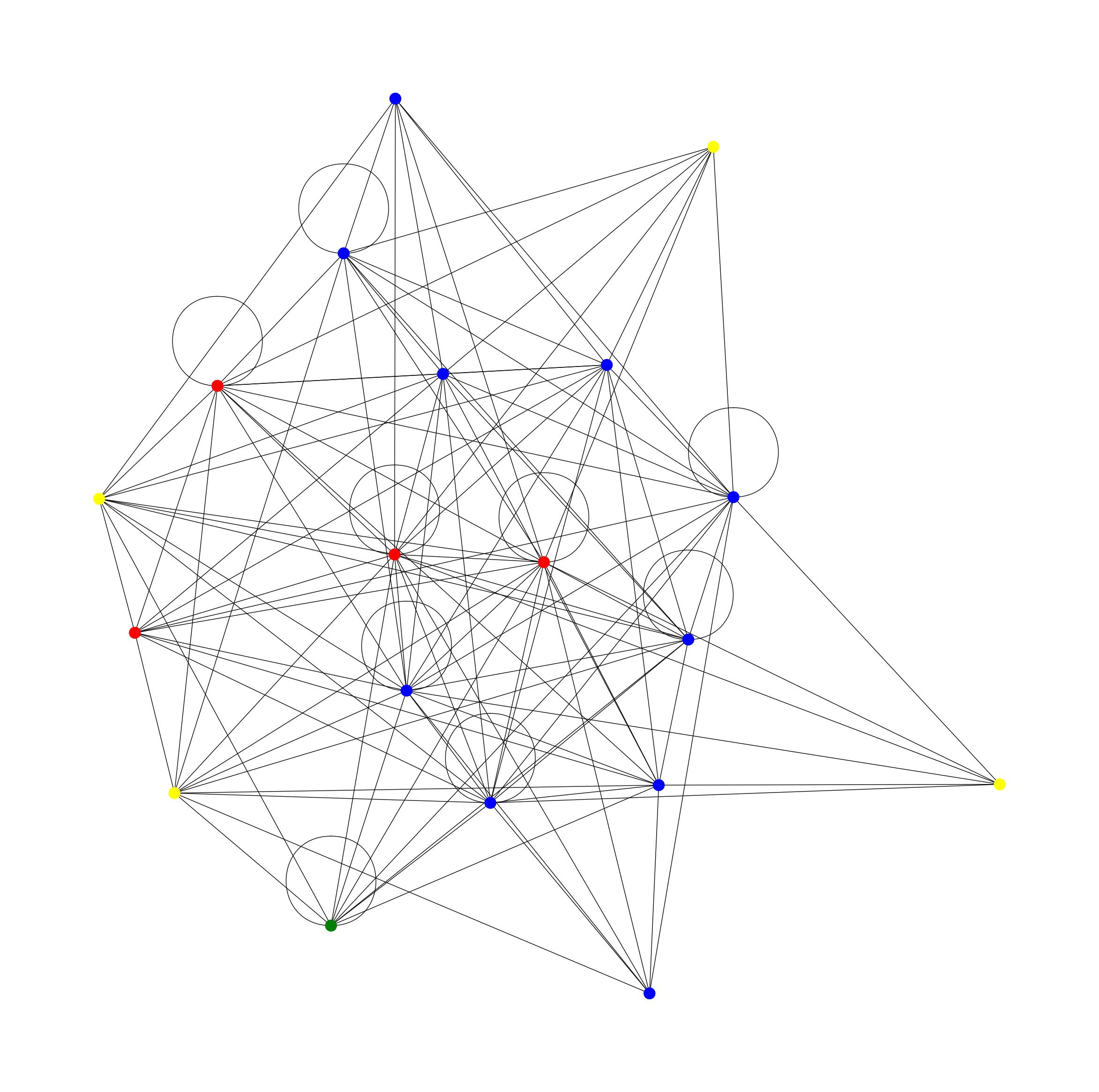
Figure 1. The graph $\mathcal{G}_{3}(2,11)$

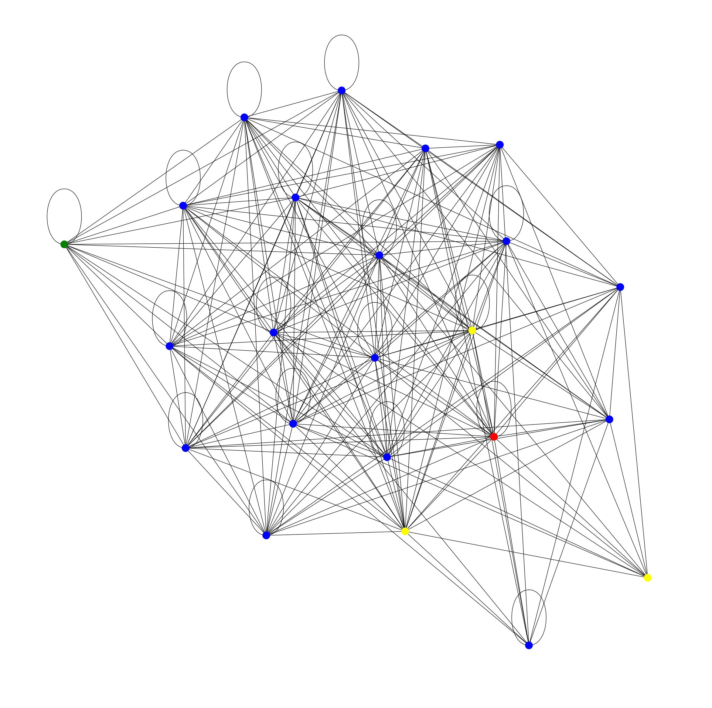
Figure 2. The graph $\mathcal{G}_{3}(2,13)$

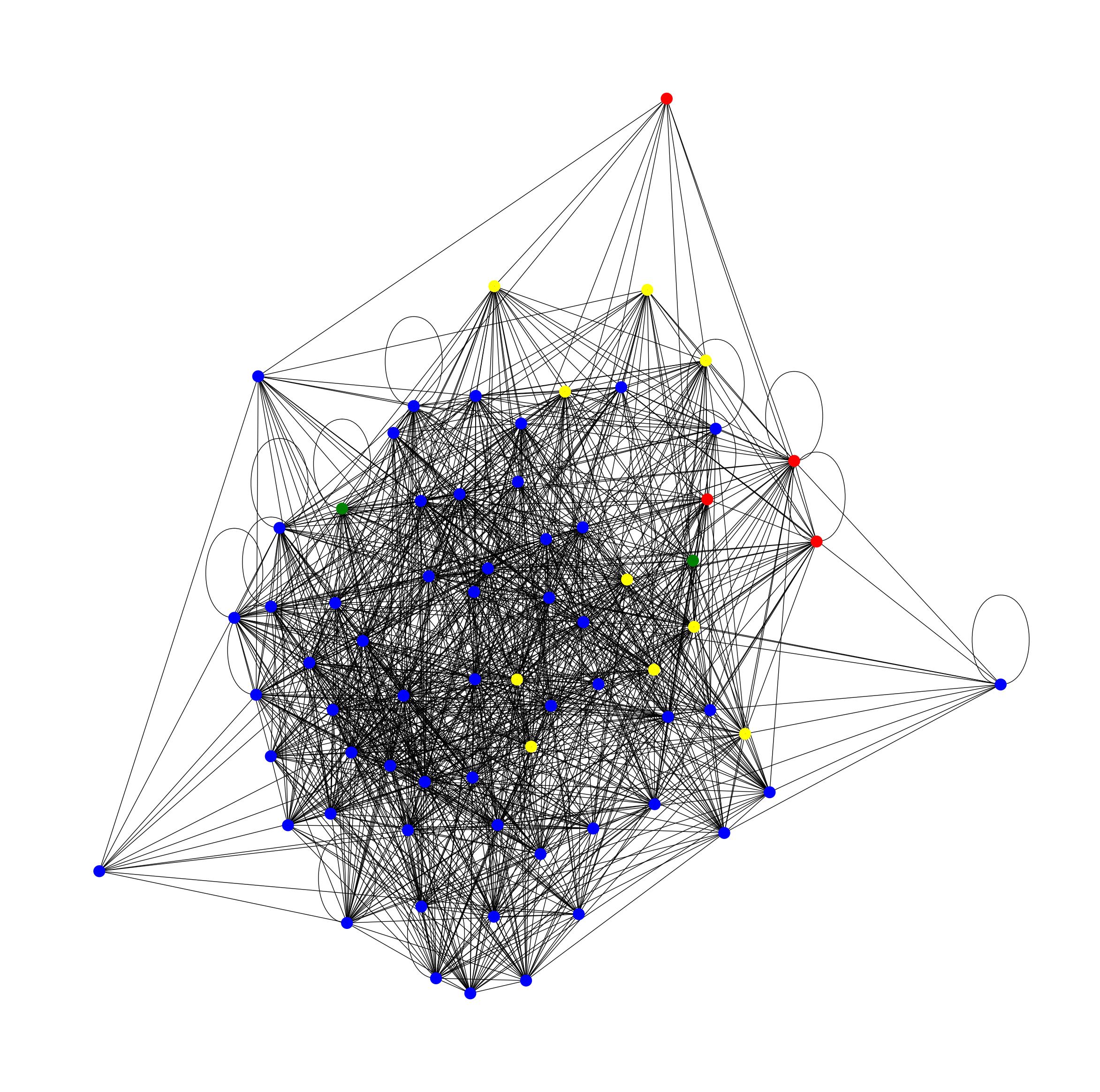
Figure 3. The graph $\mathcal{G}_{3}(2,17)$

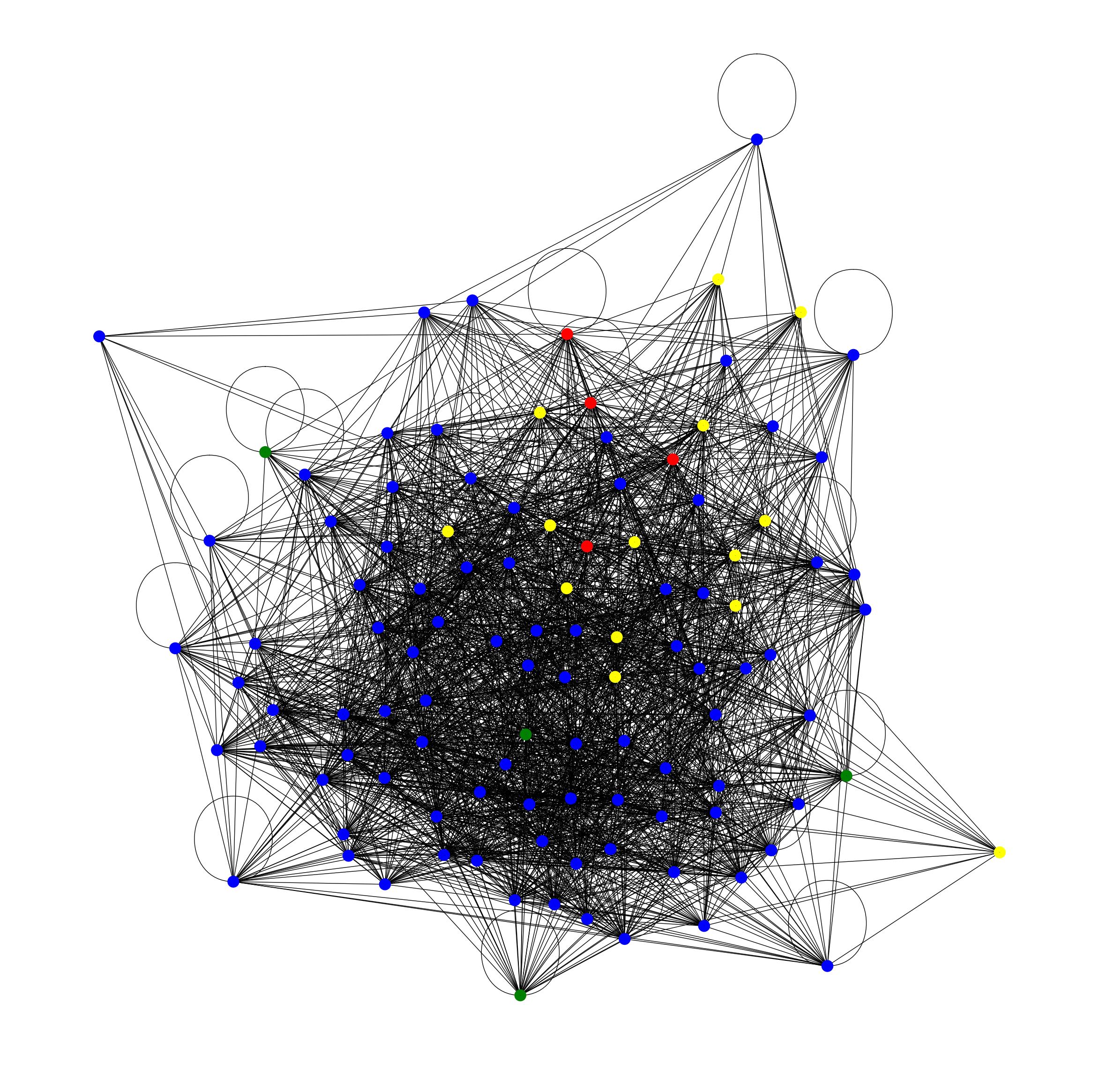
Figure 4. The graph $\mathcal{G}_{3}(2,19)$

In the above figures, we write abelian threefolds of Types $1$, $2$, $3$, and $4$ are written as blue, green, yellow, and red vertices respectively. Moreover, to improve visibility, we draw all the graphs as undirected graphs.

5. Concluding remarks

We proposed an algorithm (Algorithm 3.14) for computing the Richelot isogeny graph of superspecial abelian threefolds in characteristic $p>7$. As applications of this algorithm, we succeeded in listing up superspecial genus-3 curves for $p<100$ (Section 4.1), and finding one superspecial hyperelliptic curve of genus 3 for all $p$ with $7\leq p<10000$ (Section 4.2). Our implementation with the Magma algebraic system [2] for listing up superspecial genus-3 curves is available at

https://github.com/Ryo-Ohashi/sspg3list.

The complexity of our algorithm is estimated as $\widetilde{O}(p^{6})$ operations in the field $\mathbb{F}_{p^{2}}$ under Remark 3.17 and Assumption 3.19, but these are open problems. Therefore, theoretical proofs of them are future works.

As other future works, it would be interesting to list up superspecial curves of genus $3$ in characteristic $p>100$. However, since enumerating in $p=97$ took about a day, enumerating even in $p=199$ can be expected to take more than two months. Hence, improving the algorithm in Section 4.1 is an important task. This requires an efficient search to obtain new nodes on the graph $\mathcal{G}_{3}(2,p)$, and then we need to investigate the structure of $\mathcal{G}_{3}(2,p)$ in detail.

On the other hand, we can expect from the results in Table 1 that

Expectation 5.1.

The number of isomorphism classes of superspecial hyperelliptic curves of genus $3$ in characteristic $p$ is $O(p^{4})$.

Under this expectation, the complexity of Algorithm 4.4 can be estimated as $\widetilde{O}(p^{2})$ operations in the field $\mathbb{F}_{p^{2}}$. A theoretical proof of the above expectation is also one of our future works.

Ryo Ohashi: Graduate School of Information Science and Technology, The University of Tokyo — 7-3-1 Hongo, Bunkyo-ku, Tokyo, 113-0033, Japan.

E-mail address: ryo-ohashi@g.ecc.u-tokyo.ac.jp.

Hiroshi Onuki: Graduate School of Information Science and Technology, The University of Tokyo — 7-3-1 Hongo, Bunkyo-ku, Tokyo, 113-0033, Japan.

E-mail address: hiroshi-onuki@g.ecc.u-tokyo.ac.jp.

Momonari Kudo: Fukuoka Institute of Technology — 3-30-1 Wajiro-higashi, Higashi-ku, Fukuoka, 811-0295, Japan.

E-mail address: m-kudo@fit.ac.jp.

Ryo Yoshizumi: Joint Graduate Program of Mathematics for Innovation, Kyushu University — 744 Motooka, Nishi-ku, Fukuoka 819-0395, Japan.

E-mail address: yoshizumi.ryo.483@s.kyushu-u.ac.jp.

Koji Nuida: Institute of Mathematics for Industry, Kyushu university — 744 Motooka, Nishi-ku, Fukuoka 819-0395, Japan / National Institute of Advanced Industrial Science and Technology (AIST) — 2-3-26 Aomi, Koto-ku, Tokyo, 135-0064, Japan.

E-mail address: nuida@imi.kyushu-u.ac.jp.

References

• [1] A. Basso, L. Maino and G. Pope: FESTA: Fast encryption from supersingular torsion attacks, Asiacrypt 2023, LNCS 14444, 98–126, 2023.
• [2] W. Basso, J. Cannon and C. Playoust: The MAGMA algebra system. I. The user language, Journal of Symbolic Computation 24, 235–265, 1997.
• [3] B. W. Brock: Superspecial curves of genera two and three, Ph.D. thesis, Princeton University, 1993.
• [4] W. Castryck and T. Decru: Multiradical isogenies, preprint, https://ia.cr/2021/1133.
• [5] W. Castryck, T. Decru and B. Smith: Hash functions from superspecial genus-2 curves using Richelot isogenies, J. Math. Cryptol. 14, 268–292, 2020.
• [6] R. CossetApplications des fonctions thêta à la cryptographie sur courbes hyperelliptiques, Ph.D. thesis, Université Henri Poincaré, 2011.
• [7] R. Cosset and D. Robert: Computing $(\ell,\ell)$-isogneies in polynomial time on Jacobians of genus 2 curves, Math. Comput. 84, 1953–1975, 2014.
• [8] C. Costello and B. Smith: The supersingular isogeny problem in genus 2 and beyond, PQCrypto 2020, LNCS 12100, 151–168, 2020.
• [9] P. Dartois, A. Leroux, D. Robert and B. Wesolowski: SQISignHD: New dimensions in cryptography, preprint, https://ia.cr/2023/436.
• [10] P. Dartois, L. Maino, G. Pope, and D. Robert: An algorithmic approach to $(2,2)$-isogenies in the theta model and applications to isogeny-based cryptography, preprint, https://ia.cr/2023/1747.
• [11] M. Deuring: Die Typen der Multiplikatorenringe elliptischer Funktionenkörper, Abh. Math. Sem. Univ. Hamburg 14 (1), 197–272, 1941.
• [12] J. Dixmier: On the projective invariants of quartic plane curves, Adv. Math. 64, 279–304, 1987.
• [13] A. Fiorentino: Weber’s formula for the bitangents of a smooth plane quartic, Publ. Math. Besançon, Algèbre Théor. Nombres 2019 (2), 5–17, 2019.
• [14] E. Florit and B. Smith: Automorphisms and isogeny graphs of abelian varieties, with applications to the superspecial Richelot isogeny graph, Contemp. Math. 779, 103-132, 2022.
• [15] E. Florit and B. SmithAn atlas of the Richelot isogeny graph, RIMS Kôkyûroku Bessatsu B90, 195–219, 2022.
• [16] E. V. Flynn and Y. B. Ti: Genus two isogeny cryptography, PQCrypto 2019, LNCS 11505, 286–306, 2019.
• [17] P. Gaudry: Fast genus 2 arithmetic based on Theta functions, J. Math. Crypt. 1, 243–265, 2007.
• [18] J. P. Grass: Theta constants of genus three, Compositio Math. 40, 123–137, 1980.
• [19] E. W. Howe, F. Leprévost and B. Poonen: Large torsion subgroups of split Jacobians of curves of genus two or three, Forum Math. 12, 315–364, 2000.
• [20] T. Ibukiyama: On rational points of curves of genus 3 over finite fields, Tohoku Math. J. 45, 311–329, 1993.
• [21] T. Ibukiyama, T. Katsura and F. Oort: Supersingular curves of genus two and class numbers, Compositio Math. 57 (2), 127–152, 1986.
• [22] J. IgusaArithmetic variety of moduli for genus two, Ann. Math. 72(2), 612–649, 1960.
• [23] J. IgusaTheta functions, Grundlehren der mathematischen Wissenschaften 194, Springer–Verlag, 1972.
• [24] B. W. Jordan and Y. ZaytmanIsogeny graphs of superspecial abelian varieties and generalized Brandt matrices, preprint, arXiv: 2005.09031.
• [25] M. Kudo, S. Harashita and E. W. Howe: Algorithms to enumerate superspecial Howe curves of genus 4, The Open Book Series 4 (1), 301–316, 2020.
• [26] S. Karati and P. Sarkar: Kummer for genus one over prime-order fields, J. Cryptology 33, 97–129, 2020.
• [27] T. Katsura and K. Takashima: Counting Richelot isogenies between superspecial abelian surfaces, The Open Book Series 4 (1), 283–300, 2020. Home Selected Areas in Cryptography Conference paper
• [28] H. Lange and Ch. Birkenhake:  Complex Abelian Varieties,  Grundlehren der mathematischen Wissenschaften 302, Springer–Verlag, 2004.
• [29] R. Lercier, Q. Liu, E. L. García, C. Ritzenthaler: Reduction type of smooth quartics, Algebra Number Theory 15 (6), 1429–1468, 2021.
• [30] E. Milio: Computing isogenies between Jacobians of curves of genus 2 and 3, preprint, arXiv: 1709.06063.
• [31] D. Mumford: On the equations defining abelian varieties. I, Invent. math. 1, 287–354, 1966.
• [32] D. MumfordTata Lectures on Theta II, Progress in Mathematics 43, Birkhäuser, 1984.
• [33] T. Ohno: The graded ring of invariants of ternary quartics I, 2007, unpublished.
• [34] F. Oort: Hyperelliptic supersingular curves, Prog. Math. 89, 247–284, 1991.
• [35] E. Oyono: Non-hyperelliptic modular Jacobians of dimension 3, Math. Comput. 78, No. 266, 1173–1191, 2009.
• [36] T. Shaska and G. S. Wijesiri: Theta functions and algebraic curves with automorphisms, New Challenges in digital communications, NATO Advanced Study Institute, 193–237, 2009.
• [37] T. Shioda: On the graded ring of invariants of binary octavics, Amer. J. Math. 89, 1022–1046, 1967.
• [38] B. Smith: Explicit endomorphisms and correspondences, Ph.D. thesis, University of Sydney, 2005.
• [39] K. Takase: A generalization of Rosenhain’s normal form for hyperelliptic curves with an application, Proc. Japan Acad. 72, Ser. A, 162–165, 1996.
• [40] R. C. Valentini: Hyperelliptic curves with zero Hasse-Witt matrix, Manuscripta Math. 86, 185–194, 1995.
• [41] H. Weber: Theorie der Abelschen Functionen vom Geschlecht drei, Berlin: Druck und Verlag von Georg Reimer, 1876.