Scaling Relations of Spectrum Form Factor and Krylov Complexity at Finite Temperature

Abstract

In the study of quantum chaos diagnostics, considerable attention has been attributed to the Krylov complexity and spectrum form factor (SFF) for systems at infinite temperature. These investigations have unveiled universal properties of quantum chaotic systems. By extending the analysis to include the finite temperature effects on the Krylov complexity and SFF, we demonstrate that the Lanczos coefficients $b_{n}$, which are associated with the Wightman inner product, display consistency with the universal hypothesis presented in PRX 9, 041017 (2019). This result contrasts with the behavior of Lanczos coefficients associated with the standard inner product. Our results indicate that the slope $\alpha$ of the $b_{n}$ is bounded by $\pi k_{B}T$, where $k_{B}$ is the Boltzmann constant and $T$ the temperature. We also investigate the SFF, which characterizes the two-point correlation of the spectrum and encapsulates an indicator of ergodicity denoted by $g$ in chaotic systems. Our analysis demonstrates that as the temperature decreases, the value of $g$ decreases as well. Considering that $\alpha$ also represents the operator growth rate, we establish a quantitative relationship between ergodicity indicator and Lanczos coefficients slope. To support our findings, we provide evidence using the Gaussian orthogonal ensemble and a random spin model. Our work deepens the understanding of the finite temperature effects on Krylov complexity, SFF, and the connection between ergodicity and operator growth.

I introduction

Unveiling the scaling relations of physical quantities is an important and fundamental topic in the study of classical and quantum physics Stanley (1999); Huckestein (1995); Osterloh et al. (2002); García-García and Wang (2008); Serra et al. (1998); Pal and Huse (2010); Fisher and Berker (1982). In the context of equilibrium systems, significant progress has been made in this direction, leading to a deeper understanding of critical phenomena, phase transitions, and universal behaviors Hung et al. (2011); Puebla et al. (2019); Chen et al. (2019); Chauhan et al. (2022). The investigation of scaling relations in numerous systems are still attracting a growing interests, especially in the context of non-equilibrium systems and quantum dynamics of chaotic systems Sierant et al. (2020); Šuntajs et al. (2020).

Quantum chaos has been an attractive topic across diverse disciplines, spanning from condensed matter physics to black hole physics and high-energy physics Cotler et al. (2017a); García-García and Verbaarschot (2016); Cotler et al. (2017b). This field holds the potential to offer deeper insights into phenomena like thermalization Deutsch (2018, 1991); Srednicki (1994); Rigol et al. (2008); Kim et al. (2014); Abanin et al. (2019), information scrambling Yan et al. (2020); Shen et al. (2020); et al. (2021); Landsman et al. (2019), and quantum entanglement Abanin et al. (2019); Žnidarič et al. (2008); Bardarson et al. (2012). However, comprehensively diagnosing quantum chaos remains a formidable challenge. To date, several methods have emerged for characterizing the nature of quantum chaos. These include spectrum statistics Shklovskii et al. (1993); Frisch et al. (2014); Liu (2018), out-of-time-correlation von Keyserlingk et al. (2018); Rakovszky et al. (2018), Loschmidt echo Yan et al. (2020), and complexity Prosen (2007). Each diagnostic tool captures different aspects of quantum chaos and provides valuable insights individually. Recently, spectrum form factor (SFF) Cotler et al. (2017a, b); Gharibyan et al. (2018); Chen and Ludwig (2018); Chan et al. (2018a) and Krylov complexity (K-complexity)  Parker et al. (2019) stand out as prominent examples, offering perceptions into the energy spectrum and operator growth in quantum chaotic systems.

Typically, the characteristics of quantum chaos manifest across the entire spectrum. To quantify the chaos strength, the statistical properties are conventionally studied. For example, the Wigner-Dyson distribution describes the statistical properties of a quantum chaotic system at infinite temperature, where a level repulsion presents in the energy spectrum Guhr et al. (1998); Mehta (1991); Haake (2010). The statistical properties of the spectrum provide information solely about the nearest level spacing within the spectrum. In contrast, the SFF measures energy correlations between any two states, which allows it to go beyond the constraints of spectrum statistics and capture richer information. SFF has found widespread use in diverse contexts, including random matrix theory (RMT) Guhr et al. (1998); Brody et al. (1981); Mehta (1991); Haake (2010); Kos et al. (2018), the Sachdev-Ye-Kitaev model Cotler et al. (2017b, a), and the Hubbard model Zhou et al. (2023); Wittmann W. et al. (2022); Dağ et al. (2023). The intriguing dip-ramp-plateau structure observed in many chaotic systems indicats the universality of SFF Gharibyan et al. (2018); Saad et al. (2019); Winer et al. (2020). The SFF can also be generalized to encapsulate the correlation between multi energy levels Liu (2018); Wei et al. (2024); Cardella (2021); Gross and Rosenhaus (2017).

In quantum systems, the chaotic feature can also be manifested through operator growth. Specifically, the evolution of an initially simple operator $\hat{\cal O}(0)$ gradually becomes more complex under the Heisenberg evolution. This occurs because the operator $\hat{\cal O}(0)$ does not commute with the Hamiltonian $\hat{H}$ of an interacting quantum system. Several approaches have been proposed to quantify the operator growth Nahum et al. (2018); Khemani et al. (2018); Chan et al. (2018b); Roberts et al. (2018). Recently, the concept of K-complexity was introduced to characterize operator growth Parker et al. (2019) and has been applied to various systems, including strongly correlated systems, quantum circuits, and black hole physics Barbón et al. (2020); Magán and Simón (2020); Jian et al. (2021); Kar et al. (2022); Liu et al. (2022); Barbón et al. (2019); Dymarsky and Gorsky (2020); Xu et al. (2020); Avdoshkin and Dymarsky (2020); Rabinovici et al. (2021); Dymarsky and Smolkin (2021); Trigueros and Lin (2022); Kim et al. (2022); Hörnedal et al. (2022); Rabinovici et al. (2022a); Bhattacharjee et al. (2022); Balasubramanian et al. (2022); Heveling et al. (2022); Adhikari and Choudhury (2022); Adhikari et al. (2022); Caputa and Liu (2022); Mück and Yang (2022); Banerjee et al. (2022); Fan (2022a, b); Rabinovici et al. (2022b); Bhattacharyya et al. (2023). It was found that operator growth can be quantified by the mean value of wave packet position on a half-infinite chain. Motivated by this idea, a universal hypothesis of operator growth has also been proposed, where the Lanczos coefficients can be used to diagnose the presence of quantum chaos. Meanwhile, the autocorrelation function ${\cal C}(t)={\rm Tr}(\hat{\cal O}(t)\hat{\cal O}(0))$ defined at infinite temperature can be readily obtained and has been intensively studied in various contexts Kubo (1957); Alhambra et al. (2020); Carabba et al. (2022). It is surprising to find that the universal behavior of the autocorrelation function is determined by the first few Lanczos coefficients Zhang and Zhai (2023). In addition, some studies have explored the relations between K-complexity and other complexity measures, such as circuit complexity, leading to a geometric interpretation of K-complexity Caputa et al. (2022); Lv et al. (2023); Hörnedal et al. (2023).

In this work, we establish a connection between K-complexity and SFF at finite temperature. Our main conclusions can be summarized as follows: (1) The use of the Wightman inner product and the standard inner product results in distinct Lanczos coefficients $b_{n}$, and the slope $\alpha$ of $b_{n}$ in the former is limited by $\pi k_{B}T$; (2) The ergodicity indicator $g$ diminishes with decreasing temperature; (3) We establish a quantitative relationship between $g$ and $\alpha$ after proper scaling.

II Lanczos coefficients at finite temperature

Let us begin with a brief review of the derivation of Lanczos coefficients, and highlight the finite temperature effect of operator growth. Consider a scenario where we have a simple operator $\hat{\cal O}$ and a Hamiltonian $\hat{H}$. Typically, in the presence of interactions, they do not commute. The evolution of the operator $\hat{\cal O}$ follows the Heisenberg equation $-i\partial_{t}\hat{\cal O}(t)=[\hat{H},\hat{\cal O}(t)]$, and the formal solution reads $\hat{\cal O}(t)={\rm e}^{i\hat{H}t}\hat{\cal O}{\rm e}^{-i\hat{H}t}$. Henceforth, we set $\hbar=1$. Therefore, the initial simple operator becomes progressively more complex due to the noncommutative relation between $\hat{\cal O}(t)$ and $\hat{H}$, which is also termed as operator growth. In order to quantify the complexity of $\hat{\cal O}(t)$, the concept of K-complexity was introduced by Parker, et.al. Parker et al. (2019). Given a Hilbert space spanned by ${\ket{i}}$, the operator $\hat{\cal O}=\sum_{i,j}{\cal O}_{ij}\ket{i}\bra{j}$ can be mapped to an “operator state” $|{\hat{\cal O}}\rangle=\sum_{i,j}{\cal O}_{ij}\ket{i}\otimes\ket{j}$ living in the double Hilbert space spanned by ${\ket{i}\otimes\ket{j}}$. By defining a Liouvillian superoperator $\hat{\cal L}=[\hat{H},\cdots]$, the Heisenberg equation can be rewritten as $\partial_{t}|{\hat{\cal O}(t)}\rangle=i\hat{\cal L}|{\hat{\cal O}(t)}\rangle$. In the double Hilbert space, the Liouvillian superoperator appears as a conventional operator, and can be written as $\hat{\cal L}=\hat{H}\otimes\hat{\mathbb{I}}-\hat{\mathbb{I}}\otimes\hat{H}^{T}$ where $\hat{\mathbb{I}}$ denotes the identity operator with the same dimension of $\hat{H}$. The superscript $T$ denotes transpose. The time-dependent operator state can be expressed as:

$$|\hat{\cal O}(t)\rangle={\rm e}^{i\hat{\cal L}t}|{\hat{\cal O}}\rangle=\sum_{n=0}^{\infty}\frac{(it)^{n}}{n!}|{\hat{\cal L}^{n}\hat{\cal O}}\rangle.$$ (1)

This means that $|{\hat{\cal O}(t)}\rangle$ can be expanded under the basis spanned by ${|{\hat{\cal L}^{n}\hat{\cal O}}}\rangle$. It is important to note that this basis is neither normalized nor orthogonal. To address this issue, the Krylov basis is defined by the Gram-Schmidt orthogonalization. It is pointed out that one must properly define the inner product of two operator states as follows:

$$\langle{\hat{A}}|{\hat{B}}\rangle_{\beta}^{g}=\frac{1}{Z}\int_{0}^{\infty}g(\lambda){\rm Tr}({\rm e}^{-\beta\hat{H}}{\rm e}^{\lambda\hat{H}}\hat{A}^{\dagger}{\rm e}^{-\lambda\hat{H}}\hat{B})d\lambda.$$ (2)

Here, $Z={\rm Tr}({\rm e}^{-\beta\hat{H}})$ denotes the partition function, $\beta=1/(k_{\rm B}T)$ represents the inverse temperature, and $k_{\rm B}$ indicates the Boltzmann constant. $g(\lambda)$ satisfies the conditions $g(\lambda)\geq 0$, $g(\beta-\lambda)=g(\lambda)$, and $\beta^{-1}\int_{0}^{\beta}d\lambda g(\lambda)=1$  Parker et al. (2019). Different choices of $g(\lambda)$ define distinct inner products. In this work, we consider two specific choices: (1) The standard inner product is defined by choosing $g(\lambda)=[\delta(\lambda)+\delta(\lambda-\beta)]/2$, and can be explicitly written as:

$$\langle{\hat{A}}|{\hat{B}}\rangle_{\beta}^{S}=\frac{1}{2Z}{\rm Tr}\left({\rm e}^{-\beta\hat{H}}\hat{A}^{\dagger}\hat{B}+\hat{A}^{\dagger}{\rm e}^{-\beta\hat{H}}\hat{B}\right).$$ (3)

Here, by “standard” we mean that this kind of inner product is widely adopted in the linear response theory. (2) Another inner product often considered in quantum field theory is the Wightman inner product, defined by $g(\lambda)=\delta(\lambda-\beta/2)$, and can be explicitly written as:

$$\langle{\hat{A}}|{\hat{B}}\rangle_{\beta}^{W}=\frac{1}{Z}{\rm Tr}\left(e^{-\beta\hat{H}/2}\hat{A}^{\dagger}e^{\beta\hat{H}/2}\hat{B}\right).$$ (4)

It should be noted that at infinitely high temperature, i.e., $\beta\to 0$, both the standard and Wightman inner products reduce to the same one: $\langle{\hat{A}}|{\hat{B}}\rangle={\rm Tr}\left(\hat{A}^{\dagger}\hat{B}\right)/{\rm Tr}(\hat{\mathbb{I}})$. Equipped with the inner product, we can define the Krylov basis denoted by ${|{\hat{\cal O}_{n}}}\rangle$ using the Lanczos algorithm as follows: for $n=1,2$, we have $|{\hat{\cal O}_{0}}\rangle=|{\hat{\cal O}}\rangle$ and $|{\hat{\cal O}_{1}}\rangle=b_{1}^{-1}\hat{\cal L}|{\hat{\cal O}_{0}}\rangle$, respectively, where $b_{1}=\langle{\hat{\cal L}\hat{\cal O}_{0}}|{\hat{\cal L}\hat{\cal O}_{0}}\rangle^{1/2}$; then for $n>2$, $|{\hat{\cal O}_{n}}\rangle$ can be defined inductively as:

$$|{\hat{\cal A}_{n}}\rangle= \hat{\cal L}|{\hat{\cal O}_{n-1}}\rangle-b_{n-1}|{\hat{\cal O}_{n-2}}\rangle;$$

$$b_{n}= \left[\langle{\hat{\cal A}_{n}}|{\hat{\cal A}_{n}}\rangle_{\beta}^{g}\right]^{1/2};$$ (5)

$$|{\hat{\cal O}_{n}}\rangle= b_{n}^{-1}|{\hat{\cal A}_{n}}\rangle.$$

Here, $b_{n}$’s indicate the Lanczos coefficients, which obviously depends on temperature. Previous research has demonstrated that the asymptotic behavior of these coefficients at large $n$ can be utilized as a diagnostic for chaotic systems Parker et al. (2019). Using the completeness and orthogonality of the Krylov basis, the Heisenberg equation can be mapped to a discrete Schrödinger-like equation $\partial_{t}\varphi_{n}(t)=b_{n}\varphi_{n-1}(t)-b_{n+1}\varphi_{n+1}(t)$ with $\varphi_{n}(t)=i^{-n}\langle{\cal O}_{n}|{\cal O}(t)\rangle$. The natural initial condition reads $\varphi_{n}(0)=\delta_{n0}$.

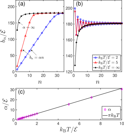
Figure 1: Finite temperature Lanczos coefficients $b_{n}$ for Gaussian orthogonal ensemble (GOE). The operator is chosen as $\hat{\sigma}_{z}\otimes\hat{\mathbb{I}}_{L/2}$, and the dimension of random matrix is $8192$. In (a) and (b), Wightman and standard inner product are used, respectively. (a): At finite temperature, $\{b_{n}\}$ defined by Wightman inner product shows linear behavior, which is consistent with the universal hypothesis. (b): The finite temperature $b_{n}$ presents oscillatory behavior which is in contrast to the universal hypothesis. (c): The slope $\alpha(T)=\pi k_{\rm B}T$ aligns with upper bound of the operator growth rate, and approach at infinite temperature.

To illustrate the difference in ${b_{n}}$’s defined by the standard and Wightman inner products, we calculate ${b_{n}}$ for the Gaussian orthogonal ensemble (GOE), which serves as an ideal chaotic model. The Hamiltonian can be expressed as $\hat{H}_{\rm GOE}=\mathcal{E}{\rm GOE}(L,\mu,\sigma)$, where the $\mathcal{E}$ is the characteristic energy and ${\rm GOE}(L,\mu,\sigma)$ represents a $L\times L$ Hermitian matrix of which the elements are sampled from Gaussian distribution with mean value $\mu$ and standard deviation $\sigma$. The operator is chosen as $\hat{\sigma}_{z}\otimes\hat{\mathbb{I}}_{L/2}$, where $\hat{\sigma}_{z}$ and $\hat{\mathbb{I}}_{L/2}$ denote the Pauli matrix and $L/2\times L/2$ identity matrix, respectively. Obviously, this is a simple operator. By simple, we mean it is represented by a sparse matrix. In evolution, this operator becomes complex progressively. The ${b_{n}}$’s obtained using the Wightman and standard inner products are shown in Fig. 1(a) and (b), respectively. It is important to note that at infinite temperature, both inner products yield the same ${b_{n}}$ values, aligning with our expectations. However, the $b_{n}$’s at finite temperature showcase quite different behaviors for the above-mentioned inner products. The Wightman inner product leads to a linear $b_{n}$ at small $n$, i.e., $b_{n}\approx\alpha(T)n$. The slope $\alpha$ increases as the temperature rises and approaches infinity at infinite temperature. This is reasonable in the sense that at higher temperatures, the speed of operator growth is larger. The range of $n$ that supports linear $b_{n}$ also extends at low temperatures. This indicates that the universal hypothesis is applicable even at finite temperature when the Wightman inner product is adopted. The saturation at large $n$ is due to finite-size effects. In contrast, $b_{n}$ shows oscillatory behavior at finite temperature when the standard inner product is used, and the oscillatory behavior becomes more pronounced at lower temperatures, which is not aligned with the universal hypothesis. In the following analysis, we will focus on the Wightman inner product. In Fig. 1(c), we present the slope $\alpha(T)$ for various temperatures. It is clear that for GOE,

$$\alpha(T)=\pi k_{B}T,$$ (6)

which, on one hand, is consistent with the universal hypothesis on the upper bound of the Lanczos coefficient growth rate $\alpha(T)\leq\pi k_{B}T$, and on the other hand, manifests GOE being the most chaotic model. The slight derivation at high temperature is due to the finite size effect.

III Spectrum form factor

The SFF is another emerging diagnostic of quantum chaosCotler et al. (2017b); Kos et al. (2018), which measures the spectrum correlation of arbitrary two states. Specifically, we consider the following spectrum correlation,

$${\cal C}(E)=\frac{1}{L^{2}}\sum_{i,j}\delta\left[E-\left(E_{i}-E_{j}\right)\right],$$ (7)

It is evident that as long as the energy difference between two states is $E$, they contribute to ${\cal C}(E)$, regardless of whether they are the nearest neighbors or not. The SFF can be obtained by a Fourier transform as follows:

$$K(t)=L\int dEe^{-iEt}{\cal C}(E)=\frac{1}{L}\left|{\rm Tr}\left({\rm e}^{-i\hat{H}t}\right)\right|^{2}.$$ (8)

It has been demonstrated that the “dip-ramp-plateau” structure of SFF is a universal behavior for quantum chaotic systems. In the long time limit, $K(t)\to 1$ according to our definition. Moreover, the SFF can also be generalized to finite temperature by the analytical extension $t\to t-i\beta$, where $\beta=1/(k_{B}T)$ Cotler et al. (2017b). The finite temperature effect of SFF has been investigated in paradigmatic quantum chaotic systems, and the “dip-ramp-plateau” structure survives, which is reproduced in Fig. 2.

Two time scales can be extracted from the SFF Edwards and Thouless (1972); Thouless (1974); Sierant et al. (2020); Šuntajs et al. (2020); one is the Heisenberg time $t_{\rm H}$; the other one is the Thouless time $t_{\rm Th}$. The former one is defined as $t_{\rm H}=2\pi/\Delta$ with $\Delta$ being the mean energy level spacing which exponentially decreases as the system size increases Sierant et al. (2020); Šuntajs et al. (2020). In SFF, the Heisenberg time can be pinned down by the presence of plateau. The Thouless time is the timescale that characterizes how initial local information diffuses throughout the system, and can be defined as the timescale beyond which the SFF becomes consistent the universal one of GOE. In contrast to the Heisenberg time, the Thouless time increases polynomially as the system time increases Sierant et al. (2020); Šuntajs et al. (2020); D’Alessio et al. (2016). In RMT, the analytical form of $K(t)$ at infinite temperature is available. For instance, $K(t)$ of GOE at intermediate and long time can be written as Vasilyev et al. (2020)

$$K_{\rm a}(t)=\left\{\begin{aligned} &\frac{2t}{t_{\rm H}}-\frac{t}{t_{\rm H}}{\rm log}_{10}\left(1+\frac{2t}{t_{\rm H}}\right),0<t<t_{\rm H}\\ &2-\frac{t}{t_{\rm H}}{\rm log}_{10}\left(\frac{2t+t_{\rm H}}{2t-t_{\rm H}}\right),t>t_{\rm H}\end{aligned}\right.,$$ (9)

where we have taken the random average with respect to the probability of GOE. It can be checked that in the long time limit $K_{\rm a}(t)\to 1$, which is consistent with our definition in Eq.(8).

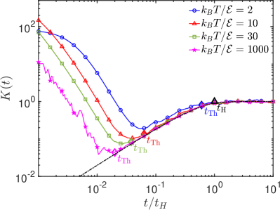
Figure 2: The spectrum form factor(SFF) at finite temperature. The “dip-ramp-plateau” structure of SFF survives at finite temperature(colored line). The Thouless time(colored diamond) is determined as SFF at finite temperature is close enough to the analytical SFF(black dash line) of GOE at infinite temperature. The Heisenberg time is shown as the black triangle marker.

With the Heisenberg and Thouless time, a quantity to measure the ergodicity in quantum systems is defined,

$$g=\log_{10}(t_{\rm H}/t_{\rm Th})$$ (10)

which is termed as ergodicity indicator Sierant et al. (2020); Šuntajs et al. (2020). In the thermodynamic limit, the ergodicity indicator $g$ describes a transition from the quantum ergodic regime $g\to\infty$ ($t_{\rm H}/t_{\rm Th}\to\infty$) to nonergodic regime $g\to-\infty$ ($t_{\rm H}/t_{\rm Th}\to 0$).

Similar to the generalization of SFF, we extend the ergodicity indicator to finite temperature since the Heisenberg and Thouless time can still be extracted from the SFF at finite temperature. In Fig. 2, we illustrate the extraction of Heisenberg and Thouless time from SFF at finite temperature. Specifically, we numerically generate 150 samples of GOE at system size of $L=4096$ for each considered temperature. Following the method in Sierant et al. (2020); Šuntajs et al. (2020), we apply the unfolding procedure, which maps each eigenvalue $E_{i}$ to a dimensionless number $\epsilon_{i}$ times average level spacing $\Delta$ and avoids the global energy dependence. Meanwhile, the information in local energy fluctuation reserves Haake (2010). Then the SFF after the unfolding procedure is written as

$$K(t)=\frac{1}{L}\left|\sum_{i}{\rm e}^{-iE_{i}t}\right|^{2}\to \frac{1}{L}\left|\sum_{i}{\rm e}^{-i(\epsilon_{i}\Delta)t}\right|^{2}$$

$$= \frac{1}{L}\left|\sum_{i}{\rm e}^{-i2\pi\epsilon_{i}t/t_{\rm H}}\right|^{2}.$$ (11)

In the last step, we use the definition of the Heisenberg time $t_{\rm H}=2\pi/\Delta$. Therefore, the Heisenberg time, labelled by the black triangle in Fig. 2, naturally serves as the time unit. The colored solid lines represent the average SFF of 150 samples in GOE at various temperature. It is evident that the SFF at finite temperature adheres to the analytical SFF $K_{\rm a}(t)$(black dash line) after the Thouless time(colored diamond). Numerically, the Thouless time is determined when finite temperature SFFs are sufficiently close to analytical SFF $K_{\rm a}(t)$, the quantitative criterion of which reads $\left|{\rm log}_{10}\left[\frac{K(t_{\rm Th})}{K_{\rm a}(t_{\rm Th})}\right]\right|<0.05$ Sierant et al. (2020). It is evident that a system with lower temperature exhibits a longer Thouless time, resulting in a smaller ergodicity indicator. This observation aligns with our intuition, indicating that the reduction in temperature suppresses the characteristics of chaos, as similarly observed in the previous section for Lanczos coefficients.

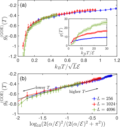
Figure 3: The scaled ergodicity indicator $g^{\rm(GOE)}_{S}(T)$ and its relation to the slope $\alpha(T)$ of Lanczos coefficients. (a): The initial ergodicity indicators displayed in the inset are different by a size dependence. After scaling, the scaled ergodicity indicators of different system size show collapse to a single curve. (b): The linear relation between scaled ergodicity indicator and Lanczos coefficients slope. The error bar of scaled ergodicity indicator is the standard deviation of 10 sets of samples. The fluctuation of $\alpha(T)$ is so small during the sampling procedure that the error bar on Krylov complexity side is not shown. The black dotted line is plotted to show linearity.

IV Scaling relation of GOE

As of now, we present two chaos diagnostic tools that depend on temperature. A natural question arises: what is the relation between them? In this section, we present a scaling relationship between the ergodicity indicator $g(T)$ and the slope of Lanczos coefficients $\alpha(T)$ at different temperature, which is showcased in Fig. 3(b). To this end, we firstly study the temperature dependence of ergodicity indicator $g(T)$, as illustrated in the inset of Fig. 3(a). The ergodicity indicator increases as the temperature ramps, as expected, and it also shows size dependency, the same as SFF Cotler et al. (2017b). This size dependence precludes a meaningful and direct quantitative comparison between $g(T)$ and $\alpha(T)$.

In order to eliminate the size-dependent effects, a scaled ergodicity indicator denoted as $g^{\rm(GOE)}_{\rm S}(T)$ has been proposed. It remains invariant with respect to different system size. Notably, for a particular system that can be simulated by GOE, the spectrum spans approximately from $-\mathcal{E}\sqrt{L}$ to $\mathcal{E}\sqrt{L}$. We postulate that temperature should be scaled by a factor of $\sqrt{L}$. Using the definition of Heisenberg time, we find that it is system size-dependent, i.e., $t_{\rm H}=2\pi L/(E_{\rm max}-E_{\rm min})\sim 2\pi\sqrt{L}/\mathcal{E}$. This contrasts with the Thouless time. As such, we can shift the value of the ergodicity indicator by amount of $\log_{10}(\sqrt{L})$, and define scaled ergodicity indicator as

$$g^{\rm(GOE)}_{\rm S}(T)={\rm log}_{10}\left[\frac{t_{\rm H}}{t_{\rm Th}(T)\sqrt{L}}\right].$$ (12)

In Fig. 3(a), we present the scaled ergodicity indicator for different system size. Our results show that, within a broad temperature range, the scaled ergodicity indicators, denoted as $g^{\rm(GOE)}_{\rm S}(T)$, collapse to a single curve across various system sizes. We also would like to mention that the temperature in Fig. 3(a) has also be scaled by $\sqrt{L}$, which confirms our previous postulation. The error bars represent the standard deviations of scaled ergodicity indicators from ten repetitions of sampling procedure.

Then the relation between $g^{\rm(GOE)}_{\rm S}(T)$ and $\alpha(T)$ can be well defined. It has been demonstrated that the ratio of the time it takes for the SFF to reach the minimum and the plateau is proportional to $\sqrt{L}/(1+\beta^{2}/2)$ for GUE Cotler et al. (2017b). Noticing that the SFF at Thouless time is close to the minimum and the Heisenberg time is pinned down by the presence of plateau, we conjecture the ratio of Heisenberg time and Thouless time for GOE has similar form and can be written as

$$\frac{t_{\rm H}}{t_{\rm Th}}\propto\left(\frac{\sqrt{L}}{1+\beta^{2}\mathcal{E}^{2}/2}\right)^{\delta}.$$ (13)

Here, $\delta$ is a fitting parameter and $\beta\mathcal{E}$ is dimensionless. Upon substituting Eq.(13) and (6) into Eq.(12), we obtain a scaling relation between $g^{\rm(GOE)}_{\rm S}(T)$ and $\alpha(T)$,

$$g^{\rm(GOE)}_{\rm S}(T)=\delta{\rm log}_{10}\left[\frac{2(\alpha(T)/\mathcal{E})^{2}}{2(\alpha(T)/\mathcal{E})^{2}+\pi^{2}}\right]+C,$$ (14)

where we have used $\beta=1/k_{\rm B}T$ and $C$ is a fitting parameter. In Fig. 3(b), we show that Eq.(14) indeed holds. For different system sizes, the curves collapse to a single one. By fitting Eq.(14) to numerical results, we find $\delta=0.25$ and $C=-0.21$. The origin of the error bars is the same as that for scaled ergodicity indicators.

V Scaling relation of random spin model

Up to now, we work on the random matrices which describe sufficient complicated and chaotic systems. In this section, we study a 1D Ising model in transverse and longitudinal field, TL-Ising model in short. In our calculation, the longitudinal field takes a random value on each site. This model is nonintegrable and chaotic at uniform transverse and random longitudinal field Noh (2021); Nivedita et al. (2020); Trigueros and Lin (2022). And the energy spectrum follows the Wigner-Dyson distribution, which is a hallmark of quantum chaos. Besides, we choose the random parameter far away from the many-body-localization phase Trigueros and Lin (2022); De Tomasi et al. (2021) to reserve the chaotic characteristics. In this system, the linear scaling relation is tested.

Specifically, the Hamiltonian of TL-Ising model is written as

$$\hat{H}_{\rm spin}=\sum_{i}^{N}(-J\hat{\sigma}^{x}_{i}\hat{\sigma}^{x}_{i+1}+h\hat{\sigma}^{z}_{i}+g_{i}\hat{\sigma}^{x}_{i}),$$ (15)

where $J$ is the near-neighbor coupling and taken as the energy dimension in the following discussion, $h$ represents the uniform transverse field and $g_{i}$ represents the site-dependent longitudinal field, $N$ is the total number of spin and $\hat{\sigma}_{i}^{a}$ with $a=x,z$ is the Pauli operator on $i$-th site. Formally, this operator should be considered in version of direct product that $\hat{\sigma}_{i}^{a}=...\otimes\underbrace{\hat{\mathbb{I}}_{2}}_{i-1\text{-th site}}\otimes\underbrace{\hat{\sigma}^{a}}_{i\text{-th site}}\otimes\underbrace{\hat{\mathbb{I}}_{2}}_{i+1\text{-th site}}\otimes...$ with $\hat{\mathbb{I}}_{2}$ being the $2\times 2$ identity operator. When the longitudinal field is turned off ($g_{i}=0$ for each site), this model can be mapped to a free fermion model and becomes integrable. As shown in Noh (2021) with sightly applying uniform longitudinal field, the integrability is broken and the system tends to be chaotic. In our case, we take site-dependent longitudinal field $g_{i}$, which is sampled from a uniform distribution.

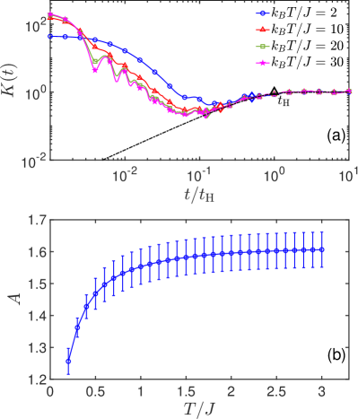
Figure 4: The SFF and logarithmic corrected slope $A(T)$ of spin model in transverse and random longitudinal field(TL-Ising model) at finite temperature. (a): The black dash line is the analytical SFF of GOE at infinite temperature. The colored solid lines represent the average SFF of TL-Ising model at finite temperature, from which the Thouless time is extracted(colored diamond). The Heisenberg time is still labelled by black triangle. (b): The slope $A(T)$ of Lanczos coefficient defined by the Wightman inner product exhibits a progressive increase with rising temperature and saturates at high temperature. The error bar is the standard deviation of 10 sets of samples.

The SFF of TL-Ising model at finite temperature is shown in Fig. 4(a), where $N=8$, $h=J$ and $g_{i}$ is sampled from $[-J,J]$. Each colored curve of SFF data is taken average from 200 samples. The “dip-ramp-plateau” structure can be observed, which confirms the existence of chaos. Using the same method illustrated in GOE, the Thouless time $t_{\rm Th}$ and Heisenberg time $t_{\rm H}$ are extracted from the SFF data. The Heisenberg time still serves as a time unit. At lower temperature, the SFF of TL-Ising model takes longer time to adhere to the analytical SFF of GOE, indicating larger Thouless time. Then the ergodicity indicator defined by Eq.(10) can be calculated. As expected, the ergodicity indicator shows a size dependence, seen in the inset of Fig. 5(a). As such, we need to scale the SFF to avoid the size effect.

The scaling method on TL-Ising model is different from the case of random matrix. For energy of TL-Ising model ranges from $\sim-JN$ to $\sim JN$. The temperature $k_{B}T/J$ is scaled to $k_{B}T/NJ$. In contrast to GOE, the Thouless time is proportion to $N^{2}$ Sierant et al. (2020); Šuntajs et al. (2020); D’Alessio et al. (2016). Therefore, the scaled ergodicity indicator for TL-Ising model is written as

$$g_{\rm S}^{\rm(Ising)}(T)={\rm log}_{10}\left[\frac{t_{\rm H}N^{2}}{t_{\rm Th}(T)}\right].$$ (16)

As shown in Fig. 5(a), the size effect on ergodicity indicator for TL-Ising model is almost eliminated.

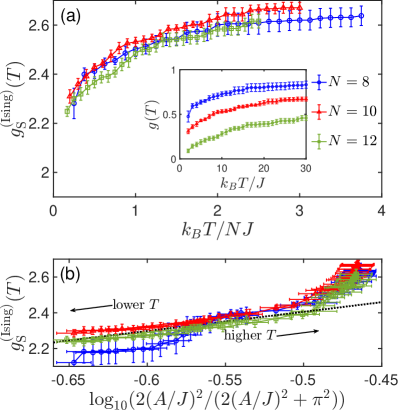
Figure 5: The scaled ergodicity indicator $g^{\rm(Ising)}_{S}(T)$ and the relation between $g^{\rm(Ising)}_{S}(T)$ and $A(T)$ for TL-Ising model. (a): The initial ergodicity indicator is displayed in the inset, which also presents system size dependence. The finite size dependence is eliminated in the scaled ergodicity indicator. (b): The relation between the scaled ergodicity indicator and $A(T)$. The linearity can be observed at relatively low temperature. The black dotted line is plotted to show linearity.

On the Krylov complexity side, we also use the Wightman inner product in the calculation of Lanczos coefficient $b_{n}$. In our calculation, the operator is chosen as $\hat{\sigma}^{(1)}_{z}\otimes\Pi_{i=2}^{N}\hat{\mathbb{I}}_{2}^{(i)}$. As the system is one dimensional, the linear growth of $b_{n}$ is corrected by logarithmic correction $b_{n}=A(T)n/{\rm ln}(n)$. Here $A(T)$ is the slope of $\left\{b_{n}\right\}$ sequence after logarithmic correction. Considering the disordered longitudinal field, we obtain the final $b_{n}$ by the mean value of 10 samples, and fit the results by a linear function. The temperature dependence of $A(T)$ is shown in Fig. 4(b). The points in figure represent the average of $A(T)$ from five repetitions and the error bars represent their standard deviations. It is obvious that $A(T)$ tends to saturate at high temperature limit, which indicates the TL-Ising model is chaotic but not sufficiently chaotic.

Then the scaling relation between the scaled ergodicity indicator and the Lanczos coefficients slope can be established. Inspired by the similarity of spectral properties between GOE and TL-Ising model Sierant et al. (2020); Šuntajs et al. (2020), we expect that the scaling law established in GOE should also hold for the TL-Ising model. Therefore, the counterpart of Eq. (14) can be written as

$$g_{\rm S}^{\rm(Ising)}(T)=\delta{\rm log}_{10}\left[\frac{2(A(T)/J)^{2}}{2(A(T)/J)^{2}+\pi^{2}}\right]+C.$$ (17)

As shown in Fig.5(b), for different system size, the linear scaling relation appears at relatively low temperature, which is consistent with the result of GOE. By fitting the numerical results to Eq.(17), we find $\delta=1.07$ and $C=2.94$ for TL-Ising model. We suspect that the deviation from linearity can be attributed to the property that this model is not sufficiently chaotic.

VI conclusion

In summary, we numerically investigate the finite-temperature behavior of K-complexity and SFF in the context of GOE and TL-Ising model. Within the GOE, the Lanczos sequence $\left\{b_{n}\right\}$ defined by the Wightman inner product exhibits notable linear growth at finite temperatures, which is not observed in the $\left\{b_{n}\right\}$ defined by the standard inner product. Utilizing the Wightman inner product, the slope $\alpha$ of $b_{n}$ saturates the universal upper bound $\pi k_{B}T$, indicating that the random matrix effectively simulates highly complex or chaotic systems. In the case of TL-Ising model, the behavior of $b_{n}$ defined by the Wightman inner product displays linear growth after a logarithmic correction. The slope $A$ converges to a specific value at infinite temperature, suggesting that the chaotic nature of this spin system is comparatively subdued compared to the GOE.

Furthermore, we extend the concept of the ergodicity indicator $g$ to finite temperatures. Through a scaling procedure, which relies on system characteristics, we eliminate the size-dependence and preserve information reflective of the chaotic features inherent in the system. Then, we establish a linear relationship between the scaled ergodicity indicator $g_{\rm S}(T)$ and the Lanczos coefficients slope $\alpha(T)$ or $A(T)$. Our results build a connection between these two aspects of quantum chaos diagnostic, despite their disparate origins.

Acknowledgement. This work is supported by Innovation Program for Quantum Science and Technology (Grants No.2021ZD0302001), NSFC (Grants No.12174300), the Fundamental Research Funds for the Central Universities (Grant No. 71211819000001) and Tang Scholar.

References

- Stanley (1999) H. E. Stanley, Scaling, universality, and renormalization: Three pillars of modern critical phenomena, Rev. Mod. Phys. 71, S358 (1999).
- Huckestein (1995) B. Huckestein, Scaling theory of the integer quantum hall effect, Rev. Mod. Phys. 67, 357 (1995).
- Osterloh et al. (2002) A. Osterloh, L. Amico, G. Falci, and R. Fazio, Scaling of entanglement close to a quantum phase transition, Nature 416, 608 (2002).
- García-García and Wang (2008) A. M. García-García and J. Wang, Universality in quantum chaos and the one-parameter scaling theory, Phys. Rev. Lett. 100, 070603 (2008).
- Serra et al. (1998) P. Serra, J. P. Neirotti, and S. Kais, Finite Size Scaling in Quantum Mechanics, The Journal of Physical Chemistry A 102, 9518 (1998).
- Pal and Huse (2010) A. Pal and D. A. Huse, Many-body localization phase transition, Phys. Rev. B 82, 174411 (2010).
- Fisher and Berker (1982) M. E. Fisher and A. N. Berker, Scaling for first-order phase transitions in thermodynamic and finite systems, Phys. Rev. B 26, 2507 (1982).
- Hung et al. (2011) C.-L. Hung, X. Zhang, N. Gemelke, and C. Chin, Observation of scale invariance and universality in two-dimensional bose gases, Nature 470, 236–239 (2011).
- Puebla et al. (2019) R. Puebla, O. Marty, and M. B. Plenio, Quantum kibble-zurek physics in long-range transverse-field ising models, Phys. Rev. A 100, 032115 (2019).
- Chen et al. (2019) Y. Chen, M. Horikoshi, K. Yoshioka, and M. Kuwata-Gonokami, Dynamical critical behavior of an attractive bose-einstein condensate phase transition, Phys. Rev. Lett. 122, 040406 (2019).
- Chauhan et al. (2022) H. C. Chauhan, B. Kumar, A. Tiwari, J. K. Tiwari, and S. Ghosh, Different critical exponents on two sides of a transition: Observation of crossover from ising to heisenberg exchange in skyrmion host , Phys. Rev. Lett. 128, 015703 (2022).
- Sierant et al. (2020) P. Sierant, D. Delande, and J. Zakrzewski, Thouless time analysis of anderson and many-body localization transitions, Phys. Rev. Lett. 124, 186601 (2020).
- Šuntajs et al. (2020) J. Šuntajs, J. Bonča, T. c. v. Prosen, and L. Vidmar, Quantum chaos challenges many-body localization, Phys. Rev. E 102, 062144 (2020).
- Cotler et al. (2017a) J. S. Cotler, G. Gur-Ari, M. Hanada, J. Polchinski, P. Saad, S. H. Shenker, D. Stanford, A. Streicher, and M. Tezuka, Black holes and random matrices, Journal of High Energy Physics 2017, 118 (2017a).
- García-García and Verbaarschot (2016) A. M. García-García and J. J. M. Verbaarschot, Spectral and thermodynamic properties of the sachdev-ye-kitaev model, Phys. Rev. D 94, 126010 (2016).
- Cotler et al. (2017b) J. Cotler, N. Hunter-Jones, J. Liu, and B. Yoshida, Chaos, complexity, and random matrices, Journal of High Energy Physics 2017, 48 (2017b).
- Deutsch (2018) J. M. Deutsch, Eigenstate thermalization hypothesis, Reports on Progress in Physics 81, 082001 (2018).
- Deutsch (1991) J. M. Deutsch, Quantum statistical mechanics in a closed system, Phys. Rev. A 43, 2046 (1991).
- Srednicki (1994) M. Srednicki, Chaos and quantum thermalization, Phys. Rev. E 50, 888 (1994).
- Rigol et al. (2008) M. Rigol, V. Dunjko, and M. Olshanii, Thermalization and its mechanism for generic isolated quantum systems, Nature 452, 854 (2008).
- Kim et al. (2014) H. Kim, T. N. Ikeda, and D. A. Huse, Testing whether all eigenstates obey the eigenstate thermalization hypothesis, Phys. Rev. E 90, 052105 (2014).
- Abanin et al. (2019) D. A. Abanin, E. Altman, I. Bloch, and M. Serbyn, Colloquium: Many-body localization, thermalization, and entanglement, Rev. Mod. Phys. 91, 021001 (2019).
- Yan et al. (2020) B. Yan, L. Cincio, and W. H. Zurek, Information scrambling and loschmidt echo, Phys. Rev. Lett. 124, 160603 (2020).
- Shen et al. (2020) H. Shen, P. Zhang, Y.-Z. You, and H. Zhai, Information scrambling in quantum neural networks, Phys. Rev. Lett. 124, 200504 (2020).
- et al. (2021) X. M. et al., Information scrambling in quantum circuits, Science 374, 1479 (2021).
- Landsman et al. (2019) K. A. Landsman, C. Figgatt, T. Schuster, N. M. Linke, B. Yoshida, N. Y. Yao, and C. Monroe, Verified quantum information scrambling, Nature 567, 61 (2019).
- Žnidarič et al. (2008) M. Žnidarič, T. c. v. Prosen, and P. Prelovšek, Many-body localization in the heisenberg magnet in a random field, Phys. Rev. B 77, 064426 (2008).
- Bardarson et al. (2012) J. H. Bardarson, F. Pollmann, and J. E. Moore, Unbounded growth of entanglement in models of many-body localization, Phys. Rev. Lett. 109, 017202 (2012).
- Shklovskii et al. (1993) B. I. Shklovskii, B. Shapiro, B. R. Sears, P. Lambrianides, and H. B. Shore, Statistics of spectra of disordered systems near the metal-insulator transition, Phys. Rev. B 47, 11487 (1993).
- Frisch et al. (2014) A. Frisch, M. Mark, K. Aikawa, F. Ferlaino, J. L. Bohn, C. Makrides, A. Petrov, and S. Kotochigova, Quantum chaos in ultracold collisions of gas-phase erbium atoms, Nature 507, 475 (2014).
- Liu (2018) J. Liu, Spectral form factors and late time quantum chaos, Phys. Rev. D 98, 086026 (2018).
- von Keyserlingk et al. (2018) C. W. von Keyserlingk, T. Rakovszky, F. Pollmann, and S. L. Sondhi, Operator hydrodynamics, otocs, and entanglement growth in systems without conservation laws, Phys. Rev. X 8, 021013 (2018).
- Rakovszky et al. (2018) T. Rakovszky, F. Pollmann, and C. W. von Keyserlingk, Diffusive hydrodynamics of out-of-time-ordered correlators with charge conservation, Phys. Rev. X 8, 031058 (2018).
- Prosen (2007) T. Prosen, Chaos and complexity of quantum motion, Journal of Physics A: Mathematical and Theoretical 40, 7881 (2007).
- Gharibyan et al. (2018) H. Gharibyan, M. Hanada, S. H. Shenker, and M. Tezuka, Onset of random matrix behavior in scrambling systems, Journal of High Energy Physics 2018, 124 (2018).
- Chen and Ludwig (2018) X. Chen and A. W. W. Ludwig, Universal spectral correlations in the chaotic wave function and the development of quantum chaos, Phys. Rev. B 98, 064309 (2018).
- Chan et al. (2018a) A. Chan, A. De Luca, and J. T. Chalker, Spectral statistics in spatially extended chaotic quantum many-body systems, Phys. Rev. Lett. 121, 060601 (2018a).
- Parker et al. (2019) D. E. Parker, X. Cao, A. Avdoshkin, T. Scaffidi, and E. Altman, A universal operator growth hypothesis, Phys. Rev. X 9, 041017 (2019).
- Guhr et al. (1998) T. Guhr, A. Müller–Groeling, and H. A. Weidenmüller, Random-matrix theories in quantum physics: common concepts, Physics Reports 299, 189 (1998).
- Mehta (1991) M. L. Mehta, Random Matrices (Oxford University Press, Boston, 1991).
- Haake (2010) F. Haake, Quantum Signatures of Chaos (Springer Berlin Heidelberg, 2010).
- Brody et al. (1981) T. A. Brody, J. Flores, J. B. French, P. A. Mello, A. Pandey, and S. S. M. Wong, Random-matrix physics: spectrum and strength fluctuations, Rev. Mod. Phys. 53, 385 (1981).
- Kos et al. (2018) P. Kos, M. Ljubotina, and T. c. v. Prosen, Many-body quantum chaos: Analytic connection to random matrix theory, Phys. Rev. X 8, 021062 (2018).
- Zhou et al. (2023) Y.-N. Zhou, T.-G. Zhou, and P. Zhang, Universal properties of the spectral form factor in open quantum systems, (2023), arXiv:2303.14352 [cond-mat.stat-mech] .
- Wittmann W. et al. (2022) K. Wittmann W., E. R. Castro, A. Foerster, and L. F. Santos, Interacting bosons in a triple well: Preface of many-body quantum chaos, Phys. Rev. E 105, 034204 (2022).
- Dağ et al. (2023) C. B. Dağ, S. I. Mistakidis, A. Chan, and H. R. Sadeghpour, Many-body quantum chaos in stroboscopically-driven cold atoms, Communications Physics 6 (2023), 10.1038/s42005-023-01258-1.
- Saad et al. (2019) P. Saad, S. H. Shenker, and D. Stanford, A semiclassical ramp in syk and in gravity, (2019), arXiv:1806.06840 [hep-th] .
- Winer et al. (2020) M. Winer, S.-K. Jian, and B. Swingle, Exponential ramp in the quadratic sachdev-ye-kitaev model, Phys. Rev. Lett. 125, 250602 (2020).
- Wei et al. (2024) Z. Wei, C. Tan, and R. Zhang, Generalized spectral form factor in random matrix theory, (2024), arXiv:2401.02119 [cond-mat.stat-mech] .
- Cardella (2021) M. A. Cardella, A late times approximation for the syk spectral form factor, (2021), arXiv:2102.01653 [hep-th] .
- Gross and Rosenhaus (2017) D. J. Gross and V. Rosenhaus, All point correlation functions in SYK, Journal of High Energy Physics 2017, 148 (2017).
- Nahum et al. (2018) A. Nahum, S. Vijay, and J. Haah, Operator spreading in random unitary circuits, Phys. Rev. X 8, 021014 (2018).
- Khemani et al. (2018) V. Khemani, A. Vishwanath, and D. A. Huse, Operator spreading and the emergence of dissipative hydrodynamics under unitary evolution with conservation laws, Phys. Rev. X 8, 031057 (2018).
- Chan et al. (2018b) A. Chan, A. De Luca, and J. T. Chalker, Solution of a minimal model for many-body quantum chaos, Phys. Rev. X 8, 041019 (2018b).
- Roberts et al. (2018) D. A. Roberts, D. Stanford, and A. Streicher, Operator growth in the syk model, Journal of High Energy Physics 2018, 122 (2018).
- Barbón et al. (2020) J. F. Barbón, J. Martín-García, and M. Sasieta, Momentum/complexity duality and the black hole interior, Journal of High Energy Physics 2020, 169 (2020).
- Magán and Simón (2020) J. M. Magán and J. Simón, On operator growth and emergent poincarésymmetries, Journal of High Energy Physics 2020, 71 (2020).
- Jian et al. (2021) S.-K. Jian, B. Swingle, and Z.-Y. Xian, Complexity growth of operators in the syk model and in jt gravity, Journal of High Energy Physics 2021, 14 (2021).
- Kar et al. (2022) A. Kar, L. Lamprou, M. Rozali, and J. Sully, Random matrix theory for complexity growth and black hole interiors, Journal of High Energy Physics 2022, 16 (2022).
- Liu et al. (2022) C. Liu, H. Tang, and H. Zhai, Krylov complexity in open quantum systems, (2022), arXiv:2207.13603 .
- Barbón et al. (2019) J. L. F. Barbón, E. Rabinovici, R. Shir, and R. Sinha, On the evolution of operator complexity beyond scrambling, Journal of High Energy Physics 2019, 264 (2019).
- Dymarsky and Gorsky (2020) A. Dymarsky and A. Gorsky, Quantum chaos as delocalization in krylov space, Phys. Rev. B 102, 085137 (2020).
- Xu et al. (2020) T. Xu, T. Scaffidi, and X. Cao, Does scrambling equal chaos? Phys. Rev. Lett. 124, 140602 (2020).
- Avdoshkin and Dymarsky (2020) A. Avdoshkin and A. Dymarsky, Euclidean operator growth and quantum chaos, Phys. Rev. Res. 2, 043234 (2020).
- Rabinovici et al. (2021) E. Rabinovici, A. Sánchez-Garrido, R. Shir, and J. Sonner, Operator complexity: a journey to the edge of krylov space, Journal of High Energy Physics 2021, 62 (2021).
- Dymarsky and Smolkin (2021) A. Dymarsky and M. Smolkin, Krylov complexity in conformal field theory, Phys. Rev. D 104, L081702 (2021).
- Trigueros and Lin (2022) F. B. Trigueros and C.-J. Lin, Krylov complexity of many-body localization: Operator localization in Krylov basis, SciPost Phys. 13, 037 (2022).
- Kim et al. (2022) J. Kim, J. Murugan, J. Olle, and D. Rosa, Operator delocalization in quantum networks, Phys. Rev. A 105, L010201 (2022).
- Hörnedal et al. (2022) N. Hörnedal, N. Carabba, A. S. Matsoukas-Roubeas, and A. del Campo, Ultimate speed limits to the growth of operator complexity, Communications Physics 5, 207 (2022).
- Rabinovici et al. (2022a) E. Rabinovici, A. Sánchez-Garrido, R. Shir, and J. Sonner, Krylov localization and suppression of complexity, Journal of High Energy Physics 2022, 211 (2022a).
- Bhattacharjee et al. (2022) B. Bhattacharjee, X. Cao, P. Nandy, and T. Pathak, Krylov complexity in saddle-dominated scrambling, Journal of High Energy Physics 2022, 174 (2022).
- Balasubramanian et al. (2022) V. Balasubramanian, P. Caputa, J. M. Magan, and Q. Wu, Quantum chaos and the complexity of spread of states, Phys. Rev. D 106, 046007 (2022).
- Heveling et al. (2022) R. Heveling, J. Wang, and J. Gemmer, Numerically probing the universal operator growth hypothesis, Phys. Rev. E 106, 014152 (2022).
- Adhikari and Choudhury (2022) K. Adhikari and S. Choudhury, Cosmological krylov complexity, Fortschritte der Physik 70, 2200126 (2022).
- Adhikari et al. (2022) K. Adhikari, S. Choudhury, and A. Roy, Krylov complex- ity in quantum field theory, (2022), arXiv:2204.02250 .
- Caputa and Liu (2022) P. Caputa and S. Liu, Quantum complexity and topological phases of matter, Phys. Rev. B 106, 195125 (2022).
- Mück and Yang (2022) W. Mück and Y. Yang, Krylov complexity and orthogonal polynomials, Nuclear Physics B 984, 115948 (2022).
- Banerjee et al. (2022) A. Banerjee, A. Bhattacharyya, P. Drashni, and S. Pawar, From cfts to theories with bondi-metzner-sachs symmetries: Complexity and out-of-time-ordered correlators, (2022), arXiv:2205.15338 .
- Fan (2022a) Z.-Y. Fan, Universal relation for operator complexity, Phys. Rev. A 105, 062210 (2022a).
- Fan (2022b) Z.-Y. Fan, The growth of operator entropy in operator growth, Journal of High Energy Physics 2022, 232 (2022b).
- Rabinovici et al. (2022b) E. Rabinovici, A. Sánchez-Garrido, R. Shir, and J. Sonner, Krylov complexity from integrability to chaos, Journal of High Energy Physics 2022, 151 (2022b).
- Bhattacharyya et al. (2023) A. Bhattacharyya, D. Ghosh, and P. Nandi, Operator growth and krylov complexity in bose-hubbard model, Journal of High Energy Physics 2023 (2023), 10.1007/jhep12(2023)112.
- Kubo (1957) R. Kubo, Statistical-mechanical theory of irreversible processes. i. general theory and simple applications to magnetic and conduction problems, Journal of the Physical Society of Japan 12, 570 (1957).
- Alhambra et al. (2020) A. M. Alhambra, J. Riddell, and L. P. García-Pintos, Time evolution of correlation functions in quantum many-body systems, Phys. Rev. Lett. 124, 110605 (2020).
- Carabba et al. (2022) N. Carabba, N. Hörnedal, and A. d. Campo, Quantum speed limits on operator flows and correlation functions, Quantum 6, 884 (2022).
- Zhang and Zhai (2023) R. Zhang and H. Zhai, Universal hypothesis of autocorrelation function from krylov complexity, (2023), arXiv:2305.02356 [cond-mat.stat-mech] .
- Caputa et al. (2022) P. Caputa, J. M. Magan, and D. Patramanis, Geometry of krylov complexity, Phys. Rev. Research 4, 013041 (2022).
- Lv et al. (2023) C. Lv, R. Zhang, and Q. Zhou, Building krylov complexity from circuit complexity, (2023), arXiv:2303.07343 [quant-ph] .
- Hörnedal et al. (2023) N. Hörnedal, N. Carabba, K. Takahashi, and A. del Campo, Geometric operator quantum speed limit, wegner hamiltonian flow and operator growth, Quantum 7, 1055 (2023).
- Edwards and Thouless (1972) J. T. Edwards and D. J. Thouless, Numerical studies of localization in disordered systems, Journal of Physics C: Solid State Physics 5, 807 (1972).
- Thouless (1974) D. Thouless, Electrons in disordered systems and the theory of localization, Physics Reports 13, 93 (1974).
- D’Alessio et al. (2016) L. D’Alessio, Y. Kafri, A. Polkovnikov, and M. Rigol, From quantum chaos and eigenstate thermalization to statistical mechanics and thermodynamics, Advances in Physics 65, 239–362 (2016).
- Vasilyev et al. (2020) D. V. Vasilyev, A. Grankin, M. A. Baranov, L. M. Sieberer, and P. Zoller, Monitoring quantum simulators via quantum nondemolition couplings to atomic clock qubits, PRX Quantum 1, 020302 (2020).
- Noh (2021) J. D. Noh, Operator growth in the transverse-field ising spin chain with integrability-breaking longitudinal field, Phys. Rev. E 104, 034112 (2021).
- Nivedita et al. (2020) Nivedita, H. Shackleton, and S. Sachdev, Spectral form factors of clean and random quantum ising chains, Phys. Rev. E 101, 042136 (2020).
- De Tomasi et al. (2021) G. De Tomasi, I. M. Khaymovich, F. Pollmann, and S. Warzel, Rare thermal bubbles at the many-body localization transition from the fock space point of view, Phys. Rev. B 104, 024202 (2021).