Microwave single-photon detection using a hybrid spin-optomechanical quantum interface
Abstract
While infrared and optical single-photon detectors exist at high quantum efficiencies, detecting single microwave photons has been an ongoing challenge. Specifically, microwave photon detection is challenging compared to its optical counterpart as its energy scale is four to five orders of magnitude smaller, necessitating lower operating temperatures. Here, we propose a hybrid spin-optomechanical interface to detect single microwave photons. The microwave photons are coupled to a phononic resonator via piezoelectric actuation. This phononic cavity also acts as a photonic cavity with an embedded Silicon-Vacancy (SiV) center in diamond. Phonons mediate the quantum state transfer of the microwave cavity to the SiV spin, in order to allow for high spin-mechanical coupling at the single quantum level. From this, the optical cavity is used to perform a cavity-enhanced single-shot readout of the spin-state. Here, starting with a set of experimentally realizable parameters, we simulate the complete protocol and estimate an overall detection success probability of , Shannon’s mutual information of , and a total detection time of . We also talk about the experimental regimes in which tends to near unity and tends to indicating exactly one bit of information retrieval about the presence or absence of a microwave photon.
The advancement of various quantum technologies has enabled quantum optics experiments in the single photon regime[1, 2, 3, 4]. This requires efficient single-photon detection schemes, both in the optical and microwave (MW) domain. It also provides an important toolkit for quantum information processing and quantum communication[5, 6, 7, 8, 9, 10, 11, 12]. There are multiple platforms for single-photon detection in the optical regime[13, 14]. However, in the microwave domain, due to its small energy quanta, the background thermal noise is larger compared to its optical counterparts, which makes detecting single microwave photons challenging. There have been recent developments in nearly quantum-limited amplification[15, 16] and homodyne measurement to extract microwave photon statistics[17] but efficient single photon detection still remains a puzzle.
The current state of art for microwave photon detection comprises circuit-QED-based detectors[18, 19, 20, 21, 22, 23, 24] having efficiency in the range and dark count rate of , opto-electromechanical detectors[25], and quantum dot-based detectors[26, 27]. There are also proposals based on current-biased Josephson junctions[22] which is a destructive readout scheme. Non-destructive microwave photon detection with fidelity around 0.9 has been realized using cascaded transmon qubits coupled to transmission line resonator[23]. Recently[24], an experimental platform of a flux qubit dispersively coupled to a coplanar waveguide (CPW) with a 0.66 detection efficiency was realized. Here, they implemented an artificial -type system using a flux qubit and a /2 resonator. These three-level systems are naturally available in color centers. However, the circuit-QED based detection strategies still suffer from low qubit coherence times, short-range connectivity, low qubit number and low readout fidelities. In order to mitigate these issues, there have been efforts to use solid-state defect platforms with higher coherence time approaching 10s of millisecond[28]. For color centers direct MW single photon-spin coupling is poor, therefore simply placing a color center in the vicinity of a microwave cavity does not lead to a strong coupling in the single photon level. To enhance coupling at the single quanta level, intermediate systems can be used to transduce the microwave mode to a phononic mode[29]. Specifically, recent work[30, 31] has proposed that a nitrogen vacancy (NV) center in a diamond waveguide, can be coupled electromechanically to a CPW cavity in the presence of a micromagnet. Here, the detection is based on an optical cavity readout and the MW single photon-spin coupling is mediated via mechanical dark polaritons. This leads to much higher coupling between spin and MW photon at the single photon regime.
1 Introduction
In this work, we propose a similar detection scheme based on the hybrid spin-optomechanical interface containing silicon vacancy (SiV coupled to a microwave resonator via a piezoelectric transducer. Since the energy splitting of group IV color centers depends on local strain[33], this allows us to couple the phonon directly with the spin. We utilize the same platform which was recently proposed[34] as a phononic interface between a superconducting quantum processor and spin memories from quantum networks. This platform has estimated a quantum state transfer with fidelity exceeding 99% at a MHz-scale bandwidth, which allows efficient transduction from MW photon to MW phonons in the phononic cavity. The embedded SiV- center allows AC strain modulation which couples the spin and phonon degree of freedom without the requirement of a micromagnet. This system also allows simultaneous integration into a nanophotonic waveguide due to the electric field sensitivity of the group IV color centers[35]. Established methods of spin-readout subsequently allow us to perform single-shot optical readout with fidelity that has been experimentally demonstrated to exceed 99.9%[36]. All these conditions are good motivation for us to utilize this platform as a single microwave photon detector.
This article is structured as follows. We first start with the detection protocol which involves laser-based spin initialization, quantum state transfer between MW photon and phonon, swap operation between electron spin and phonon, single-shot readout of SiV-. We discuss the Hamiltonians involved in these steps. Then we talk about the numerical simulation for the protocol and the simulation parameters. As a last part, we estimate the detection efficiency and the total detection time.
2 Detection Protocol
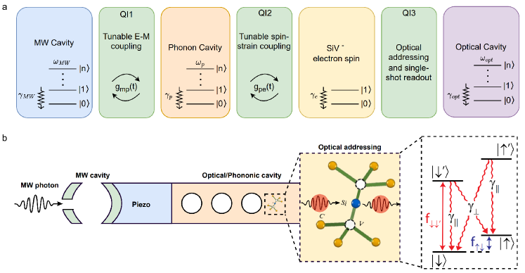
Fig.1 shows the overall schematic of the various quantum interfaces involved in the detection protocol. The first step of the scheme is to cool down the phonon cavity and initialize the spin state using the spin-photon interface (QI3). During the laser initialization process, the external B-field is tuned such that the spin-qubit frequency of the electron spin in SiV- matches the resonance frequency of the phononic crystal. The laser is parked at the frequency and thus, due to the nonzero cyclicity of optical transitions in SiV, after a sufficient time the spin gets initialized to the state. During this process, since electron spin is also resonantly tuned with the phononic crystal, the SiV also acts as a heat sink for the phonons, thereby cooling the phonon modes. However, the number of thermal phonons and thermal photons in the cavities is already very low, as we assume that the system is in thermal equilibrium with a dilution refrigerator at mK temperatures, which corresponds to .
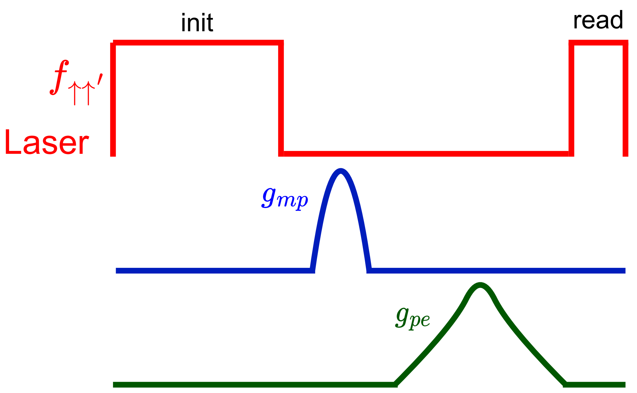
After the initialization, we detune the spin from phonon modes thereby effectively switching off , and switching on the tunable E-M coupling (QI1). This coupling is mediated via a piezoelectric transducer and acts as a gated detection window. The pulse is precharacterized such that it implements a swap operation between MW and phonon modes. Thus, if there is a MW photon in the cavity before the detection window, it gets swapped to a single phonon state in the phononic cavity. After the swap operation, we switch off the coupling and switch on the spin-strain coupling (QI2) again to perform the swap operation between the electron spin and the phonon mode. After this step, we switch off and perform single-shot readout of the electron spin using the spin-photon interface (QI3). The pulse-level schematic of the whole process can be seen in Fig. 2. In the presence of a MW photon in the cavity, one would then expect the electron spin to be in excited state with some fidelity, which will now depend on the swap fidelities and the readout fidelity. After this step, we reset the system by cooling the spin-phonon modes as done in the first step, and repeat the process.
2.1 Quantum-state transduction
The Hamiltonian describing the transduction involving the MW, phonon, and spin degrees of freedom is given by:
| (1) |
Here is the MW cavity annihilation (creation) operator, is the phononic cavity annihilation (creation) operator, and is the electron spin lowering (raising) operator. The frequencies , , and correspond to the MW, phonon, and electron-spin qubit, respectively. To incorporate losses into the system, we use the Lindblad equation of motion for the density matrix , and the Lindblad superoperators :
| (2) |
where
| (3) |
with , and which represents the decay (decoherence) rates of the respective modes. The Lindblad superoperators and describe the processes of MW cavity decay and phonon decay, respectively. The super-operator describes the process of pure dephasing of the electron spin qubit. The reason for not including the processes for the MW cavity and phonon mode is that we consider the rates of the processes corresponding to the times that are experimentally achievable. Since we assume the system to be operated at mK temperatures, we can neglect the thermal occupation of the modes.
As can be seen from Fig. 2, the state-transfer protocol is based on two swap operations mediated by pulses and . From a previous work[34] on quantum state transduction, in order to avoid high-frequency components, we assume that the couplings have a smooth dependence on time given by
| (4) |
| (5) |
where , are time-independent amplitudes and , are time delays for the respective pulses. The time delay between pulses = can be further adjusted for a given value of the parameters [] in order to optimize the state-transfer fidelity defined as:
| (6) |
where and is the density matrix corresponding to the initial state of the MW cavity, and final state of electron spin.
2.2 Protocol for cavity-enhanced single-shot readout
After the two swap operations and optimizing the pulse delays, we perform cavity enhanced single-shot readout of the SiV- electron spin. Optical readout of solid-state qubits is typically based on resonance fluorescence, and the readout fidelity is limited by the branching ratio corresponding to the spin-flipping transitions. For silicon vacancies, the branching ratio depends on the alignment angle of the static B-field with the SiV- symmetry axis. In the previous work[28], for a cyclicity of more than was achieved and despite the low photon collection efficiency, with a laser readout time of 10 ms a single shot readout fidelity of was demonstrated.
Since the laser readout time determines the detection time of our protocol, a low laser readout time is preferable. Since SiV- is a group-IV color center and is first order insensitive to electric field (unlike NV-centers), the readout time can be reduced by several orders of magnitude and the photon collection efficiency can be improved to above by integrating them in nanostructures[36].
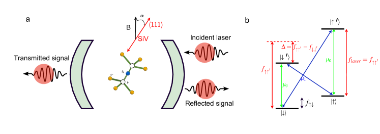
We consider the architecture as in Fig. 3a, where SiV- is in an optical cavity. Fig. 3b, shows the -type energy structure corresponding to two of the C-transitions of the SiV-. The parameters and represent the transition dipole moment of the dipole-allowed spin-conserving and dipole-forbidden spin-flipping optical transitions, respectively. We assume that we are in the SiV strain regime for which so that we can neglect the laser induced transitions. For performing optical readout, the optical cavity is in resonance with the transition and is detuned from the transition by . In this regime of operation, the atom-cavity coupling depends on the spin state, which also affects the reflection and transmission coefficients of the cavity. Hence, by probing the transmission/reflection coefficient we can perform a non-destructive single-shot readout of the spin state. Here, we proceed with probing the transmission coefficent as it is less sensitive to mode matching.
During the readout step, the cavity transmittivity is resonantly probed using a laser pulse of duration , with an incident photon flux of (units of number of photons per unit time). In the weak excitation regime (i.e. , where is the modified lifetime of the state), the average number of transmitted photons are given by[37, 38]
| (7) |
| (8) |
where and correspond to the average number of collected photons when the spin is in and state respectively, is the overall photon collection efficiency taking into account the coupling efficiency of the optics, imperfect spatial mode matching between the incident photon and the cavity, and quantum efficiency of the detector. The atomic cooperativity of the cavity is defined by = , where is the coupling strength between the cavity and transition, is the cavity decay rate, and is the decay rate of the excited state.
In order to determine the spin state, we pre-determine a threshold number , comparing the number of collected photons with . When , we report the spin state to be (presence of a MW photon), whereas when we report the spin state to be (absence of a MW photon). There are multiple metrics that can be obtained based on the above classification scheme as seen in Fig. 4.
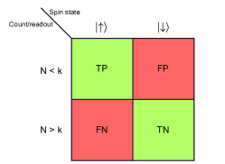
Assuming that the distribution of the collected photons is a Poissonian, we get the following expressions for the four metrics,
| (9) |
| (10) |
| (11) |
| (12) |
where we use the following nomenclature, TP: True Positive, TN: True Negative, FP: False Positive, FN: False Negative. Based on the above expressions, following figure of merits can be deduced, success probability , Shannon’s mutual information and dark count rate defined as,
| (13) |
| (14) |
| (15) |
where and is the probability that the spin is in the state and state respectively, X and Y are the distributions for the spin-state and their predictions respectively, is the time for the complete protocol. As can be seen from Fig. 5a, both and depend on the threshold parameter . Hence, for each set of parameters, an optimum value of can be obtained which maximizes or . From Fig. 5b, we can see that at optimal value of k, and are high whereas and are low, as demanded by the detection protocol. Depending on the rarity of the detection event and sensitivity required, different figure of merits can be used. For example for anomaly detection, it has been proposed[39] that Rényi information is more sensitive than Shannon information due to its asymmetric form. For this paper, we use and as the figure of merit of our protocol.
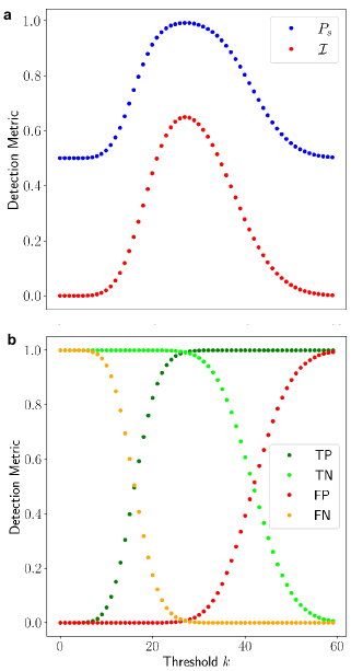
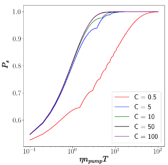
Fig. 6, shows the variation of w.r.t. laser readout time and cooperativity . We see that increases monotonically with as it leads to more collection time for the photons. For a given value of cooperativity, there exists a sufficiently long probe duration that leads to a near-unity success probability. However, this picture is incomplete as we didn’t include the spin-flip effect, which will increase with . Hence, we need to consider a model which incorporates this effect and cannot proceed with Eq. 7 and 8.
Eq. (9-15) remains valid even in the presence of spin-flip effects due to coupling to phonons or other spins. But the expression for and need to be evaluated from the following expression
| (16) |
where represents the annihilation operator for the cavity mode, is the density matrix of the spin-cavity system at time , for the initial states and respectively. We can numerically solve for by using the Lindblad master equation similar to Eq. (2), for the following readout Hamiltonian in the reference frame w.r.t to the laser frequency :
| (17) |
To incorporate losses, we use Eq. (3) of Lindblad superoperators with a new set of decay parameters, , and . Here and correspond to the spin-conserving decays, and correspond to the spin-flip decays, corresponds to the pure dephasing rate for the states and . The incident field amplitude of the laser given by is chosen to be much smaller than , so that we stay in the weak field linear regime.
3 Numerical simulation
In this section, we discuss the simulation of the detection protocol. The protocol can be divided into two parts, the first is the quantum state transduction and the second is the single-shot readout. The protocol has three metrics: detection time , the success probability , and the bandwidth. The detection bandwidth is determined by the piezoelectric transduction, and the detection time is governed by the transduction time and the readout time, whereas the success probability is determined by cavity parameters, readout time, external B-field, and its alignment with the SiV symmetry axis. Since there are various parameters involved, we use realistic values from previously demonstrated platforms, so that the evaluated detection metrics are experimentally realizable.
| Parameters | Values |
|---|---|
| 10 MHz[34] | |
| 1 MHz[34] | |
| 10 kHz[34] | |
| 100 Hz[34] | |
| 10 kHz[34] | |
| 5.5 GHz[35] |
| Parameters | Values |
|---|---|
| 8 GHz[36] | |
| 21 GHz[36] | |
| 0.1 GHz[35] | |
| 0.02 GHz[35] | |
| 0.25 MHz[28] | |
| 406.7 THz[35] | |
| 2.5 GHz[35] | |
| [37] | |
| 0.85[36] |
For the first part of quantum state transduction, we use the following values of the parameters for our simulation, MHz, MHz, kHz, Hz, kHz, GHz, which can be seen from table 1. Fig. 7 shows the simulation for quantum state transduction. We vary the time delay between the pulses, to optimize the state-transfer fidelity, and were able to achieve a fidelity of for ns. From Fig. 7e and 7f, we can see that the fidelity can be further increased upto 0.997 for of 1 kHz. The total duration of the first part of the protocol is 800 ns.
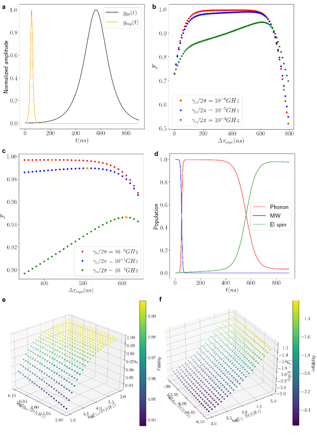
For the second part of single-shot readout, we use the following parameter values for simulation, GHz, GHz, 0.1 GHz, 0.02 GHz, MHz, THz, GHz, , 0.85, as seen in table 2. Many of these parameters depend on the experimental conditions and the SiV sample. For example, decay parameters depend on local strain environment of SiV- and the orientation of -field w.r.t. to SiV symmetry axis, the dephasing rate depends on and -field, depends on -field as well, the overall photon collection efficiency depends on fiber coupling, efficiency of other optical components, quantum efficiency of SNSPDs, etc. Hence, given a sample and experimental condition, different parameters can lead to a different optimal value. For our simulation, we use the above values to demonstrate the feasibility of this approach, but the same protocol can still be applied for different experimental conditions.
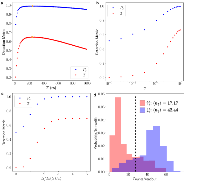
For the simulation of single-shot readout of electron spin, first we vary the laser readout time. For each readout time, we select the optimum value of , which individually maximizes and . For a large value of the metrics start to reduce due to the laser induced spin-flip effect. Hence, we select the probe time which maximizes and , as can be seen from Fig. 8a. For our simulation parameters, we obtain ns, for the = 0.9926 0.0003[36] and . As a next part of simulation, we use this value of and vary the photon collection efficiency, to estimate how much the chosen system can compromise on the collection efficiency without losing much on its detection probability. From Fig. 8b, we estimate that even for an efficiency of 22, would still be above 0.9. As approaches unity, tends to 0.996, whereas approaches to . For SiV, due to the anistropy in g-factor, the parameter is proportional to the static B-field. From Fig. 8c, we see that as is increased, tends to near unity and approaches to . A Shannon mutual information of implies that we get one bit of information about from , meaning a perfect, deterministic relationship between the random variables and . For = 5 GHz (corresponding to an achievable T and [35]), we estimate a of 0.9999 and of , meaning a perfect readout of the spin-states.
Next, we run a quantum Monte Carlo simulation for the single-shot read-out Hamiltonian given in Eq. (17), for 1000 trajectories and estimate the distribution of the number of clicks over the trajectories. Depending on whether the initial spin (MW) state is (1 MW photon) or (0 MW photon), the histogram plots change in shape, as seen in Fig. 8d with the dashed line representing the thresholding number in order to classify an event as MW detection or not.
To combine the two parts of the protocol and to estimate the overall detection metrics: , , , we multiply the two confusion matrices for the transduction and readout respectively and estimate a value of , , , with total time of the protocol 2 (800 + 214 + 1 ) after including an approximate laser initialization time of 1 . These metrics are function of the chosen parameters, experimental regime, and sample we choose to work with, and can be increased by improving the interface design in the transduction step, as the readout step is near-deterministic.
4 Conclusion
We proposed and simulated a method for gated detection of single MW photons in a cavity using a hybrid spin-optomechanical interface and obtained high detection efficiency of , dark count rate of , and Shannon mutual information of with experimentally realizable parameters. The efficiency is larger than that of the various alternatives[18, 19, 20, 21, 22, 23, 24, 31] for which the efficiency varies from 0.4-0.9. There exist platforms[21] which have a lower dark count rate of , but they suffer from low detection efficiency of . Hence, there is always a trade-off among the various detection metrics that can be obtained. There are various possible alternatives and extensions to the proposed scheme. For example first, to readout instead of working in the low cavity detuning regime, one can work in the high cavity detuning regime, and use the cavity resonance frequency as a metric for detection[35, 40] (instead of transmission coefficient). Second, instead of working in the single SiV regime, one could use an ensemble of SiVs in a phononic cavity and perform a dispersive readout using the phonon cavity. This method can also possibly be extended as a phonon detection and counter[40].
5 Acknowledgements
References
- [1] Kimble, H. J., Dagenais, M. & Mandel, L. Photon antibunching in resonance fluorescence. \JournalTitlePhys. Rev. Lett. 39, 691–695, DOI: 10.1103/PhysRevLett.39.691 (1977).
- [2] Hong, C. K. & Mandel, L. Experimental realization of a localized one-photon state. \JournalTitlePhys. Rev. Lett. 56, 58–60, DOI: 10.1103/PhysRevLett.56.58 (1986).
- [3] Beveratos, A. et al. Single photon quantum cryptography. \JournalTitlePhys. Rev. Lett. 89, 187901, DOI: 10.1103/PhysRevLett.89.187901 (2002).
- [4] Uppu, R. et al. Scalable integrated single-photon source. \JournalTitleScience Advances 6, DOI: 10.1126/sciadv.abc8268 (2020).
- [5] Zoller, P. et al. Quantum information processing and communication. \JournalTitleEur. Phys. J. D 36, 203–228 (2005).
- [6] Ekert, A. K. Quantum cryptography based on bell’s theorem. \JournalTitlePhys. Rev. Lett. 67, 661–663, DOI: 10.1103/PhysRevLett.67.661 (1991).
- [7] Cirac, J. I., Zoller, P., Kimble, H. J. & Mabuchi, H. Quantum state transfer and entanglement distribution among distant nodes in a quantum network. \JournalTitlePhys. Rev. Lett. 78, 3221–3224, DOI: 10.1103/PhysRevLett.78.3221 (1997).
- [8] Duan, L.-M., Lukin, M. D., Cirac, J. I. & Zoller, P. Long-distance quantum communication with atomic ensembles and linear optics. \JournalTitleNature 414, 413–418, DOI: 10.1038/35106500 (2001).
- [9] Spiller, T. P. et al. Quantum computation by communication. \JournalTitleNew Journal of Physics 8, 30–30, DOI: 10.1088/1367-2630/8/2/030 (2006).
- [10] Giovannetti, V., Lloyd, S. & Maccone, L. Quantum-enhanced measurements: Beating the standard quantum limit. \JournalTitleScience 306, 1330–1336, DOI: 10.1126/science.1104149 (2004).
- [11] Kimble, H. J. The quantum internet. \JournalTitleNature 453, 1023–1030, DOI: 10.1038/nature07127 (2008).
- [12] Nielsen, M. A. & Chuang, I. L. Quantum Computation and Quantum Information (Cambridge University Press, Cambridge, England, 2012).
- [13] Hadfield, R. H. Single-photon detectors for optical quantum information applications. \JournalTitleNat. Photonics 3, 696–705 (2009).
- [14] Eisaman, M. D., Fan, J., Migdall, A. & Polyakov, S. V. Invited review article: Single-photon sources and detectors. \JournalTitleRev. Sci. Instrum. 82, 071101 (2011).
- [15] Bergeal, N. et al. Analog information processing at the quantum limit with a josephson ring modulator (2009). 0805.3452.
- [16] Macklin, C. et al. A near-quantum-limited josephson traveling-wave parametric amplifier. \JournalTitleScience 350, 307–310 (2015).
- [17] Lang, C. et al. Correlations, indistinguishability and entanglement in Hong–Ou–Mandel experiments at microwave frequencies. \JournalTitleNat. Phys. 9, 345–348 (2013).
- [18] Gu, X., Kockum, A. F., Miranowicz, A., Liu, Y.-X. & Nori, F. Microwave photonics with superconducting quantum circuits. \JournalTitlePhys. Rep. 718-719, 1–102 (2017).
- [19] Romero, G., García-Ripoll, J. J. & Solano, E. Microwave photon detector in circuit qed. \JournalTitlePhys. Rev. Lett. 102, 173602, DOI: 10.1103/PhysRevLett.102.173602 (2009).
- [20] Peropadre, B. et al. Approaching perfect microwave photodetection in circuit qed. \JournalTitlePhys. Rev. A 84, 063834, DOI: 10.1103/PhysRevA.84.063834 (2011).
- [21] Balembois, L. et al. Practical single microwave photon counter with sensitivity (2023). 2307.03614.
- [22] Chen, Y.-F. et al. Microwave photon counter based on josephson junctions. \JournalTitlePhys. Rev. Lett. 107, 217401, DOI: 10.1103/PhysRevLett.107.217401 (2011).
- [23] Sathyamoorthy, S. R., Stace, T. M. & Johansson, G. Detecting itinerant single microwave photons. \JournalTitleC. R. Phys. 17, 756–765 (2016).
- [24] Inomata, K. et al. Single microwave-photon detector using an artificial -type three-level system. \JournalTitleNat. Commun. 7, 12303 (2016).
- [25] Barzanjeh, S., de Oliveira, M. C. & Pirandola, S. Microwave photodetection with electro-opto-mechanical systems (2014). 1410.4024.
- [26] Cornia, S. et al. Calibration‐free and high‐sensitivity microwave detectors based on InAs/InP nanowire double quantum dots. \JournalTitleAdv. Funct. Mater. 33 (2023).
- [27] Wong, C. H. & Vavilov, M. G. Quantum efficiency of a single microwave photon detector based on a semiconductor double quantum dot. \JournalTitlePhys. Rev. A (Coll. Park.) 95 (2017).
- [28] Sukachev, D. D. et al. Silicon-vacancy spin qubit in diamond: A quantum memory exceeding 10 ms with single-shot state readout. \JournalTitlePhys. Rev. Lett. 119, 223602, DOI: 10.1103/PhysRevLett.119.223602 (2017).
- [29] Wu, M., Zeuthen, E., Balram, K. C. & Srinivasan, K. Microwave-to-optical transduction using a mechanical supermode for coupling piezoelectric and optomechanical resonators. \JournalTitlePhysical Review Applied 13, DOI: 10.1103/physrevapplied.13.014027 (2020).
- [30] Li, P.-B. et al. Hybrid quantum device based onNVCenters in diamond nanomechanical resonators plus superconducting waveguide cavities. \JournalTitlePhys. Rev. Appl. 4 (2015).
- [31] Woodman, O., Pasharavesh, A., Wilson, C. & Bajcsy, M. Detecting single microwave photons with NV centers in diamond. \JournalTitleMaterials (Basel) 16 (2023).
- [32] Maity, S. et al. Coherent acoustic control of a single silicon vacancy spin in diamond. \JournalTitleNat. Commun. 11, 193 (2020).
- [33] Meesala, S. et al. Strain engineering of the silicon-vacancy center in diamond. \JournalTitlePhys. Rev. B 97, 205444, DOI: 10.1103/PhysRevB.97.205444 (2018).
- [34] Neuman, T. et al. A phononic interface between a superconducting quantum processor and quantum networked spin memories. \JournalTitleNpj Quantum Inf. 7 (2021).
- [35] Nguyen, C. T. et al. An integrated nanophotonic quantum register based on silicon-vacancy spins in diamond. \JournalTitlePhys. Rev. B 100, 165428, DOI: 10.1103/PhysRevB.100.165428 (2019).
- [36] Bhaskar, M. K. et al. Experimental demonstration of memory-enhanced quantum communication. \JournalTitleNature 580, 60–64 (2020).
- [37] Sun, S. & Waks, E. Single-shot optical readout of a quantum bit using cavity quantum electrodynamics. \JournalTitlePhysical Review A 94, DOI: 10.1103/physreva.94.012307 (2016).
- [38] Sun, S., Kim, H., Solomon, G. S. & Waks, E. Cavity-enhanced optical readout of a single solid-state spin. \JournalTitlePhysical Review Applied 9, DOI: 10.1103/physrevapplied.9.054013 (2018).
- [39] Kopylova, Y., Buell, D. A., Huang, C.-T. & Janies, J. Mutual information applied to anomaly detection. \JournalTitleJournal of Communications and Networks 10, 89–97, DOI: 10.1109/JCN.2008.6388332 (2008).
- [40] Wang, R.-X., Cai, K., Yin, Z.-Q. & Long, G.-L. Quantum memory and non-demolition measurement of single phonon state with nitrogen-vacancy centers ensemble. \JournalTitleOptics Express 25, 30149, DOI: 10.1364/oe.25.030149 (2017).
- [41] Johansson, P. N. . J. QuTiP - Quantum Toolbox in Python — qutip.org. https://qutip.org/.
- [42] GitHub - panand2257/Single-Photon-Detection: Single MW photon detection — github.com. https://github.com/panand2257/Single-Photon-Detection (2024).