Cyclically operated Single Microwave Photon Counter with sensitivity.
Abstract
Single photon detection played an important role in the development of quantum optics. Its implementation in the microwave domain is challenging because the photon energy is 5 orders of magnitude smaller. In recent years, significant progress has been made in developing single microwave photon detectors (SMPDs) based on superconducting quantum bits or bolometers. In this paper we present a practical SMPD based on the irreversible transfer of an incoming photon to the excited state of a transmon qubit by a four-wave mixing process. This device achieves a detection efficiency and an operational dark count rate , mainly due to the out-of-equilibrium microwave photons in the input line. The corresponding power sensitivity is , one order of magnitude lower than the state of the art. The detector operates continuously over hour timescales with a duty cycle , and offers frequency tunability of at least 50 MHz around 7 GHz.
Single photon detection is a mature technique in the optical domain. Its applications are numerous, ranging from fluorescence microscopy Orrit and Bernard (1990); Klar et al. (2000); Betzig et al. (2006); Bruschini et al. (2019) to measurement-based quantum computing Hadfield . At microwave frequencies ( GHz), single-photon detection is more challenging due to the five orders of magnitude photon energy, requiring in particular millikelvin temperatures to minimize the number of thermal photons per mode. Nevertheless, a range of applications make the development of such devices relevant. Single Microwave Photon Detectors (SMPDs) have been proposed for detecting weak incoherent emitters at microwave frequencies, such as electron spins in solids Albertinale et al. (2021); Billaud et al. ; Wang et al. (2023) or hypothetical dark matter candidate particles Lamoreaux et al. (2013); Dixit et al. . SMPDs may also be useful for primary thermometry Scigliuzzo et al. (2020) and for quantum illumination protocols Assouly et al. (2023). Finally, SMPDs will enable the implementation of several quantum information processing protocols Raussendorf et al. ; Briegel et al. ; Bartolucci et al. , for instance for the heralded entanglement of superconducting qubits at a distance Narla et al. (2016), the development of new qubit readout schemes Opremcak et al. , or the robust generation of quantum states Besse et al. .
SMPD designs based either on superconducting quantum bits or bolometers have been proposed Romero et al. (2009); Helmer et al. (2009); Sathyamoorthy et al. (2014); Kyriienko and Sørensen (2016); Sathyamoorthy et al. (2016); Gu et al. (2017); Wong and Vavilov (2017); Royer et al. (2018); Grimsmo et al. (2020) and implemented Chen et al. (2011); Koshino et al. (2013); Narla et al. (2016); Inomata et al. (2016); Besse et al. (2018); Kono et al. (2018); Lee et al. . Besides itinerant microwave photon detectors, other experiments have demonstrated high sensitivity detection of individual microwave photons in a high-Q cavity Schuster et al. (2007); Gleyzes et al. (2007); Dixit et al. .
The detection sensitivity, as well as the fidelity of the envisioned quantum protocols, depend crucially on the SMPD characteristics. Two figures of merit especially matter: the dark count rate defined as the number of false positive detection per unit of time, and the operational efficiency defined as the ratio of counts over incoming photons. Combining these two metrics, one can determine the power sensitivity of the detector as the noise equivalent power (NEP) for an integration time of 1 s (see Appendix C):
| (1) |
Currently, the detectors based on superconducting qubit Inomata et al. (2016); Besse et al. (2018); Kono et al. (2018) show a dark count rate , for an efficiency over a bandwidth of MHz, resulting in a sensitivity at 7 GHz. On the other hand, the most advanced bolometric detector based on graphene Lee et al. reaches a sensitivity at 7.9 GHz, when operated at 190 mK. The bandwidth of this device varies between 861 MHz and 599 MHz depending on the operating parameters.
This article presents a SMPD based on a superconducting qubit and a four-wave mixing process Lescanne et al. (2020). It detects itinerant photons, regardless of their waveform, in a 1 MHz bandwidth around a frequency tunable from 7.005 GHz to, at least, 6.955 GHz (see Appendix B) and operates by cycles of duration, which can be repeated continuously over several hours, days, or even months. Here we demonstrate, at the specific frequency of 6.979 GHz, a dark count rate for an operational efficiency leading to a power sensitivity , more than an order of magnitude lower than the state of the art. This new sensitivity has opened up new detection possibilities. In particular, a device (called SMPD2 in the following, Appendix I) very similar to the one discussed in this work has recently enabled the detection of individual electron spins in solids, through their microwave fluorescence Wang et al. (2023).
I Working principle
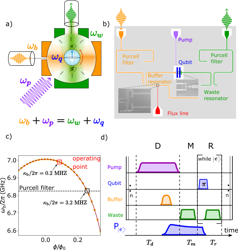
This device builds upon the superconducting circuit proposed and demonstrated in Lescanne et al. (2020) and Albertinale et al. (2021). The working principle is based on the irreversible transfer of an incoming photon to an excitation of a transmon qubit. The detector "clicks" when the qubit is detected in its excited state using dispersive readout through a capacitively coupled resonator.
This irreversible transfer is achieved by a four-wave mixing process, directly provided by the transmon qubit Hamiltonian. The incoming photon impinging on an input resonator with frequency (called "buffer" mode, orange in Fig. 1a) combines with a pump tone at frequency and is converted into an excitation in the transmon qubit mode at frequency and an additional photon in an output resonator mode at frequency (called "waste" mode, green in Fig. 1a). This four-wave mixing process is described by the Hamiltonian
| (2) |
where are the annihilation operators corresponding to the buffer mode and waste mode, is the lowering operator corresponding to the qubit, is the pump amplitude in the qubit mode, and , are the dispersive shifts of the transmon qubit with respect to the buffer and waste modes Lescanne et al. (2020). For this process to be activated, the pump frequency is tuned such that , to satisfy the four-wave mixing resonance condition.
The irreversibility of the conversion is ensured by the coupling of the waste resonator to a dissipative environment. While the qubit remains excited, the photon in the waste resonator leaks out in the measurement line at the rate . The reciprocal four-wave mixing process (second term in the parenthesis of Eq.(2)) is therefore suppressed and the qubit is left in its excited state. The detector behaves as an energy integrator, which is independent of the incoming photon waveform provided that its spectral extension remains included than the frequency linewidth of the buffer mode.
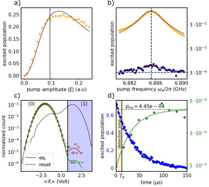
The four-wave mixing being a resonant process, it is intrinsically narrowband. To make it a practical detector, our device is made frequency tunable to match the photon frequency of interest by inserting a SQUID in the buffer resonator (see Fig. 1b). The detector frequency can be tuned from GHz over several hundred of MHz (see Fig. 1c). Two band-pass Purcell filters are associated with the resonators to prevent spurious decay of the qubit into the lines Sete et al. (2015). Therefore, the buffer resonator linewidth depends on its frequency detuning with respect to its Purcell filter. The bandwidth MHz is maximal for GHz. In the following, the detector is characterized at GHz and MHz. The resonance frequencies of the waste resonator GHz and the transmon qubit GHz are fixed. The relaxation time of the transmon qubit is measured to (see Fig. 2d) and its equilibrium population fluctuates around (see Fig. 2c,d), close to the lowest reported Serniak et al. (2018, 2019); Jin et al. (2015); Connolly et al. (2023). For the particular value GHz, the pump tone set by the four-wave mixing resonance condition becomes resonant with the buffer resonator. Under such conditions, the pump couples directly to the buffer, the four-wave mixing becomes degenerate, and the SMPD cannot operate. This collision between the pump and buffer frequencies is due to fabrication inaccuracies and has been corrected in the second version of the design (SMPD2 Appendix I).
The optimal pump characteristics (frequency and amplitude ) are determined experimentally by monitoring the qubit population while illuminating the buffer mode with a weak coherent signal and by sweeping the pump tone frequency and amplitude. As shown in Fig. 2b, a large excited state population is found in the qubit state conditioned on the presence of the illuminating tone for a pump frequency of GHz. This value is in good agreement with the mode frequencies taking into account the qubit Stark shift induced by the pump and the dispersive shift of the resonators.
In a restricted subspace where the buffer and the waste are never simultaneously populated, our device can be described by two cavities coupled with the strength Albertinale et al. (2021) (see Appendix D). In this framework, the maximum detection efficiency is expected when the coupling strength matches the geometric mean of decay rates of the buffer and waste resonators such that Lescanne et al. (2020). The model also provides an explicit formula for the transfer efficiency between a buffer photon and a qubit excitation:
| (3) |
where is the cooperativity associated with the four-wave mixing. Unit transfer efficiency is reached for . Taking into account resonator losses, we expect a maximum transfer efficiency of (see Appendix E). To determine the pump amplitude corresponding to the optimal cooperativity, we operate the four-wave mixing for various pump amplitude by sending photons on the buffer resonator. The resulting qubit excited population, plotted in Fig. 2a, is in good agreement with the theoretical two-coupled cavities model. We have chosen to operate slightly below the optimum pump amplitude to mitigate the heating effects.
In order to avoid spurious qubit heating due to the pump tone, a low pump amplitude is desirable. This is conveniently achieved if the dispersive shifts are larger than the . Here, the measured dispersive shifts are , and the resonators linewidths (at the point considered) and . At unit cooperativity, the pump energy in unit of qubit excitation is . Note that the large dispersive shift between the resonators and the qubit are not detrimental for two reasons. First, the maximum number of excitation in modes during the transfer process never exceeds one, so that higher order non-linear terms do not contribute significantly to the dynamics as shown on Fig. 2b. Second, Purcell filters at the output of each of the resonators inhibit the spurious decay of the qubit into transmission lines.
II Cyclic operation
The detector is operated cyclically, with the operation cycle consisting of three subsequent steps (see Fig. 1d). The first one called "detection" (D) consists in applying to the qubit a pump pulse at frequency during a detection time (see Appendix G for calibration). If a photon enters into the buffer resonator, the four-wave mixing process triggers a qubit excitation and a dissipation of a photon into the waste resonator.
In the second step of the cycle called "measurement" (M), the qubit state is dispersively readout using the waste resonator during a measurement time . Note that the threshold used to discriminate the qubit ground and excited states is chosen to maximize the SMPD power sensitivity defined in Eq.(1). As shown in Figure 2c, this threshold favors the readout fidelity of the ground state at the expense of the readout fidelity of the excited state . The dark count is minimized at the expense of a moderate reduction of the efficiency.
The third step of the cycle consists of a conditional reset (R). If the qubit is previously found in its ground state, we directly go to the next cycle. If the qubit was found in its excited state, a -pulse is applied though the pump line and the qubit state is measured again, the procedure being repeated until the ground preparation succeeds. Owing to the high fidelity of the qubit ground state readout, we reset the qubit well below its equilibrium population as shown in Figure 2d, the reset infidelity is as low as . The reset step is non-deterministic, with an average reset time . For the reset to work optimally, the Quantum Non Demolition character of the measurement must be ensured. To meet this condition, we use a Traveling Wave Parametric Amplifier (TWPA) and we tune carefully the readout pulse length and amplitude. Moreover, the readout pulse frequency is detuned with the respect to the waste resonator frequency by the dispersive shift of the qubit, such that the readout pulse enters the resonator if and only if the qubit is in its excited state. This allows to enhance the Quantum Non Demolition character of the measurement when the qubit is in its ground state.
A waiting time of 1 is added at the end of the reset step to let the waste resonator return to its ground state. The average cycle time is , which sets the duty cycle of the detector . This quantity could be made arbitrary close to one by increasing the duration of the detection window. However, the qubit relaxation in a characteristic time (see Fig. 2d) sets an upper bound, by introducing a contribution to the overall efficiency, which actually limits the detection step duration.
The detector is operated by continuously repeating the cycle times per second. Its temporal resolution is determined by the detection time , whereas its dead-time is .
III Detection efficiency
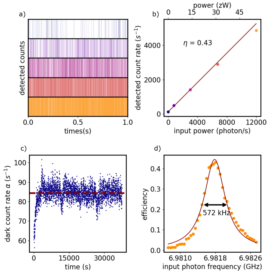
The operational efficiency is measured by sending a calibrated tone at the center of the SMPD line (see Fig. 3d) while the cycle is repeated. The power of the microwave tone is calibrated by using the dephasing of the qubit induced by the presence of photons in the buffer cavity Gambetta et al. (2006).
Typical measurement records of the detector for various illumination powers are shown Fig. 3a. The operational efficiency of the SMPD is obtained by measuring the ratio between the click event rate over the incoming photons rate as shown in Fig. 3b. The efficiency is in good agreement with the expected one that includes four different contributions: the transfer efficiency , the qubit relaxation , the duty cycle and the readout fidelity resulting into a theoretical efficiency .
IV Detection bandwidth
The detector bandwidth is measured by varying the frequency of a 10 photon pulse sent to the buffer resonator during the detection window. The qubit excitation probability is measured and multiplied by a constant factor so that the maximum value corresponds to the overall efficiency . This infered efficiency is then plotted with the respect to the frequency of the input photons as shown in Fig. 3d. The detector bandwidth, defined as the full width half-maximum is .
From a model of two coupled cavities (see Appendix D), explicitly derived in Albertinale et al. (2021), we can obtain an analytical expression of with respect to and :
| (4) |
yielding to the theoretical MHz. Here which corresponds to the limit where . We attribute the discrepancy between the theoretical and the measured bandwidth to the 100 kHz spectral broadening caused by the finite length of the excitation pulses.
V dark counts
The dark count rate is estimated by measuring the count-rate of the detector in the absence of input photons as illustrated on the top panel of Fig. 3a. The dark count rate is found to be 60 for few minute of the operation. As shown in Fig. 3c , when operated on hour time-scale, we observe a slight rise of the dark count rate to 85 during 1 hours, after what it remains stable within over 10 hours. The initial dark count rise is attributed to the heating of the cold stage of the refrigerator due to the continuous power delivered by the qubit pump. The sensitivity of the detector in steady state regime is then simply given by Eq. 1 and yields to a value .
VI dark count budget
The dark counts can be decomposed in three main contributions: the thermal population of the qubit , the heating of qubit by the pump , and the presence of thermal photons in the input lines . The resulting dark count rate is the sum of the three contributions: , each of them can be addressed individually.
The first contribution is the probability to find the qubit in its excited state in the absence of the four-wave mixing process. This depends on the qubit excitation probability after the reset and the relaxation rate of the qubit toward its equilibrium population (see Fig. 2c,d) such as . We evaluate this contribution to by using the parameters and defined in the previous sections. To mitigate this source of noise, the qubit is thermalized by filtering the line on a broad frequency range until the IR domain (eccosorb filter) and by properly designing an electromagnetic shield composed of 3 interleaved screens in metal, copper and aluminium (see appendix).
The second contribution is the spurious heating of the qubit by the pump tone . This contribution is measured by applying a pump tone detuned from the four-wave mixing condition while measuring the equilibrium population of the qubit. As shown in Fig.2b, in these conditions , a value included in the fluctuation interval of the equilibrium population. This contribution to the overall dark count rate is therefore considered negligible.
The third contribution is due to the presence of spurious photons in the input transmission lines. The integration of the mean number of photons per mode in the buffer input line over the linewidth of the detector gives the corresponding dark count rate . At the cryostat base temperature (10mK), this contribution should be negligible as the Planck law would predict an average number of photons per mode ; however, it is notoriously difficult to thermalize the microwave field at such low temperatures. Based on a Johnson-Nyquist description of thermal noise, we can derive the explicit relation Balembois (2023) (see Appendix F):
| (5) |
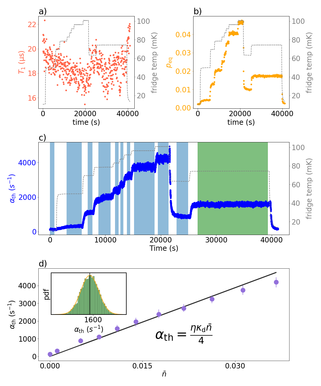
To verify the validity of this relation, we measure the thermal dark count as the function of a well defined mode population i.e when the refrigerator temperature is superior to 40 mK. This temperature is measured by a thermometer anchored to the mixing chamber plate. We acquired the dark count rate in a range from 10 mK to 100 mK, waiting for the end of the transient regime each time. Since the heating is not selective, all parts of the chip are affected including the transmon qubit which causes an increase in its equilibrium population and a decrease in its relaxation time . To take these effects into account, these two quantities are measured every minutes during the experiment (Fig. 4a,b), giving minute-by-minute monitoring of . Note that the relaxation time is now of the order of 20 compared with 37 in the previous sections. This decrease appeared for an unknown reason after a few cool-down cycles.
The thermal dark count rate is plotted as a function of time (see Fig. 4c) and with the respect to the thermal photon population calculated from the refrigerator temperature (see Fig. 4d). The relationship between and is linear with a slope of , therefore validating Eq. (5).
As explained earlier, at 10 mK, is decoupled from the refrigerator temperature, but we can estimate an equivalent electromagnetic temperature from the dark count measurement. At 10 mK, the measured dark count is (see Fig. 3c), as we evaluate to 5 , the equivalent is , corresponding to . By using Eq. (5), the equivalent electromagnetic temperature of the input line is 35 mK.
In principe, one could further improve the SMPD performances by improving the attenuation of the lines. However, the temperature of the microwave radiations is challenging to reduce arbitrarily close to the cryostat base temperature as it requires a large amount of attenuator that are well thermally anchored.
VII Conclusion
In conclusion, we have demonstrated the operation of a single microwave photon detector based on a four-wave mixing process.
The efficiency of the device reaches 0.43 and is quantitatively understood from the contributions of the detector duty cycle, the qubit ability to store an excitation, the qubit readout, and the 4 waves mixing efficiency. It can be improved in future devices with longer transmon relaxation times (see Appendix H), noting that qubit s up to several hundred microseconds have been demonstrated Place et al. ; Wang et al.
The second key quantity studied in this article is the dark count rate. We have demonstrated that most of these false positives events are caused by spurious photons due to the electromagnetic temperature of the line. A direct way of lowering the dark count would be to reduce the detector bandwidth so that it matches the bandwidth of the measured system.
Utilizing these metrics, the power sensitivity of the SMPD is determined as . We have also verified the direct relation between the count rates and the thermal occupation of the lines, opening the way to using the SMPD as an absolute thermometer in the 10-100mK range.
Even though further improvements of the device performance are desirable in the future, its high sensitivity already enabled new experiments, such as single-spin Electron Spin Resonance (ESR) spectroscopy Wang et al. (2023), as well as proof-of-principle axion search.
Acknowledgements
We acknowledge technical support from P. Sénat, D. Duet, P.-F. Orfila and S. Delprat, and are grateful for fruitful discussions within the Quantronics group. We acknowledge support from the Agence Nationale de la Recherche (ANR) through the DARKWADOR (ANR-19-CE47-0004) projects. We acknowledge support of the Région Ile-de-France through the DIM SIRTEQ (REIMIC project), from the AIDAS virtual joint laboratory, and from the France 2030 plan under the ANR-22-PETQ-0003 grant. This project has received funding from the European Research Council under grant no. 101042315 (INGENIOUS). We acknowledge IARPA and Lincoln Labs for providing the Josephson Traveling-Wave Parametric Amplifier.
Appendices
Appendix A Experimental parameters of the device
| Qubit | |||
| GHz | |||
| MHz | |||
| MHz | |||
| MHz | |||
| s | |||
| s | |||
| Buffer | top of arch | unbiased | at resonance |
| GHz | GHz | GHz | |
| MHz | MHz | MHz | |
| MHz | MHz | nc | |
| Waste | |||
| GHz | |||
| MHz | |||
| MHz | |||
| Filters | |||
| GHz | |||
| MHz | |||
| GHz | |||
| MHz |
The table summarises the various parameters of the device. The parameter () is the frequency of the waste (buffer) Purcell filter. are the filters bandwidth. is the anharmonicity of the qubit. is the coupling (internal) losses of the buffer resonator and is the coupling (internal) losses of the waste resonator.
Appendix B Other operating points
In the main text, we present the SMPD for the specific buffer frequency GHz. In this section, we present the dark count and the efficiency of the detector at two other buffer frequencies: GHz and GHz.
The efficiency is measured by sending a coherent wave packet of amplitude to the buffer for a time , while the four-wave mixing is activated by the pump tone (see Fig. 5a). The photon flux corresponding to the amplitude is calibrated using a Ramsey experiment perturbed by a field sent to the buffer (see Balembois (2023) for more details). For each time we measure the ratio between the number of photons sent and the qubit excited population, which gives the detector efficiency without the duty cycle contribution: . As shown in Fig. 5c, due to the buffer bandwidth, the efficiency grows with until it reaches an asymptote corresponding to . Taking into account the duty cycle, , we get for GHz and for GHz.
The dark count rate is measured by repeating the detection cycle times, where N is the number of experiments, and is the number of detection cycles of per experiment. For each experiment, the number of clicks per second is averaged over cycles and plotted as a function of time in Fig. 5d. We get for GHz and for GHz.
These figures give a sensitivity of for both buffer frequencies, comparable to the sensitivity shown in the main text.

Appendix C Noise Equivalent Power (NEP)
The NEP is defined as the minimum detectable power with an signal-to-noise ratio (SNR) of 1 for a certain integration time . This quantity, expressed in , provides a good representation of the absolute sensitivity of the SMDP.
We will first write the signal-to-noise ratio considering that the detected signal is provided by a continuous tone of power , at resonance with the buffer resonator and with a Poissonian noise. When this microwave tone is turning ON, the number of photon impinges the detector for a time is . Due to the dark count rate and the efficiency, the number of clicks given by the detector is . On the contrary, when the microwave tone is OFF, the signal integrated by the detector for a time is .
The signal of interest is . As all the distributions are Poissonian, the associated noise is . Assuming that the dark count is perfectly known we can reduce the expression of the noise to .
The SNR of the detection is then given by:
| (6) |
The NEP is given by the power corresponding to yielding to:
| (7) |
In this paper, the integration time is set such as reducing the NEP to:
| (8) |
Appendix D Two coupled cavities model
The detector response can be modeled by considering that the buffer and waste resonator are coupled with a constant due to the 4-wave parametric process involving the qubit, where is the pump amplitude in units of square root of photons and the dispersive coupling of the buffer (waste) resonator to the qubit. We can write down the system of coupled equations for the buffer and waste intra-resonator fields and , assuming that the resonators are lossless:
| (9) |
| (10) |
where and are the buffer and waste frequencies in the frame rotating at the probing frequency and , are the respective input field amplitudes. Now using the relation between the intra-resonator fields and the input and output flux , from the equilibrium solution of the coupled system we can extract the transmission coefficient . Assuming zero input flux on the waste this leads to:
| (11) |
or with the respect to the cooperativity :
| (12) |
This expression can be directly related to the detector efficiency as the input photon frequency is varied. The full-width-half-maximum of :
| (13) |
gives the bandwidth of the detector.
Appendix E Transmission coefficient in presence of buffer resonator losses
The effect of the buffer resonator internal losses on the efficiency can be evaluated by inserting (internal and coupling losses) in Eq (9). Assuming that the incoming photon and the pump frequencies are optimally tuned (i.e. ), the transmission coefficient becomes:
| (14) |
The maximization of with the respect of the cooperativity yields to:
| (15) |
The internal losses of the buffer resonator MHz combined with the external (coupling) losses MHz gives the maximum efficiency of the main text .
Appendix F Johnson-Nyquist noise
The thermal noise detected in the main text is described by a Johnson-Nyquist noise. In the classical framework, the noise power is expressed as a function of the detector bandwidth and the temperature of the experiment as: . In the quantum regime relevant for our experiment performed at low temperature 10 mK (), the average energy provided by the modes is given by Bose-Einsten statistics such as: with the number of photons per mode. The expression describing the flux of thermal photons per second is then:
| (16) |
To extract the extra number of clicks induced by this photon flux, we must take into account its conversion efficiency, which depends on the total detector efficiency , but also on its frequency detuning with the buffer resonator. In the limit where , we can consider that the conversion efficiency is given by a Lorentzian function centered around with a FWHM . This assumption yields the total number of extra clicks during a detection window:
| (17) |
| (18) |
Appendix G Otimization of the detection time
In the main text, we define the qubit efficiency as . This expression can approach 1 closely, by shortening the detection window, thereby diminishing the ratio . Nevertheless, reducing also decreases the duty cycle . One has thus to find a trade-off between and by maximizing the product:
| (19) |
In the limit where , the product takes the simple form:
| (20) |
The optimal detection window is then equal to :
| (21) |
Taking into account the parameters of our system, we choose .
Appendix H Effect of qubit relaxation time improvement on the SMPD sensitivity
Within the main text, we assert that augmenting the qubit’s stands as a pivotal factor in advancing the detector’s sensitivity to a greater extent. Indeed, an extended inherently enhances the efficiency of the qubit, . Furthermore, under the assumption of a constant , from eq. (21), it becomes apparent that the optimal detection time rises, thereby amplifying the duty cycle . An extended relaxation time contributes also to heightened readout efficiency, . It becomes possible to increase the readout time, , without encountering adverse effects from relaxation events during measurement. This naturally enhances the distinction between the two states within the phase plane.
The qubit relaxation time also plays a role in the SMPD dark count rate, as it appears directly in and indirectly in by the total efficiency .
Assuming that the of the device presented in the main text is larger by an order of magnitude, it follows that and . Concerning the dark count rate, and .
Under these conditions, we can estimate the new sensitivity would be (to be compared with the actual sensitivity ).
To further improve the sensitivity of the detector, it’s crucial to reduce the dark count rate due to the thermal population of the line. As mentioned in the main text, one option is to reduce the bandwidth of the detector to match the bandwidth of the system being measured. A detailed study of the dark count rate behaviour with the respect to the bandwith of the SMPD is given in Balembois (2023).
Appendix I Twin SMPD device
In the main text we present the characterisation of the first working device (SMPD1) with a sensitivity . A twin device (SMPD2) was fabricated a few months later to be used in a spin detection experiment Wang et al. (2023). Its resonator frequencies ( unbiased, ) and qubit frequency ( ) were chosen to optimise the detector performances around 7.3 . The qubit has a smaller lifetime, , and a comparable equilibrium population, . The measured efficiency and the measured dark count rate give an absolute sensitivity at 7.3 GHz. The table below shows the efficiency and dark count budget of the SMPD2 and how it compares with the SMPD1.
| Device | ||||
|---|---|---|---|---|
| SMPD1 | 5 | / | 80 | |
| SMPD2 | 9 | 2 | 90 | |
| SMPD1 | 0.84 | 0.76 | 0.86 | 0.84 |
| SMPD2 | 0.79 | 0.90 | 0.69 | 0.73 |
The decrease in and is due to the shorter , while the increase in is due to a cleaner calibration of the parametric amplifier. The SMPD2 buffer resonator present higher internal losses which translate into a smaller .
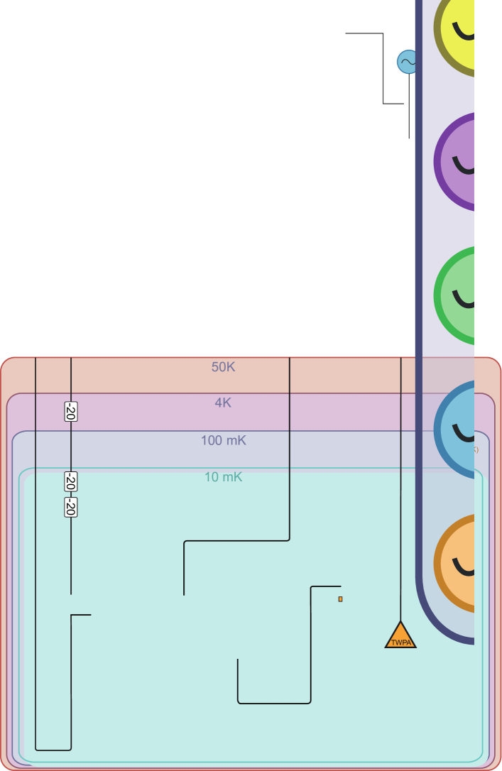
Appendix J Cryogenic setup
The figure 6 shows the wiring of the cryogenic setup used in this experiment. Lines 1 and 2 correspond to the detector input. They are used both to characterise the parameters of the buffer resonator () and to calibrate the detector efficiency by sending a well controlled number of photons. Line 3 is a DC flux bias line for tuning the SQUID inductance, which controls the frequency of the buffer resonator. Lines 4, 5 and 6 are used to probe the waste resonator to perform a dispersive readout of the qubit. Line 7 corresponds to the qubit drive.
References
- Orrit and Bernard (1990) M. Orrit and J. Bernard, Physical Review Letters 65, 2716 (1990).
- Klar et al. (2000) T. A. Klar, S. Jakobs, M. Dyba, A. Egner, and S. W. Hell, Proceedings of the National Academy of Sciences 97, 8206 (2000).
- Betzig et al. (2006) E. Betzig, G. H. Patterson, R. Sougrat, O. W. Lindwasser, S. Olenych, J. S. Bonifacino, M. W. Davidson, J. Lippincott-Schwartz, and H. F. Hess, Science 313, 1642 (2006).
- Bruschini et al. (2019) C. Bruschini, H. Homulle, I. M. Antolovic, S. Burri, and E. Charbon, Light: Science & Applications 8, 87 (2019).
- (5) R. H. Hadfield, 3, 696, number: 12 Publisher: Nature Publishing Group.
- Albertinale et al. (2021) E. Albertinale, L. Balembois, E. Billaud, V. Ranjan, D. Flanigan, T. Schenkel, D. Estève, D. Vion, P. Bertet, and E. Flurin, Nature 600, 434 (2021).
- (7) E. Billaud, L. Balembois, M. L. Dantec, M. Rančić, E. Albertinale, S. Bertaina, T. Chanelière, P. Goldner, D. Estève, D. Vion, P. Bertet, and E. Flurin, “Microwave fluorescence detection of spin echoes,” 2208.13586 [quant-ph] .
- Wang et al. (2023) Z. Wang, L. Balembois, M. Rančić, E. Billaud, M. L. Dantec, A. Ferrier, P. Goldner, S. Bertaina, T. Chanelière, D. Estève, D. Vion, P. Bertet, and E. Flurin, Nature 619, 276–281 (2023) (2023), https://doi.org/10.1038/s41586-023-06097-2.
- Lamoreaux et al. (2013) S. K. Lamoreaux, K. A. van Bibber, K. W. Lehnert, and G. Carosi, Physical Review D 88, 035020 (2013).
- (10) A. V. Dixit, S. Chakram, K. He, A. Agrawal, R. K. Naik, D. I. Schuster, and A. Chou, 126, 141302, 2008.12231 [hep-ex, physics:quant-ph] .
- Scigliuzzo et al. (2020) M. Scigliuzzo, A. Bengtsson, J.-C. Besse, A. Wallraff, P. Delsing, and S. Gasparinetti, Physical Review X 10, 041054 (2020), publisher: American Physical Society.
- Assouly et al. (2023) R. Assouly, R. Dassonneville, T. Peronnin, A. Bienfait, and B. Huard, Nature Physics 19, 1418 (2023), number: 10 Publisher: Nature Publishing Group.
- (13) R. Raussendorf, D. E. Browne, and H. J. Briegel, 68, 022312.
- (14) H. J. Briegel, D. E. Browne, W. Dür, R. Raussendorf, and M. Van den Nest, 5, 19, number: 1 Publisher: Nature Publishing Group.
- (15) S. Bartolucci, P. Birchall, H. Bombin, H. Cable, C. Dawson, M. Gimeno-Segovia, E. Johnston, K. Kieling, N. Nickerson, M. Pant, F. Pastawski, T. Rudolph, and C. Sparrow, “Fusion-based quantum computation,” 2101.09310 [quant-ph] .
- Narla et al. (2016) A. Narla, S. Shankar, M. Hatridge, Z. Leghtas, K. Sliwa, E. Zalys-Geller, S. Mundhada, W. Pfaff, L. Frunzio, R. Schoelkopf, and M. Devoret, Physical Review X 6, 031036 (2016).
- (17) A. Opremcak, I. V. Pechenezhskiy, C. Howington, B. G. Christensen, M. A. Beck, E. Leonard, J. Suttle, C. Wilen, K. N. Nesterov, G. J. Ribeill, T. Thorbeck, F. Schlenker, M. G. Vavilov, B. L. T. Plourde, and R. McDermott, 361, 1239, publisher: American Association for the Advancement of Science.
- (18) J.-C. Besse, S. Gasparinetti, M. C. Collodo, T. Walter, A. Remm, J. Krause, C. Eichler, and A. Wallraff, 10, 011046.
- Romero et al. (2009) G. Romero, J. J. García-Ripoll, and E. Solano, Physical Review Letters 102, 173602 (2009), publisher: American Physical Society.
- Helmer et al. (2009) F. Helmer, M. Mariantoni, E. Solano, and F. Marquardt, Physical Review A 79, 052115 (2009), publisher: American Physical Society.
- Sathyamoorthy et al. (2014) S. R. Sathyamoorthy, L. Tornberg, A. F. Kockum, B. Q. Baragiola, J. Combes, C. Wilson, T. M. Stace, and G. Johansson, Physical Review Letters 112, 093601 (2014), publisher: American Physical Society.
- Kyriienko and Sørensen (2016) O. Kyriienko and A. S. Sørensen, Physical Review Letters 117, 140503 (2016), publisher: American Physical Society.
- Sathyamoorthy et al. (2016) S. R. Sathyamoorthy, T. M. Stace, and G. Johansson, Comptes Rendus Physique Quantum microwaves / Micro-ondes quantiques, 17, 756 (2016).
- Gu et al. (2017) X. Gu, A. F. Kockum, A. Miranowicz, Y.-x. Liu, and F. Nori, Physics Reports Microwave photonics with superconducting quantum circuits, 718-719, 1 (2017).
- Wong and Vavilov (2017) C. H. Wong and M. G. Vavilov, Physical Review A 95, 012325 (2017), publisher: American Physical Society.
- Royer et al. (2018) B. Royer, A. L. Grimsmo, A. Choquette-Poitevin, and A. Blais, Physical Review Letters 120, 203602 (2018), arXiv: 1710.06040.
- Grimsmo et al. (2020) A. L. Grimsmo, B. Royer, J. M. Kreikebaum, Y. Ye, K. O’Brien, I. Siddiqi, and A. Blais, arXiv:2005.06483 [quant-ph] (2020), arXiv: 2005.06483.
- Chen et al. (2011) Y.-F. Chen, D. Hover, S. Sendelbach, L. Maurer, S. T. Merkel, E. J. Pritchett, F. K. Wilhelm, and R. McDermott, Physical Review Letters 107, 217401 (2011).
- Koshino et al. (2013) K. Koshino, K. Inomata, T. Yamamoto, and Y. Nakamura, Physical Review Letters 111, 153601 (2013), publisher: American Physical Society.
- Inomata et al. (2016) K. Inomata, Z. Lin, K. Koshino, W. D. Oliver, J.-S. Tsai, T. Yamamoto, and Y. Nakamura, Nature Communications 7, 12303 (2016).
- Besse et al. (2018) J.-C. Besse, S. Gasparinetti, M. C. Collodo, T. Walter, P. Kurpiers, M. Pechal, C. Eichler, and A. Wallraff, Physical Review X 8, 021003 (2018).
- Kono et al. (2018) S. Kono, K. Koshino, Y. Tabuchi, A. Noguchi, and Y. Nakamura, Nature Physics 14, 546 (2018).
- (33) G.-H. Lee, D. K. Efetov, W. Jung, L. Ranzani, E. D. Walsh, T. A. Ohki, T. Taniguchi, K. Watanabe, P. Kim, D. Englund, and K. C. Fong, 586, 42, number: 7827 Publisher: Nature Publishing Group.
- Schuster et al. (2007) D. I. Schuster, A. A. Houck, J. A. Schreier, A. Wallraff, J. M. Gambetta, A. Blais, L. Frunzio, J. Majer, B. Johnson, M. H. Devoret, S. M. Girvin, and R. J. Schoelkopf, Nature 445, 515 (2007).
- Gleyzes et al. (2007) S. Gleyzes, S. Kuhr, C. Guerlin, J. Bernu, S. Deléglise, U. Busk Hoff, M. Brune, J.-M. Raimond, and S. Haroche, Nature 446, 297 (2007).
- Lescanne et al. (2020) R. Lescanne, S. Deléglise, E. Albertinale, U. Réglade, T. Capelle, E. Ivanov, T. Jacqmin, Z. Leghtas, and E. Flurin, Physical Review X 10, 021038 (2020).
- Sete et al. (2015) E. A. Sete, J. M. Martinis, and A. N. Korotkov, Phys. Rev. A 92, 012325 (2015).
- Serniak et al. (2018) K. Serniak, M. Hays, G. de Lange, S. Diamond, S. Shankar, L. D. Burkhart, L. Frunzio, M. Houzet, and M. H. Devoret, Physical Review Letters 121, 157701 (2018), arXiv: 1803.00476.
- Serniak et al. (2019) K. Serniak, S. Diamond, M. Hays, V. Fatemi, S. Shankar, L. Frunzio, R. Schoelkopf, and M. Devoret, Phys. Rev. Appl. 12, 014052 (2019).
- Jin et al. (2015) X. Y. Jin, A. Kamal, A. P. Sears, T. Gudmundsen, D. Hover, J. Miloshi, R. Slattery, F. Yan, J. Yoder, T. P. Orlando, S. Gustavsson, and W. D. Oliver, Phys. Rev. Lett. 114, 240501 (2015).
- Connolly et al. (2023) T. Connolly, P. D. Kurilovich, S. Diamond, H. Nho, C. G. L. Bøttcher, L. I. Glazman, V. Fatemi, and M. H. Devoret, (2023), arXiv:2302.12330 [quant-ph] .
- Gambetta et al. (2006) J. Gambetta, A. Blais, D. I. Schuster, A. Wallraff, L. Frunzio, J. Majer, M. H. Devoret, S. M. Girvin, and R. J. Schoelkopf, Physical Review A 74, 042318 (2006).
- Balembois (2023) L. Balembois, Magnetic resonance of a single electron spin and its magnetic environment by photon counting, thesis, Paris Saclay (2023).
- (44) A. P. M. Place, L. V. H. Rodgers, P. Mundada, B. M. Smitham, M. Fitzpatrick, Z. Leng, A. Premkumar, J. Bryon, A. Vrajitoarea, S. Sussman, G. Cheng, T. Madhavan, H. K. Babla, X. H. Le, Y. Gang, B. Jäck, A. Gyenis, N. Yao, R. J. Cava, N. P. de Leon, and A. A. Houck, 12, 1779, number: 1 Publisher: Nature Publishing Group.
- (45) C. Wang, X. Li, H. Xu, Z. Li, J. Wang, Z. Yang, Z. Mi, X. Liang, T. Su, C. Yang, G. Wang, W. Wang, Y. Li, M. Chen, C. Li, K. Linghu, J. Han, Y. Zhang, Y. Feng, Y. Song, T. Ma, J. Zhang, R. Wang, P. Zhao, W. Liu, G. Xue, Y. Jin, and H. Yu, 8, 1, number: 1 Publisher: Nature Publishing Group.