New physics analysis of baryonic decays under SMEFT framework
Abstract
The di-leptons and di-neutrinos observed in the final states of flavor-changing neutral b decays provide an ideal platform for probing physics beyond the standard model. Although the latest measurements of agree well with the standard model prediction, there exists several other observables such as , and in transition decays that shows deviation from the standard model prediction. Similalry, very recently Belle II collaboration reported a more precise upper bound of by employing a new inclusive tagging approach and it also deviates from the standard model expectation. The and transition decays are related not only in the standard model but also in beyond the standard model physics due to gauge symmetry, and can be most effectively investigated using the standard model effective field theory formalism. Additionally, the decay channels are theoretically cleaner than the corresponding decays, as these processes do not get contributions from non-factorizable corrections and photonic penguin contributions. In this context, we study baryonic decays undergoing and quark level transitions in a standard model effective field theory formalism. We give predictions of several observables pertaining to these decay channels in the standard model and in case of several new physics scenarios.
I Introduction
In high-energy physics experiments, such as those at particle accelerators, it is possible to produce and detect intermediate states of quantum particles that have much greater mass than the initial and final particles. These intermediate states are often short-lived and can only be observed through the detection of their decay products. In this context, study of flavor changing charged current (FCCC) and neutral current (FCNC) transitions of hadrons is crucial as they can provide important information regarding such intermediate quantum states. Moreover, FCNC transition decays are, in principle, more sensitive to various new physics (NP) effects as they proceed either via loop level or box level diagrams where the intervention of heavier particles comes into the picture. Hence, study of these decays would offer a powerful tool to search for NP that lies beyond the standard model (SM). Over the past several years, the FCNC B decays have been the center of attention of the particle physics community especially due to discrepancies observed at BaBar, Belle and more recently at LHCb. The measured values of the lepton flavor sensitive observable such as the ratio of branching fractions and in decays deviate from the SM prediction. These discrepancies hint for a possible violation of lepton flavor universality (LFU) in transition decays.
Earlier LHCb measurement of in showed deviation from the SM expectation LHCb:2021trn . Similalry, earlier measurements of from both LHCb LHCb:2017avl ; LHCb:2020lmf and Belle Belle:2019oag in and bins showed deviation Bordone:2016gaq ; Hiller:2003js from SM. However, very recent LHCb results LHCb:2022qnv ; LHCb:2022zom , announced in December 2022, has completely changed the entire scenario. The latest measured values of and in and and in show an overall agreement with the SM prediction with standard deviation LHCb:2022qnv ; LHCb:2022zom .
Although and seem to be SM like, the possibilities of NP cannot be completely ruled out. Apart from and , there are several other observables where the discrepancy between the measured value and the SM prediction still exists. Measurement of from LHCb LHCb:2013ghj ; LHCb:2015svh and ATLAS ATLAS:2018gqc show deviation from the SM prediction. Similarly, CMS CMS and Belle Belle:2016xuo measurements show and deviations, respectively Descotes-Genon:2012isb ; Descotes-Genon:2013vna ; Descotes-Genon:2014uoa . Again, the measured value of the branching fraction of in deviates from the SM prediction at LHCb:2021zwz ; LHCb:2013tgx ; LHCb:2015wdu . Moreover, measurements of the ratio of branching ratio LHCb:2021lvy and , isospin partners of and , also deviate from the SM prediction at and , respectively.
There exists another class of FCNC transition decays with neutral leptons in the final state that are mediated via quark level transitions. Theoretically these di-neutrino channels are clean as they do not suffer from hadronic uncertainties beyond the form factors such as the non-factorizable corrections and photon penguin contributions. However, they are very challenging from the experimental point of view due to the presence of neutrinos in the final state. Inspite of that BaBar, Bell/Belle II has managed to provide the upper bounds of decays to be Dattola:2021cmw and , respectively. Combined with the previous measurements from Belle and BaBar one estimates the world average value of the branching fraction to be Dattola:2021cmw . A combined analysis of and decays is theoretically well motivated as these two channels are closely related not only in the SM but also in beyond the SM under gauge symmetry. Moreover, a more precise measurements of branching fraction in future may provide useful insight into NP that may be present in transition decays.
Various analyses, both model-dependent and model-independent, have been performed to account for these anomalies. A non-exhaustive compilation of relevant literature can be found in the references Rajeev:2021ntt ; Mohapatra:2021ynn ; Li:2011nf ; Huang:2018rys ; Falahati:2014yba ; Ahmed:2010tt ; Capdevila:2017bsm ; Bashiry:2009wq ; Wang:2012ab ; Li:2010ra ; Rajeev:2020aut ; Browder:2021hbl ; Bobeth:2001jm ; Altmannshofer:2009ma ; Descotes-Genon:2020buf ; Fajfer:2018bfj . To confirm the presence of NP, we need to perform measurements of similar observables in different decay processes that proceed via same quark level transitions. Similarly, it is very important to perform a detailed angular analysis in order to look for several form factor independent angular observables which are sensitive to NP. In this context, baryonic decay mode has got lot of attention. The recent measurement from LHCb suggests that although the ratio is compatible with SM, there is suppression in compared to LHCb:2019efc . To interprit this result, it is essential to have a precise theoretical knowledge of various excited states of baryon contributing to region. The decay to has the largest contribution among the various semileptonic modes of decays to hadrons. Due to its spin parity of and strong decay into the pair, the is readily distinguishable from nearby hadrons, including the , , and weakly decaying , which have a spin parity of . In Ref Meinel:2020owd ; Meinel:2021mdj , the authors calculate the LQCD form factors in the weak transition of decay, while in Ref. Descotes-Genon:2019dbw and Ref. Das:2020cpv , the authors performed angular analyses of decays for massless and massive leptons, respectively. Additionally, in Ref Amhis:2020phx , the authors investigated the angular distributions of and discussed the potential for identifying NP effects. Similalry, the authors in RefLi:2022nim study the process with and examine several angular observables. The study is performed with a set of operators where the SM operator basis is supplemented with its chirality flipped counterparts and new scalar and pseudoscalar operators. The three-body light-front quark model based on the gaussian expansion method is used to systematically investigate the () decay process. Several theoretical methods, such as lattice QCD (LQCD) Detmold:2012vy ; Detmold:2016pkz , QCD sum rules (QCDSR) Chen:2001sj , light-cone sum rule (LCSR) Aslam:2008hp ; Wang:2008sm ; Wang:2009hra ; Aliev:2010uy ; Wang:2015ndk , covariant quark model (CQM) Gutsche:2013pp , nonrelativistic quark model Mott:2011cx , and Bethe-Salpeter approach Liu:2019igt , have been used to study the rare decay . The initial measurement of the decay was conducted by the CDF Collaboration CDF:2011buy , followed by a subsequent measurement by the LHCb Collaboration LHCb:2015tgy ; LHCb:2018jna . In ref Huang:1998ek QCD sum rules were used to calculate the transition form factors and to study the unpolarized decay. The form factors for at large recoil were analyzed using a sum-rule approach to study spectator-scattering corrections Feldmann:2011xf . Light-cone distribution amplitude of wave function was studied in Ali:2012pn ; Bell:2013tfa ; Braun:2014npa to further understand the theoretical aspects. A model-independent analysis for unpolarized decay was performed in Das:2018sms ; Das:2018iap ; Das:2020cpv ; Roy:2017dum ; Yan:2019tgn using a complete set of dimension-six operators. The angular distribution of the decay with unpolarised baryon has been explored in Refs.Boer:2014kda ; Yan:2019tgn , while in Ref.Blake:2017une , the study involved polarized baryon. Furthermore, in Ref.Blake:2019guk , the Wilson coefficients were examined by utilizing the complete angular distribution of the rare decay measured by the LHCb Collaboration LHCb:2018jna . Similalry, in RefChen:2000mr , the authors calculate the branching fraction of decay by taking the polarised and . Moreover, in Ref Sirvanli:2007yq , the authors analyse decay by considering the model. Here the authors calculate the branching ratio as well as the longitudinal, transversal and normal polarizations of the di-neutrino decay channel of the baryonic decay within the SM as well as in the presence of leptophobic model.
In this paper, we study the implication of anomalies on and decays in a model independent way. Our work differs significantly from others. For NP analysis, we construct several and NP scenarios emerging out of dimension six operators in the standard model effective field theory (SMEFT) formalism. We obtain the allowed NP parameter space by performing a global fit to the data. Moreover, we also use the measured upper bound on to check the compatibility of our fit results.
The paper is organized as follows. In Section II, we start with a brief description of the SMEFT framework and write down the effective Hamiltonian for the and quark level transition decays. Subsequently, we report all the relevant formulae for the observables in Section II. In Section III, we first report all the input parameters that are used for our analysis. A detailed discussion of the results pertaining to and baryonic decay observables in the SM and in case of NP scenarios are also presented. Finally, we conclude with a brief summary of our results in Section IV.
II Theory
Till date, no direct evidence of new particles near the electroweak scale has been observed from searches conducted in the Large Hadron Collider (LHC). Nevertheless, these searches provide indirect evidence supporting the existence of NP at a scale beyond the electroweak scale. To explore indirect signatures of NP in a model-independent way, the SMEFT framework offers a more efficient approach. The SMEFT Lagrangian explains particle interactions in the SM and in all possibleextensions of SM. It is constructed by incorporating higher-dimensional operators into the SM Lagrangian while maintaining the gauge symmetry. These higher-dimensional operators are suppressed by a factor that depends on a new energy scale. The SMEFT Lagrangian comprises all sets of these higher-dimensional operators that are consistent with the underlying gauge symmetry. For investigating NP beyond the SM at low energies, this framework provides an excellent platform. From the fundamental aspect of the electroweak theory, the left-handed charged leptons are related to neutral leptons through the symmetry. In this study, we concentrate on the connection between and transition decays within the SMEFT framework by considering dimension six operators. If no new particles are observed at the LHC, it will imply a NP scale that is greater than the energy scale of the LHC. The SMEFT analysis would be crucial in this situation as it offers a way to examine the implications of NP indirectly by evaluating their effects on SM low energy processes.
The effective Lagrangian corresponding to dimension six operators is expressed as Grzadkowski:2010es
| (1) |
Among all the operators, the relevant operators contributing to both and decays are
| (2) |
Similarly, the operators contributing only to decays are
| (3) |
At low energy, the most general effective Hamiltonian governing both and decays can be written as Altmannshofer:2009ma ; Buras:2014fpa ,
| (4) |
where is the Fermi coupling constant, are the associated Cabibbo Kobayashi Maskawa (CKM) matrix elements. The sum comprises the operators with the corresponding WCs contributing to decays. They are
| (5) |
Here, represents the projection operator. In the SM, and the value of is calculated to be
| (6) |
Similarly, for , the sum comprises the operators with the corresponding WCs that contribute to decays. The operators are
| (7) |
In the presence of dimension six SMEFT operators, the WCs and get modified. They can be expressed as follows. Buras:2014fpa
| (8) |
where, , and represents the small vector coupling to charged leptons.
II.1 Differential decay distribution and dependent observables for decays
The four-fold angular distribution for decay can be expressed as Das:2020cpv
| (9) | |||||
where represents the angle formed by the proton with the daughter baryon in the rest frame of . Similarly, in the rest frame of the lepton pair, denotes the angle formed by the with respect to the direction of the daughter baryon . Moreover, in the rest frame of , defines the angle between the planes containing and the lepton pair. The angular coefficients , , can be expressed as
| (10) |
Here the first term corresponds to massless leptons, whereas, and correspond to linear () and quadratic () mass corrections, respectively. The explicit expressions for , and in terms of transversely amplitude are taken Ref Das:2020cpv .
From the Differential decay distributions, one can construct several physical observables.
-
•
The differential branching ratio , the lepton forward-backward asymmetry , the fraction of longitudinal polarization and the ratio of branching fraction are defined as
(11) -
•
We define several angular observables such as , , , , , , , , , , . They are
(12)
It is important to note that the angular coefficients (, ), (, ), and (, ) exhibit a strict relation in the SM. That is
| (13) |
II.2 Differential decay distribution and dependent observables for
The four fold angular distribution for is defined as Das:2018iap
| (14) | |||||
where the angular coefficients can be expressed as
| (15) |
with . The explicit expressions for , and are taken from Ref Das:2018iap .
We define several physical observables pertaining to this decay mode.
-
•
Differential branching ratio , the lepton forward-backward asymmetry , the fraction of longitudinal polarization and the ratio of branching fraction are defined as
(16) -
•
Angular observables such as , , , , , , , , , are defined as
(17)
III Results
III.1 Input parameters
The numerical values of all the input parameters used in the paper are summarized in the Table 1. Input parameters, such as the masses of mesons and quarks are expressed in GeV units, the Fermi coupling constant is in GeV-2 units and the life time of baryon is in seconds.
| Parameter | Value | Parameter | Value | Parameter | Value | Parameter | Value | Parameter | Value |
| 0.000511 | 0.105658 | 1.28 GeV | |||||||
| 5.619 GeV | 5.619 GeV | ||||||||
| 4.2 | 1.28 | 4.8 | |||||||
| 0.443 | 0.333 |
For hadronic inputs such as form factors, we use the values reported in Ref. Mott:2011cx , and for form factors, we use the LQCD results of Ref Detmold:2016pkz . The relevant formula for the form factors pertinent for our discussion is as follows Mott:2011cx
| (18) |
where
| (19) |
Here and . We consider uncertainty in the input parameters , and . The values of these parameter, taken from Ref Mott:2011cx , are reported in Table 2.
| form factor inputs | ||||||||||||||
| -1.66 | 0.544 | 0.126 | -0.0330 | -0.964 | 0.625 | -0.183 | 0.0530 | -1.08 | -0.507 | 0.187 | 0.0772 | -0.0517 | 0.0206 | |
| -0.295 | 0.194 | 0.00799 | -0.00977 | -0.100 | 0.219 | -0.0380 | 0.0161 | -0.0732 | -0.246 | 0.0295 | 0.0267 | -0.0173 | 0.00679 | |
| 0.00924 | -0.00420 | -0.000365 | 0.00211 | 0.00264 | -0.00508 | 0.00351 | -0.00221 | 0.00464 | 0.00309 | -0.00107 | -0.00217 | 0.00259 | -0.000220 | |
Similarly, for transition form factors, we use the relevant form factor formula from Ref Detmold:2016pkz . That is
| (20) |
To calculate the statistical uncertainties of the observable, we utilize the parameters from the ”nominal” fit. However, to estimate the systematic uncertainties, we use a ”higher-order” fit where the fit function is given by
| (21) |
The function is defined as
| (22) |
where and . The fit parameters and masses used in our analysis are taken from Ref. Detmold:2016pkz . For completeness, we report them in Table 3.
| Parameter | Value | Parameter | Value | |
| , , , | ||||
| , , , |
III.2 SM predictions
In this section, we present the central values and the uncertainties of several observables for the and decay channels. More specifically, we give prediction of the branching ratio (), the ratio of branching ratios (), the forward-backward asymmetry (), the longitudinal polarization fraction () for the modes, respectively. We also report various angular observables such as , , , , , , , for decay mode. Similarly, we report angular observables such as , , , , , , , , , for decay mode as well. Moreover, we give predictions of several observables pertaining to and decay modes. The central values of the observables are obtained using the central values of the input parameters, whereas the uncertainties in each observable are determined by varying the uncertainties associated with inputs such as form factors and the CKM matrix elements within of their central values. For the final states, we explore two bins, namely and for the decay mode and and for the decay mode, respectively. All the results are listed in Table 4 and Table. 5, respectively.
| decay | decay | ||||
| Observables | bin | Central value | range | Central value | range |
| BR | 1.1 - 6.0 | 6.063 | (4.660, 8.012) | 0.775 | (0.460, 1.164) |
| 14.2/15.0 - | 7.318 | (5.655, 9.100) | 3.723 | (3.105, 4.313 ) | |
| 1.1 - 6.0 | 0.781 | (0.760, 0.800) | 0.829 | (0.696, 0.907) | |
| 14.2/15.0 - | 0.430 | (0.424, 0.443) | 0.339 | (0.312, 0.375) | |
| 1.1 - 6.0 | -0.114 | (-0.135, -0.089) | -0.028 | (-0.146, 0.051) | |
| 14.2/15.0 - | -0.236 | (-0.274, -0.198) | -0.299 | (-0.330, -0.269) | |
| 1.1 - 6.0 | -0.152 | (-0.180, -0.119) | -0.019 | (-0.097, 0.034) | |
| 14.2/15.0 - | -0.313 | (-0.363, -0.262) | -0.199 | (-0.220, -0.180) | |
| 1.1 - 6.0 | 0.219 | (0.200, 0.239) | 0.086 | (0.046, 0.152) | |
| 14.2/15.0 - | 0.565 | (0.552, 0.573) | 0.331 | (0.313, 0.344) | |
| 1.1 - 6.0 | 0.890 | (0.880, 0.900) | 0.457 | (0.424, 0.477) | |
| 14.2/15.0 - | 0.713 | (0.719, 0.710) | 0.335 | (0.328, 0.344) | |
| 1.1 - 6.0 | -0.038 | (-0.045, -0.030) | 0.013 | (-0.012, 0.063) | |
| 14.2/15.0 - | -0.080 | (-0.093 ,-0.067) | 0.202 | (0.190, 0.210) | |
| 1.1 - 6.0 | 0.055 | (0.050, 0.060) | -0.054 | (-0.095, -0.029) | |
| 14.2/15.0 - | 0.145 | (0.142, 0.146) | -0.135 | (-0.149, -0.122) | |
| 1.1 - 6.0 | 0.223 | (0.220, 0.225) | -0.026 | (-0.048, -0.012) | |
| 14.2/15.0 - | 0.181 | (0.180, 0.182) | -0.067 | (-0.074, -0.061) | |
| 1.1 - 6.0 | 0.000 | (-0.001, 0.001) | |||
| 14.2/15.0 - | -0.032 | (-0.039, -0.027) | |||
| 1.1 - 6.0 | 0.003 | (-0.062, 0.078) | |||
| 14.2/15.0 - | -0.043 | (-0.057, -0.030) | |||
| 1.1 - 6.0 | 0.031 | (-0.057, 0.110) | |||
| 14.2/15.0 - | -0.116 | (-0.132, -0.100) | |||
| 1.1 - 6.0 | 0.014 | (0.011,0.018) | |||
| 14.2/15.0 - | 0.046 | (0.039, 0.055) | |||
| 1.1 - 6.0 | 0.996 | (0.996, 0.996) | 0.995 | (0.989, 1.007) | |
| 14.2/15.0 - | 0.993 | (0.993,0.993) | 1.007 | (1.006, 1.007) | |
| 1.1 - 6.0 | -0.000 | (-0.000, -0.000) | -0.011 | (-0.017, -0.007) | |
| 14.2/15.0 - | -0.000 | (0.000, 0.000) | 0.001 | (0.001,0.001) | |
| 1.1 - 6.0 | 0.000 | (0.000, 0.000) | 0.001 | (-0.000,0.003) | |
| 14.2/15.0 - | 0.001 | (0.001, 0.001) | -0.000 | (-0.000, -0.000) | |
| decay | decay | |||
| Observables | Central value | range | Central value | range |
| BR | 1.414 | (1.148, 1.743) | 1.795 | (1.406, 2.202) |
| 0.522 | (0.503, 0.547) | 0.472 | (0.395, 0.564) | |
| -0.421 | (-0.440, -0.391) | -0.207 | (-0.165, -0.241) | |
| 0.477 | (0.452, 0.497) | 0.264 | (0.218, 0.302) | |
| 0.760 | (0.751, 0.773) | 0.368 | (0.349, 0.391) | |
| -0.106 | (-0.110, -0.098) | 0.170 | (0.140, 0.194) | |
| 0.120 | (0.114, 0.125) | -0.133 | (-0.155, -0.106 ) | |
| 0.190 | (0.188, 0.193) | -0.066 | (-0.077, -0.053) | |
| -0.032 | (-0.060, 0.000) | |||
| -0.061 | (-0.099, -0.025) | |||
| -0.008 | (-0.011, -0.006) | |||
| 0.022 | (0.019, 0.026) | |||
Our observations are as follows.
-
•
The branching ratio of mode is found to be of , while the branching ratio of decay mode is observed to be of .
-
•
The values of , , , , , and are observed to be lower at high bin compared to the values obtained in the low bin.
-
•
In the case of the decay mode, values of and are zero in the low bin, whereas they are non-zero in the high bin.
-
•
We found the ratios , and to be equal to .
-
•
As expected, value of is very close to unity.
-
•
The branching fraction of both and decay channels are found to be of .
-
•
It is observed that the uncertainties in the di-neutrino channels are less than the uncertainty in di-lepton decay channels.
For completeness we also report the branching ratio for the mode to be in which is quite similar to the value reported in ref .Das:2018iap . A slight difference is observed due to the different choice of input parameters.
III.3 Global fit
Our primary objective in this work is to use a model-independent SMEFT formalism to investigate the effects of anomalies on several baryonic and transition decays. The SMEFT coefficients for left chiral currents, namely , , and contribute to WCs in and to in transitions decays. Similarly, the SMEFT coefficients for right chiral currents such as and are connected to in and in transition decays. We construct several and NP scenarios. For NP scenario, we consider NP contribution from a single NP operator, whereas, for NP scenario, we consider NP contribution from two different NP operators simultaneously. We use a naive analysis and determine the scenario that best explains the anomalies observed in transition decays. To obtain the best-fit values of these NP Wilson coefficients, we use all the available experimental data. We define our as follows
| (23) |
where and denote the theoretical and measured central values of each observables, respectively. The uncertainties associated with theory and experimental values are represented by and . In our analysis, we include total eight measurements, namely (, (BELLE), (BABAR), , , , , and ). The best fit values and the corresponding allowed ranges of all the SMEFT coefficients for various and scenarios are reported in Table. 6. We also report the /d.o.f and the Pull for each scenario in Table. 6. We consider eight measured parameters in our analysis. Hence, the number of degrees of freedom (d.o.f) will be for each NP scenario and for each NP scenario. We first determine the /d.o.f in the SM to be , which determines the degree of disagreement between the SM prediction and the current experimental data. In each case, the value represents the best-fit value. We impose constraint to obtain the allowed range of each NP coefficient at percent confidence level (CL). Similarly, the allowed range for each NP coefficient at the CL is obtained by imposing constraint.
| SMEFT couplings | Best fit | /d.o.f | PullSM |
| SM | — | 5.578 | — |
| -0.495 | 2.953 | 1.620 | |
| [-8.683, 0.335] | |||
| 0.862 | 3.374 | 1.484 | |
| [-0.529, 9.599] | |||
| -0.114 | 6.728 | — | |
| [-1.106, 1.027] | |||
| -0.114 | 6.954 | — | |
| [-0.696, 0.693] | |||
| (-9.444, 8.797) | 3.391 | 1.478 | |
| ([-9.999, 9.969], [-9.998, 9.937]) | |||
| (-1.732, -1.608) | 3.211 | 1.539 | |
| ([-8.951, 2.619], [-5.293, 8.713]) | |||
| (-0.660, 0.211) | 4.324 | 1.120 | |
| ([-8.457, 0.175],[-2.333, 1.128]) | |||
| (-3.774, -4.827) | 1.402 | 2.044 | |
| ([-8.431, 0.175], [-6.038, 5.537]) | |||
| (0.969, 0.211) | 4.679 | 0.948 | |
| ([-0.167, 4.647], [-0.749, 1.837]) | |||
| (4.492, -4.057) | 1.863 | 1.927 | |
| ([-0.195, 6.346], [-5.175, 4.725]) | |||
| (-0.105, -0.164) | 8.395 | — | |
| ([-2.616, 1.341], [-1.634, 0.881]) | |||
| -0.495 | 2.953 | 1.620 | |
| [0.343, 1.157] | |||
| (-1.119, -0.804) | 3.383 | 1.482 | |
| ([-8.804, 2.655], [-5.422, 8.742]) | |||
| ( -0.645, -0.010) | 3.671 | 1.381 | |
| ([-8.453, 0.157], [-2.323, 1.084]) | |||
| (-3.776, -4.938) | 1.417 | 2.040 | |
| ([-8.447, 0.157], [-6.078, 5.545] ) |
It is evident from Table 6 that not all the SMEFT coefficients can explain the observed deviations in data. In fact, NP scenarios represented by , and , WC’s are ruled out because the values obtained for these scenarios are higher than the value obtained in SM. Hence, we will not discuss them any further. Nevertheless, there are a few scenarios, namely , , and , for which the PullSM is considerably larger than the rest of the NP scenarios. Furthermore, these scenarios exhibit better compatibility with , , , and data. In Table. 7, we present the central values and the corresponding uncertainties associated with each observable pertaining to decays in the SM and in case of several NP scenarios. The experimental values till December for , , , , , , and are also listed in the first row of Table. 7.
| SMEFT couplings | [4.0,6.0] | [4.3, 6.0] | [4.0, 8.0] | ||||
| Expt. Value | 0.846 0.060 | -0.21 0.15 | -0.96 0.272 | -0.2670.279 | 1.44 0.21 | 3.09 0.484 | |
| 0.792 | 0.791 | -0.693 | -0.702 | -0.719 | 2.314 | 3.108 | |
| (0.343, 1.157) | (0.359, 1.352) | (-0.985, -0.500) | (-0.986, -0.524) | (-0.991, -0.591) | (1.089, 4.127) | (1.179, 4.549) | |
| 0.810 | 0.784 | -0.768 | -0.775 | -0.778 | 2.227 | 2.548 | |
| (0.429, 1.146) | (0.348, 1.151) | (-1.062, 0.761) | (-1.064, 0.770) | (-1.040, 0.793) | (1.065, 4.094) | (0.146, 4.869) | |
| 0.737 | 0.731 | -0.672 | -0.682 | -0.705 | 2.190 | 2.883 | |
| (0.412, 1.094) | (0.421, 1.185) | (-0.975, -0.535) | (-0.976, -0.552) | (-0.980, -0.603) | (1.269, 3.827) | (1.575, 4.290) | |
| 0.694 | 0.751 | -0.491 | -0.508 | -0.569 | 2.160 | 3.622 | |
| (0.363, 1.102) | (0.427, 1.218) | (-1.041, 0.530) | (-1.042, 0.544) | (-1.020, 0.598) | (1.275, 3.721) | (0.000, 6.022) | |
| 0.825 | 0.594 | -0.329 | -0.314 | -0.255 | 1.756 | 2.838 | |
| (0.353, 1.330) | (0.223, 1.151) | (-1.170, 0.518) | (-1.178, 0.507) | (-1.179, 0.464) | (0.643, 3.799) | (0.000, 5.717) | |
| 0.900 | 0.709 | -0.311 | -0.295 | -0.227 | 2.073 | 2.717 | |
| (0.379, 1.300) | (0.351, 1.131) | (-1.187, 0.592) | (-1.186, 0.576) | (-1.149, 0.502) | (1.054, 3.910) | (0.023,5.466 ) | |
| 0.733 | 0.754 | -0.589 | -0.601 | -0.637 | 2.327 | 3.494 | |
| (0.363, 1.109) | (0.422, 1.161) | (-1.012, 0.532) | (-1.013, 0.546) | (-1.000, 0.605) | (1.255, 3.730) | (0.000, 5.993) | |
| 0.734 | 0.737 | -0.661 | -0.672 | -0.701 | 2.322 | 2.851 | |
| (0.387, 1.205) | (0.271, 1.135) | (-1.141, -0.161) | (-1.146, -0.161) | (-1.146, -0.159) | (-1.166, -0.013) | (0.804, 3.679) | |
| 0.855 | 0.611 | -0.280 | -0.266 | -0.211 | 1.785 | 3.006 | |
| (0.360, 1.317) | (0.215, 1.163) | (-1.173, 0.522) | (-1.179, 0.511) | (-1.179, 0.468) | (0.664, 3.757) | (0.000, 5.868) |
We now move to analyse the goodness of our fit results with the measured values of . We report, in Table. 8, the best fit values and the corresponding allowed ranges of , and also the ratios , and obtained with the best fit values and the allowed ranges of each NP couplings at CL of Table. 6. We also report the SM central values and the corresponding uncertainties associated with each observable in Table. 8. In the SM, the branching fractions of decays are of . The ratios , and are equal to unity in the SM. Hence any deviation from unity in these parameters could be a clear signal of beyond the SM physics. Moreover, there exists a few experiments that provide the upper bound on the branching ratio of to be and , respectively. Ignoring any theoretical uncertainty, we estimate the upper bound on to be and , respectively.
We observe that the range of and obtained with the allowed range of each NP couplings are compatible with the experimental upper bound of and . However, the best fit values of and obtained with the best fit values of , and SMEFT coefficients are larger than the experimental upper bound. Hence a simulateneous explanation of and is not possible with these NP scenarios. Moreover, the values of and obtained with SMEFT coefficients are quite large. More precise measurement on branching fraction in future can exclude this NP scenario.
Again it can be seen from Table. 8 that remains SM like for all the scenarios with left handed currents. However, with the inclusion of right handed currents, its value seem to differ from unity. Hence a deviation from unity in would be clear signal of NP through right handed currents. It should be emphasized that the value of obtained with , , , and SMEFT couplings deviates significantly from the SM prediction.
| SMEFT couplings | ||||||
| SM | 1.000 | 1.000 | 1.000 | |||
| 4.490 | 1.162 | 10.690 | 1.162 | 0.427 | 1.000 | |
| (3.105, 25.688) | (0.897, 5.602) | (6.974, 62.949) | (0.897, 5.602) | (0.372, 0.617) | (1.000, 1.000) | |
| 3.285 | 0.850 | 7.821 | 0.850 | 0.427 | 1.000 | |
| (0.071, 5.079) | (0.020, 1.108) | (0.181, 12.116) | (0.020, 1.108) | (0.372, 0.617) | (1.000, 1.000) | |
| 3.283 | 0.747 | 7.095 | 0.747 | 0.465 | 1.000 | |
| (0.364, 5.135) | (0.090, 1.174) | (0.796, 12.854) | (0.090, 1.174) | (0.374, 0.631) | (1.000, 1.000) | |
| 61.985 | 14.989 | 160.627 | 14.989 | 0.488 | 1.000 | |
| (0.000, 76.129) | (0.000, 17.069) | (0.000, 179.628) | (0.000, 17.069) | (0.366, 0.614) | (1.000, 1.000) | |
| 9.349 | 2.328 | 19.468 | 2.328 | 0.458 | 1.000 | |
| (0.000, 28.557) | (0.000, 7.123) | (0.000, 72.582) | (0.000, 7.123) | (0.368, 0.617) | (1.000, 1.000) | |
| 3.860 | 0.961 | 8.038 | 0.961 | 0.458 | 1.000 | |
| (0.053, 6.019) | (0.015, 1.387) | (0.143, 14.583) | (0.015, 1.387) | (0.368, 0.617) | (1.000, 1.000) | |
| 4.784 | 1.146 | 12.868 | 1.271 | 0.471 | 1.017 | |
| (2.991, 26.517) | (0.868, 6.037) | (7.790, 58.665) | (0.940, 5.291) | (0.348, 0.622) | (0.822, 1.088) | |
| 3.108 | 0.745 | 8.565 | 0.846 | 0.472 | 1.021 | |
| (0.000, 4.735) | (0.000, 1.088) | (0.373, 10.768) | (0.045, 1.084) | (0.362, 0.685) | (0.893, 1.248) | |
| 22.421 | 5.541 | 12.148 | 1.527 | 0.236 | 0.456 | |
| (2.991, 30.806) | (0.812, 6.835) | (7.484, 79.139) | (0.863, 6.891) | (0.113, 0.685) | (0.262, 1.224) | |
| 5.499 | 1.359 | 2.681 | 0.337 | 0.193 | 0.372 | |
| (0.140, 8.659) | (0.037, 1.951) | (0.140, 10.852) | (0.016, 1.150) | (0.000, 0.665) | (0.000, 1.170) | |
| 2.361 | 0.663 | 6.629 | 0.759 | 0.469 | 1.022 | |
| (0.001, 4.700) | (0.000, 1.149) | (1.481, 11.080) | (0.179, 1.076) | (0.364, 0.705) | (0.862, 1.266) | |
| 3.191 | 0.868 | 2.312 | 0.238 | 0.258 | 0.502 | |
| (0.000, 6.147) | (0.000, 1.375) | (0.398, 11.688) | (0.042, 1.128) | (0.000, 0.706) | (0.000, 1.269) | |
| 5.234 | 1.269 | 12.505 | 1.269 | 0.431 | 1.000 | |
| (0.000, 14.409) | (0.000, 3.436) | (0.000, 39.087) | (0.000, 3.436) | (0.371, 0.612) | (1.000, 1.000) | |
| 4.091 | 1.003 | 9.883 | 0.998 | 0.509 | 0.999 | |
| (2.415, 8.104) | (0.688, 1.865) | (5.307, 13.180) | (0.633, 1.283) | (0.294, 0.635) | (0.617, 1.100) | |
| 12.906 | 3.159 | 5.752 | 0.586 | 0.042 | 0.085 | |
| (0.060, 17.140) | (0.016, 3.829) | (4.165, 31.904) | (0.416, 3.068) | (0.001, 0.708) | (0.003, 1.285) |
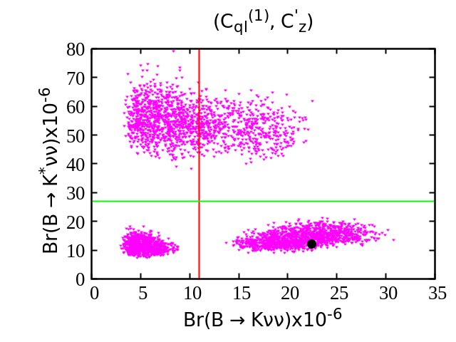
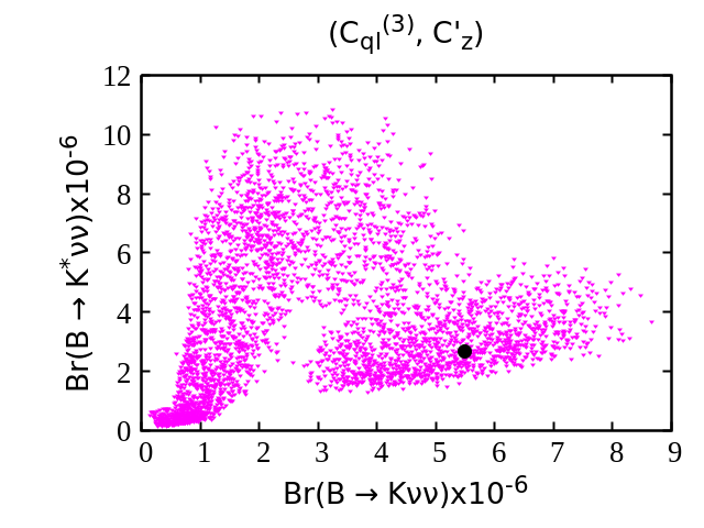
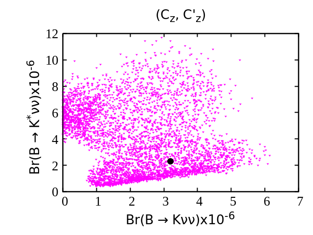
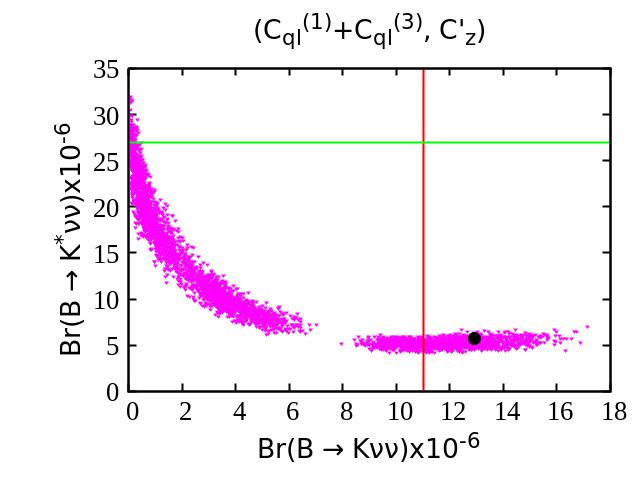
In Fig. 1, we show the allowed ranges of with few selected NP scenarios such as , , , and that best explains the data. Best fit values of are shown with a black dot in Fig. 1. The allowed range of each observable is obtained by using the allowed ranges of the NP couplings. The red and green line represents the experimental upper bound of and , respectively. It is evident that the allowed ranges of and obtained with and SMEFT scenarios are compatible with the experimental upper bound. In case of and NP scenarios, although the best fit value does not simultaneously satisfy the experimental upper bound, there still exist some NP parameter space that can, in principle, satisfy both the constraint. It is also evident that, the best fit value of obtained with NP coupling is very close to the experimental upper bound of .
III.4 Effects of SMEFT coefficients in and decay observables
Our main objective is to investigate NP effects on and decay observables in a model independent SMEFT framework. Based on our analysis and the constraint imposed by the experimental upper bound of and , we chose three NP scenarios namely, , , and that corresponds to larger PullSM value than the rest of the NP scenarios. The results are listed in Table. 9, Table. 10, Table. 11 and Table. 12, respectively. Our observations are as follows
| decay ( mode) | |||||
| SMEFT Couplings | BR | ||||
| 4.785 | 0.706 | 0.056 | 0.786 | ||
| [0.294, 14.542] | [0.051, 0.804] | [-0.276, 0.316] | [0.014, 2.100] | ||
| 3.972 | 0.477 | 0.028 | 0.539 | ||
| [0.263, 22.544] | [0.325, 0.558] | [-0.351, 0.091] | [0.008, 4.414] | ||
| 5.102 | 0.802 | 0.017 | 0.838 | ||
| [1.453, 12.108] | [0.738, 0.910] | [-0.131, 0.087] | [0.085, 1.782] | ||
| 4.921 | 0.393 | 0.001 | 0.668 | ||
| [2.085, 19.113] | [0.344, 0.528] | [-0.352, 0.201] | [0.075, 3.464] | ||
| 4.990 | 0.707 | 0.055 | 0.820 | ||
| [0.293, 14.580] | [0.048, 0.804] | [-0.277, 0.314] | [0.013, 2.124] | ||
| 4.165 | 0.476 | 0.029 | 0.565 | ||
| [0.266, 22.458] | [0.559, 0.325] | [-0.351, 0.093] | [0.008,4.397] | ||
| decay ( mode) | |||||||||
| SMEFT Couplings | bin | ||||||||
| 0.074 | 0.294 | 0.853 | 0.019 | 0.074 | 0.213 | -0.000 | -0.007 | ||
| [-0.369, 0.422] | [0.196, 0.949] | [0.525, 0.902] | [-0.092, 0.105] | [0.049, 0.237] | [0.131, 0.225] | [-0.001, 0.001] | [-0.010, 0.023] | ||
| 0.518 | 0.736 | 0.009 | 0.134 | 0.182 | 0.008 | -0.046 | 0.539 | ||
| [-0.465, 0.123] | [0.430, 0.672] | [0.661, 0.773] | [-0.119, 0.030] | [0.116, 0.170] | [0.160, 0.185] | [-0.049, 0.036] | [-0.054, 0.067] | ||
| 0.023 | 0.198 | 0.901 | 0.006 | 0.050 | 0.225 | 0.000 | -0.005 | ||
| [-0.174, 0.116] | [0.090, 0.262] | [0.869, 0.955] | [-0.044, 0.029] | [0.023, 0.066] | [0.215, 0.239] | [-0.001, 0.001] | [-0.013, 0.017] | ||
| 0.001 | 0.601 | 0.694 | 0.000 | 0.155 | 0.175 | -0.002 | -0.016 | ||
| [-0.467, 0.266] | [0.459, 0.653] | [0.670, 0.758] | [-0.119, 0.068] | [0.124, 0.166] | [0.169, 0.188] | [-0.047, 0.007] | [-0.054, 0.065] | ||
| 0.073 | 0.293 | 0.854 | 0.018 | 0.073 | 0.213 | -0.000 | -0.007 | ||
| [-0.369, 0.419] | [0.196, 0.951] | [0.524, 0.902] | [-0.092, 0.105] | [0.049, 0.238] | [0.131, 0.225] | [-0.001, 0.001] | [-0.010, 0.023] | ||
| 0.038 | 0.519 | 0.735 | 0.010 | 0.134 | 0.182 | 0.030 | -0.046 | ||
| [-0.465, 0.126] | [0.429, 0.671] | [0.661, 0.773] | [-0.119, 0.030] | [0.116, 0.170] | [0.160, 0.185] | [-0.049, 0.036] | [-0.049, 0.067] | ||
| decay ( mode) | |||||
| SMEFT Couplings | BR | ||||
| 0.628 | 0.705 | 0.070 | 0.807 | ||
| [0.076, 2.650] | [0.104, 0.896] | [-0.274, -0.274] | [0.040, 2.958] | ||
| 1.934 | 0.369 | 0.050 | 0.523 | ||
| [0.157, 10.021] | [0.278, 0.511] | [-0.403, 0.064] | [0.012, 4.074] | ||
| 0.636 | 0.829 | 0.030 | 0.817 | ||
| [0.178, 1.989] | [0.656, 0.923] | [-0.099, 0.122] | [0.116, 2.405] | ||
| 2.739 | 0.350 | 0.012 | 0.741 | ||
| [1.190, 8.196] | [0.282, 0.480] | [-0.410, 0.237] | [0.105, 3.197] | ||
| 0.652 | 0.708 | 0.068 | 0.838 | ||
| [0.076, 2.656] | [0.101, 0.896] | [-0.275, 0.246] | [0.040, 2.966] | ||
| 2.027 | 0.368 | 0.050 | 0.548 | ||
| [0.158, 10.026] | [0.278, 0.510] | [-0.403, 0.064] | [0.012, 4.120] | ||
| decay | |||||||||
| SMEFT Couplings | bin | ||||||||
| 0.046 | 0.148 | 0.426 | -0.009 | 0.018 | 0.004 | 0.018 | -0.084 | ||
| [-0.183, 0.164] | [0.052, 0.448] | [0.276, 0.474] | [-0.107, 0.119] | [-0.280, 0.062] | [-0.158, 0.027] | [-0.043, 0.067] | [-0.213, 0.207] | ||
| 0.033 | 0.315 | 0.342 | 0.023 | 0.144 | 0.072 | 0.043 | 0.000 | ||
| [-0.268, 0.043] | [0.245, 0.361] | [0.319, 0.378] | [-0.073, 0.212] | [-0.073, 0.212] | [-0.164, 0.156] | [-0.087, 0.071] | [-0.061, 0.051] | ||
| 0.020 | 0.085 | 0.457 | 0.012 | 0.023 | 0.009 | 0.020 | 0.098 | ||
| [-0.066, 0.082] | [0.172, 0.038] | [0.414, 0.481] | [-0.028, 0.049] | [-0.080, 0.066] | [-0.040, 0.030] | [-0.062, 0.099] | [-0.151, 0.145] | ||
| 0.008 | 0.325 | 0.338 | -0.132 | 0.013 | 0.006 | -0.000 | 0.197 | ||
| [-0.273, 0.158] | [0.260, 0.359] | [0.321, 0.370] | [-0.189, 0.212] | [0.212, 0.043] | [-0.081, 0.021] | [-0.060, 0.010] | [-0.200, 0.200] | ||
| 0.046 | 0.146 | 0.427 | -0.008 | 0.019 | 0.005 | 0.018 | -0.083 | ||
| [-0.183, 0.164] | [0.052, 0.052] | [0.275, 0.474] | [-0.108, 0.119] | [-0.280, 0.063] | [-0.159, 0.028] | [-0.043, 0.067] | [-0.213, 0.207] | ||
| 0.033 | 0.316 | 0.342 | 0.023 | 0.145 | 0.072 | 0.043 | -0.000 | ||
| [-0.268, 0.043] | [0.245, 0.361] | [0.319, 0.378] | [-0.072, 0.212] | [-0.164, 0.156] | [-0.082, 0.078] | [-0.061, 0.051] | [-0.177, 0.179] | ||
-
•
BR : In case of decay, branching ratio deviates from the SM prediction by in the presence of SMEFT couplings at the low region, whereas, almost deviation is observed in the presence of coupling at the high region. In case of decay channel, no significant deviation is observed at low region. However, at high region, there is more than deviation in presence of and NP couplings. Moreover, with NP coupling, the deviation from the SM prediction is quite significant and it is distinguishable from the SM prediction at more than .
-
•
: For the decay channel, deviates from the SM prediction by in the presence of NP couplings at the low region. Moreover, a significant deviation of more than is observed in the presence of and NP couplings. At the high region, deviates more than and in the presence of and NP couplings, respectively. Similarly, a deviation of more than is observed in the presence of NP coupling. In case of channel, a deviation of more than is observed with NP coupling at both low and high region.
-
•
: For the decay, a significant deviation of more than from the SM prediction is observed in all the three NP scenarios at both low and high region. For the decay channel, the deviation from the SM prediction is observed to be in the presence of and coupling in the low region, whereas, at the high region, a deviation of more than is observed in case of all the NP scenarios.
-
•
: We observe a deviation of more than and from the SM prediction in the ratio of branching fractions for the and decay channels in case all the NP scenarios at both low and high region.
-
•
: For the decay channel, the angular observable deviates from the SM prediction at more than significance in the presence of , , , and NP couplings at the low and high regions. For the decay channel, deviation from the SM prediction is observed at low region with the , and NP couplings, whereas, at high region, a deviation of more than is observed with , , and NP couplings.
-
•
: In case of decay channel, in the presence of and NP couplings the angular observable deviates from the SM prediction at more than at the low region, whereas, it deviates more than at the high region. For the decay, a deviation of more than from the SM prediction is observed at the low and the high regions with and NP couplings.
-
•
: In channel, we observe a deviation of from the SM prediction in the presence of and NP couplings at low region, whereas, it deviates more than at high region. Similarly, with coupling, we observe a deviation of more than at the high region for the decay mode.
-
•
: For the decay, we observe a deviation of more than and in case of all the NP scenarios at low and high regions, respectively. For the decay channel, no significant deviation is observed at the low region. At the high region, however, it deviates more than in case of each NP scenarios.
-
•
: A deviation of around and is observed in the presence of and couplings at the low and high regions, respectively for the decay mode. Similarly, at the low and high regions, a deviation of more than and is observed in case of each NP scenarios for the decay channel.
-
•
: In decay channel, a deviation of around from the SM prediction is observed in the presence of coupling in the low region. However, in the high region, a deviation of more than is observed in the presence of the and couplings. Similarly, for the decay channel, a deviation of more than and is observed in each NP scenarios at the low and high regions, respectively.
-
•
: For the decay channel, no significant deviation is observed in the low region. However, a deviation of more than and is observed in the presence of , and NP couplings at the high region.
-
•
: There is a deviation of more than in the low region for the decay channel in case of all the NP scenarios. Moreover, at the high region, more than deviation is observed in the presence of and couplings.
-
•
: In the low region, no significant deviation is observed in for the decay mode. However, in the high region, a deviation of more than is observed in the presence of , , and NP couplings.
-
•
: For the decay channel, a deviationof around is observed in the low region with and NP couplings. However, in the high region, deviates from the SM prediction by more than in each NP scenarios.
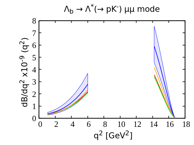
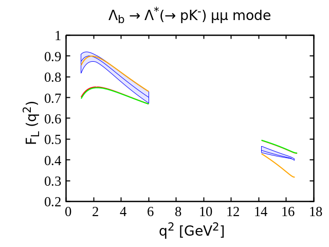
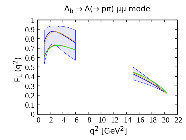
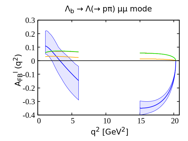
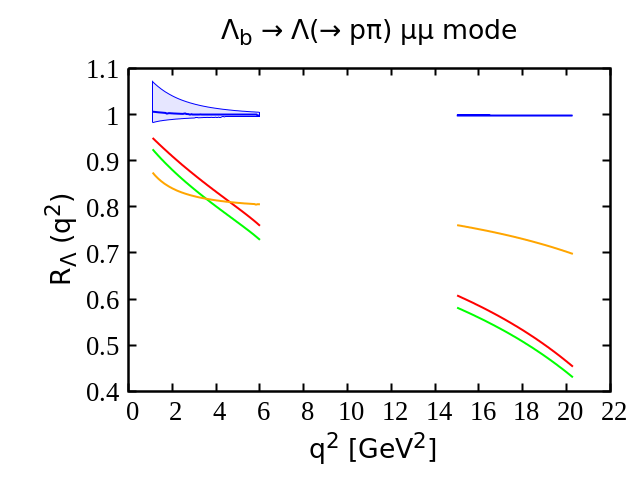
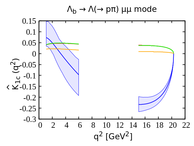
In Fig. 2 and Fig. 3, we display several dependent observables pertaining to and decay modes in the SM and in few selected NP scenarios, namely , and , respectively. The SM central line and the corresponding uncertainty band obtained at CL are shown with blue color, whereas, the effects of , and NP couplings are shown with green, orange and red color respectively. Our main observations are as follows.

-
•
: The differential branching ratio for and decays is reduced at all in case of most of the NP scenarios. In decays, the differential branching ratio is enhanced with NP coupling. All the NP scenarios are distinguishable from the SM prediction at more than in the high region. In the low region, however, it lies within the SM error band. The deviation from the SM prediction is more pronounced in case of NP scenario.
-
•
: For the decay channel, deviation in from the SM prediction is more pronounced in case of and NP scenarios in the low region. In the high region, the deviation from SM prediction is more prominent in case of and NP scenarios and they are clearly distinguishable from the SM at more than significance. In the case of decay, although a slight deviation is observed in case of NP scenario, it, however, is indistinguishable from the SM prediction.
-
•
: For the decay channel, a significantdeviation from the SM prediction is observed in in case of all the NP scenarios and they are clearly distinguishable from the SM at more than at low and high regions. In the SM, we observe the zero crossing point of at and at , respectively. With NP, there is no zero crossing of at low region. However, at the high region, we observe the zero crossing point at and with , and NP couplings, respectively. For decay, in the low region, a slight deviation in is observed with all the NP scenarios but they are indistinguishable from the SM prediction. However, at high region, the deviation observed is quite significant and all the NP scenarios are distinguishable from the SM prediction at more than . In the SM, a zero crossing point of is observed at . However, no zero crossing point is observed with NP couplings for this decay channel.
-
•
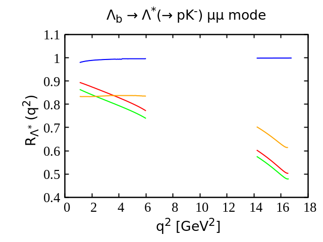
: The ratio of branching fraction shows significant deviation in case of all the NP scenarios and it is clearly distinguishable from the SM prediction at more than significance at both low and high regions.
In Fig. 4 and Fig. 5, we display the NP sensitivities of several observables for the and decay modes in the low and high regions. The SM central line and the error band is shown with blue. The green, orange and red lines correspond to NP contributions coming from the best fit values of , and NP couplings of Table. 6.
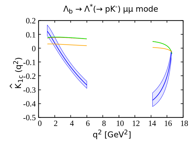
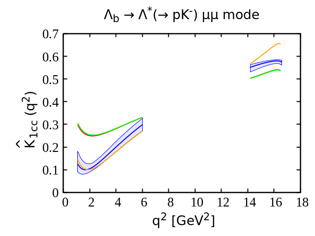
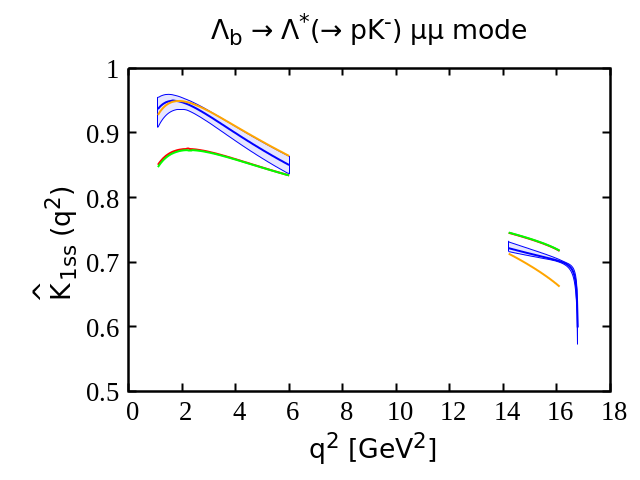
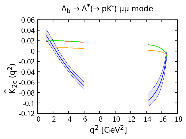
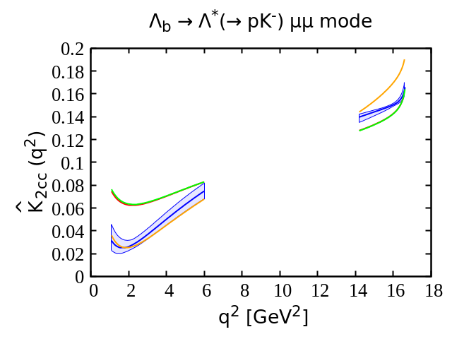
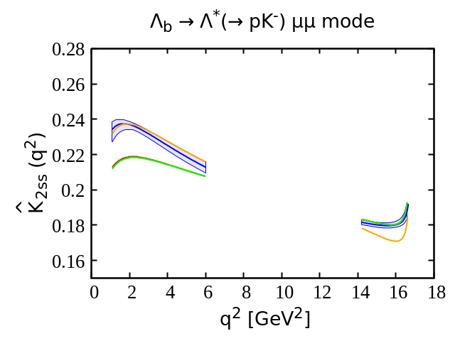
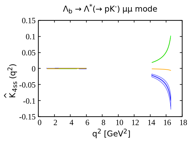
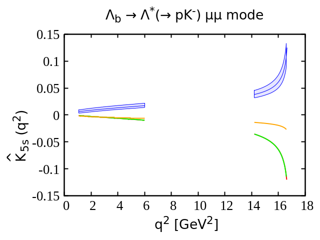
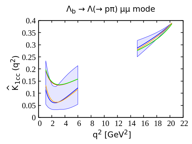
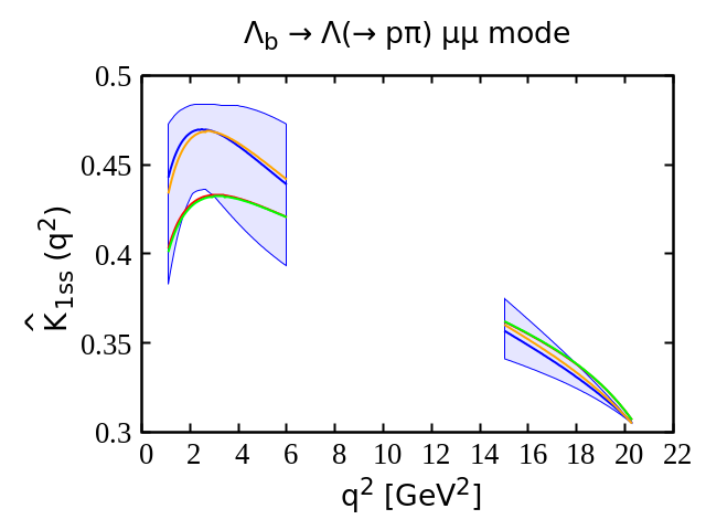
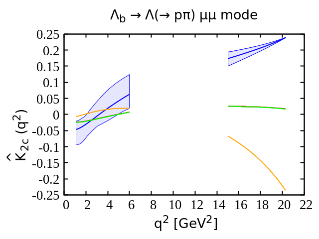
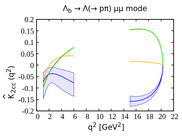
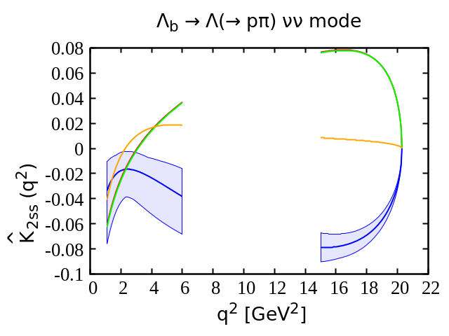
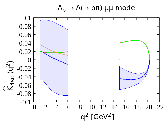
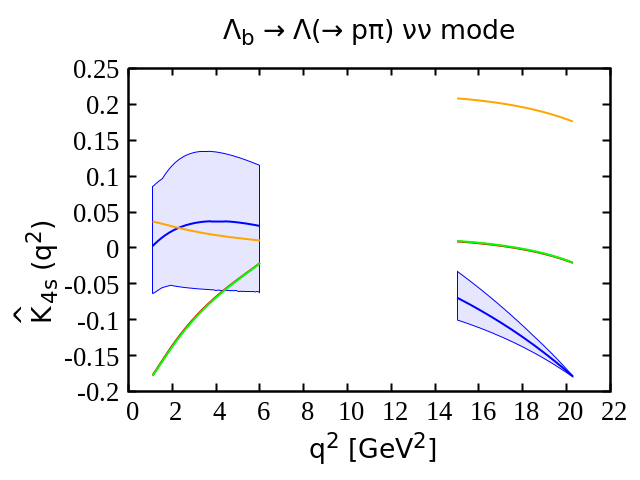
Although deviation from the SM prediction in the observables is observed in case of all the NP scenarios, it is, however, more pronounced in case of and NP scenarios. For the channel, it is observed that, irrespective of the NP contribution, the ratios , and remain independent of both short distance and long distance physics. For and the dependence on the new physics follow the same pattern as in . Similarly, for and , the dependence on the new physics follow the same pattern as in . For the channel, NP dependence of follows the same pattern as in . Similarly, for and , the NP dependence is quite similar to that of . Moreover, variation of and as a function of looks quite similar in case of decay channel. We observe that deviation from the SM prediction is more pronounced in case of and NP scenarios.
We now proceed to discuss the effects of NP in and decay observables.
III.5 Effects of SMEFT coefficients in and decay observables
Study of rare decays mediated via quark level transition can, in principle, provide complementary information regarding NP in transition decays. In this connection, we wish to explore the effects of NP in transition decays on several observables pertaining to and decay modes. We consider three NP scenarios such as , and from Table. 6 that best explain the anomalies present in the data. Effect of these NP couplings on and decay observables are listed in Table. 13.
| decay | decay | |||
| SMEFT Couplings | BR | BR | ||
| 1.205 | 0.717 | 1.007 | 0.595 | |
| [-0.001, 3.931] | [0.507, 0.731] | [0.001, 4.243] | [0.318, 0.710] | |
| 0.834 | 0.716 | 0.689 | 0.581 | |
| [0.006, 3.288] | [0.506, 0.730] | [0.000, 3.624] | [0.333, 0.721] | |
| 2.053 | 0.669 | 2.060 | 0.624 | |
| [0.006, 3.288] | [0.506, 0.730] | [1.327, 4.650] | [0.330, 0.709] | |
Our main observations are as follows.
-
•
BR : In the decay channel, branching ratio deviates more than from the SM prediction in the presence of and NP couplings. Similarly, in the decay channel, the branching ratio deviates more than in the presence of and NP couplings.
-
•
: For the decay mode, shows , and deviations from the SM prediction in the presence of , and NP couplings, respectively. Similarly, for the decay mode, shows deviations of around and from the SM prediction in presence of these NP couplings.
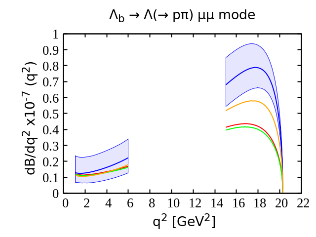
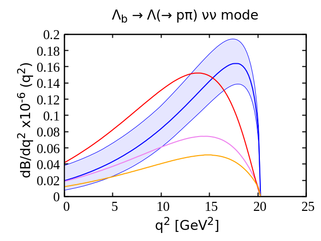
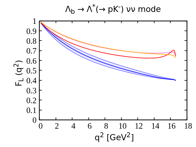
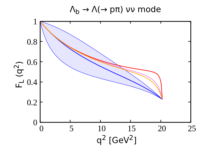
In Fig. 6, we display differential branching ratio and longitudinal polarization fraction pertaining to decay modes in the SM and in case of , and NP scenarios. The SM central line and the corresponding uncertainty band obtained at CL are shown with blue color, whereas, the effects of , and are represented by violet, orange and red color respectively. Our observations are as follows.
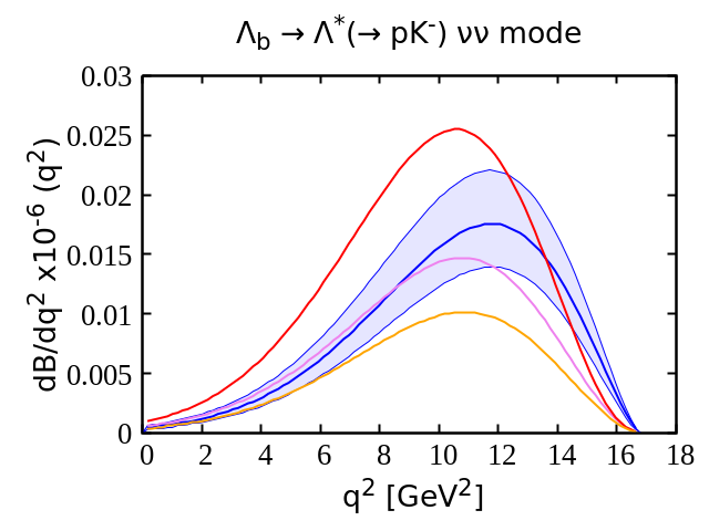
-
•
: The differential branching ratio for decays is enhanced at all below , whereas, it is reduced at the high region in case of NP scenario. With NP coupling, the differential branching ratio lies within the SM error band except at . Similarly, with NP coupling, it is reduced at all values of . The deviation from the SM prediction is more pronounced in case of and NP scenarios and they are clearly distinguishable from the SM prediction at more than . It should be noted that, in all the NP scenarios, the peak of the distribution appears at slightly lower value of than in the SM.
In case of decays, the differential branching ratio is slightly enhanced at all below whereas, it is reduced at the high region in case of NP scenario. However, it is reduced at all with and NP couplings. The deviation from the SM prediction is more pronounced in case of and NP scenarios and they are clearly distinguishable from the SM prediction at more than . Moreover, similar to decays, the peak of the distribution appears at slightly lower value of than in the SM.
-
•
: For both the decay modes, the longitudinal polarization fraction is enhanced at all in case of all the NP scenarios. The deviation from the SM prediction observed in the high region is quite significant and they are clearly distinguishable from the SM prediction at more than . The deviation from the SM prediction is more pronounced in case of NP scenario.
IV Conclusion
In light of anomalies observed in various quark-level transition decays, we perform an in-depth angular analysis of baryonic and decays mediated via and quark level transition. Our main aim of this study is to explore the connections between and quark level transition decays in a model independent way. In this context, we use the standard model effective field theory formalism with dimension six operators that can, in principle, provide correlated NP effects in these decay modes. For the form factors we use the values obtained from MCN, whereas, for the form factors, we use the recent results obtained from LQCD approach. We construct several NP scenarios based on NP contributions from single operators as well as from two different operators and try to find the scenario that best explains the anomalies present in transition decays. To find the best fit values of the SMEFT coefficients, we perform a naive analysis with the data. We include total eight measurements in our fit. It should, however, be mentioned that, in our fit, we have not included the latest measurement from LHCb. It is observed that the scenarios provide better fit to the data than the scenarios. More specifically, we get much better fit with , , , and NP scenarios. The pullSM for these scenarios are comparatively larger than any other scenarios. Next we check the compatibility of our fit results with the measured values of . It is observed that the allowed ranges of and obtained with and SMEFT scenarios are compatible with the experimental upper bound. In case of and NP scenarios, although the best fit value does not simultaneously satisfy the experimental upper bound, there still exist some NP parameter space that can, in principle, satisfy both the constraint.
A brief summary of our results are as follows.
-
•
The differential branching ratio for the and decays deviates from the SM prediction in case of all the NP scenarios and they are distinguishable from the SM prediction at more than in the high region. Similarly, deviates significantly from the SM prediction in case of all the NP scenarios. For the decay mode, the zero crossing point of at and with , and NP couplings are clearly distinguishable from the SM zero crossing point at . For the decays, although there is a zero crossing point at , no zero crossing point is observed with NP couplings for this decay channel. Moreover, the ratio of branching ratio deviates significantly from the SM prediction in case of all the NP scenarios.
-
•
In case of decay, the deviation from the SM prediction in the differential branching ratio is more pronounced in case of and NP scenarios and they are clearly distinguishable from the SM prediction at more than . In case of decays, The deviation from the SM prediction is more pronounced in case of and NP scenarios and they are clearly distinguishable from the SM prediction at more than . Similarly, deviates significantly from the SM prediction in the high region and it is clearly distinguishable from the SM prediction at more than .
Study of and mediated via and transition decays can be valuable in understanding the anomalies observed in meson decays. Our analysis can be further improved once more precise data on the form factor is available from LQCD. Moreover, more precise data on and in future, can, in principle, put severe constraint on several NP scenarios.
Acknowledgement
We would like to express our gratitude to N. Rajeev for insightful and engaging discussions related to the topic addressed in this article. We would also like to thank Diganta Das, Jaydeb Das and Stefan Meinel for their helpful exchanges regarding transition form factors.
References
- (1) R. Aaij et al., “Test of lepton universality in beauty-quark decays,” Nature Phys., vol. 18, no. 3, pp. 277–282, 2022.
- (2) R. Aaij et al., “Test of lepton universality with decays,” JHEP, vol. 08, p. 055, 2017.
- (3) R. Aaij et al., “Measurement of -Averaged Observables in the Decay,” Phys. Rev. Lett., vol. 125, no. 1, p. 011802, 2020.
- (4) A. Abdesselam et al., “Test of Lepton-Flavor Universality in Decays at Belle,” Phys. Rev. Lett., vol. 126, no. 16, p. 161801, 2021.
- (5) M. Bordone, G. Isidori, and A. Pattori, “On the Standard Model predictions for and ,” Eur. Phys. J. C, vol. 76, no. 8, p. 440, 2016.
- (6) G. Hiller and F. Kruger, “More model-independent analysis of processes,” Phys. Rev. D, vol. 69, p. 074020, 2004.
- (7) “Test of lepton universality in decays,” 12 2022.
- (8) “Measurement of lepton universality parameters in and decays,” 12 2022.
- (9) R. Aaij et al., “Measurement of Form-Factor-Independent Observables in the Decay ,” Phys. Rev. Lett., vol. 111, p. 191801, 2013.
- (10) R. Aaij et al., “Angular analysis of the decay using 3 fb-1 of integrated luminosity,” JHEP, vol. 02, p. 104, 2016.
- (11) M. Aaboud et al., “Angular analysis of decays in collisions at TeV with the ATLAS detector,” JHEP, vol. 10, p. 047, 2018.
- (12) CMS, “Measurement of the and angular parameters of the decay in proton proton collisions at = 8 TeV,” 2017.
- (13) A. Abdesselam et al., “Angular analysis of ,” in LHC Ski 2016: A First Discussion of 13 TeV Results, 4 2016.
- (14) S. Descotes-Genon, J. Matias, M. Ramon, and J. Virto, “Implications from clean observables for the binned analysis of at large recoil,” JHEP, vol. 01, p. 048, 2013.
- (15) S. Descotes-Genon, T. Hurth, J. Matias, and J. Virto, “Optimizing the basis of observables in the full kinematic range,” JHEP, vol. 05, p. 137, 2013.
- (16) S. Descotes-Genon, L. Hofer, J. Matias, and J. Virto, “On the impact of power corrections in the prediction of observables,” JHEP, vol. 12, p. 125, 2014.
- (17) R. Aaij et al., “Branching Fraction Measurements of the Rare and - Decays,” Phys. Rev. Lett., vol. 127, no. 15, p. 151801, 2021.
- (18) R. Aaij et al., “Differential branching fraction and angular analysis of the decay ,” JHEP, vol. 07, p. 084, 2013.
- (19) R. Aaij et al., “Angular analysis and differential branching fraction of the decay ,” JHEP, vol. 09, p. 179, 2015.
- (20) R. Aaij et al., “Tests of lepton universality using and decays,” Phys. Rev. Lett., vol. 128, no. 19, p. 191802, 2022.
- (21) F. Dattola, “Search for decays with an inclusive tagging method at the Belle II experiment,” in 55th Rencontres de Moriond on Electroweak Interactions and Unified Theories, 5 2021.
- (22) N. Rajeev and R. Dutta, “Consequences of b→s+- anomalies on B→K(*)¯, Bs→(,’)¯ and Bs→¯ decay observables,” Phys. Rev. D, vol. 105, no. 11, p. 115028, 2022.
- (23) M. K. Mohapatra, N. Rajeev, and R. Dutta, “Combined analysis of Bc→Ds(*)+- and Bc→Ds(*)¯ decays within Z’ and leptoquark new physics models,” Phys. Rev. D, vol. 105, no. 11, p. 115022, 2022.
- (24) Y. Li, J. Hua, and K.-C. Yang, “ Decays in a Family Non-universal Model,” Eur. Phys. J. C, vol. 71, p. 1775, 2011.
- (25) Z.-R. Huang, M. A. Paracha, I. Ahmed, and C.-D. Lü, “Testing Leptoquark and Models via Decays,” Phys. Rev. D, vol. 100, no. 5, p. 055038, 2019.
- (26) F. Falahati and A. Zahedidareshouri, “Forward-backward asymmetries of and transitions in two Higgs doublet model,” Phys. Rev. D, vol. 90, no. 7, p. 075002, 2014.
- (27) I. Ahmed, M. Ali Paracha, and M. J. Aslam, “Model Independent Analysis of the Forward-Backward Asymmetry for the Decay,” Eur. Phys. J. C, vol. 71, p. 1521, 2011.
- (28) B. Capdevila, A. Crivellin, S. Descotes-Genon, J. Matias, and J. Virto, “Patterns of New Physics in transitions in the light of recent data,” JHEP, vol. 01, p. 093, 2018.
- (29) V. Bashiry, “Lepton polarization in Decays,” JHEP, vol. 06, p. 062, 2009.
- (30) W.-F. Wang and Z.-J. Xiao, “The semileptonic decays in the perturbative QCD approach beyond the leading-order,” Phys. Rev. D, vol. 86, p. 114025, 2012.
- (31) R.-H. Li, C.-D. Lu, and W. Wang, “Branching ratios, forward-backward asymmetries and angular distributions of in the standard model and new physics scenarios,” Phys. Rev. D, vol. 83, p. 034034, 2011.
- (32) N. Rajeev, N. Sahoo, and R. Dutta, “Angular analysis of decays as a probe to lepton flavor universality violation,” Phys. Rev. D, vol. 103, no. 9, p. 095007, 2021.
- (33) T. E. Browder, N. G. Deshpande, R. Mandal, and R. Sinha, “Impact of measurements on beyond the Standard Model theories,” 7 2021.
- (34) C. Bobeth, A. J. Buras, F. Kruger, and J. Urban, “QCD corrections to , , and in the MSSM,” Nucl. Phys. B, vol. 630, pp. 87–131, 2002.
- (35) W. Altmannshofer, A. J. Buras, D. M. Straub, and M. Wick, “New strategies for New Physics search in , and decays,” JHEP, vol. 04, p. 022, 2009.
- (36) S. Descotes-Genon, S. Fajfer, J. F. Kamenik, and M. Novoa-Brunet, “Implications of anomalies for future measurements of and ,” Phys. Lett. B, vol. 809, p. 135769, 2020.
- (37) S. Fajfer, N. Košnik, and L. Vale Silva, “Footprints of leptoquarks: from to ,” Eur. Phys. J. C, vol. 78, no. 4, p. 275, 2018.
- (38) R. Aaij et al., “Test of lepton universality with decays,” JHEP, vol. 05, p. 040, 2020.
- (39) S. Meinel and G. Rendon, “ form factors from lattice QCD,” Phys. Rev. D, vol. 103, no. 7, p. 074505, 2021.
- (40) S. Meinel and G. Rendon, “c→*(1520) form factors from lattice QCD and improved analysis of the b→*(1520) and b→c*(2595,2625) form factors,” Phys. Rev. D, vol. 105, no. 5, p. 054511, 2022.
- (41) S. Descotes-Genon and M. Novoa-Brunet, “Angular analysis of the rare decay ,” JHEP, vol. 06, p. 136, 2019. [Erratum: JHEP 06, 102 (2020)].
- (42) D. Das and J. Das, “The decay at low-recoil in HQET,” JHEP, vol. 07, p. 002, 2020.
- (43) Y. Amhis, S. Descotes-Genon, C. Marin Benito, M. Novoa-Brunet, and M.-H. Schune, “Prospects for New Physics searches with decays,” Eur. Phys. J. Plus, vol. 136, no. 6, p. 614, 2021.
- (44) Y.-S. Li, S.-P. Jin, J. Gao, and X. Liu, “The transition form factors and angular distributions of the decay supported by baryon spectroscopy,” 10 2022.
- (45) W. Detmold, C. J. D. Lin, S. Meinel, and M. Wingate, “b→+- form factors and differential branching fraction from lattice QCD,” Phys. Rev. D, vol. 87, no. 7, p. 074502, 2013.
- (46) W. Detmold and S. Meinel, “ form factors, differential branching fraction, and angular observables from lattice QCD with relativistic quarks,” Phys. Rev. D, vol. 93, no. 7, p. 074501, 2016.
- (47) C.-H. Chen and C. Q. Geng, “Lepton asymmetries in heavy baryon decays of Lambda(b) — Lambda lepton+ lepton-,” Phys. Lett. B, vol. 516, pp. 327–336, 2001.
- (48) M. J. Aslam, Y.-M. Wang, and C.-D. Lu, “Exclusive semileptonic decays of Lambda(b) — Lambda l+ l- in supersymmetric theories,” Phys. Rev. D, vol. 78, p. 114032, 2008.
- (49) Y.-m. Wang, Y. Li, and C.-D. Lu, “Rare Decays of Lambda(b) — Lambda + gamma and Lambda(b) — Lambda + l+ l- in the Light-cone Sum Rules,” Eur. Phys. J. C, vol. 59, pp. 861–882, 2009.
- (50) Y.-M. Wang, Y.-L. Shen, and C.-D. Lu, “Lambda(b) — p, Lambda transition form factors from QCD light-cone sum rules,” Phys. Rev. D, vol. 80, p. 074012, 2009.
- (51) T. M. Aliev, K. Azizi, and M. Savci, “Analysis of the decay in QCD,” Phys. Rev. D, vol. 81, p. 056006, 2010.
- (52) Y.-M. Wang and Y.-L. Shen, “Perturbative Corrections to Form Factors from QCD Light-Cone Sum Rules,” JHEP, vol. 02, p. 179, 2016.
- (53) T. Gutsche, M. A. Ivanov, J. G. Korner, V. E. Lyubovitskij, and P. Santorelli, “Rare baryon decays and : differential and total rates, lepton- and hadron-side forward-backward asymmetries,” Phys. Rev. D, vol. 87, p. 074031, 2013.
- (54) L. Mott and W. Roberts, “Rare dileptonic decays of in a quark model,” Int. J. Mod. Phys. A, vol. 27, p. 1250016, 2012.
- (55) L.-L. Liu, X.-W. Kang, Z.-Y. Wang, and X.-H. Guo, “Rare decay in the Bethe-Salpeter equation approach,” Chin. Phys. C, vol. 44, no. 8, p. 083107, 2020.
- (56) T. Aaltonen et al., “Observation of the Baryonic Flavor-Changing Neutral Current Decay ,” Phys. Rev. Lett., vol. 107, p. 201802, 2011.
- (57) R. Aaij et al., “Differential branching fraction and angular analysis of decays,” JHEP, vol. 06, p. 115, 2015. [Erratum: JHEP 09, 145 (2018)].
- (58) R. Aaij et al., “Angular moments of the decay at low hadronic recoil,” JHEP, vol. 09, p. 146, 2018.
- (59) C.-S. Huang and H.-G. Yan, “Exclusive rare decays of heavy baryons to light baryons: Lambda(b) — Lambda gamma and Lambda(b) — Lambda l+ l-,” Phys. Rev. D, vol. 59, p. 114022, 1999. [Erratum: Phys.Rev.D 61, 039901 (2000)].
- (60) T. Feldmann and M. W. Y. Yip, “Form factors for transitions in the soft-collinear effective theory,” Phys. Rev. D, vol. 85, p. 014035, 2012. [Erratum: Phys.Rev.D 86, 079901 (2012)].
- (61) A. Ali, C. Hambrock, A. Y. Parkhomenko, and W. Wang, “Light-Cone Distribution Amplitudes of the Ground State Bottom Baryons in HQET,” Eur. Phys. J. C, vol. 73, no. 2, p. 2302, 2013.
- (62) G. Bell, T. Feldmann, Y.-M. Wang, and M. W. Y. Yip, “Light-Cone Distribution Amplitudes for Heavy-Quark Hadrons,” JHEP, vol. 11, p. 191, 2013.
- (63) V. M. Braun, S. E. Derkachov, and A. N. Manashov, “Integrability of the evolution equations for heavy–light baryon distribution amplitudes,” Phys. Lett. B, vol. 738, pp. 334–340, 2014.
- (64) D. Das, “Model independent New Physics analysis in decay,” Eur. Phys. J. C, vol. 78, no. 3, p. 230, 2018.
- (65) D. Das, “On the angular distribution of decay,” JHEP, vol. 07, p. 063, 2018.
- (66) S. Roy, R. Sain, and R. Sinha, “Lepton mass effects and angular observables in ,” Phys. Rev. D, vol. 96, no. 11, p. 116005, 2017.
- (67) H. Yan, “Angular distribution of the rare decay ,” 11 2019.
- (68) P. Böer, T. Feldmann, and D. van Dyk, “Angular Analysis of the Decay ,” JHEP, vol. 01, p. 155, 2015.
- (69) T. Blake and M. Kreps, “Angular distribution of polarised baryons decaying to ,” JHEP, vol. 11, p. 138, 2017.
- (70) T. Blake, S. Meinel, and D. van Dyk, “Bayesian Analysis of Wilson Coefficients using the Full Angular Distribution of Decays,” Phys. Rev. D, vol. 101, no. 3, p. 035023, 2020.
- (71) C.-H. Chen and C. Q. Geng, “Study of Lambda(b) — Lambda neutrino anti-neutrino with polarized baryons,” Phys. Rev. D, vol. 63, p. 054005, 2001.
- (72) B. B. Sirvanli, “Semileptonic Lambda(b) — Lambda neutrino anti-neutrino decay in the Leptophobic Z-prime model,” Mod. Phys. Lett. A, vol. 23, pp. 347–358, 2008.
- (73) B. Grzadkowski, M. Iskrzynski, M. Misiak, and J. Rosiek, “Dimension-Six Terms in the Standard Model Lagrangian,” JHEP, vol. 10, p. 085, 2010.
- (74) A. J. Buras, J. Girrbach-Noe, C. Niehoff, and D. M. Straub, “ decays in the Standard Model and beyond,” JHEP, vol. 02, p. 184, 2015.
- (75) R. L. Workman et al., “Review of Particle Physics,” PTEP, vol. 2022, p. 083C01, 2022.