Optimal Sensor Allocation with Multiple Linear Dispersion Processes

Abstract

This paper considers the optimal sensor allocation for estimating the emission rates of multiple sources in a two-dimensional spatial domain. Locations of potential emission sources are known (e.g., factory stacks), and the number of sources is much greater than the number of sensors that can be deployed, giving rise to the optimal sensor allocation problem. In particular, we consider linear dispersion forward models, and the optimal sensor allocation is formulated as a bilevel optimization problem. The outer problem determines the optimal sensor locations by minimizing the overall Mean Squared Error of the estimated emission rates over various wind conditions, while the inner problem solves an inverse problem that estimates the emission rates. Two algorithms, including the repeated Sample Average Approximation and the Stochastic Gradient Descent based bilevel approximation, are investigated in solving the sensor allocation problem. Convergence analysis is performed to obtain the performance guarantee, and numerical examples are presented to illustrate the proposed approach.

1 INTRODUCTION

1.1 Overview

Inverse modeling refers to the inference of unknown parameters of a physical system using observation data [15, 7, 43, 26]. Accurate inverse modeling hinges on where observation data are collected and how sensors are allocated. Among various inverse problems, source term estimation is an important class that can be found in fugitive methane gas leak source detection [22], air pollution source identification [19], nuclear source detection in an urban area [37], heat source localization [41], molecular strain identification [31], etc. Very often, the number of sensors that can be placed is far less than the number of potential emission sources (meaning that it is not possible to monitor all sources individually) [51]. This naturally gives rise to an important question: when the number of sensors is far less than the number of sources, how can sensors be optimally allocated to obtain accurate estimation of the emission rates for multiple sources?

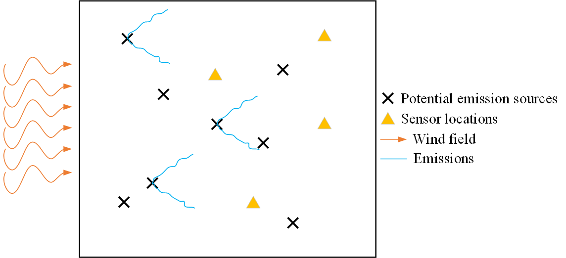
Figure 1: Illustration of the sensor allocation problem for estimating the emission rates of leaking emission sources.

To elaborate, consider an illustrative scenario in Figure 1. This figure shows seven potential emission sources where three of them are leaking under a specific wind condition. Four sensors can be afforded to detect the leaking sources by estimating their emission rates. Our objective is to determine the locations of these four sensors so that the emission rates of the seven sources can be accurately estimated. This problem can be formulated as a bilevel optimization problem: the inner level solves an inverse problem to estimate the emission rates with non-negativity constraints (on emission rates), whereas the outer level chooses the sensor locations to minimize the overall Mean Squared Error (MSE) of the estimated emission rates under various wind conditions. A nested structure can be seen, i.e., the objective function at the outer level relies on the solutions of multiple inner inverse problems.

1.2 Literature Review

Considering discrete domains, the problem of optimal sensor allocation can be formulated as a sensor selection problem [29] for which the best subset of sensor locations are chosen from a discrete set of potential candidates. The selection of sensor locations is closely related to the $D$-optimal design [20]. For example, [24] maximized the mutual information between the chosen and unselected locations, [35] used a greedy algorithm to minimize a $D$-optimal proxy of the MSE, and [48] proposes a swapping greedy algorithm to minimize the expected information gain. Due to the combinatorial nature of the sensor selection problem, convex optimization [20] and heuristics [50] have also been investigated. [2] used the $L_{0}$ regularization while casting the sensor placement for a Bayesian inverse problem as an $A$-optimal design problem. [36] used two separate optimal experimental design formulations to firstly determine the number of sensors with sparsity promoting regularizations, and then seek the optimal sensor locations using a relaxed interior point method.

For continuous domains, [6] augmented the grid-based sensor allocation with continuous variables to allow off-grid sensor placement. [17, 16] developed gradient-based stochastic optimization methods to maximize the expected information gain while approximating the forward models with polynomial chaos expansion. [39] presented a continuous-time, two-timescale stochastic gradient descent algorithm for minimizing the MSE of the hidden state estimates. [3] proposed three efficient ways of evaluating the $D$-optimal and its gradient for infinite-dimensional Bayesian linear inverse problems. Note that, the continuous-domain design problem can sometimes be converted to a discrete-domain design problem by discretizing the continuous domain and leveraging the existing algorithms and open-source tools for discrete problems, such as the ‘Chama’ software for sensor placement optimization using impact metrics [23], the ‘Polire’ software for spatial interpolation and sensor placement [32], the ‘PySensors’ software for selecting and placing a sparse set of sensors for classification and signal reconstruction [8, 5, 28].

In this paper, the sensor allocation problem is formulated as a bilevel optimization where the outer level depends on the estimated emission rates from the inner inverse problem [10, 45]. The inner problem is often an ill-posed non-smooth minimization problem. To handle the ill-posed inverse model, constraints or regularizations are often added, e.g., the tightly coupled sets of variables [14], the $L_{1}$-type prior [46], the goal-oriented inversions [42, 48], the total variation regularization [40] and the fractional Laplacian [4]. One of the most commonly adopted approaches is to add the Tikhonov regularization [47, 44, 11]. For linear inverse problems with a squared loss function, adding the Tikhonov regularization yields a closed-form $A$-optimal design [44, 12, 13]. On the other hand, when non-negativity constraints are added to emission rates and an elastic-net regularization is considered in the inverse model (as is the case in this paper), neither the closed-form design (i.e., the outer problem) nor the closed-form solution of the inverse model (i.e., the inner problem) is available [26, 52, 49]. In this case, one approach for solving bilevel optimization problems is to replace the inner problem with its necessary and sufficient Karush-Kuhn-Tucker (KKT) conditions [27]. Because this approach may not be scalable for large-scale inner problems [9], iterative algorithms are needed for solving the bilevel optimization problem, such as the stochastic approximation methods with finite-time convergence analysis under different convexity assumptions on the outer objective function [9], the bilevel stochastic gradient method with lower level constraints for large-scale problems [10], the implicit gradient-type algorithm for strongly convex linear inequality constrained lower-level problems [45, 21], and a relaxed interior point method with the Tikhonov-regularized linear inversion estimate [36].

1.3 Contributions

First, this paper presents a bilevel optimization framework for sensor placement that minimizes the MSE of the estimated emission rates, while taking into account the non-negativity of emission rates, uncertainty associated with wind conditions, and the sparsity of the inner inverse problem. Hence, for our sensor allocation problem, neither the closed-form design nor the closed-form inverse estimator is available. To the best of our knowledge, there exists no prior work that explicitly tackles the constrained non-smooth bilevel optimization for solving the optimal sensor placement problem with constrained and elastic-net regularized inversion estimators. Second, we investigate two stochastic optimization algorithms for solving the constrained non-smooth bilevel optimization problems, and obtain the performance guarantee through convergence analysis. Third, because the bilevel optimization problem is non-convex for our problem, the solution of a first-order algorithm strongly depends on the choice of the initial design. Hence, this paper also provides a practical approach to find appropriate starting points for the stochastic optimization algorithms, and demonstrate the performance of the proposed approach through comprehensive numerical experiments.

The remainder of this paper is organized as follows. Section 2 presents the inverse modeling and the bilevel optimization problem. Section 3 investigates two optimization algorithms for solving the proposed bilevel optimization problem, and presents the convergence analysis. Two numerical examples, including a simple illustrative example and a more realistic case, are presented in Section 4 to demonstrate the performance of the proposed approach. Conclusions and discussions on future research are presented in Section 5. All proofs and lengthy derivations are provided in the Appendices submitted as supplementary materials.

2 Formulation of the Optimal Sensor Allocation Problem

Let $\Omega\subset\mathbb{R}^{2}$ be a two-dimensional rectangular spatial domain. Within $\Omega$, there exist $N_{p}$ potential emission sources with known locations but unknown emission rates. Let $\theta_{i}\geq 0$ be the emission rate for the $i$th source, and let $\bm{\theta}=(\theta_{1},...,\theta_{N_{p}})$. Each source has a constant background emission rate $\mu$ under normal operation, whereas a higher-than-normal emission rate under abnormal conditions. We are interested in finding the optimal allocations of $n$ sensors that facilitate the detection of abnormal emission sources. In particular, we assume a steady concentration field, while the sources only have two states: constant leaking (i.e., constant emission rates) or not leaking (i.e., a constant background emission rate).

Note that we consider the case when the number of sensors is less than (usually far less than) the number of potential sources, i.e., $n<N_{p}$, giving rise to the optimal sensor allocation problem. When $n\geq N_{p}$, the problem becomes trivial as one could allocate at least one sensor to each emission source. Without loss of generality, the background emission rate $\mu$ is set to zero throughout this paper.

The observation model is given as follows,

(1) $$\begin{split}\bm{\Phi}=G(\bm{\theta},\bm{\beta},\bm{s})+\bm{\epsilon},\quad\bm{\epsilon}\sim\mathcal{N}(\bm{0},\bm{\Gamma}_{\epsilon}),\end{split}$$

where $\bm{\Phi}\in\mathbb{R}^{n}$ is a vector that contains the observations from $n$ sensors, $G$ is a forward dispersion model, $\bm{\beta}\in\mathbb{R}^{2}$ is the wind vector, $\bm{s}=(\bm{s}_{1},\bm{s}_{2},...,\bm{s}_{n})$ is the location of $n$ sensors with $\bm{s}_{i}=(X_{i},Y_{i})$, and $\bm{\epsilon}\sim\mathcal{N}(\bm{0},\bm{\Gamma}_{\epsilon})$ is the observation noise with $\bm{\Gamma}_{\epsilon}=\sigma^{2}_{\epsilon}\bm{I}$.

In this paper, $\bm{s}$ is the decision variable and the decision space is defined by $\Omega^{s}=\{\bm{s}\in\Omega:\bm{s}_{L}\leq\bm{s}\leq\bm{s}_{H}\}$, where $\bm{s}_{L}$ and $\bm{s}_{H}$ respectively represent the lower and upper bounds within which sensors can be placed. Given the estimated emission rates, $\hat{\bm{\theta}}(\bm{\Phi},\bm{\beta},\bm{s})$, for all $N_{p}$ sources, finding $\bm{s}$ can be formulated as minimizing the MSE averaged over various wind and emission scenarios

(2) $$\begin{split}\Psi(\bm{s})&=\mathbb{E}_{\bm{\theta},\bm{\beta}}\{\mathbb{E}_{\bm{\Phi}|\bm{\theta},\bm{\beta}}\{\|\hat{\bm{\theta}}(\bm{\Phi},\bm{\beta},\bm{s})-\bm{\theta}\|^{2}_{2}\}\}\\ &=\iiint\|\hat{\bm{\theta}}(\bm{\Phi},\bm{\beta},\bm{s})-\bm{\theta}\|^{2}_{2}\cdot p(\bm{\Phi}|\bm{\theta},\bm{\beta},\bm{s})p(\bm{\theta})p(\bm{\beta})d\bm{\Phi}d\bm{\theta}d\bm{\beta},\end{split}$$

where $p(\bm{\beta})$ and $p(\bm{\theta})$ are the prior distributions of $\bm{\beta}$ and $\bm{\theta}$. Prior knowledge on $\bm{\beta}$ can be obtained from historical data or numerical weather predictions, while prior knowledge on $\bm{\theta}$ can be elicited from domain experts on possible leaking scenarios.

The objective function (2) can be approximated from $N$ Monte Carlo samples, $\bm{\theta}^{(i)}\sim p(\bm{\theta})$, $\bm{\beta}^{(i)}\sim p(\bm{\beta})$, and $\bm{\Phi}^{(i)}\sim p(\bm{\Phi}|\bm{\theta}^{(i)},\bm{\beta}^{(i)},\bm{s})$ for $i=1,2,\cdots,N$, as follows

(3) $$\hat{\Psi}_{N}(\bm{s})=\frac{1}{N}\sum_{i=1}^{N}\|\hat{\bm{\theta}}^{(i)}(\bm{s})-\bm{\theta}^{(i)}\|^{2}_{2}$$

where $\hat{\bm{\theta}}^{(i)}(\bm{s})$ is the estimated $\bm{\theta}$ from $\bm{\Phi}^{(i)}$ given $\bm{s}$. Hence, the evaluation of (3) requires estimating the emission rate $\bm{\theta}^{(i)}$ from data (i.e., solving the inverse model first). In this paper, we obtain $\hat{\bm{\theta}}^{(i)}$ by minimizing an elastic net loss function [18],

(4) $$L(\bm{\theta})=\frac{1}{2}\|G(\bm{\theta},\bm{\beta}^{(i)},\bm{s})-\bm{\Phi}^{(i)}\|^{2}_{\bm{\Gamma}_{\epsilon}}+\lambda_{1}\|\bm{\theta}\|^{2}_{2}+\lambda_{2}\|\bm{\theta}\|_{1}\text{ s.t. }\bm{\theta}\geq\bm{0},$$

where $\|\bm{x}\|^{2}_{\bm{\Gamma}_{\epsilon}}=\sigma^{-2}_{\epsilon}\bm{x}^{T}\bm{x}$ for some vector $\bm{x}$, and $\lambda_{1}$ and $\lambda_{2}$ are the hyperparameters.

It is noted that the minimization of (4) yields the Maximum a Posteriori (MAP) estimate given a prior distribution, $p(\bm{\theta};\lambda_{1},\lambda_{2})\propto\exp(-\lambda_{1}\|\bm{\theta}\|^{2}_{2}-\lambda_{2}\|\bm{\theta}\|_{1})$ for $\bm{\theta}\geq\bm{0}$ [36]. Because emission rates are non-negative, this prior distribution incorporates the truncated Gaussian when $\lambda_{2}=0$. It also incorporates a truncated Laplacian when $\lambda_{1}=0$ so that the prior information on $\bm{\theta}$ can be flexibly captured. The posterior distribution is given by

(5) $$\begin{split}p(\bm{\theta}|\bm{\Phi}^{(i)},\bm{\beta}^{(i)},\bm{s})&\propto p(\bm{\Phi}^{(i)}|\bm{\theta},\bm{\beta}^{(i)},\bm{s})\cdot p(\bm{\theta}|\bm{\beta}^{(i)},\bm{s})\\ &=p(\bm{\Phi}^{(i)}|\bm{\theta},\bm{\beta}^{(i)},\bm{s})\cdot p(\bm{\theta}).\end{split}$$

Because $\text{log}(p(\bm{\theta}))=c-\lambda_{1}\|\bm{\theta}\|^{2}_{2}-\lambda_{2}\|\bm{\theta}\|_{1}$ for $\bm{\theta}\geq\bm{0}$ where $c$ is a constant, the MAP estimate is obtained by maximizing

(6) $$-\frac{1}{2}\|G(\bm{\theta},\bm{\beta}^{(i)},\bm{s})-\bm{\Phi}^{(i)}(\bm{s})\|^{2}_{\bm{\Gamma}_{\epsilon}}-\lambda_{1}\|\bm{\theta}\|^{2}_{2}-\lambda_{2}\|\bm{\theta}\|_{1}\textrm{ s.t. }\bm{\theta}\geq\bm{0},$$

which is a constrained non-smooth optimization problem.

In this paper, we focus on a linear dispersion model, which includes the Gaussian plume model [43] derived from the advection-diffusion equation. Confining our focus gives $G(\bm{\theta},\bm{\beta},\bm{s})=\mathcal{F}(\bm{\beta},\bm{s})\bm{\theta}$, where $\mathcal{F}(\bm{\beta},\bm{s})$ is a function of the wind vector $\bm{\beta}$ and sensor location $\bm{s}$. From (3) and (6), the problem in (2) can be cast as a bilevel optimization problem

(7a) $$\min_{\bm{s}\in\Omega^{s}}\hat{\Psi}_{N}(\bm{s})$$

(7b) $$\text{s.t.}~{}\hat{\bm{\theta}}^{(i)}(\bm{s})=\underset{\bm{\theta}}{\text{argmin}}\Big{\{}\frac{1}{2}\|\mathcal{F}(\bm{\beta}^{(i)},\bm{s})\bm{\theta}- \bm{\Phi}^{(i)}\|^{2}_{\bm{\Gamma}_{\epsilon}}+\lambda_{1}\|\bm{\theta}\|^{2}_{2}+\lambda_{2}\|\bm{\theta}\|_{1}:\bm{\theta}\geq\bm{0}\Big{\}},$$

(7c) $$\text{ for }i=0,\cdots,N-1,$$

where the evaluation of the outer objective requires the solution of the inner inverse model. Note that, the inverse problem (7b) is a convex Quadratic Programming (QP) problem:

(8) $$\hat{\bm{\theta}}^{(i)}(\bm{s})=\underset{\bm{\theta}}{\text{argmin}}\Big{\{}\frac{1}{2}\bm{\theta}^{T}\bm{C}^{(i)}\bm{\theta}+\bm{d}^{(i)}\bm{\theta}:\bm{\theta}\geq\bm{0}\Big{\}},$$

where $\bm{C}^{(i)}:=\bm{C}^{(i)}(\bm{s})=\sigma^{-2}_{\epsilon}\mathcal{F}^{*}(\bm{\beta}^{(i)},\bm{s})\mathcal{F}(\bm{\beta}^{(i)},\bm{s})+\lambda_{1}\bm{I}$ is a $N_{p}\times N_{p}$ matrix, $\bm{d}^{(i)}:=\bm{d}^{(i)}(\bm{s})=\lambda_{2}\bm{1}-\sigma^{-2}_{\epsilon}(\bm{\Phi}^{(i)}(\bm{s}))^{T}\mathcal{F}(\bm{\beta}^{(i)},\bm{s})$ is a $1\times N_{p}$ row vector, $\mathcal{F}^{*}$ is the complex conjugate transpose, and $\bm{1}$ is a $N_{p}$-dimensional row vector of ones.

3 Solving the Sensor Allocation Problem

The computational cost of the bilevel optimization problem (7) is non-trivial when $N$ is large. This section investigates two algorithms, including the repeated Sample Average Approximation (rSAA) and the Stochastic Gradient Descent based bilevel approximation (SBA), that can be used to find the optimal sensor allocation.

The rSAA algorithm, shown in Algorithm 1, involves $K$ parallel runs for $k=0,1,\cdots,K-1$. Each run solves both the outer and inner optimization problems of the bilevel optimization using only a small number of $\tilde{N}$ Monte Carlo samples to speed up the computation ($\tilde{N}\ll N$). The outputs from the $K$ repeated runs are later combined to obtain the final solution.

The algorithm starts with two initialization settings: i) the initial sensor locations, $\{\tilde{\bm{s}}^{k}_{\tilde{N},0}\in\Omega^{s}\}_{k=0}^{K-1}$, for the $K$ repeated runs, where the first subscript $\tilde{N}$ is the number of Monte Carlo samples, the second subscript is the index of the outer iteration (“0” corresponds to the initial value), and $k$ is the index of the repeated runs. (ii) $\{\hat{\bm{\theta}}_{m,0}^{(i)}\in\mathbb{R}^{+},\hat{\bm{\eta}}_{m,0}^{(i)}\in\mathbb{R}^{+}\}_{i=0,\cdots,\tilde{N}-1;m=0,\cdots,M-1}$ are the initial emission rates and the Lagrangian multipliers. For the $k$th run ($k=1,2,\cdots,K$), both outer and inner problems are solved. The outer optimization requires $M$ iterations ($m=0,1,\cdots,M-1$), and each outer iteration involves $\tilde{N}$ inner problems ($i=0,1,\cdots,\tilde{N}-1$). Each inner problem requires $J$ iterations ($j=0,1,\cdots,J-1$) to update the estimated emission rate $\hat{\bm{\theta}}_{m,j+1}^{(i)}$ and its Lagrangian multiplier $\hat{\bm{\eta}}_{m,j+1}^{(i)}$ (see Section 3.1). Once the inner problem has been solved, each outer iteration updates the sensor locations $\tilde{\bm{s}}^{k}_{\tilde{N},m+1}\leftarrow\tilde{\bm{s}}^{k}_{\tilde{N},m}$ (see Section 3.2). After the $M$ outer iterations, the optimal sensor location $\hat{\bm{s}}^{k}_{\tilde{N}}:=\tilde{\bm{s}}^{k}_{\tilde{N},M}$ is found and the objective function $\hat{\Psi}^{k}_{\tilde{N}}:=\hat{\Psi}_{\tilde{N}}(\hat{\bm{s}}^{k}_{\tilde{N},M})$ is evaluated for the $k$-th run. After the $K$ repeated runs, the final optimal sensor location $\hat{\bm{s}}_{\tilde{N}}$ is determined from $\hat{\bm{s}}^{0}_{\tilde{N}},\hat{\bm{s}}^{1}_{\tilde{N}},...,\hat{\bm{s}}^{K-1}_{\tilde{N}}$ (see Section 3.2).

Initialization $\{\tilde{\bm{s}}^{k}_{\tilde{N},0}\in\Omega^{s}\}_{k=0}^{K-1}$, $\{\hat{\bm{\theta}}_{m,0}^{(i)}\in\mathbb{R}^{+},\hat{\bm{\eta}}_{m,0}^{(i)}\in\mathbb{R}^{+}\}_{i=0,\cdots,\tilde{N}-1;m=0,\cdots,M-1}$, and a relatively small $\tilde{N}$

for $k=0,1,\cdots,K-1$ do // $K$ repeated runs

       Sample{$\bm{\theta}^{(i)},\bm{\beta}^{(i)},\bm{\Phi}^{(i)}\}_{i=1,\cdots,\tilde{N}}$

      for $m=0,1,\cdots,M-1$ do // outer problem

             for $i=0,1,\cdots,\tilde{N}-1$ do

                    for $j=0,1,\cdots,J-1$ do // inner problem

                         Update $\hat{\bm{\theta}}_{m,j+1}^{(i)}\leftarrow\hat{\bm{\theta}}_{m,j}^{(i)},\hat{\bm{\eta}}_{m,j}^{(i)}$ (see Section 3.1)

                        Update $\hat{\bm{\eta}}_{m,j+1}^{(i)}\leftarrow\hat{\bm{\theta}}_{m,j}^{(i)},\hat{\bm{\eta}}_{m,j}^{(i)}$ (see Section 3.1)

                   end for

                  

             end for

            Update $\tilde{\bm{s}}^{k}_{\tilde{N},m+1}\leftarrow\tilde{\bm{s}}^{k}_{\tilde{N},m}$ (see Section 3.2)

       end for

      Save $\hat{\bm{s}}^{k}_{\tilde{N}}:=\tilde{\bm{s}}^{k}_{\tilde{N},M}$, $\hat{\Psi}^{k}_{\tilde{N}}:=\hat{\Psi}_{\tilde{N}}(\hat{\bm{s}}^{k}_{\tilde{N},M})$

end for

Set $\hat{\bm{s}}_{\tilde{N}}=g(\hat{\bm{s}}^{0}_{\tilde{N}},\hat{\bm{s}}^{1}_{\tilde{N}},\ldots,\hat{\bm{s}}^{K-1}_{\tilde{N}})$ (see Section 3.2) // final output

Return $\hat{\bm{s}}_{\tilde{N}}$

Algorithm 1 Repeated SAA (rSAA) for Sensor Allocation Problem

To ensure $K$ is sufficiently large, the stochastic upper bound of the optimality gap can be defined as follows:

(9) $$\delta(K):=\Psi(\hat{\bm{s}}_{\tilde{N}})-\Psi^{*},$$

where $\Psi(\hat{\bm{s}}_{\tilde{N}})$ is the value of the objective function given $\hat{\bm{s}}_{\tilde{N}}$, and $\Psi^{*}$ is the true optimal value [38]. In (9), $\Psi(\hat{\bm{s}}_{\tilde{N}})$ can be estimated from $N$ Monte Carlo samples, and an approximate $100(1-\alpha)\%$ confidence upper bound for $\Psi(\hat{\bm{s}}_{\tilde{N}})$ is given by $\hat{\Psi}_{N}+z_{\alpha}\hat{\sigma}_{N}$, where $\hat{\Psi}_{N}(\hat{\bm{s}}_{\tilde{N}})=\frac{1}{N}\sum_{i=0}^{N-1}\hat{\Psi}^{(i)}(\hat{\bm{s}}_{\tilde{N}})$, $z_{\alpha}$ is the critical value from standard normal, and $\hat{\sigma}^{2}_{N}=\frac{1}{N(N-1)}\sum_{i=0}^{N-1}(\hat{\Psi}^{(i)}(\hat{\bm{s}}_{\tilde{N}})-\hat{\Psi}_{N})^{2}$. To derive the lower bound of $\Psi^{*}$, note that $\Psi^{*}\geq\mathbb{E}(\hat{\Psi}^{k}_{\tilde{N}})$ (see [38]), and an approximate $100(1-\alpha)\%$ lower bound for $\mathbb{E}(\hat{\Psi}^{k}_{\tilde{N}})$ is $\bar{\Psi}_{\tilde{N}}-t_{\alpha}\hat{\sigma}_{\tilde{N},K}$, where $\bar{\Psi}_{\tilde{N}}=\frac{1}{K}\sum_{k=0}^{K-1}\hat{\Psi}^{k}_{\tilde{N}}$, $t_{\alpha}$ is a critical value, and $\hat{\sigma}^{2}_{\tilde{N},K}=\frac{1}{K(K-1)}\sum_{k=0}^{K-1}(\hat{\Psi}^{k}_{\tilde{N}}-\bar{\Psi}_{\tilde{N}})^{2}$. Hence, for a chosen $K$, a stochastic upper bound (with confidence at least $1-2\alpha$) of $\delta(K)$ is

(10) $$\Delta(K)=(\hat{\Psi}_{N}+z_{\alpha}\hat{\sigma}_{N})-(\bar{\Psi}_{\tilde{N}}-t_{\alpha}\hat{\sigma}_{\tilde{N},K}).$$

The second algorithm, i.e., the SBA algorithm, is provided in Algorithm 2. While the SBA algorithm shares some common building blocks with the rSAA algorithm, this algorithm requires only one run. Hence, no extra steps are needed for post-processing the optimal solutions from repeated runs. In addition, following the idea of stochastic approximation [33], the $\tilde{N}$ Monte Carlo samplings $\{\bm{\theta}^{(i)},\bm{\beta}^{(i)},\bm{\Phi}^{(i)}\}_{i=1,\cdots,\tilde{N}}$ are re-sampled for each outer iteration $m$.

Initialization $\tilde{\bm{s}}_{\tilde{N},0}\in\Omega^{s}$, $\{\hat{\bm{\theta}}_{m,0}^{(i)}\in\mathbb{R}^{+},\hat{\bm{\eta}}_{m,0}^{(i)}\in\mathbb{R}^{+}\}_{i=0,\cdots,\tilde{N}-1;m=0,\cdots,M-1}$, and the small $\tilde{N}$

for $m=0,1,\cdots,M-1$ do // outer problem

       Sample {$\bm{\theta}^{(i)},\bm{\beta}^{(i)},\bm{\Phi}^{(i)}\}_{i=1,\cdots,\tilde{N}}$

       for $i=0,1,\cdots,\tilde{N}-1$ do // inner problem

             for $j=0,1,\cdots,J-1$ do

                   Update $\hat{\bm{\theta}}_{m,j+1}^{(i)}\leftarrow\hat{\bm{\theta}}_{m,j}^{(i)},\hat{\bm{\eta}}_{m,j}^{(i)}$ (see Section 3.1)

                  Update $\hat{\bm{\eta}}_{m,j+1}^{(i)}\leftarrow\hat{\bm{\theta}}_{m,j}^{(i)},\hat{\bm{\eta}}_{m,j}^{(i)}$ (see Section 3.1)

             end for

            

       end for

      Update $\tilde{\bm{s}}_{\tilde{N},m+1}\leftarrow\tilde{\bm{s}}_{\tilde{N},m}$ (see Section 3.2)

      Set $\hat{\bm{s}}_{\tilde{N}}:=\tilde{\bm{s}}_{\tilde{N},M}$ // final output

end for

Return $\hat{\bm{s}}_{\tilde{N}}$

Algorithm 2 The SGD-based Bilevel Approximation Method (SBA)

Next, we present the details of how $\hat{\bm{\theta}}_{m,j+1}^{(i)}$, $\hat{\bm{\eta}}_{m,j+1}^{(i)}$, and $\tilde{\bm{s}}_{\tilde{N},m+1}$ are updated in the inner and outer iterations for both Algorithms 3.1 and 3.2.

3.1 Update $\hat{\bm{\theta}}_{m,j+1}^{(i)}$ and $\hat{\bm{\eta}}_{m,j+1}^{(i)}$

When solving the inner problem, both algorithms require the update of $\hat{\bm{\theta}}_{m,j+1}^{(i)}$ and $\hat{\bm{\eta}}_{m,j+1}^{(i)}$. For any $i=0,1,\cdots,\tilde{N}-1$, the Lagrangian of the inner problem is given by

(11) $$\begin{split}h(\bm{s},\bm{\theta},\bm{\eta})=\frac{1}{2}\bm{\theta}^{T}\bm{C}^{(i)}\bm{\theta}+\bm{d}^{(i)}\bm{\theta}-\bm{\eta}^{T}\bm{\theta}\end{split}$$

with the KKT conditions $\bm{C}^{(i)}\bm{\theta}+(\bm{d}^{(i)})^{T}-\bm{\eta}=\bm{0}$, $\bm{\theta},\bm{\eta}\geq\bm{0}$, and $\bm{\eta}\bm{\theta}=\bm{0}$. The augmented primal-dual gradient algorithm can be employed to solve the inner QP problem by defining the augmented Lagrangian as [30]:

(12) $$h_{\gamma}(\bm{s},\bm{\theta},\bm{\eta})=\frac{1}{2}\bm{\theta}^{T}\bm{C}^{(i)}\bm{\theta}+\bm{d}^{(i)}\bm{\theta}+\sum_{b=1}^{N_{p}}\frac{[\gamma(-\theta_{b})+\eta_{b}]_{+}^{2}-\eta_{b}^{2}}{2\gamma},$$

where $\gamma$ is a penalty parameter, $\theta_{b}$ the $b$th entry of $\bm{\theta}$, and $\eta_{b}$ the $b$th entry of $\bm{\eta}$.

The gradient of the augmented Lagrangian with respect to $\bm{\theta}$ and $\bm{\eta}$ can be obtained as

(13) $$\begin{split}\nabla_{\bm{\theta}}h_{\gamma}(\bm{s},\bm{\theta},\bm{\eta})&=\bm{C}^{(i)}\bm{\theta}+(\bm{d}^{(i)})^{T}-\sum_{b=1}^{N_{p}}[\gamma(-\theta_{b})+\eta_{b}]_{+}\bm{e}_{b}^{T}\\ \nabla_{\bm{\eta}}h_{\gamma}(\bm{s},\bm{\theta},\bm{\eta})&=\sum_{b=1}^{N_{p}}\frac{1}{\gamma}([\gamma(-\theta_{b})+\eta_{b}]_{+}-\eta_{b})\bm{e}_{b}^{T}\end{split}$$

where $\bm{e}_{b}$ is an $N_{p}$-dimensional row vector with the $b$th entry being 1 and other elements being 0. Finally, $\hat{\bm{\theta}}_{m,j+1}^{(i)}$ and $\hat{\bm{\eta}}_{m,j+1}^{(i)}$ are updated as

(14) $$\begin{split}&\hat{\bm{\theta}}_{m,j+1}^{(i)}=[\hat{\bm{\theta}}_{m,j}^{(i)}-\tau_{m,j}\nabla_{\bm{\theta}}h_{\gamma}(\tilde{\bm{s}}_{\tilde{N},m},\hat{\bm{\theta}}_{m,j}^{(i)},\hat{\bm{\eta}}_{m,j}^{(i)})]_{+}\\ &\hat{\bm{\eta}}_{m,j+1}^{(i)}=[\hat{\bm{\eta}}_{m,j}^{(i)}+\tau_{m,j}\nabla_{\bm{\eta}}h_{\gamma}(\tilde{\bm{s}}_{\tilde{N},m},\hat{\bm{\theta}}_{m,j}^{(i)},\hat{\bm{\eta}}_{m,j}^{(i)})]_{+}\end{split}$$

where $\tau_{m,j}$ is the stepsize, and $[x]_{+}=x$ if $x\geq 0$ and $[x]_{+}=0$ if $x<0$.

3.2 Update $\tilde{\bm{s}}_{\tilde{N},m+1}$

The outer problem requires updating the sensor locations $\bm{s}$ given the solution of the inner problem. Since the true optimal solution may not be found for each of the $N$ inner problems (see (7b)), we approximate the gradient of $\bm{s}$ for any inner problem $i$ ($i=0,1,\cdots,N-1$) by

(15) $$\nabla_{\bm{s}}\hat{\Psi}_{\tilde{N},m}(\bm{s})=\frac{2}{\tilde{N}}\sum_{i=1}^{\tilde{N}}(\nabla_{\bm{s}}\hat{\bm{\theta}}^{(i)})^{T}(\hat{\bm{\theta}}^{(i)}-\bm{\theta}^{(i)})$$

where $\nabla_{\bm{s}}\hat{\bm{\theta}}^{(i)}$ is from the implicit differentiation of the inner optimality condition given by

(16) $$\begin{split}\nabla_{\bm{s}}\bm{\theta}&\approx(\bm{C}^{(i)})^{-1}(-\nabla_{\bm{s}}(\bm{C}^{(i)})\bm{\theta}-\nabla_{\bm{s}}(\bm{d}^{(i)})^{T}+\bm{\bar{I}}^{T}\nabla_{\bm{s}}\bm{\bar{\eta}})\\ \nabla_{\bm{s}}\bm{\bar{\eta}}&\approx(\bm{\bar{I}}(\bm{C^{(i)}})^{-1}\bm{\bar{I}}^{T})^{-1}(\bm{\bar{I}}(\bm{C^{(i)}})^{-1}(\nabla_{\bm{s}}(\bm{C}^{(i)})\bm{\theta}+\nabla_{\bm{s}}(\bm{d}^{(i)})^{T})).\end{split}$$

Here, let $\{j;\theta^{(i)}_{j}=0\}$ be a set of active constraints, $\bm{\bar{I}}$ contains the rows of an identity matrix $\bm{I}$ corresponding to the active constraints, and $\bm{\bar{\eta}}$ denotes the elements of $\bm{\eta}$ that correspond to the active constraints.

Next, we show how (16) is derived. Following the idea of [34, 45], the Lagrangian function of the inner QP problem can be written as

(17) $$h(\bm{s},\bm{\theta},\bm{\eta})=\frac{1}{2}{\bm{\theta}}^{T}\bm{C}^{(i)}\bm{\theta}+\bm{d}^{(i)}\bm{\theta}-\bm{\eta}^{T}\bm{\theta}.$$

Consider a KKT point $(\bm{\theta},\bm{\eta})$ for some fixed $\bm{s}\in\Omega^{\bm{s}}$, we have

$$\begin{split}&\nabla_{\bm{\theta}}h(\bm{s},\bm{\theta},\bm{\eta})=\bm{C}^{(i)}\bm{\theta}+(\bm{d}^{(i)})^{T}-\bm{\eta}=\bm{0},\\[5.69054pt] &\bm{\eta}\bm{\theta}=\bm{0},\bm{\eta}\geq\bm{0},\bm{\theta}\geq\bm{0}.\end{split}$$

By considering only the active constraints at $(\bm{\theta},\bm{\eta})$, the KKT conditions can be equivalently written as

$$\bm{C}^{(i)}\bm{\theta}+(\bm{d}^{(i)})^{T}-\bm{\bar{I}}^{T}\bm{\bar{\eta}}=\bm{0},\,\bm{\bar{I}}\bm{\theta}=\bm{0},\,\bm{\bar{\eta}}>\bm{0},$$

Note that, the KKT conditions above require the following assumption,

Assumption 1.

For the bilevel optimization problem in Eq. (8), we assume that the strict complementarity holds (i.e., for the Lagrangian multipliers $\bm{\bar{\eta}}$ that correspond to the active constraints $\bm{\bar{I}}\bm{\theta}=\bm{0}$, we have $\bm{\bar{\eta}}>\bm{0}$).

Then, computing the gradient of the KKT conditions w.r.t. $\bm{s}$, we obtain

(18) $$\nabla_{\bm{s}}(\bm{C}^{(i)})\bm{\theta}+\nabla_{\bm{s}}(\bm{d}^{(i)})^{T}+\bm{C}^{(i)}\nabla_{\bm{s}}\bm{\theta}-\bm{\bar{I}}^{T}\nabla_{\bm{s}}\bm{\bar{\eta}}=\bm{0},$$

(19) $$\bm{\bar{I}}\nabla_{\bm{s}}\bm{\theta}=\bm{0}.$$

Re-arranging (18) yields the first line of (16), and substituting the first line (16) into (19) yields the second line of (16).

Based on (16), the following update equation is obtained,

(20) $$\tilde{\bm{s}}_{\tilde{N},m+1}=\mathbb{P}_{\Omega^{s}}(\tilde{\bm{s}}_{\tilde{N},m}-\rho_{m}\nabla_{\bm{s}}\hat{\Psi}_{\tilde{N},m}(\tilde{\bm{s}}_{\tilde{N},m})),$$

where $\rho_{m}$ is the stepsize, $\mathbb{P}_{\Omega^{s}}$ denotes projection operator which projects the solution to the closest point in the feasible set $\Omega^{s}$ of $\bm{s}$. The selection of the final optimal sensor location $\hat{\bm{s}}_{\tilde{N}}$ from $\hat{\bm{s}}^{0}_{\tilde{N}},\hat{\bm{s}}^{1}_{\tilde{N}},\ldots,\hat{\bm{s}}^{K-1}_{\tilde{N}}$ is given by a function $g$. In this paper, $g$ is chosen as the mean of $\hat{\bm{s}}^{0}_{\tilde{N}},\hat{\bm{s}}^{1}_{\tilde{N}},\ldots,\hat{\bm{s}}^{K-1}_{\tilde{N}}$, while other choices are possible.

3.3 Initial Sensor Locations

The bilevel optimization depends on the initial guess of sensor locations. In this paper, we propose to obtain the initial sensor locations using the following Proposition.

Proposition 3.1.

Assuming a Gaussian prior $\bm{\theta}\sim\mathcal{N}(\bm{\mu}_{\text{pr}},\bm{\Gamma}_{\text{pr}})$ with mean $\bm{\mu}_{\text{pr}}$ and variance $\bm{\Gamma}_{\text{pr}}$, the initial sensor locations can be chosen by minimizing

(21) $$\begin{split}\hat{\Psi}_{\text{risk, linear, Gaussian}}(\bm{s})=\mathbb{E}_{\bm{\beta}}\{||\bm{\Gamma}_{\text{post}}\bm{L}^{T}||^{2}_{F}+||\bm{\Gamma}_{\text{post}}\mathcal{F}^{*}\bm{U}^{T}||^{2}_{F}\}\end{split}$$

where $\bm{\Gamma}_{\text{post}}$ is the posterior covariance matrix, $||\cdot||_{F}$ is the Frobenius norm, $\bm{L}^{T}\bm{L}=\bm{\Gamma}^{-1}_{pr}$, and $\bm{\Gamma}^{-1}_{\bm{\epsilon}}=\bm{U}^{T}\bm{U}$.

Derivation of Proposition 3.1 is provided in Appendix 6.1. This proposition is motivated by the $A$-optimal design without considering the non-negativity of emission rates. In the numerical examples, we approximate the objective function $\hat{\Psi}_{\text{risk, linear, Gaussian}}(\bm{s})$ using the Monte-Carlo method and obtain the initial sensor locations using a heuristic dual annealing algorithm.

3.4 Convergence Analysis

Following the work of [9, 45, 10, 21], we present the performance guarantee of the two algorithms by showing the upper bound of the hypergradient of the objective function. Two assumptions are firstly made.

Assumption 2.

(Smoothness of $\Psi$) The hypergradient $\nabla\Psi$ is Lipschitz continuous in $\bm{s}$ with a constant $\mathcal{L}_{\nabla\Psi}$, i.e., for any two sensor locations $\bm{s}_{1}$ and $\bm{s}_{2}$,

(22) $$\|\nabla_{s}\hat{\Psi}(\bm{s}_{2})-\nabla_{\bm{s}}\hat{\Psi}(\bm{s}_{1})\|\leq\mathcal{L}_{\nabla\Psi}\|\bm{s}_{2}-\bm{s}_{1}\|.$$

As shown in (15), the solution of the inner problem affects the evaluation of the hypergradient. Let $\hat{\bm{\theta}}^{*(i)}$ and $\hat{\bm{\theta}}^{(i)}$ respectively be the true optimal and the obtained solutions of the $i$th inner problem (in many cases, $\hat{\bm{\theta}}^{*(i)}\neq\hat{\bm{\theta}}^{(i)}$), we assume that

Assumption 3.

(Inner optimality) The gap between $\hat{\bm{\theta}}^{*(i)}$ and $\hat{\bm{\theta}}^{(i)}$ is bounded, i.e., for some $\delta>0$, $\|\hat{\bm{\theta}}^{(i)}-\hat{\bm{\theta}}^{*(i)}\|\leq\delta$, $i=1,2,\cdots,\tilde{N}$.

Following Assumptions 22 and 3, Lemma 3.2 below presents the upper bound of the accuracy of the approximate hypergradient (15), which is based on the obtained solution $\hat{\bm{\theta}}^{(i)}$ of the inner problem.

Lemma 3.2.

For the rSAA method presented in Algorithm 1, we have

(23) $$\text{(a)}\ \ \ \ \|\nabla_{\bm{s}}\hat{\Psi}(\bm{s};\{\hat{\bm{\theta}}^{(i)}\}_{i=1}^{\tilde{N}})-\nabla_{\bm{s}}\hat{\Psi}(\bm{s};\{\hat{\bm{\theta}}^{*(i)}\}_{i=1}^{\tilde{N}})\|\leq\mathcal{L}_{\Psi}\delta,$$

where the constant $\mathcal{L}_{\Psi}$ varying with $\Psi$ is given by Assumptions 4-61 in Appendix 6.3.1.

For the SBA method presented in Algorithm 2, we have

(24) $$\begin{split}\text{(b)}&\ \ \ \ \mathbb{E}\big{(}\|\nabla_{\bm{s}}\hat{\Psi}(\bm{s};\hat{\bm{\theta}})-\nabla_{\bm{s}}\hat{\Psi}(\bm{s};\hat{\bm{\theta}}^{*})\|\big{)}\leq\mathcal{L}_{\Psi}\delta+\mathcal{L}_{D}\frac{\sigma\sqrt{n_{cov}}}{\sqrt{\tilde{N}}},\\ \text{(c)}&\ \ \ \ \mathbb{E}\big{(}\|\nabla_{\bm{s}}\hat{\Psi}(\bm{s};\hat{\bm{\theta}})-\nabla_{\bm{s}}\hat{\Psi}(\bm{s};\hat{\bm{\theta}}^{*})\|^{2}\big{)}\leq 2\mathcal{L}_{\Psi}^{2}\delta^{2}+2\mathcal{L}_{D}^{2}\frac{\sigma^{2}}{\tilde{N}},\end{split}$$

where the expectation is taken with respect to the joint distribution of wind, emission rates and observation noise, and $\mathcal{L}_{D}$, $\sigma$ and $n_{cov}$ are constants defined in Appendix 6.3.2.

Based on Lemma 3.2 above, we obtain the upper bound of the hypergradients given in Theorems 3.3 and 3.4. The two theorems require Assumption 65 given in Appendix 6.3.3.

Theorem 3.3.

For the rSAA method presented in Algorithm 1, we have

• if $\rho_{m}$ is a constant, i.e., $\rho_{m}=\rho$ and $0<\rho<\frac{2}{\mathcal{L}_{\nabla\Psi}}$, then

  (25) $$\begin{split}&\frac{1}{M}\sum_{m=0}^{M-1}\|\nabla_{\bm{s}}\hat{\Psi}(\bm{s}_{m};\{\hat{\bm{\theta}}^{*(i)}(\bm{s}_{m})\}_{i=1}^{\tilde{N}})\|^{2}\\ &\leq\frac{\mathcal{C}_{\nabla\Psi}\mathcal{L}_{\Psi}+\rho\mathcal{C}_{\nabla\Psi}\mathcal{L}_{\Psi}\mathcal{L}_{\nabla\Psi}+\frac{1}{2}\rho\mathcal{L}^{2}_{\Psi}\mathcal{L}_{\nabla\Psi}\delta}{1-\frac{1}{2}\rho\mathcal{L}_{\nabla\Psi}}\delta+\frac{\hat{\Psi}(\bm{s}_{0};\{\hat{\bm{\theta}}^{*(i)}(\bm{s}_{0})\}_{i=1}^{\tilde{N}})-\Psi^{*}}{M(\rho-\frac{1}{2}\rho^{2}\mathcal{L}_{\nabla\Psi})},\end{split}$$

  where $\mathcal{C}_{\nabla\Psi}$ is a constant defined in Appendix 6.3.1, and $\Psi^{*}$ is the global minimum objective value.

• if $\rho_{m}$ decays with $\rho_{m}=\frac{\rho_{0}}{m+1}$, i.e., $\sum_{m=0}^{\infty}\rho_{m}=\infty$ and $\sum_{k=0}^{\infty}\rho_{m}^{2}<\infty$, and we let $\bm{s}_{M}=\bm{s}_{m}$ with a probability $\frac{1}{A_{M}(m+1)}$, where $A_{M}=\sum_{m=0}^{M-1}\frac{1}{m+1}$, then

  (26) $$\lim_{M\rightarrow\infty}\mathbb{E}_{\bm{s}_{M}}\big{[}\|\nabla_{\bm{s}}\hat{\Psi}(\bm{s}_{M};\{\hat{\bm{\theta}}^{*(i)}(\bm{s}_{M})\}_{i=1}^{\tilde{N}})\|^{2}\big{]}\leq\mathcal{C}_{\nabla\Psi}\mathcal{L}_{\Psi}\delta.$$

To provide some insights on Theorem 3.3, it is noted that the first term on the right-hand-side (RHS) of (25) goes to zero if $\delta$ (see Assumption 3) becomes smaller, implying that the actual solution of the inner problem gets closer to the true optimal solution. The second term on the RHS of (25) indicates that the solution is $O(M^{-1})$ with a constant stepsize $0<\rho<\frac{2}{\mathcal{L}_{\nabla\Psi}}$. If we adopt a decaying stepsize $\rho_{m}$, (26) shows that the solution converges when $M$ goes to infinity and the true optimal solution is obtained for the inner problem.

Theorem 3.4.

For the SBA method presented in Algorithm 2 and $\bm{s}\in\mathbb{R}^{n\times 2}$, we have the following.

• If $\rho_{m}$ is a constant, i.e., $\rho_{m}=\rho$ and $0<\rho<\frac{2}{\mathcal{L}_{\nabla\Psi}}$, then

  (27) $$\begin{split}&\frac{1}{M}\sum_{k=0}^{M-1}\mathbb{E}\Big{[}\|\nabla_{\bm{s}}\hat{\Psi}(s_{m};\hat{\bm{\theta}}^{*})\|^{2}\Big{]}\leq\frac{\mathbb{E}[\hat{\Psi}(s_{0};\hat{\bm{\theta}}^{*})]}{(\rho-\frac{1}{2}\rho^{2}\mathcal{L}_{\nabla\Psi})M}\\ &+\frac{\mathcal{C}_{\nabla\Psi}(\mathcal{L}_{\Psi}\delta+\mathcal{L}_{D}\frac{\sigma\sqrt{n_{cov}}}{\sqrt{\tilde{N}}})(1+\rho\mathcal{L}_{\nabla\Psi})+\mathcal{L}_{\nabla\Psi}\rho(\mathcal{L}_{\Psi}^{2}\delta^{2}+\mathcal{L}_{D}^{2}\frac{\sigma^{2}}{\tilde{N}})}{1-\frac{1}{2}\rho\mathcal{L}_{\nabla\Psi}}.\end{split}$$

• If $\rho_{m}$ decays with $\rho_{m}=\frac{\rho_{0}}{m+1}$, i.e., $\sum_{m=0}^{\infty}\rho_{m}=\infty$ and $\sum_{k=0}^{\infty}\rho_{m}^{2}<\infty$, and we let $\bm{s}_{M}=\bm{s}_{m}$ with a probability $\frac{1}{A_{M}(m+1)}$, where $A_{M}=\sum_{m=0}^{M-1}\frac{1}{m+1}$, then

  (28) $$\lim_{M\rightarrow\infty}\mathbb{E}[\|\nabla_{\bm{s}}\hat{\Psi}(\bm{s}_{M};\hat{\bm{\theta}}^{*})\|^{2}]\leq\mathcal{C}_{\nabla\Psi}(\mathcal{L}_{\Psi}\delta+\mathcal{L}_{D}\frac{\sigma\sqrt{n_{cov}}}{\sqrt{\tilde{N}}}).$$

It is seen that the second term on the RHS of (27) goes to zero if $\tilde{N}\rightarrow\infty$ and $\delta\rightarrow 0$ (i.e., the approximate solution of the inner problem gets closer to the optimal solution). If the true optimal solution is obtained for the inner problem and a sufficiently large batch size $\tilde{N}$ is used, the first term on the RHS indicates that the solution converges to a stationary point at a rate of $M^{-1}$ if we set a constant stepsize $0<\rho<\frac{2}{\mathcal{L}_{\nabla\Psi}}$. If we adopt decaying stepsize, (28) shows that the solution converges to a stationary point when $M$ and $\tilde{N}$ goes to infinity and the inner problem is solved to optimality (i.e., $\delta=0$).

Proofs are provided in the Appendices 6.3.3 and 6.3.4.

4 Numerical Examples

Two numerical examples are presented to illustrate the proposed approaches. Example I is a simple illustrative example that considers the placement of one or two sensors for three emission sources only. In Example II, we consider a more realistic problem that involves the placement of multiple sensors for 10, 20, 50 and 100 emission sources.

4.1 Example I: A Simple Illustration

We start with a simple case for which 1 or 2 sensors are placed along a straight line for only 3 potential emission sources under a constant wind field. The wind vector is set to $\bm{\beta}=(0,-5)$, i.e., north wind, and the emission rates of the three sources are $\bm{\theta}^{*}=(80,60,40)$. The standard deviation of the observation noise in (1) is set to $\sigma_{\epsilon}=1$. Figure 2 shows the spatial domain of the problem.

A Gaussian plume model [43] is used as the atmospheric dispersion process, which approximates the transport of airborne contaminants due to turbulent diffusion and advection [43]. The data is generated by the following equation,

(29) $$\Phi_{i}=\sum_{j=1}^{N_{p}}\theta_{j}A_{j}(\bm{s}_{i})+\epsilon,$$

where $\bm{s}_{i}$ is the location of the $i$-th sensor, $\theta_{j}$ is the emission rate of the $j$-th source, $\epsilon\sim\mathcal{N}(0,\sigma^{2}_{\epsilon})$ is the observation noise, and $A_{j}(\bm{s}_{i})$ is the Gaussian plume kernel,

(30) $$A_{j}(\bm{s}_{i})=\frac{1}{2\pi K\|(\bm{s}_{i}-\bm{x}_{j})\cdot\bm{\beta}^{\parallel}\|}\text{exp}\Big{(}-\frac{\big{(}\|(\bm{s}_{i}-\bm{x}_{j})\cdot\bm{\beta}^{\perp}\|^{2}+H_{j}^{2}\big{)}}{4K\|(\bm{s}_{i}-\bm{x}_{j})\cdot\bm{\beta}^{\parallel}\|}\Big{)},$$

where $K$ value depends on eddy diffusivity [1], $H_{j}$ is the height of stack $j$, $\bm{x}_{j}$ is the location of the $j$-th emission source, $\bm{\beta}^{\perp}$ and $\bm{\beta}^{\parallel}$ are the unit vectors perpendicular and parallel to $\bm{\beta}$ respectively.

Figure 2: Placement of sensors (green stars) on the straight line (red line)

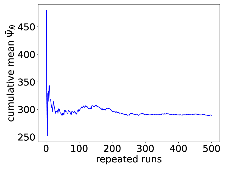
(a) Cumulative mean $\bar{\Psi}_{\tilde{N}}$ in (10)

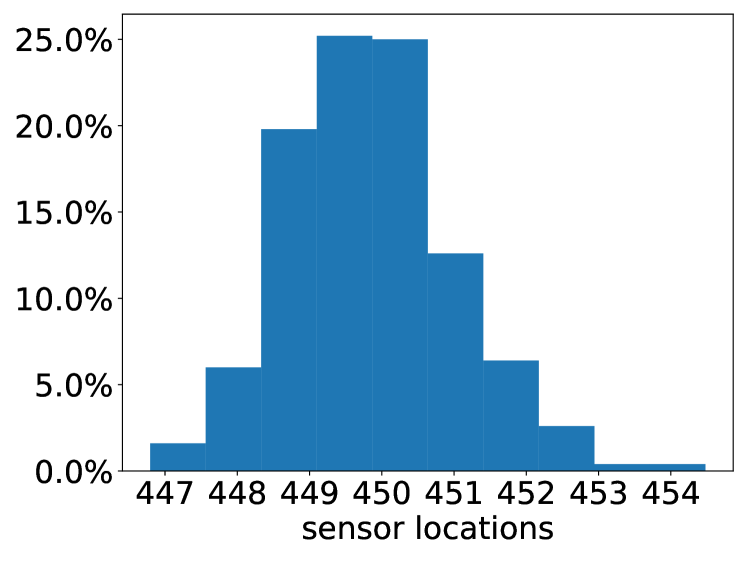
(b) Histogram of sensor locations

(c) Re-evaluated objective function, using a large $N=10,000$

Figure 3: Output of Example I(a)

For illustrative purposes, Example I considers the sensor placement along the horizontal line as shown in Figure 2. We start with placing 1 sensor in Example I(a). Let $\lambda_{1}=\lambda_{2}=0.0001$ for the inverse model (7), Figure 3 shows the results obtained from the rSAA algorithm. Figure 3(a) shows how the cumulative mean of the objective function changes against repeated runs (we set $\tilde{N}=5$), which appears to converge after $K=250$ runs. Figure 3(b) shows the histogram of optimal sensor locations from each run, and the mean of sensor location is found to be 449.8. Because we only consider the deployment of one sensor along a straight line, it is possible to re-evaluate the objective function (for validation purposes), using a large $N=10,000$, based on the optimal sensor locations from repeated runs; see Figure 3(c). The lowest point of this curve corresponds to the true optimal solution (i.e., 450.57 in Figure 3(c)). We see that, the solutions obtained from multiple repeated runs vary around the true optimal solution, and the average sensor location is close to the true optimal solution, justifying the necessity of repeating SAA runs. Figure 4 shows the (log) gap, defined in (10), against repeated runs, and the convergence of the algorithm is observed.

Figure 4: The stochastic upper bound defined in (10), $\alpha=0.025$.

(a) $\lambda_{1}=\lambda_{2}=0.01$, $J=30,000$

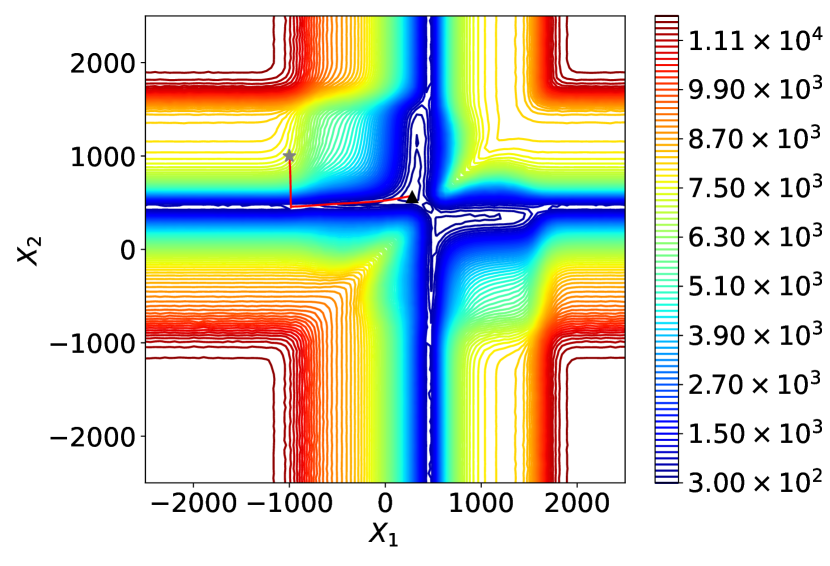
(b) $\lambda_{1}=\lambda_{2}=0.001$, $J=30,000$

(c) $\lambda_{1}=\lambda_{2}=0.01$, $J=30,000$

(d) $\lambda_{1}=\lambda_{2}=0.001$, $J=30,000$

Figure 5: Example I(b): trajectories for different initial guesses, $\lambda_{1}$ and $\lambda_{2}$ ($J=30,000$).

(a) $\lambda_{1}=\lambda_{2}=0.01$, $J=1$

(b) $\lambda_{1}=\lambda_{2}=0.001$, $J=1$

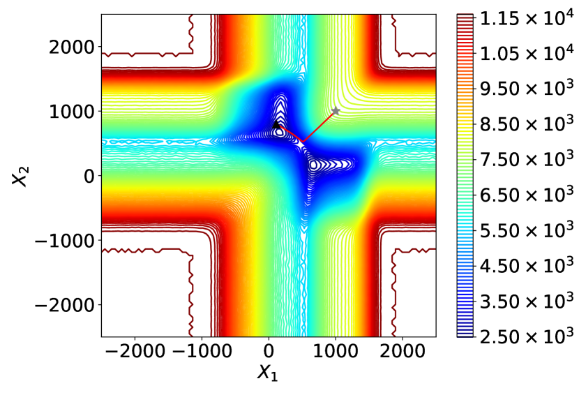
(c) $\lambda_{1}=\lambda_{2}=0.01$, $J=1$

(d) $\lambda_{1}=\lambda_{2}=0.001$, $J=1$

Figure 6: Example I(b): trajectories for different initial guesses, $\lambda_{1}$ and $\lambda_{2}$ ($J=1$).

In Example I(b), we consider the placement of 2 sensors along the same line using the SBA algorithm. Figure 5 shows the trajectories of the locations of these two sensors on the straight line given different initial guesses (marked by stars). The contour in this figure is the objective function $\hat{\Psi}_{N}(\bm{s})$ evaluated using a large number of Monte Carlo samples for different sensor locations. It is seen that the sensor location goes downhill as the iteration proceeds, which demonstrates the effectiveness of the algorithm. We also investigate if a small $J$ can be used in Algorithm 2, such as $J=1$, to further accelerate the inner solver. Because a smaller $J$ requires a larger $M$ for the algorithm to converge, we also double the value the $M$ when $J=1$. The result is shown in Figure 6 with different choices of $\lambda_{1}$ and $\lambda_{2}$. It is seen that the SBA algorithm still works well even when $J=1$. A drawback of a small $J=1$ is that there exists an inevitable gap between the best-found solution and the true minimum (of the contour), as shown in Figure 6(a) and 6(c) when $\lambda_{1}=\lambda_{2}=0.01$. The optimal selection of $\lambda$ in inverse modeling can also be formulated as a bilevel optimization problem; see reference [4]. Finally, the optimal locations of the 2 sensors are shown in Figure 2.

4.2 Example II: Sensor Placement over a Continuous 2D domain

In Example II, a more complex problem is considered for which sensors are placed over a continuous 2D domain with 10, 20, 50 and 100 emission sources. In this example, data are still generated from a Gaussian plume model.

We start with 10 emission sources, $\left\{\bm{x}_{j}\right\}_{j=1...10}$, distributed over a 2D domain, $[-25,25]\times[-25,25]$. We set the source locations $\left\{\bm{x}_{j}\right\}_{j=1...10}$ to $\{(-15,17)$, $(-10,-5)$, $(-9,22)$, $(-5,10)$, $(5,18)$, $(5,0)$, $(8,-10)$, $(10,19)$, $(15,-10)$, $(20,5)\}$. We assume that the emission strengths $\bm{\theta}=(\theta_{1},...,\theta_{10})$ follow a multivariate truncated (i.e., nonnegative) normal distribution obtained from a multivariate normal distribution $\mathcal{N}(\bm{\mu}_{\text{pr}},\bm{\Gamma}_{\text{pr}})$; see Proposition 3.1. Here, $\bm{\mu}_{\text{pr}}=(8,10,9,8,10,9,8,10,9,10)^{T}$, $\bm{\Gamma}_{\text{pr}}$ is a diagonal matrix, $\sigma^{2}_{Pr}\bm{I}$ where $\sigma_{Pr}=20$. The standard deviation of the observation noise is set to $0.01$. The distribution of wind vector is shown in Figure 7, where the wind speed is uniformly sampled between $[1,2]$, and the wind direction is sampled between north-west and north-east. The SBA algorithm is used to find the optimal sensor locations. For the inner problem, we let $\lambda_{1}=\lambda_{2}=0.01$, and $J=2000$. The learning rate $\tau_{m,j}=0.0005$ for any $m$ and $j$. For the outer loop, the learning rate $\rho_{m}=0.00005$ for any $m$. The re-sampling size $\tilde{N}$ is set to 100.

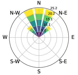
Figure 7: Wind rose plot

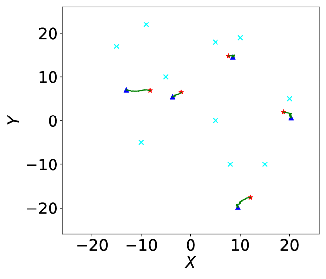
(a) updates of sensor locations ($M$=300)

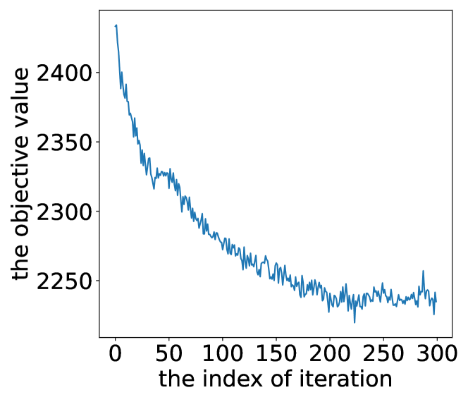
(b) objective value along iterations

Figure 8: Deployment of 5 sensors for 10 emission sources.

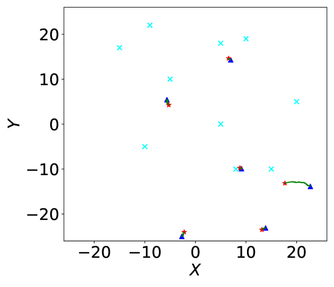
(a) updates of sensor locations ($M$=300)

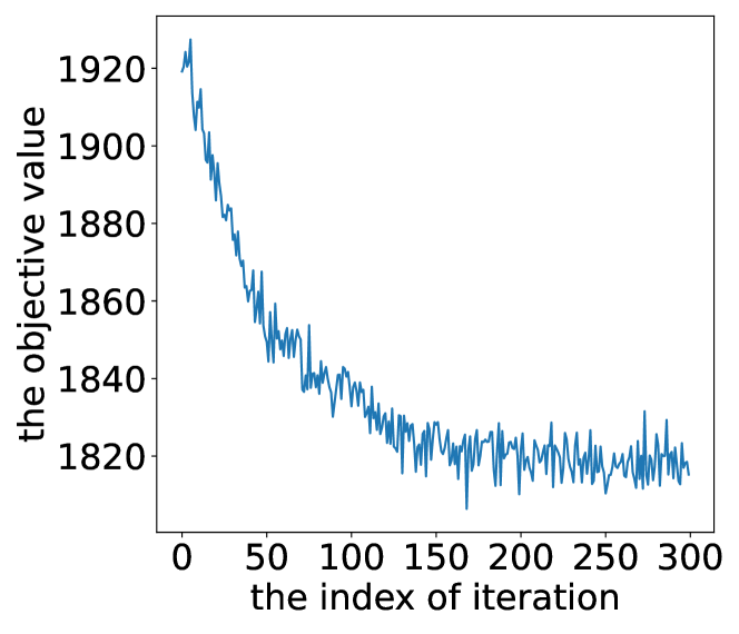
(b) objective value along iterations

Figure 9: Deployment of 6 sensors for 10 emission sources.

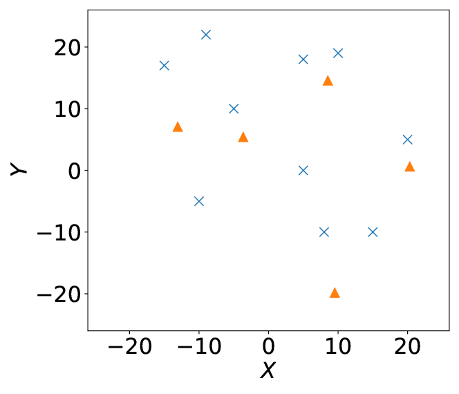
(a) 5 sensors

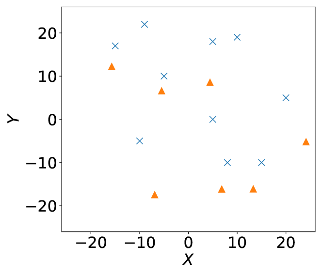
(b) 7 sensors

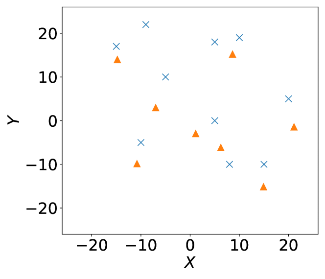
(c) 8 sensors

(d) 9 sensors

Figure 10: Final deployment of 5, 7, 8 and 9 sensors for 10 emission sources.

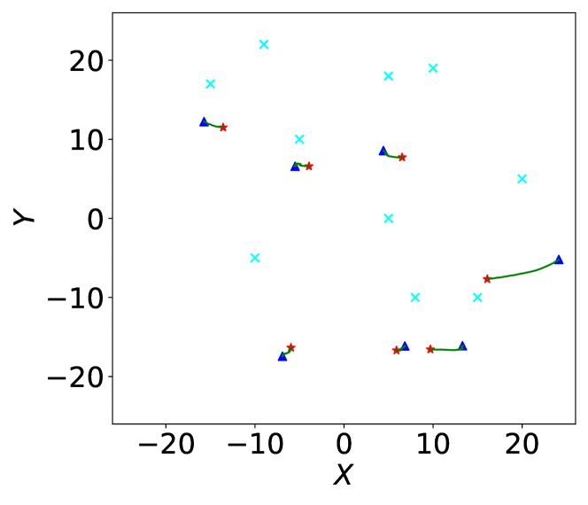
(a) updates of sensor locations ($M$=300)

(b) objective value along iterations

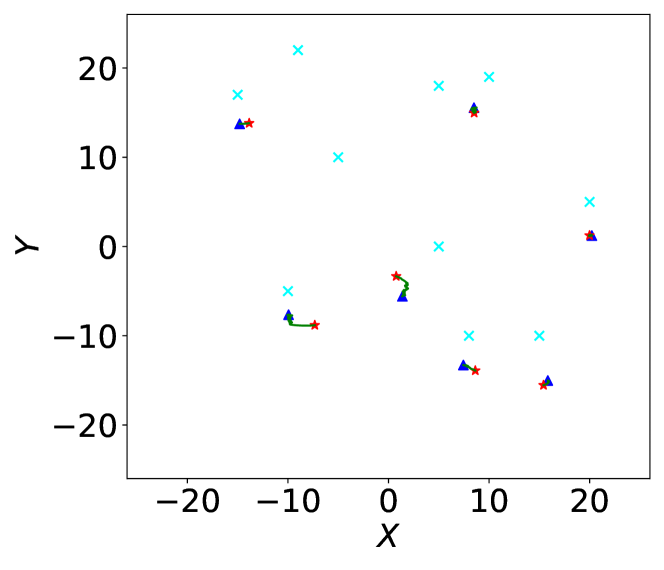
(c) updates of sensor locations ($M$=300)

(d) objective value along iterations

Figure 11: Allocation of 7 sensors for 10 emission sources with different initial guesses

The locations of sensors and the corresponding objective values along the iterations are shown Figures 8 and 9. In these figures, the objective value is re-evaluated with large Monte Carlo samples (i.e., 100,000 samples) for each iteration step, and the iteration number $M$ for the outer problem is chosen according to the computing budget. We see that the SBA algorithm is able to iteratively optimize sensor allocation with decreasing objective values in most cases. In Appendix 6.4, we present more results on different scenarios of the number of sensors, number of emission sources, initial sensor locations, and inner problem iteration limit $J$. Figure 10 shows the final allocation of 5, 7, 8 and 9 sensors for 10 emission sources.

It is also worth noting that the final sensor locations highly depend on the initial guess. In Figure 11(a) and 11(c), we generate different initial sensor locations, and obtain different final designs. In other words, the solutions reach different local optimums (or saddle points) due to different initial sensor locations, and the objective value also converges differently to the corresponding local minimum, as shown in Figure 11(b) and 11(d). We also note that the proposed approximate $A$-optimal design provides a better initial guess than random guesses.

We also investigated the effect of the inner iteration number $J$ on the final designs of sensor locations. A small $J$ affects the choice of the outer learning rate $\rho_{m}$ and outer iteration number $M$. Based on our numerical experiments, a small $J$ reduces the total computational time but may cause oscillation along iterations if the same outer learning rate is used. For example, we compare $J=2000$ and $J=200$ for the 7-sensor placement task, as shown by Figure 11(a) and 21(a) (in the Appendix). Both settings converge to local optimums but a ‘ziggy’ movement of sensor locations is observed when $J=200$. Considering their similar final objective value, as shown by Figure 11(b) and 21(b) (in the Appendix), a small $J$ appears to be good enough to find a local optimum. Of course, the ‘ziggy’ movement, due to a small $J$, could make the solution diverge from the current valley. To avoid the ‘ziggy’ pattern of small $J$, a small outer learning rate $\rho_{m}$ is needed. Again, this affects the convergence rate: a large $J=2000$ leads to a smaller inner optimality gap, but the computation of the hypergradient becomes more expensive. Since a smaller inner optimality gap makes the upper bound tighter (as shown in Theorems 3.3 and 3.4), there is a trade-off between the upper bound assurance and the computational time affected by $J$.

To illustrate the trade-off above, Figure 12 shows the designs for 20 emission sources whose locations are randomly selected. We compare $\rho_{m}=5\times 10^{-7}$ and $\rho_{m}=1\times 10^{-6}$ for $J=1$. In this case, $\rho_{m}=5\times 10^{-7}$ and $\rho_{m}=1\times 10^{-6}$ lead to similar final designs with the same iteration numbers, so $\rho_{m}=1\times 10^{-6}$ is better in this case.

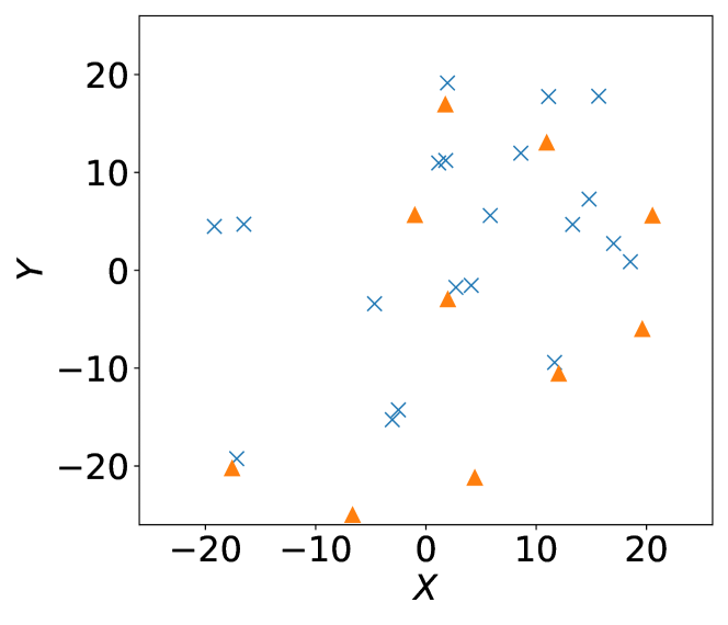
(a) $J=1$, $\rho_{m}=5\times 10^{-7}$ and $M=3000$

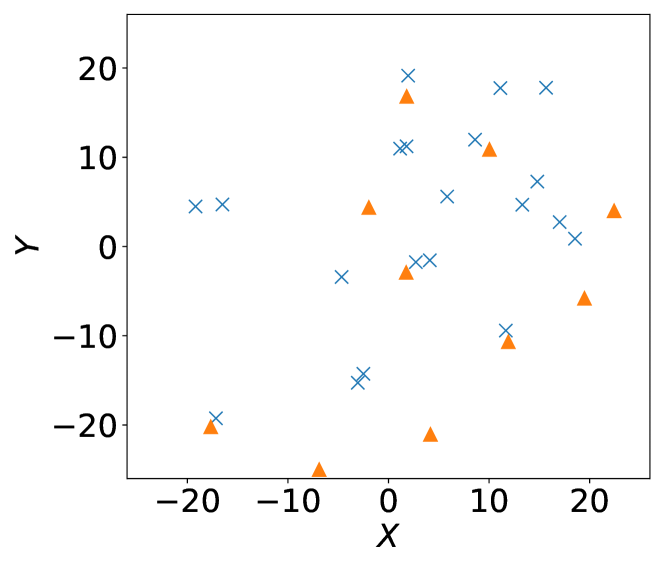
(b) $J=1$, $\rho_{m}=1\times 10^{-6}$ and $M=3000$

Figure 12: Allocation of 10 sensors for 20 emission sources.

Finally, we place multiple sensors, 10, 20, and 30, for 50 emission sources and place 50 sensors for 100 emission sources. When 10 sensors are deployed for 50 sources, Figure 13 shows that 4 out of 10 sensors are finally placed on the bottom boundary because of the north-to-south wind direction. The deployment of 20 and 30 sensors are shown in Figure 14, and the deployment of 50 sensors is shown in Figure 15. For all of these scenarios, there are always sensors evenly placed on the bottom boundary.

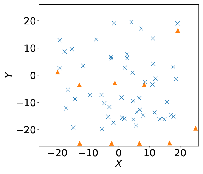
(a) $J=1$, $\rho_{m}=5\times 10^{-7}$ and $M=3000$

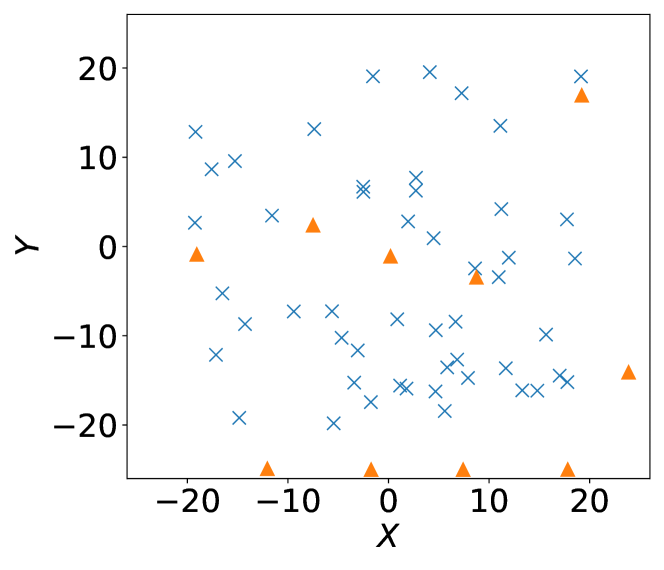
(b) $J=1$, $\rho_{m}=1\times 10^{-6}$ and $M=300$

Figure 13: Allocation of 10 sensors for 50 sources.

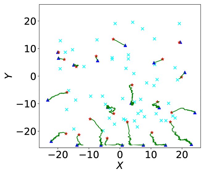
(a) 20 sensors, $M$=500

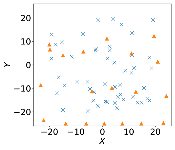
(b) 20 sensors, $M$=500

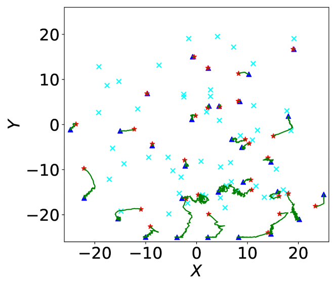
(c) 30 sensors, $M$=300

(d) 30 sensors, $M$=300

Figure 14: Sensor placement for 50 emission sources.

(a) trajectory

(b) Final locations of sensors

Figure 15: Placement of 50 sensors for 100 emission sources ($M=1000$).

4.3 Validation

In this subsection, we further validate the performance of emission estimation based on the sensor allocation obtained above. In particular, we focus on the placement of 10 sensors for 20 sources in subsection 4.2 (see Figure 16), and compare different designs, emission uncertainties, and observational noise. The wind profile is still defined as Figure 7.

Figure 17 shows the effect of observation noise and emission uncertainty (i.e., $\sigma_{Pr}$) on estimation error. It is seen that a larger observation noise increases the estimation error. Figure 18 shows both the estimated and true emission rates for different emission sources. It is seen that source E15 (at the bottom left corner) is not well covered by the sensor network, and this explains a less accurate estimated emission rate for E15. In Figure 18, we compare the random design (i.e., randomly placed sensors), the initial design based on Proposition 3.1, and our design under the same settings. It is seen that the boxplots of actual emission rates are closer to that of the estimated rates based on our design. The MAPE (Mean Absolute Percentage Error) are respectively $69.06\%$, $50.79\%$ and $29.94\%$ for the random design, the initial design based on Proposition 3.1, and the optimal design obtained.

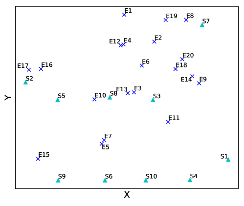
Figure 16: Allocation of 10 sensors (S1-S10) for 20 sources (E1-E20)

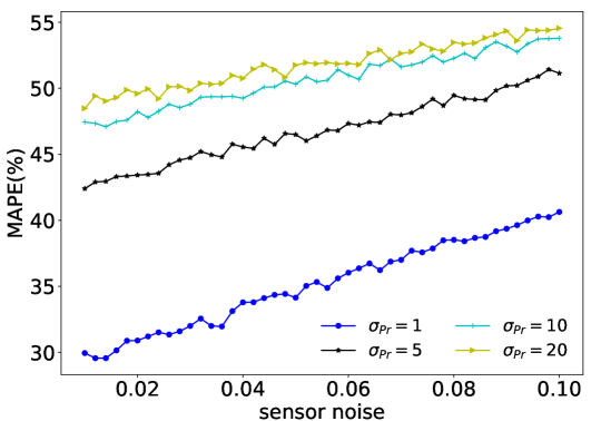
Figure 17: Effect of sensor noise and emission uncertainty on estimation error.

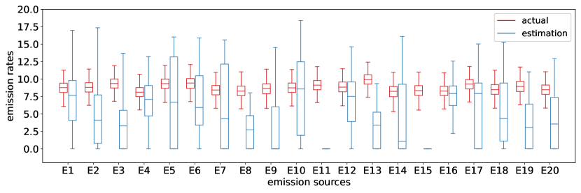
(a) Random design

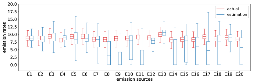
(b) The initial design based on Proposition 3.1

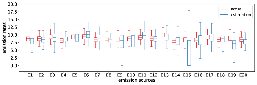
(c) The proposed design in Figure 16

Figure 18: Comparison of the estimated emission rates based on different sensor allocations

5 Conclusions

This paper investigated the optimal sensor placement problem using bilevel optimization. The paper considered linear inverse models when the closed-form designs do not exist due to the non-negativity constraints on the inversion estimates. Two algorithms, including rSAA and SBA, have been utilized, and their performance guarantees have also been obtained by convergence analysis. Comprehensive numerical investigations demonstrated the effectiveness of the proposed approach. Note that, this paper only considers the sensor deployment in a 2D domain. A challenging extension is to consider the sensor allocation problems in the 3D space, including the height, which require incorporating surface terrain modeling and computationally efficient algorithms.

6 Appendix

6.1 Appendix I

Proof of Proposition 3.1:
Consider an observation model as follows,

(31) $$\bm{\Phi}(\bm{\beta},\bm{s})=\mathcal{F}(\bm{\beta},\bm{s})\bm{\theta}+\bm{\epsilon},\ \bm{\epsilon}\sim\mathcal{N}(\bm{0},\bm{\Gamma}_{\bm{\epsilon}}(\bm{s}))$$

where $\bm{\epsilon}$ is the additive Gaussian noise, and $\mathcal{F}:\mathbb{R}^{N_{p}}\mapsto\mathbb{R}^{d}$ is a linear parameter-to-observation mapping. Let $\bm{\theta}\sim\mathcal{N}(\bm{\mu}_{\text{pr}},\bm{\Gamma}_{\text{pr}})$ be the prior distribution of $\bm{\theta}$, we obtain the posterior distribution $\bm{\theta}_{\text{post}}(\bm{\beta},\bm{s})\sim\mathcal{N}(\bm{\mu}_{\text{post}}(\bm{\beta},\bm{s}),\bm{\Gamma}_{\text{post}}(\bm{\beta},\bm{s}))$, and

(32) $$\begin{split}\bm{\mu}_{\text{post}}(\bm{\beta},\bm{s})&=\bm{\Gamma}_{\text{post}}(\mathcal{F}^{*}(\bm{\beta},\bm{s})\bm{\Gamma}^{-1}_{\bm{\epsilon}}(\bm{s})\bm{\Phi}(\bm{\beta},\bm{s})+\bm{\Gamma}^{-1}_{\text{pr}}\bm{\mu}_{\text{pr}})\\ \bm{\Gamma}_{\text{post}}(\bm{\beta},\bm{s})&=(\mathcal{F}^{*}(\bm{\beta},\bm{s})\bm{\Gamma}^{-1}_{\bm{\epsilon}}(\bm{s})\mathcal{F}(\bm{\beta},\bm{s})+\bm{\Gamma}^{-1}_{pr})^{-1}\end{split}$$

where $F^{*}(\bm{\beta},\bm{s})$ is the adjoint of $F$, e.g., by solving the adjoint PDE model. It is noted that $F^{*}(\bm{\beta},\bm{s})=F^{T}(\bm{\beta},\bm{s})$ because of its linear operator property.

Then, the Bayesian risk is defined as,

(33) $$\begin{split}\Psi_{\text{risk, linear, Gaussian}}(\bm{s})&=\mathbb{E}_{\bm{\theta},\bm{\beta}}\Bigg{\{}\mathbb{E}_{\bm{\Phi}|\bm{\theta},\bm{\beta}}\Big{\{}\Big{\|}\hat{\bm{\theta}}_{MAP}(\bm{\Phi},\bm{\beta},\bm{s})-\bm{\theta}\Big{\|}^{2}_{2}\Big{\}}\Bigg{\}}\\ &=\mathbb{E}_{\bm{\beta}}\Bigg{\{}\mathbb{E}_{\bm{\theta}|\bm{\beta}}\Bigg{\{}\mathbb{E}_{\bm{\Phi}|\bm{\theta},\bm{\beta}}\Big{\{}\Big{\|}\hat{\bm{\theta}}_{MAP}(\bm{\Phi},\bm{\beta},\bm{s})-\bm{\theta}\Big{\|}^{2}_{2}\Big{\}}\Bigg{\}}\Bigg{\}}\end{split}$$

For convenience, we respectively denote $\mathcal{F}(\bm{\beta},\bm{s})$, $\mathcal{F}^{*}(\bm{\beta},\bm{s})$, $\bm{\Phi}(\bm{\beta},\bm{s})$, $\bm{\Gamma}_{\text{post}}(\bm{\beta},\bm{s})$ and $\bm{\Gamma}^{-1}_{\bm{\epsilon}}(\bm{s})$ by $\mathcal{F}$, $\mathcal{F}^{*}$, $\bm{\Phi}$, $\bm{\Gamma}_{\text{post}}$, and $\bm{\Gamma}^{-1}_{\bm{\epsilon}}$. Then, we expand the $L^{2}$ loss function as

(34) $$\begin{split}\Big{\|}\hat{\bm{\theta}}_{MAP}(\bm{\Phi},\bm{\beta},\bm{s})-\bm{\theta}\Big{\|}^{2}_{2}=\Big{\|}(\bm{\Gamma}_{\text{post}}\mathcal{F}^{*}\bm{\Gamma}^{-1}_{\bm{\epsilon}}\mathcal{F}-\bm{I})\bm{\theta}+\bm{\Gamma}_{\text{post}}(\mathcal{F}^{*}\bm{\Gamma}^{-1}_{\bm{\epsilon}}\bm{\epsilon}+\bm{L}^{T}\bm{L}\bm{\mu}_{\text{pr}})\Big{\|}^{2}_{2}\end{split}$$

where $\bm{L}^{T}\bm{L}=\bm{\Gamma}^{-1}_{pr}$.

Denote $\bm{M}(\bm{s})=\bm{\Gamma}_{\text{post}}\mathcal{F}^{*}\bm{\Gamma}^{-1}_{\bm{\epsilon}}\mathcal{F}-\bm{I}$, we can further obtain

(35) $$\begin{split}\Big{\|}\hat{\bm{\theta}}_{MAP}(\bm{\Phi},\bm{\beta},\bm{s})-\bm{\theta}\Big{\|}^{2}_{2}=\Big{\|}\bm{M}(\bm{s})\bm{\theta}+\bm{\Gamma}_{\text{post}}(\mathcal{F}^{*}\bm{\Gamma}^{-1}_{\bm{\epsilon}}\bm{\epsilon}+\bm{L}^{T}\bm{L}\bm{\mu}_{\text{pr}})\Big{\|}^{2}_{2}\end{split}$$

Then, plugging (35) into the expectation over $\bm{\theta}|\bm{\beta}$ yields

(36) $$\begin{split}&\ \ \ \mathbb{E}_{\bm{\theta}|\bm{\beta}}\Bigg{\{}\mathbb{E}_{\bm{\Phi}|\bm{\theta},\bm{\beta}}\Big{\{}\Big{\|}\hat{\bm{\theta}}_{MAP}(\bm{\Phi},\bm{\beta},\bm{s})-\bm{\theta}\Big{\|}^{2}_{2}\Big{\}}\Bigg{\}}\\ &=\mathbb{E}_{\bm{\theta}|\bm{\beta}}\Bigg{\{}\mathbb{E}_{\bm{\Phi}|\bm{\theta},\bm{\beta}}\Big{\{}\bm{\theta}^{T}\bm{M}^{T}(\bm{s})\bm{M}(\bm{s})\bm{\theta}\Big{\}}\Bigg{\}}+\mathbb{E}_{\bm{\theta}|\bm{\beta}}\Bigg{\{}\mathbb{E}_{\bm{\Phi}|\bm{\theta},\bm{\beta}}\Big{\{}2\bm{\theta}^{T}\bm{M}^{T}(\bm{s})\bm{\Gamma}_{\text{post}}(\mathcal{F}^{*}\bm{\Gamma}^{-1}_{\bm{\epsilon}}\bm{\epsilon}+\bm{L}^{T}\bm{L}\bm{\mu}_{\text{pr}})\Big{\}}\Bigg{\}}\\ &\ \ \ +\mathbb{E}_{\bm{\theta}|\bm{\beta}}\Bigg{\{}\mathbb{E}_{\bm{\Phi}|\bm{\theta},\bm{\beta}}\Big{\{}(\mathcal{F}^{*}\bm{\Gamma}^{-1}_{\bm{\epsilon}}\bm{\epsilon}+\bm{L}^{T}\bm{L}\bm{\mu}_{\text{pr}})^{T}\bm{\Gamma}^{T}_{\text{post}}\bm{\Gamma}_{\text{post}}(\mathcal{F}^{*}\bm{\Gamma}^{-1}_{\bm{\epsilon}}\bm{\epsilon}+\bm{L}^{T}\bm{L}\bm{\mu}_{\text{pr}})\Big{\}}\Bigg{\}}\end{split}$$

Recall that $\bm{\epsilon}\sim\mathcal{N}(\bm{0},\bm{\Gamma}_{\bm{\epsilon}}(\bm{s}))$, $\bm{\theta}\sim\mathcal{N}(\bm{\mu}_{\text{pr}},\bm{\Gamma}_{\text{pr}})$, and $\bm{\theta}\sim\mathcal{N}(\bm{\mu}_{\text{pr}},\bm{\Gamma}_{\text{pr}})$, we obtain

(37) $$\begin{split}&\ \ \ \mathbb{E}_{\bm{\theta}|\bm{\beta}}\Bigg{\{}\mathbb{E}_{\bm{\Phi}|\bm{\theta},\bm{\beta}}\Big{\{}\Big{\|}\hat{\bm{\theta}}_{MAP}(\bm{\Phi},\bm{\beta},\bm{s})-\bm{\theta}\Big{\|}^{2}_{2}\Big{\}}\Bigg{\}}\\ &=\mathbb{E}_{\bm{\theta}|\bm{\beta}}\Bigg{\{}\mathbb{E}_{\bm{\Phi}|\bm{\theta},\bm{\beta}}\Big{\{}\bm{\theta}^{T}\bm{M}^{T}(\bm{s})\bm{M}(\bm{s})\bm{\theta}\Big{\}}\Bigg{\}}+2\bm{\mu}_{\text{pr}}^{T}\bm{M}^{T}(\bm{s})\bm{\Gamma}_{\text{post}}\bm{L}^{T}\bm{L}\bm{\mu}_{\text{pr}}\\ &\ \ \ +\mathbb{E}_{\bm{\theta}|\bm{\beta}}\Bigg{\{}\mathbb{E}_{\bm{\Phi}|\bm{\theta},\bm{\beta}}\Big{\{}\bm{\epsilon}^{T}\bm{\Gamma}^{-T}_{\bm{\epsilon}}\mathcal{F}\bm{\Gamma}^{T}_{\text{post}}\bm{\Gamma}_{\text{post}}\mathcal{F}^{*}\bm{\Gamma}^{-1}_{\bm{\epsilon}}\bm{\epsilon}\Big{\}}\Bigg{\}}\bm{\mu}^{T}_{\text{pr}}\bm{L}^{T}\bm{L}\bm{\Gamma}^{T}_{\text{post}}\bm{\Gamma}_{\text{post}}\bm{L}^{T}\bm{L}\bm{\mu}_{\text{pr}}.\end{split}$$

Because $\mathbb{E}(\bm{\delta}^{T}\bm{\Lambda}\bm{\delta})=\bm{\mu}^{T}_{\bm{\delta}}\bm{\Lambda}\bm{\mu}_{\bm{\delta}}+\text{tr}(\bm{\Lambda}\bm{\Gamma}_{\bm{\delta}})$, where $\bm{\delta}\sim\mathcal{N}(\bm{\mu}_{\bm{\delta}},\bm{\Gamma}_{\bm{\delta}})$, it follows from (37) that

(38) $$\begin{split}&\ \ \ \mathbb{E}_{\bm{\theta}|\bm{\beta}}\Bigg{\{}\mathbb{E}_{\bm{\Phi}|\bm{\theta},\bm{\beta}}\Big{\{}\Big{\|}\hat{\bm{\theta}}_{MAP}(\bm{\Phi},\bm{\beta},\bm{s})-\bm{\theta}\Big{\|}^{2}_{2}\Big{\}}\Bigg{\}}\\ &=\bm{\mu}^{T}_{\text{pr}}\bm{M}^{T}(\bm{s})\bm{M}(\bm{s})\bm{\mu}_{\text{pr}}+\text{tr}(\bm{M}^{T}(\bm{s})\bm{M}(\bm{s})\bm{\Gamma}_{\text{pr}})+2\bm{\mu}_{\text{pr}}^{T}\bm{M}^{T}(\bm{s})\bm{\Gamma}_{\text{post}}\bm{L}^{T}\bm{L}\bm{\mu}_{\text{pr}}+\text{tr}(\bm{\Gamma}^{-T}_{\bm{\epsilon}}\mathcal{F}\bm{\Gamma}^{T}_{\text{post}}\bm{\Gamma}_{\text{post}}\mathcal{F}^{*})\\ &\ \ \ +\bm{\mu}^{T}_{\text{pr}}\bm{L}^{T}\bm{L}\bm{\Gamma}^{T}_{\text{post}}\bm{\Gamma}_{\text{post}}\bm{L}^{T}\bm{L}\bm{\mu}_{\text{pr}}\end{split}$$

where the first, third and fifth terms on the right hand side can be written as $\|\bm{M}(\bm{s})\bm{\mu}_{\text{pr}}+\bm{\Gamma}_{\text{post}}\bm{L}^{T}\bm{L}\bm{\mu}_{\text{pr}}\|^{2}_{2}$, which turns out to be zero as follows

(39) $$\begin{split}&\|\bm{M}(\bm{s})\bm{\mu}_{\text{pr}}+\bm{\Gamma}_{\text{post}}\bm{L}^{T}\bm{L}\bm{\mu}_{\text{pr}}\|^{2}_{2}\\ &=\|(\bm{M}(\bm{s})+\bm{\Gamma}_{\text{post}}\bm{L}^{T}\bm{L})\bm{\mu}_{\text{pr}}\|^{2}_{2}\\ &=\|(\bm{\Gamma}_{\text{post}}\mathcal{F}^{*}\bm{\Gamma}^{-1}_{\bm{\epsilon}}\mathcal{F}-\bm{I}+\bm{\Gamma}_{\text{post}}\bm{L}^{T}\bm{L})\bm{\mu}_{\text{pr}}\|^{2}_{2}\\ &=\|(\bm{\Gamma}_{\text{post}}(\mathcal{F}^{*}\bm{\Gamma}^{-1}_{\bm{\epsilon}}\mathcal{F}+\bm{L}^{T}\bm{L})-\bm{I})\bm{\mu}_{\text{pr}}\|^{2}_{2}\\ &=\bm{0}\end{split}$$

Then we can rewrite (38) as

(40) $$\begin{split}\mathbb{E}_{\bm{\theta}|\bm{\beta}}\Bigg{\{}\mathbb{E}_{\bm{\Phi}|\bm{\theta},\bm{\beta}}\Big{\{}\Big{\|}\hat{\bm{\theta}}_{MAP}(\bm{\Phi},\bm{\beta},\bm{s})-\bm{\theta}\Big{\|}^{2}_{2}\Big{\}}\Bigg{\}}=\text{tr}(\bm{M}^{T}(\bm{s})\bm{M}(\bm{s})\bm{\Gamma}_{\text{pr}})+\text{tr}(\bm{\Gamma}^{-T}_{\bm{\epsilon}}\mathcal{F}\bm{\Gamma}^{T}_{\text{post}}\bm{\Gamma}_{\text{post}}\mathcal{F}^{*})\end{split}$$

where the first term on the right hand side can be further transformed according to $\bm{M}(\bm{s})\bm{L}^{-1}=-\bm{\Gamma}_{\text{post}}\bm{L}^{T}$ given by (39),

(41) $$\begin{split}\text{tr}(\bm{M}^{T}(\bm{s})\bm{M}(\bm{s})\bm{\Gamma}_{\text{pr}})=\Big{\|}\bm{\Gamma}_{\text{post}}\bm{L}^{T}\Big{\|}^{2}_{F}\end{split}$$

For the second term on the right hand side of (40), we further transform it by defining $\bm{\Gamma}^{-1}_{\bm{\epsilon}}=\bm{U}^{T}\bm{U}$ as follows

(42) $$\begin{split}\text{tr}(\bm{\Gamma}^{-T}_{\bm{\epsilon}}\mathcal{F}\bm{\Gamma}^{T}_{\text{post}}\bm{\Gamma}_{\text{post}}\mathcal{F}^{*})=\Big{\|}\bm{\Gamma}_{\text{post}}\mathcal{F}^{*}\bm{U}^{T}\Big{\|}^{2}_{F}\end{split}$$

After plugging (41)(42) into (40), we achieve

(43) $$\begin{split}\mathbb{E}_{\bm{\theta}|\bm{\beta}}\Bigg{\{}\mathbb{E}_{\bm{\Phi}|\bm{\theta},\bm{\beta}}\Big{\{}\Big{\|}\hat{\bm{\theta}}_{MAP}(\bm{\Phi},\bm{\beta},\bm{s})-\bm{\theta}\Big{\|}^{2}_{2}\Big{\}}\Bigg{\}}=\Big{\|}\bm{\Gamma}_{\text{post}}\bm{L}^{T}\Big{\|}^{2}_{F}+\Big{\|}\bm{\Gamma}_{\text{post}}\mathcal{F}^{*}\bm{U}^{T}\Big{\|}^{2}_{F}\end{split}$$

Finally, we plug (43) into (33) to obtain the closed-form optimization objective

(44) $$\begin{split}\hat{\Psi}_{\text{risk, linear, Gaussian}}(\bm{s})=\mathbb{E}_{\bm{\beta}}\Bigg{\{}\Big{\|}\bm{\Gamma}_{\text{post}}\bm{L}^{T}\Big{\|}^{2}_{F}+\Big{\|}\bm{\Gamma}_{\text{post}}\mathcal{F}^{*}\bm{U}^{T}\Big{\|}^{2}_{F}\Bigg{\}}\end{split}.$$

6.2 Appendix II

To compute $\nabla_{\bm{s}}\big{(}\bm{C}(\bm{\beta}^{(i)},\bm{s})\bm{\theta}^{(i)}+\bm{d}^{T}(\bm{\beta}^{(i)},\bm{\Phi}^{(i)},\bm{s})\big{)}$, we need the gradients

(45) $$\frac{\partial A_{m}A_{n}}{\partial s_{i,1}},\ \frac{\partial A_{m}A_{n}}{\partial s_{i,2}},\ \frac{\partial A_{m}}{\partial s_{i,1}},\ \frac{\partial A_{m}}{\partial s_{i,2}}$$

Below are the derivations of these gradients:

Given the Gaussian plume kernel [43]

(46) $$A_{j}(\bm{s}_{i})=\frac{1}{2\pi K\|(\bm{s}_{i}-\bm{x}_{j})\cdot\bm{\beta}^{\parallel}\|}\text{exp}\Big{(}-\frac{u\big{(}\|(\bm{s}_{i}-\bm{x}_{j})\cdot\bm{\beta}^{\perp}\|^{2}+H^{2}\big{)}}{4K\|(\bm{s}_{i}-\bm{x}_{j})\cdot\bm{\beta}^{\parallel}\|}\Big{)},$$

let $\bm{r}_{\parallel}^{(j)}=(\bm{s}_{i}-\bm{x}_{j})\cdot\bm{\beta}^{\parallel}$ and $\bm{r}_{\perp}^{(j)}=(\bm{s}_{i}-\bm{x}_{j})\cdot\bm{\beta}^{\perp}$ for simplicity, we denote

(47) $$A_{j}=\frac{1}{2\pi K|\bm{r}_{\parallel}^{(j)}|}\text{exp}\Big{(}-\frac{u\big{(}|\bm{r}_{\perp}^{(j)}|^{2}+H^{2}\big{)}}{4K|\bm{r}_{\parallel}^{(j)}|}\Big{)}.$$

Then, we can get

(48) $$A_{m}A_{n}=\frac{1}{4\pi^{2}K^{2}|\bm{r}_{\parallel}^{(m)}|\cdot|\bm{r}_{\parallel}^{(n)}|}\text{exp}\Big{(}\frac{-u\big{(}|\bm{r}_{\perp}^{(m)}|^{2}+H^{2}\big{)}}{4K|\bm{r}_{\parallel}^{(m)}|}+\frac{-u\big{(}|\bm{r}_{\perp}^{(n)}|^{2}+H^{2}\big{)}}{4K|\bm{r}_{\parallel}^{(n)}|}\Big{)}.$$

By denoting $\bm{w}=(w_{1},w_{2})=\frac{\bm{\beta}}{|\bm{\beta}|}$, $\bm{s}_{i}=(s_{i,1},s_{i,2})$, $\bm{x}_{j}=(x_{j,1},x_{j,2})$, and $\bm{r}^{(j)}=(s_{i,1}-x_{j,1},s_{i,2}-x_{j,2})$, we can derive $\bm{r}_{\parallel}^{(j)}$, $|\bm{r}_{\parallel}^{(j)}|$, $\bm{r}_{\perp}^{(j)}$, $|\bm{r}_{\perp}^{(j)}|$ as,

$$\begin{split}&\bm{r}_{\parallel}^{(j)}=(w_{1}(s_{i,1}-x_{j,1})+w_{2}(s_{i,2}-x_{j,2}))\cdot(w_{1},w_{2})\\ &|\bm{r}_{\parallel}^{(j)}|=w_{1}(s_{i,1}-x_{j,1})+w_{2}(s_{i,2}-x_{j,2})\\ &\bm{r}_{\perp}^{(j)}=\bm{r}^{(j)}-\bm{r}_{\parallel}^{(j)}\\ &=\Big{(}s_{i,1}-x_{j,1}-w_{1}[w_{1}(s_{i,1}-x_{j,1})+w_{2}(s_{i,2}-x_{j,2})],s_{i,2}-x_{j,2}-w_{2}[w_{1}(s_{i,1}-x_{j,1})+w_{2}(s_{i,2}-x_{j,2})]\Big{)}\\ &=\Big{(}(1-w_{1}^{2})(s_{i,1}-x_{j,1})-w_{1}w_{2}(s_{i,2}-x_{j,2}),-w_{1}w_{2}(s_{i,1}-x_{j,1})+(1-w_{2}^{2})(s_{i,2}-x_{j,2})\Big{)}\\ &|\bm{r}_{\perp}^{(j)}|=\sqrt{\Big{(}\big{[}(1-w_{1}^{2})(s_{i,1}-x_{j,1})-w_{1}w_{2}(s_{i,2}-x_{j,2})\big{]}^{2}+\big{[}-w_{1}w_{2}(s_{i,1}-x_{j,1})+(1-w_{2}^{2})(s_{i,2}-x_{j,2})\big{]}^{2}\Big{)}}\end{split}$$

Then we can derive the gradients of $A_{m}A_{n}$ w.r.t $s_{i,1}$ and $s_{i,2}$,

(49) $$\begin{split}\frac{\partial A_{m}A_{n}}{\partial s_{i,1}}=&\frac{-1}{\big{[}4\pi^{2}K^{2}|\bm{r}_{\parallel}^{(m)}|\cdot|\bm{r}_{\parallel}^{(n)}|\big{]}^{2}}4\pi^{2}K^{2}w_{1}\Big{[}|\bm{r}_{\parallel}^{m}|+|\bm{r}_{\parallel}^{n}|\Big{]}\cdot\text{exp}\Big{(}\frac{-u\big{(}|\bm{r}_{\perp}^{(m)}|^{2}+H^{2}\big{)}}{4K|\bm{r}_{\parallel}^{(m)}|}+\frac{-u\big{(}|\bm{r}_{\perp}^{(n)}|^{2}+H^{2}\big{)}}{4K|\bm{r}_{\parallel}^{(n)}|}\Big{)}+\\ &\frac{1}{4\pi^{2}K^{2}|\bm{r}_{\parallel}^{(m)}|\cdot|\bm{r}_{\parallel}^{(n)}|}\cdot\text{exp}\Big{(}\frac{-u\big{(}|\bm{r}_{\perp}^{(m)}|^{2}+H^{2}\big{)}}{4K|\bm{r}_{\parallel}^{(m)}|}+\frac{-u\big{(}|\bm{r}_{\perp}^{(n)}|^{2}+H^{2}\big{)}}{4K|\bm{r}_{\parallel}^{(n)}|}\Big{)}\cdot\Big{(}\frac{\partial\normalsize{\scriptsize{1}⃝}\normalsize}{\partial s_{i,1}}+\frac{\partial\normalsize{\scriptsize{2}⃝}\normalsize}{\partial s_{i,1}}\Big{)}\end{split}$$

and similarly, we can obtain the gradients of $A_{m}$ w.r.t $s_{i,1}$,

(50) $$\frac{\partial A_{m}}{\partial s_{i,1}}=\frac{-1\cdot 2\pi Kw_{1}}{(2\pi K|\bm{r}_{\parallel}^{(m)}|)^{2}}\text{exp}\Big{(}\frac{-u\big{(}|\bm{r}_{\perp}^{(m)}|^{2}+H^{2}\big{)}}{4K|\bm{r}_{\parallel}^{(m)}|}\Big{)}+\frac{1}{2\pi K|\bm{r}_{\parallel}^{(m)}|}\text{exp}\Big{(}\frac{-u\big{(}|\bm{r}_{\perp}^{(m)}|^{2}+H^{2}\big{)}}{4K|\bm{r}_{\parallel}^{(m)}|}\Big{)}\cdot\frac{\partial\normalsize{\scriptsize{1}⃝}\normalsize}{\partial s_{i,1}}$$

where

$$\begin{split}&\frac{\partial\normalsize{\scriptsize{1}⃝}\normalsize}{\partial s_{i,1}}=\frac{-u\Big{[}2\cdot\normalsize{\scriptsize{3}⃝}\normalsize\cdot(1-w_{1}^{2})+2\cdot\normalsize{\scriptsize{4}⃝}\normalsize\cdot(-w_{1}w_{2})\Big{]}4K|\bm{r}_{\parallel}^{(m)}|-\Big{(}-u\big{(}|\bm{r}_{\perp}^{(m)}|^{2}+H^{2}\big{)}4Kw_{1}\Big{)}}{(4K|\bm{r}_{\parallel}^{(m)}|)^{2}}\\ &\frac{\partial\normalsize{\scriptsize{2}⃝}\normalsize}{\partial s_{i,1}}=\frac{-u\Big{[}2\cdot\normalsize{\scriptsize{5}⃝}\normalsize\cdot(1-w_{1}^{2})+2\cdot\normalsize{\scriptsize{6}⃝}\normalsize\cdot(-w_{1}w_{2})\Big{]}4K|\bm{r}_{\parallel}^{(n)}|-\Big{(}-u\big{(}|\bm{r}_{\perp}^{(n)}|^{2}+H^{2}\big{)}4Kw_{1}\Big{)}}{(4K|\bm{r}_{\parallel}^{(n)}|)^{2}}\end{split}$$

with $\normalsize{\scriptsize{3}⃝}\normalsize=[(1-w_{1}^{2})(s_{i,1}-x_{m,1})-w_{1}w_{2}(s_{i,2}-x_{m,2})]$, $\normalsize{\scriptsize{4}⃝}\normalsize=[-w_{1}w_{2}(s_{i,1}-x_{m,1})+(1-w_{2}^{2})(s_{i,2}-x_{m,2})]$, $\normalsize{\scriptsize{5}⃝}\normalsize=[(1-w_{1}^{2})(s_{i,1}-x_{n,1})-w_{1}w_{2}(s_{i,2}-x_{n,2})]$ and $\normalsize{\scriptsize{6}⃝}\normalsize=[-w_{1}w_{2}(s_{i,1}-x_{n,1})+(1-w_{2}^{2})(s_{i,2}-x_{n,2})]$.

Next,

(51) $$\begin{split}\frac{\partial A_{m}A_{n}}{\partial s_{i,2}}=&\frac{-1}{\big{[}4\pi^{2}K^{2}|\bm{r}_{\parallel}^{(m)}|\cdot|\bm{r}_{\parallel}^{(n)}|\big{]}^{2}}4\pi^{2}K^{2}w_{2}\Big{[}|\bm{r}_{\parallel}^{m}|+|\bm{r}_{\parallel}^{n}|\Big{]}\cdot\text{exp}\Big{(}\frac{-u\big{(}|\bm{r}_{\perp}^{(m)}|^{2}+H^{2}\big{)}}{4K|\bm{r}_{\parallel}^{(m)}|}+\frac{-u\big{(}|\bm{r}_{\perp}^{(n)}|^{2}+H^{2}\big{)}}{4K|\bm{r}_{\parallel}^{(n)}|}\Big{)}+\\ &\frac{1}{4\pi^{2}K^{2}|\bm{r}_{\parallel}^{(m)}|\cdot|\bm{r}_{\parallel}^{(n)}|}\cdot\text{exp}\Big{(}\frac{-u\big{(}|\bm{r}_{\perp}^{(m)}|^{2}+H^{2}\big{)}}{4K|\bm{r}_{\parallel}^{(m)}|}+\frac{-u\big{(}|\bm{r}_{\perp}^{(n)}|^{2}+H^{2}\big{)}}{4K|\bm{r}_{\parallel}^{(n)}|}\Big{)}\cdot\Big{(}\frac{\partial\normalsize{\scriptsize{1}⃝}\normalsize}{\partial s_{i,2}}+\frac{\partial\normalsize{\scriptsize{2}⃝}\normalsize}{\partial s_{i,2}}\Big{)}\end{split}$$

and similarly, we obtain the gradients of $A_{m}$ w.r.t $s_{i,2}$,

(52) $$\frac{\partial A_{m}}{\partial s_{i,2}}=\frac{-1\cdot 2\pi Kw_{2}}{(2\pi K|\bm{r}_{\parallel}^{(m)}|)^{2}}\text{exp}\Big{(}\frac{-u\big{(}|\bm{r}_{\perp}^{(m)}|^{2}+H^{2}\big{)}}{4K|\bm{r}_{\parallel}^{(m)}|}\Big{)}+\frac{1}{2\pi K|\bm{r}_{\parallel}^{(m)}|}\text{exp}\Big{(}\frac{-u\big{(}|\bm{r}_{\perp}^{(m)}|^{2}+H^{2}\big{)}}{4K|\bm{r}_{\parallel}^{(m)}|}\Big{)}\cdot\frac{\partial\normalsize{\scriptsize{1}⃝}\normalsize}{\partial s_{i,2}}$$

where

$$\begin{split}&\frac{\partial\normalsize{\scriptsize{1}⃝}\normalsize}{\partial s_{i,2}}=\frac{-u\Big{[}2\cdot\normalsize{\scriptsize{3}⃝}\normalsize\cdot(1-w_{2}^{2})+2\cdot\normalsize{\scriptsize{4}⃝}\normalsize\cdot(-w_{1}w_{2})\Big{]}4K|\bm{r}_{\parallel}^{(m)}|-\Big{(}-u\big{(}|\bm{r}_{\perp}^{(m)}|^{2}+H^{2}\big{)}4Kw_{2}\Big{)}}{(4K|\bm{r}_{\parallel}^{(m)}|)^{2}}\\ &\frac{\partial\normalsize{\scriptsize{2}⃝}\normalsize}{\partial s_{i,2}}=\frac{-u\Big{[}2\cdot\normalsize{\scriptsize{5}⃝}\normalsize\cdot(1-w_{2}^{2})+2\cdot\normalsize{\scriptsize{6}⃝}\normalsize\cdot(-w_{1}w_{2})\Big{]}4K|\bm{r}_{\parallel}^{(n)}|-\Big{(}-u\big{(}|\bm{r}_{\perp}^{(n)}|^{2}+H^{2}\big{)}4Kw_{2}\Big{)}}{(4K|\bm{r}_{\parallel}^{(n)}|)^{2}}\end{split}$$

with$\normalsize{\scriptsize{3}⃝}\normalsize=[(1-w_{1}^{2})(s_{i,1}-x_{m,1})-w_{1}w_{2}(s_{i,2}-x_{m,2})]$, $\normalsize{\scriptsize{4}⃝}\normalsize=[-w_{1}w_{2}(s_{i,1}-x_{m,1})+(1-w_{2}^{2})(s_{i,2}-x_{m,2})]$, $\normalsize{\scriptsize{5}⃝}\normalsize=[(1-w_{1}^{2})(s_{i,1}-x_{n,1})-w_{1}w_{2}(s_{i,2}-x_{n,2})]$ and $\normalsize{\scriptsize{6}⃝}\normalsize=[-w_{1}w_{2}(s_{i,1}-x_{n,1})+(1-w_{2}^{2})(s_{i,2}-x_{n,2})]$.

6.3 Appendix III

6.3.1 Proof of Lemma 3.2 a)

We first introduce the following assumption,

Assumption 4.

For any $i$-th sample, we assume the following bounds for different gradients,

(53) $$\begin{split}\|\bm{\theta}-\bm{\theta}^{(i)}\|&\leq\mathcal{C}_{\bm{\theta}},\\ \|\nabla_{\bm{s}}\bm{\theta}\|&\leq\mathcal{C}_{\nabla\bm{\theta}},\\ \|(\bm{C}^{(i)})^{-1}\|&\leq\mathcal{C}_{\nabla_{\bm{\theta}\bm{\theta}}L},\\ \|\nabla_{\bm{s}}(\bm{C}^{(i)})\bm{\theta}+\nabla_{\bm{s}}(\bm{d}^{(i)})^{T}\|&\leq\mathcal{C}_{\nabla_{\bm{\theta}\bm{s}}L},\\ \|\nabla_{\bm{s}}(\bm{C}^{(i)})\|&\leq\mathcal{C}_{\nabla_{\bm{s}}C}\end{split}$$

where $\mathcal{C}_{\bm{\theta}}$, $\mathcal{C}_{\nabla\bm{\theta}}$, $\mathcal{C}_{\nabla_{\bm{\theta}\bm{\theta}}L}$, $\mathcal{C}_{\nabla_{\bm{\theta}\bm{s}}L}$ and $\mathcal{C}_{\nabla_{\bm{s}}C}$ are some constants; $\|\bm{\theta}-\bm{\theta}^{(i)}\|=\frac{1}{2}\nabla_{\bm{\theta}}\hat{\Psi}^{(i)}$; $\bm{C}^{(i)}=\nabla_{\bm{\theta}\bm{\theta}}L$; $\nabla_{\bm{s}}(\bm{C}^{(i)})\bm{\theta}+\nabla_{\bm{s}}(\bm{d}^{(i)})^{T}=\nabla_{\bm{\theta}\bm{s}}L$.

Assumption 5.

Following the similar idea by [21], we assume

(54) $$\big{\|}\bar{\bm{I}}^{T}\big{(}\bar{\bm{I}}(\bm{C}^{(i)})^{-1}\bar{\bm{I}}^{T}\big{)}^{-1}\bar{\bm{I}}-\bar{\bm{I}}^{*T}\big{(}\bar{\bm{I}}^{*}(\bm{C}^{(i)})^{-1}\bar{\bm{I}}^{*T}\big{)}^{-1}\bar{\bm{I}}^{*}\big{\|}\leq\mathcal{L}_{C}\cdot\delta$$

where $\bar{\bm{I}}^{*}$ denotes the active rows of the identity matrix for true solutions; $\mathcal{L}_{C}$ is a constant.

Proof 6.1.

To prove Lemma 1(a), we define $\nabla_{\bm{s}}\hat{\Psi}(\bm{s};\{\hat{\bm{\theta}}^{(i)}\}_{i=1}^{\tilde{N}})=\frac{2}{\tilde{N}}\sum_{i=1}^{\tilde{N}}(\nabla_{\bm{s}}\hat{\bm{\theta}}^{(i)})^{T}(\hat{\bm{\theta}}^{(i)}-\bm{\theta}^{(i)})$, and $\nabla_{\bm{s}}\hat{\Psi}(\bm{s};\{\hat{\bm{\theta}}^{*(i)}\}_{i=1}^{\tilde{N}})=\frac{2}{\tilde{N}}\sum_{i=1}^{\tilde{N}}(\nabla_{\bm{s}}\hat{\bm{\theta}}^{*(i)})^{T}(\hat{\bm{\theta}}^{*(i)}-\bm{\theta}^{(i)})$. For simplicity, we denote $\nabla_{\bm{s}}\hat{\Psi}(\bm{s};\{\hat{\bm{\theta}}^{(i)}\}_{i=1}^{\tilde{N}})$ and $\nabla_{\bm{s}}\hat{\Psi}(\bm{s};\{\hat{\bm{\theta}}^{*(i)}\}_{i=1}^{\tilde{N}})$ as $\nabla_{\bm{s}}\hat{\Psi}_{\tilde{N}}(\bm{s})$ and $\nabla_{\bm{s}}\hat{\Psi}_{\tilde{N}}^{*}(\bm{s})$ respectively.

Then, we have

(55) $$\begin{split}\|\nabla_{\bm{s}}\hat{\Psi}_{\tilde{N}}(\bm{s})-\nabla_{\bm{s}}\hat{\Psi}_{\tilde{N}}^{*}(\bm{s})\|&=\big{\|}\frac{2}{\tilde{N}}\sum_{i=1}^{\tilde{N}}\big{(}(\nabla_{\bm{s}}\hat{\bm{\theta}}^{(i)})^{T}(\hat{\bm{\theta}}^{(i)}-\bm{\theta}^{(i)})-(\nabla_{\bm{s}}\hat{\bm{\theta}}^{*(i)})^{T}(\hat{\bm{\theta}}^{*(i)}-\bm{\theta}^{(i)})\big{)}\big{\|}\\ &\leq\frac{2}{\tilde{N}}\sum_{i=1}^{\tilde{N}}\big{\|}(\nabla_{\bm{s}}\hat{\bm{\theta}}^{(i)})^{T}(\hat{\bm{\theta}}^{(i)}-\bm{\theta}^{(i)})-(\nabla_{\bm{s}}\hat{\bm{\theta}}^{*(i)})^{T}(\hat{\bm{\theta}}^{*(i)}-\bm{\theta}^{(i)})\big{\|}\\ &\leq\frac{2}{\tilde{N}}\sum_{i=1}^{\tilde{N}}\big{\|}(\nabla_{\bm{s}}\hat{\bm{\theta}}^{(i)})^{T}(\hat{\bm{\theta}}^{(i)}-\bm{\theta}^{(i)})-(\nabla_{\bm{s}}\hat{\bm{\theta}}^{*(i)})^{T}(\hat{\bm{\theta}}^{(i)}-\bm{\theta}^{(i)})\big{\|}\\ &\ \ +\frac{2}{\tilde{N}}\sum_{i=1}^{\tilde{N}}\big{\|}(\nabla_{\bm{s}}\hat{\bm{\theta}}^{*(i)})^{T}(\hat{\bm{\theta}}^{(i)}-\bm{\theta}^{(i)})-(\nabla_{\bm{s}}\hat{\bm{\theta}}^{*(i)})^{T}(\hat{\bm{\theta}}^{*(i)}-\bm{\theta}^{(i)})\big{\|}\\ &\leq\frac{2}{\tilde{N}}\sum_{i=1}^{\tilde{N}}\|\nabla_{\bm{s}}\hat{\bm{\theta}}^{(i)}-\nabla_{\bm{s}}\hat{\bm{\theta}}^{*(i)}\|\|\hat{\bm{\theta}}^{(i)}-\bm{\theta}^{(i)}\|+\frac{2}{\tilde{N}}\sum_{i=1}^{\tilde{N}}\|\nabla_{\bm{s}}\hat{\bm{\theta}}^{*(i)}\|\|\hat{\bm{\theta}}^{(i)}-\hat{\bm{\theta}}^{*(i)}\|\\ &\leq\frac{2}{\tilde{N}}\sum_{i=1}^{\tilde{N}}\|\nabla_{\bm{s}}\hat{\bm{\theta}}^{(i)}-\nabla_{\bm{s}}\hat{\bm{\theta}}^{*(i)}\|\mathcal{C}_{\bm{\theta}}+\mathcal{C}_{\nabla\bm{\theta}}\delta\end{split}$$

where the upper bound of $\|\hat{\bm{\theta}}^{(i)}-\hat{\bm{\theta}}^{*(i)}\|$ is shown in Assumption 3; $\|\hat{\bm{\theta}}^{(i)}-\bm{\theta}^{(i)}\|$ and $\|\nabla_{\bm{s}}\hat{\bm{\theta}}^{*(i)}\|$ have bounds defined in assumption 4. The upper bound of $\|\nabla_{\bm{s}}\hat{\bm{\theta}}^{(i)}-\nabla_{\bm{s}}\hat{\bm{\theta}}^{*(i)}\|$ is derived as follows

(56) $$\begin{split}\|\nabla_{\bm{s}}\hat{\bm{\theta}}^{(i)}-\nabla_{\bm{s}}\hat{\bm{\theta}}^{*(i)}\|&=\big{\|}(\bm{C}^{(i)})^{-1}\big{(}-\nabla_{\bm{s}}(\bm{C}^{(i)})\hat{\bm{\theta}}^{(i)}-\nabla_{\bm{s}}(\bm{d}^{(i)})^{T}+\bar{\bm{I}}^{T}\nabla_{\bm{s}}\bar{\bm{\eta}}^{(i)}\big{)}\\ &\ \ -(\bm{C}^{(i)})^{-1}\big{(}-\nabla_{\bm{s}}(\bm{C}^{(i)})\hat{\bm{\theta}^{*(i)}}-\nabla_{\bm{s}}(\bm{d}^{(i)})^{T}+\bar{\bm{I}}^{*T}\nabla_{\bm{s}}\bar{\bm{\eta}}^{*(i)}\big{)}\big{\|}\\ &=\|(\bm{C}^{(i)})^{-1}\big{(}-\nabla_{\bm{s}}(\bm{C}^{(i)})(\hat{\bm{\theta}}^{(i)}-\hat{\bm{\theta}}^{*(i)})+(\bar{\bm{I}}^{T}\nabla_{\bm{s}}\bar{\bm{\eta}}^{(i)}-\bar{\bm{I}}^{*T}\nabla_{\bm{s}}\bar{\bm{\eta}}^{*(i)})\big{)}\|\\ &\leq\|(\bm{C}^{(i)})^{-1}\nabla_{\bm{s}}(\bm{C}^{(i)})(\hat{\bm{\theta}}^{(i)}-\hat{\bm{\theta}}^{*(i)})\|+\|(\bm{C}^{(i)})^{-1}(\bar{\bm{I}}^{T}\nabla_{\bm{s}}\bar{\bm{\eta}}^{(i)}-\bar{\bm{I}}^{*T}\nabla_{\bm{s}}\bar{\bm{\eta}}^{*(i)})\|\\ &\leq\|(\bm{C}^{(i)})^{-1}\|\|\nabla_{\bm{s}}(\bm{C}^{(i)})\|\|\hat{\bm{\theta}}^{(i)}-\hat{\bm{\theta}}^{*(i)}\|+\|(\bm{C}^{(i)})^{-1}\|\|\bar{\bm{I}}^{T}\nabla_{\bm{s}}\bar{\bm{\eta}}^{(i)}-\bar{\bm{I}}^{*T}\nabla_{\bm{s}}\bar{\bm{\eta}}^{*(i)}\|\\ &\leq\mathcal{C}_{\nabla_{\bm{\theta}\bm{\theta}}L}\mathcal{C}_{\nabla_{\bm{s}}C}\delta+\mathcal{C}_{\nabla_{\bm{\theta}\bm{\theta}}L}\|\bar{\bm{I}}^{T}\nabla_{\bm{s}}\bar{\bm{\eta}}^{(i)}-\bar{\bm{I}}^{*T}\nabla_{\bm{s}}\bar{\bm{\eta}}^{*(i)}\|\end{split}$$

where the last inequality is based on Assumption 4.

The upper bound of $\|\bar{\bm{I}}^{T}\nabla_{\bm{s}}\bar{\bm{\eta}}^{(i)}-\bar{\bm{I}}^{*T}\nabla_{\bm{s}}\bar{\bm{\eta}}^{*(i)}\|$ is derived as

(57) $$\begin{split}\|\bar{\bm{I}}^{T}\nabla_{\bm{s}}\bar{\bm{\eta}}^{(i)}-\bar{\bm{I}}^{*T}\nabla_{\bm{s}}\bar{\bm{\eta}}^{*(i)}\|&=\big{\|}\bar{\bm{I}}^{T}\big{(}\bar{\bm{I}}(\bm{C}^{(i)})^{-1}\bar{\bm{I}}^{T}\big{)}^{-1}\bar{\bm{I}}(\bm{C}^{(i)})^{-1}\big{(}\nabla_{\bm{s}}(\bm{C}^{(i)})\hat{\bm{\theta}}^{(i)}+\nabla_{\bm{s}}(\bm{d}^{(i)})^{T}\big{)}\\ &\ \ -\bar{\bm{I}}^{*T}\big{(}\bar{\bm{I}}^{*}(\bm{C}^{(i)})^{-1}\bar{\bm{I}}^{*T}\big{)}^{-1}\bar{\bm{I}}^{*}(\bm{C}^{(i)})^{-1}\big{(}\nabla_{\bm{s}}(\bm{C}^{(i)})\hat{\bm{\theta}}^{*(i)}+\nabla_{\bm{s}}(\bm{d}^{(i)})^{T}\big{)}\big{\|}\\ &=\big{\|}\bar{\bm{I}}^{T}\big{(}\bar{\bm{I}}(\bm{C}^{(i)})^{-1}\bar{\bm{I}}^{T}\big{)}^{-1}\bar{\bm{I}}(\bm{C}^{(i)})^{-1}\big{(}\nabla_{\bm{s}}(\bm{C}^{(i)})\hat{\bm{\theta}}^{(i)}+\nabla_{\bm{s}}(\bm{d}^{(i)})^{T}\big{)}\\ &\ \ -\bar{\bm{I}}^{T}\big{(}\bar{\bm{I}}(\bm{C}^{(i)})^{-1}\bar{\bm{I}}^{T}\big{)}^{-1}\bar{\bm{I}}(\bm{C}^{(i)})^{-1}\big{(}\nabla_{\bm{s}}(\bm{C}^{(i)})\hat{\bm{\theta}}^{*(i)}+\nabla_{\bm{s}}(\bm{d}^{(i)})^{T}\big{)}\\ &\ \ +\bar{\bm{I}}^{T}\big{(}\bar{\bm{I}}(\bm{C}^{(i)})^{-1}\bar{\bm{I}}^{T}\big{)}^{-1}\bar{\bm{I}}(\bm{C}^{(i)})^{-1}\big{(}\nabla_{\bm{s}}(\bm{C}^{(i)})\hat{\bm{\theta}}^{*(i)}+\nabla_{\bm{s}}(\bm{d}^{(i)})^{T}\big{)}\\ &\ \ -\bar{\bm{I}}^{*T}\big{(}\bar{\bm{I}}^{*}(\bm{C}^{(i)})^{-1}\bar{\bm{I}}^{*T}\big{)}^{-1}\bar{\bm{I}}^{*}(\bm{C}^{(i)})^{-1}\big{(}\nabla_{\bm{s}}(\bm{C}^{(i)})\hat{\bm{\theta}}^{*(i)}+\nabla_{\bm{s}}(\bm{d}^{(i)})^{T}\big{)}\big{\|}\\ &\leq\big{\|}\bar{\bm{I}}^{T}\big{(}\bar{\bm{I}}(\bm{C}^{(i)})^{-1}\bar{\bm{I}}^{T}\big{)}^{-1}\bar{\bm{I}}(\bm{C}^{(i)})^{-1}\nabla_{\bm{s}}(\bm{C}^{(i)})(\hat{\bm{\theta}}^{(i)}-\hat{\bm{\theta}}^{*(i)})\\ +&\big{(}\bar{\bm{I}}^{T}\big{(}\bar{\bm{I}}(\bm{C}^{(i)})^{-1}\bar{\bm{I}}^{T}\big{)}^{-1}\bar{\bm{I}}-\bar{\bm{I}}^{*T}\big{(}\bar{\bm{I}}^{*}(\bm{C}^{(i)})^{-1}\bar{\bm{I}}^{*T}\big{)}^{-1}\bar{\bm{I}}^{*}\big{)}\big{(}\nabla_{\bm{s}}(\bm{C}^{(i)})\hat{\bm{\theta}}^{*(i)}+\nabla_{\bm{s}}(\bm{d}^{(i)})^{T}\big{)}\big{\|}\\ &\leq\big{\|}\bar{\bm{I}}^{T}\big{(}\bar{\bm{I}}(\bm{C}^{(i)})^{-1}\bar{\bm{I}}^{T}\big{)}^{-1}\bar{\bm{I}}\big{\|}\big{\|}(\bm{C}^{(i)})^{-1}\big{\|}\big{\|}\nabla_{\bm{s}}(\bm{C}^{(i)})\big{\|}\big{\|}\hat{\bm{\theta}}^{(i)}-\hat{\bm{\theta}}^{*(i)}\big{\|}\\ +&\big{\|}\bar{\bm{I}}^{T}\big{(}\bar{\bm{I}}(\bm{C}^{(i)})^{-1}\bar{\bm{I}}^{T}\big{)}^{-1}\bar{\bm{I}}-\bar{\bm{I}}^{*T}\big{(}\bar{\bm{I}}^{*}(\bm{C}^{(i)})^{-1}\bar{\bm{I}}^{*T}\big{)}^{-1}\bar{\bm{I}}^{*}\big{\|}\big{\|}\nabla_{\bm{s}}(\bm{C}^{(i)})\hat{\bm{\theta}}^{*(i)}+\nabla_{\bm{s}}(\bm{d}^{(i)})^{T}\big{\|}\\ &\leq\mathcal{C}_{\nabla_{\bm{\theta}\bm{\theta}}L}^{2}\mathcal{C}_{\nabla_{\bm{s}}C}\delta+\mathcal{L}_{C}\delta\mathcal{C}_{\nabla_{\bm{\theta}\bm{s}}L}\end{split}$$

where the last inequality is based on Assumptions 4 and 5. Plugging inequality (57) into (56) yields

(58) $$\|\nabla_{\bm{s}}\hat{\bm{\theta}}^{(i)}-\nabla_{\bm{s}}\hat{\bm{\theta}}^{*(i)}\|\leq\mathcal{C}_{\nabla_{\bm{\theta}\bm{\theta}}L}\mathcal{C}_{\nabla_{\bm{s}}C}\delta+\mathcal{C}_{\nabla_{\bm{\theta}\bm{\theta}}L}(\mathcal{C}_{\nabla_{\bm{\theta}\bm{\theta}}L}^{2}\mathcal{C}_{\nabla_{\bm{s}}C}\delta+\mathcal{L}_{C}\delta\mathcal{C}_{\nabla_{\bm{\theta}\bm{s}}L})$$

Plugging inequality (58) into inequality (55), we obtain

(59) $$\|\nabla_{\bm{s}}\hat{\Psi}_{\tilde{N}}(\bm{s})-\nabla_{\bm{s}}\hat{\Psi}_{\tilde{N}}^{*}(\bm{s})\|\leq\big{(}\mathcal{C}_{\nabla_{\bm{\theta}\bm{\theta}}L}\mathcal{C}_{\nabla_{\bm{s}}C}\delta+\mathcal{C}_{\nabla_{\bm{\theta}\bm{\theta}}L}(\mathcal{C}_{\nabla_{\bm{\theta}\bm{\theta}}L}^{2}\mathcal{C}_{\nabla_{\bm{s}}C}\delta+\mathcal{L}_{C}\delta\mathcal{C}_{\nabla_{\bm{\theta}\bm{s}}L})\big{)}\mathcal{C}_{\bm{\theta}}+\mathcal{C}_{\nabla\bm{\theta}}\delta$$

where the RHS can be rewritten as $\big{(}\mathcal{C}_{\nabla_{\bm{\theta}\bm{\theta}}L}(\mathcal{C}_{\nabla_{\bm{s}}C}+\mathcal{C}_{\nabla_{\bm{\theta}\bm{\theta}}L}^{2}\mathcal{C}_{\nabla_{\bm{s}}C}+\mathcal{L}_{C}\mathcal{C}_{\nabla_{\bm{\theta}\bm{s}}L})\mathcal{C}_{\bm{\theta}}+\mathcal{C}_{\nabla\bm{\theta}}\big{)}\delta$. By letting $\mathcal{L}_{\Psi}:=\mathcal{C}_{\nabla_{\bm{\theta}\bm{\theta}}L}(\mathcal{C}_{\nabla_{\bm{s}}C}+\mathcal{C}_{\nabla_{\bm{\theta}\bm{\theta}}L}^{2}\mathcal{C}_{\nabla_{\bm{s}}C}+\mathcal{L}_{C}\mathcal{C}_{\nabla_{\bm{\theta}\bm{s}}L})\mathcal{C}_{\bm{\theta}}+\mathcal{C}_{\nabla\bm{\theta}}$, Lemma 1(a) is proved.

6.3.2 Proof of Lemma 3.2 b) and c)

We introduce the assumption following the idea in [10],

Assumption 6.

(60) $$\big{\|}\nabla_{\bm{s}}\hat{\Psi}(\bm{s};\hat{\bm{\theta}}(\bm{\xi}),\bm{\xi})-\nabla_{\bm{s}}\hat{\Psi}(\bm{s};\hat{\bm{\theta}})\big{\|}\leq\mathcal{L}_{D}\big{\|}D(\bm{s},\hat{\bm{\theta}}(\bm{\xi}),\hat{\bm{\eta}}(\bm{\xi}))-D(\bm{s},\hat{\bm{\theta}},\hat{\bm{\eta}})\big{\|}$$

where there is a difference from [10] that we are not approximating the calculation of any gradients, Hessians and Jacobians; $\bm{\xi}$ denotes the combination of random samples of uncertain parameters and $\hat{\bm{\theta}}(\bm{\xi})$ denotes the inversion estimates $\hat{\bm{\theta}}$ for the corresponding samples; $\mathcal{L}_{D}$ is a constant; $D(\cdot)$ denotes the data used to evaluate $\nabla_{\bm{s}}\hat{\Psi}(\cdot)$; we assume $D(\bm{s},\hat{\bm{\theta}}(\bm{\xi}^{(i)}),\hat{\bm{\eta}}(\bm{\xi}^{(i)}))\in\mathbb{R}^{n_{cov}}$ is normally distributed with mean $D(\bm{s},\hat{\bm{\theta}},\hat{\bm{\eta}})$ and covariance $\sigma^{2}\bm{I}_{n_{cov}}$, where $\{\bm{\xi}^{(i)}\}_{i=0}^{\tilde{N}-1}$ are realizations of $\bm{\xi}$ and $D(\bm{s},\hat{\bm{\theta}}(\bm{\xi}),\hat{\bm{\eta}}(\bm{\xi}))=\frac{1}{\tilde{N}}\sum_{i=1}^{\tilde{N}}D(\bm{s},\hat{\bm{\theta}}(\bm{\xi}^{(i)}),\hat{\bm{\eta}}(\bm{\xi}^{(i)}))$ for each outer iteration step in the SGD algorithm. According to [10, 25], we have

(61) $$\begin{split}\mathbb{E}\big{(}\|D(\bm{s},\hat{\bm{\theta}}(\bm{\xi}),\hat{\bm{\eta}}(\bm{\xi}))-D(\bm{s},\hat{\bm{\theta}},\hat{\bm{\eta}})\|^{2}\big{)}\leq\frac{\sigma^{2}}{\tilde{N}}\\ \mathbb{E}\big{(}\|D(\bm{s},\hat{\bm{\theta}}(\bm{\xi}),\hat{\bm{\eta}}(\bm{\xi}))-D(\bm{s},\hat{\bm{\theta}},\hat{\bm{\eta}})\|\big{)}\leq\frac{\sigma\sqrt{n_{cov}}}{\sqrt{\tilde{N}}}\end{split}$$

Proof 6.2.

For Lemma(b), we have

(62) $$\begin{split}&\mathbb{E}\big{(}\|\nabla_{\bm{s}}\hat{\Psi}(\bm{s};\hat{\bm{\theta}}(\bm{\xi}),\bm{\xi})-\nabla_{\bm{s}}\hat{\Psi}(\bm{s};\hat{\bm{\theta}}^{*})\|\big{)}\\ &\leq\underbrace{\mathbb{E}\big{(}\|\nabla_{\bm{s}}\hat{\Psi}(\bm{s};\hat{\bm{\theta}}(\bm{\xi}),\bm{\xi})-\nabla_{\bm{s}}\hat{\Psi}(\bm{s};\hat{\bm{\theta}})\|\big{)}}_{\normalsize{\scriptsize{1}⃝}}+\underbrace{\mathbb{E}\big{(}\|\nabla_{\bm{s}}\hat{\Psi}(\bm{s};\hat{\bm{\theta}})-\nabla_{\bm{s}}\hat{\Psi}(\bm{s};\hat{\bm{\theta}}^{*})\|\big{)}}_{\normalsize{\scriptsize{2}⃝}}\end{split}$$

where $\normalsize{\scriptsize{1}⃝}\leq\mathcal{L}_{D}\frac{\sigma\sqrt{n_{cov}}}{\sqrt{\tilde{N}}}$ according to assumption 6 and inequality (61), and $\normalsize{\scriptsize{2}⃝}\leq\mathcal{L}_{\Psi}\delta$ according to lemma 1 a) when $\tilde{N}$ goes to infinity. Lemma (b) is proved.

For Lemma (c), we have

(63) $$\begin{split}&\mathbb{E}\big{(}\|\nabla_{\bm{s}}\hat{\Psi}(\bm{s};\hat{\bm{\theta}}(\bm{\xi}),\bm{\xi})-\nabla_{\bm{s}}\hat{\Psi}(\bm{s};\hat{\bm{\theta}}^{*})\|^{2}\big{)}\\ &\leq 2\underbrace{\mathbb{E}\big{(}\|\nabla_{\bm{s}}\hat{\Psi}(\bm{s};\hat{\bm{\theta}}(\bm{\xi}),\bm{\xi})-\nabla_{\bm{s}}\hat{\Psi}(\bm{s};\hat{\bm{\theta}})\|^{2}\big{)}}_{\normalsize{\scriptsize{3}⃝}}+2\underbrace{\mathbb{E}\big{(}\|\nabla_{\bm{s}}\hat{\Psi}(\bm{s};\hat{\bm{\theta}})-\nabla_{\bm{s}}\hat{\Psi}(\bm{s};\hat{\bm{\theta}}^{*})\|^{2}\big{)}}_{\normalsize{\scriptsize{4}⃝}}\end{split}$$

where $\normalsize{\scriptsize{3}⃝}\leq\mathcal{L}_{D}^{2}\frac{\sigma^{2}}{\tilde{N}}$ according to assumption 6 and inequality (61), and $\normalsize{\scriptsize{4}⃝}\leq\mathcal{L}_{\Psi}^{2}\delta^{2}$ according to Lemma 1(a) when $\tilde{N}$ goes to infinity. Hence, Lemma 1(c) is proved.

6.3.3 Proof of Theorem 3.3

Assumption 7.

We assume the bounded gradients,

(64) $$\|\nabla_{\bm{s}}\hat{\Psi}(\bm{s};\{\hat{\bm{\theta}}^{*(i)}(\bm{s})\}_{i=1}^{\tilde{N}})\|\leq\mathcal{C}_{\nabla\Psi}$$

(65) $$\|\nabla_{\bm{s}}\hat{\Psi}(\bm{s};\{\hat{\bm{\theta}}^{(i)}(\bm{s})\}_{i=1}^{\tilde{N}})\|\leq\mathcal{C}_{\nabla\Psi}$$

According to the smoothness assumption (Assumption 2) and Taylor’s formula, we have

(66) $$\begin{split}\hat{\Psi}(\bm{s}_{m+1};\{\hat{\bm{\theta}}^{*(i)}(\bm{s}_{m+1})\}_{i=1}^{\tilde{N}})-\hat{\Psi}(\bm{s}_{m};\{\hat{\bm{\theta}}^{*(i)}(\bm{s}_{m})\}_{i=1}^{\tilde{N}})&\leq\Big{[}\nabla_{\bm{s}}\hat{\Psi}(\bm{s}_{m};\{\hat{\bm{\theta}}^{*(i)}(\bm{s}_{m})\}_{i=1}^{\tilde{N}})\Big{]}^{T}(\bm{s}_{m+1}-\bm{s}_{m})\\ &+\frac{1}{2}\mathcal{L}_{\nabla\Psi}\|\bm{s}_{m+1}-\bm{s}_{m}\|^{2}.\end{split}$$

Recall that our algorithm has $\bm{s}_{m+1}=P_{\Omega^{s}}(\bm{s}_{m}-\rho_{m}\nabla_{\bm{s}}\hat{\Psi}(\bm{s}_{m};\{\hat{\bm{\theta}}^{(i)}(\bm{s}_{m})\}_{i=1}^{\tilde{N}}))$ and we assume $\Omega^{s}$ is $\mathbb{R}^{n\times 2}$, we have $\bm{s}_{m+1}-\bm{s}_{m}=-\rho_{m}\nabla_{\bm{s}}\hat{\Psi}(\bm{s}_{m};\{\hat{\bm{\theta}}^{(i)}(\bm{s}_{m})\}_{i=1}^{\tilde{N}})$, which can be plugged into the Eq. (66),

(67) $$\begin{split}&\hat{\Psi}(\bm{s}_{m+1};\{\hat{\bm{\theta}}^{*(i)}(\bm{s}_{m+1})\}_{i=1}^{\tilde{N}})-\hat{\Psi}(\bm{s}_{m};\{\hat{\bm{\theta}}^{*(i)}(\bm{s}_{m})\}_{i=1}^{\tilde{N}})\\ &\leq-\rho_{m}\Big{[}\nabla_{\bm{s}}\hat{\Psi}(\bm{s}_{m};\{\hat{\bm{\theta}}^{*(i)}(\bm{s}_{m})\}_{i=1}^{\tilde{N}})\Big{]}^{T}\nabla_{\bm{s}}\hat{\Psi}(\bm{s}_{m};\{\hat{\bm{\theta}}^{(i)}(\bm{s}_{m})\}_{i=1}^{\tilde{N}})\\ &\ \ +\frac{1}{2}\rho_{m}^{2}\mathcal{L}_{\nabla\Psi}\|\nabla_{\bm{s}}\hat{\Psi}(\bm{s}_{m};\{\hat{\bm{\theta}}^{*(i)}(\bm{s}_{m})\}_{i=1}^{\tilde{N}})\|^{2}.\end{split}$$

Adding and subtracting $\rho_{m}[\nabla_{\bm{s}}\Psi(\bm{s}_{m};\{\hat{\bm{\theta}}^{*(i)}(\bm{s}_{m})\}_{i=1}^{\tilde{N}})]^{T}\nabla_{\bm{s}}\Psi(\bm{s}_{m};\{\hat{\bm{\theta}}^{*(i)}(\bm{s}_{m})\}_{i=1}^{\tilde{N}})$, we get

(68) $$\begin{split}&\hat{\Psi}(\bm{s}_{m+1};\{\hat{\bm{\theta}}^{*(i)}(\bm{s}_{m+1})\}_{i=1}^{\tilde{N}})-\hat{\Psi}(\bm{s}_{m};\{\hat{\bm{\theta}}^{*(i)}(\bm{s}_{m})\}_{i=1}^{\tilde{N}})\\ &\leq\rho_{m}\Big{[}\nabla_{\bm{s}}\hat{\Psi}(\bm{s}_{m};\{\hat{\bm{\theta}}^{*(i)}(\bm{s}_{m})\}_{i=1}^{\tilde{N}})\Big{]}^{T}\big{(}\nabla_{\bm{s}}\hat{\Psi}(\bm{s}_{m};\{\hat{\bm{\theta}}^{*(i)}(\bm{s}_{m})\}_{i=1}^{\tilde{N}})-\nabla_{\bm{s}}\hat{\Psi}(\bm{s}_{m};\{\hat{\bm{\theta}}^{(i)}(\bm{s}_{m})\}_{i=1}^{\tilde{N}})\big{)}\\ &\ \ -\rho_{m}\|\nabla_{\bm{s}}\hat{\Psi}(\bm{s}_{m};\{\hat{\bm{\theta}}^{*(i)}(\bm{s}_{m})\}_{i=1}^{\tilde{N}})\|^{2}+\frac{1}{2}\rho_{m}^{2}\mathcal{L}_{\nabla\Psi}\|\nabla_{\bm{s}}\hat{\Psi}(\bm{s}_{m};\{\hat{\bm{\theta}}^{(i)}(\bm{s}_{m})\}_{i=1}^{\tilde{N}})\|^{2}.\end{split}$$

According to the Cauchy-Schwarz inequality, we have

(69) $$\begin{split}&\hat{\Psi}(\bm{s}_{m+1};\{\hat{\bm{\theta}}^{*(i)}(\bm{s}_{m+1})\}_{i=1}^{\tilde{N}})-\hat{\Psi}(\bm{s}_{m};\{\hat{\bm{\theta}}^{*(i)}(\bm{s}_{m})\}_{i=1}^{\tilde{N}})\\ &\leq\rho_{m}\|\nabla_{\bm{s}}\hat{\Psi}(\bm{s}_{m};\{\hat{\bm{\theta}}^{*(i)}(\bm{s}_{m})\}_{i=1}^{\tilde{N}})\|\cdot\|\nabla_{\bm{s}}\hat{\Psi}(\bm{s}_{m};\{\hat{\bm{\theta}}^{*(i)}(\bm{s}_{m})\}_{i=1}^{\tilde{N}})-\nabla_{\bm{s}}\hat{\Psi}(\bm{s}_{m};\{\hat{\bm{\theta}}^{(i)}(\bm{s}_{m})\}_{i=1}^{\tilde{N}})\|\\ &\ \ -\rho_{m}\|\nabla_{\bm{s}}\hat{\Psi}(\bm{s}_{m};\{\hat{\bm{\theta}}^{*(i)}(\bm{s}_{m})\}_{i=1}^{\tilde{N}})\|^{2}+\frac{1}{2}\rho_{m}^{2}\mathcal{L}_{\nabla\Psi}\|\nabla_{\bm{s}}\hat{\Psi}(\bm{s}_{m};\{\hat{\bm{\theta}}^{(i)}(\bm{s}_{m})\}_{i=1}^{\tilde{N}})\|^{2}.\end{split}$$

Following Lemma 1 and (64) of Assumption 5, we get

(70) $$\begin{split}&\hat{\Psi}(\bm{s}_{m+1};\{\hat{\bm{\theta}}^{*(i)}(\bm{s}_{m+1})\}_{i=1}^{\tilde{N}})-\hat{\Psi}(\bm{s}_{m};\{\hat{\bm{\theta}}^{*(i)}(\bm{s}_{m})\}_{i=1}^{\tilde{N}})\\ &\leq\rho_{m}\mathcal{C}_{\nabla\Psi}\mathcal{L}_{\Psi}\delta-\rho_{m}\|\nabla_{\bm{s}}\hat{\Psi}(\bm{s}_{m};\{\hat{\bm{\theta}}^{*(i)}(\bm{s}_{m})\}_{i=1}^{\tilde{N}})\|^{2}+\frac{1}{2}\rho_{m}^{2}\mathcal{L}_{\nabla\Psi}\|\nabla_{\bm{s}}\hat{\Psi}(\bm{s}_{m};\{\hat{\bm{\theta}}^{(i)}(\bm{s}_{m})\}_{i=1}^{\tilde{N}})\|^{2}\end{split}$$

Next, we can transform the last term of the RHS to

(71) $$\begin{split}&\frac{1}{2}\rho_{m}^{2}\mathcal{L}_{\nabla\Psi}\|\nabla_{\bm{s}}\hat{\Psi}(\bm{s}_{m};\{\hat{\bm{\theta}}^{(i)}(\bm{s}_{m})\}_{i=1}^{\tilde{N}})\|^{2}\\ &=\frac{1}{2}\rho_{m}^{2}\mathcal{L}_{\nabla\Psi}\|\nabla_{\bm{s}}\hat{\Psi}(\bm{s}_{m};\{\hat{\bm{\theta}}^{*(i)}(\bm{s}_{m})\}_{i=1}^{\tilde{N}})\\ &+(\nabla_{\bm{s}}\hat{\Psi}(\bm{s}_{m};\{\hat{\bm{\theta}}^{(i)}(\bm{s}_{m})\}_{i=1}^{\tilde{N}})-\nabla_{\bm{s}}\hat{\Psi}(\bm{s}_{m};\{\hat{\bm{\theta}}^{*(i)}(\bm{s}_{m})\}_{i=1}^{\tilde{N}}))\|^{2}\\ &=\frac{1}{2}\rho_{m}^{2}\mathcal{L}_{\nabla\Psi}\|\nabla_{\bm{s}}\hat{\Psi}(\bm{s}_{m};\{\hat{\bm{\theta}}^{*(i)}(\bm{s}_{m})\}_{i=1}^{\tilde{N}})\|^{2}\\ &+\frac{1}{2}\rho_{m}^{2}\mathcal{L}_{\nabla\Psi}\|\nabla_{\bm{s}}\hat{\Psi}(\bm{s}_{m};\{\hat{\bm{\theta}}^{(i)}(\bm{s}_{m})\}_{i=1}^{\tilde{N}})-\nabla_{\bm{s}}\hat{\Psi}(\bm{s}_{m};\{\hat{\bm{\theta}}^{*(i)}(\bm{s}_{m})\}_{i=1}^{\tilde{N}})\|^{2}\\ &+\rho_{m}^{2}\mathcal{L}_{\nabla\Psi}(\nabla_{\bm{s}}\hat{\Psi}(\bm{s}_{m};\{\hat{\bm{\theta}}^{*(i)}(\bm{s}_{m})\}_{i=1}^{\tilde{N}}))^{T}(\nabla_{\bm{s}}\hat{\Psi}(\bm{s}_{m};\{\hat{\bm{\theta}}^{*(i)}(\bm{s}_{m})\}_{i=1}^{\tilde{N}})-\nabla_{\bm{s}}\hat{\Psi}(\bm{s}_{m};\{\hat{\bm{\theta}}^{(i)}(\bm{s}_{m})\}_{i=1}^{\tilde{N}}))\\ &\leq\frac{1}{2}\rho_{m}^{2}\mathcal{L}_{\nabla\Psi}\|\nabla_{\bm{s}}\hat{\Psi}(\bm{s}_{m};\{\hat{\bm{\theta}}^{*(i)}(\bm{s}_{m})\}_{i=1}^{\tilde{N}})\|^{2}\\ &+\frac{1}{2}\rho_{m}^{2}\mathcal{L}_{\nabla\Psi}\|\nabla_{\bm{s}}\hat{\Psi}(\bm{s}_{m};\{\hat{\bm{\theta}}^{(i)}(\bm{s}_{m})\}_{i=1}^{\tilde{N}})-\nabla_{\bm{s}}\hat{\Psi}(\bm{s}_{m};\{\hat{\bm{\theta}}^{*(i)}(\bm{s}_{m})\}_{i=1}^{\tilde{N}})\|^{2}\\ &+\rho_{m}^{2}\mathcal{L}_{\nabla\Psi}\|\nabla_{\bm{s}}\hat{\Psi}(\bm{s}_{m};\{\hat{\bm{\theta}}^{*(i)}(\bm{s}_{m})\}_{i=1}^{\tilde{N}})\|\cdot\|\nabla_{\bm{s}}\hat{\Psi}(\bm{s}_{m};\{\hat{\bm{\theta}}^{(i)}(\bm{s}_{m})\}_{i=1}^{\tilde{N}})-\nabla_{\bm{s}}\hat{\Psi}(\bm{s}_{m};\{\hat{\bm{\theta}}^{*(i)}(\bm{s}_{m})\}_{i=1}^{\tilde{N}})\|\\ &\leq\frac{1}{2}\rho_{m}^{2}\mathcal{L}_{\nabla\Psi}\|\nabla_{\bm{s}}\hat{\Psi}(\bm{s}_{m};\{\hat{\bm{\theta}}^{*(i)}(\bm{s}_{m})\}_{i=1}^{\tilde{N}})\|^{2}+\frac{1}{2}\rho_{m}^{2}\mathcal{L}_{\nabla\Psi}\mathcal{L}_{\Psi}^{2}\delta^{2}+\rho_{m}^{2}\mathcal{L}_{\nabla\Psi}\mathcal{C}_{\nabla\Psi}\mathcal{L}_{\Psi}\delta.\end{split}$$

After plugging (71) into (70), we get

(72) $$\begin{split}&\hat{\Psi}(\bm{s}_{m+1};\{\hat{\bm{\theta}}^{*(i)}(\bm{s}_{m+1})\}_{i=1}^{\tilde{N}})-\hat{\Psi}(\bm{s}_{m};\{\hat{\bm{\theta}}^{*(i)}(\bm{s}_{m})\}_{i=1}^{\tilde{N}})\\ &\leq\rho_{m}\mathcal{C}_{\nabla\Psi}\mathcal{L}_{\Psi}\delta+\frac{1}{2}\rho_{m}^{2}\mathcal{L}_{\nabla\Psi}\mathcal{L}_{\Psi}^{2}\delta^{2}+\rho_{m}^{2}\mathcal{L}_{\nabla\Psi}\mathcal{C}_{\nabla\Psi}\mathcal{L}_{\Psi}\delta-(\rho_{m}-\frac{1}{2}\rho_{m}^{2}\mathcal{L}_{\nabla\Psi})\|\nabla_{\bm{s}}\hat{\Psi}(\bm{s}_{m};\{\hat{\bm{\theta}}^{*(i)}(\bm{s}_{m})\}_{i=1}^{\tilde{N}})\|^{2}.\end{split}$$

Rearrange (72) yields the following

(73) $$\begin{split}&(\rho_{m}-\frac{1}{2}\rho_{m}^{2}\mathcal{L}_{\nabla\Psi})\|\nabla_{\bm{s}}\hat{\Psi}(\bm{s}_{m};\{\hat{\bm{\theta}}^{*(i)}(\bm{s}_{m})\}_{i=1}^{\tilde{N}})\|^{2}\\ &\leq\hat{\Psi}(\bm{s}_{m};\{\hat{\bm{\theta}}^{*(i)}(\bm{s}_{m})\}_{i=1}^{\tilde{N}})-\hat{\Psi}(\bm{s}_{m+1};\{\hat{\bm{\theta}}^{*(i)}(\bm{s}_{m+1})\}_{i=1}^{\tilde{N}})\\ &+(\mathcal{C}_{\nabla\Psi}+\frac{1}{2}\rho_{m}\mathcal{L}_{\nabla\Psi}\mathcal{L}_{\Psi}\delta+\rho_{m}\mathcal{L}_{\nabla\Psi}\mathcal{C}_{\nabla\Psi})\rho_{m}\mathcal{L}_{\Psi}\delta.\end{split}$$

Take the sum of (73) from $m=0$ to $m=M-1$, we have

(74) $$\begin{split}&\sum_{m=0}^{M-1}(\rho_{m}-\frac{1}{2}\rho_{m}^{2}\mathcal{L}_{\nabla\Psi})\|\nabla_{\bm{s}}\hat{\Psi}(\bm{s}_{m};\{\hat{\bm{\theta}}^{*(i)}(\bm{s}_{m})\}_{i=1}^{\tilde{N}})\|^{2}\\ &\leq\hat{\Psi}(\bm{s}_{0};\{\hat{\bm{\theta}}^{*(i)}(\bm{s}_{0})\}_{i=1}^{\tilde{N}})-\hat{\Psi}(\bm{s}_{M};\{\hat{\bm{\theta}}^{*(i)}(\bm{s}_{M})\}_{i=1}^{\tilde{N}})\\ &+\sum_{m=0}^{M-1}(\mathcal{C}_{\nabla\Psi}+\frac{1}{2}\rho_{m}\mathcal{L}_{\nabla\Psi}\mathcal{L}_{\Psi}\delta+\rho_{m}\mathcal{L}_{\nabla\Psi}\mathcal{C}_{\nabla\Psi})\rho_{m}\mathcal{L}_{\Psi}\delta.\end{split}$$

Suppose that $\Psi^{*}$ is the global minimum objective value, and due to the fact that $\Psi$ is always positive, and we divide both sides by $M$ to obtain

(75) $$\begin{split}&\frac{1}{M}\sum_{m=0}^{M-1}(\rho_{m}-\frac{1}{2}\rho_{m}^{2}\mathcal{L}_{\nabla\Psi})\|\nabla_{\bm{s}}\hat{\Psi}(\bm{s}_{m};\{\hat{\bm{\theta}}^{*(i)}(\bm{s}_{m})\}_{i=1}^{\tilde{N}})\|^{2}\\ &\leq\frac{\hat{\Psi}(\bm{s}_{0};\{\hat{\bm{\theta}}^{*(i)}(\bm{s}_{0})\}_{i=1}^{\tilde{N}})-\Psi^{*}}{M}+\frac{1}{M}\sum_{m=0}^{M-1}(\mathcal{C}_{\nabla\Psi}+\frac{1}{2}\rho_{m}\mathcal{L}_{\nabla\Psi}\mathcal{L}_{\Psi}\delta+\rho_{m}\mathcal{L}_{\nabla\Psi}\mathcal{C}_{\nabla\Psi})\rho_{m}\mathcal{L}_{\Psi}\delta.\end{split}$$

If $\rho_{m}$ is a constant, i.e., $\rho_{m}=\rho$, and $0<\rho<\frac{2}{\mathcal{L}_{\nabla\Psi}}$, then we have,

(76) $$\begin{split}&\frac{1}{M}\sum_{m=0}^{M-1}\|\nabla_{\bm{s}}\hat{\Psi}(\bm{s}_{m};\{\hat{\bm{\theta}}^{*(i)}(\bm{s}_{m})\}_{i=1}^{\tilde{N}})\|^{2}\\ &\leq\frac{\mathcal{C}_{\nabla\Psi}+\frac{1}{2}\rho\mathcal{L}_{\nabla\Psi}\mathcal{L}_{\Psi}\delta+\rho\mathcal{L}_{\nabla\Psi}\mathcal{C}_{\nabla\Psi}}{1-\frac{1}{2}\rho\mathcal{L}_{\nabla\Psi}}\mathcal{L}_{\Psi}\delta+\frac{\hat{\Psi}(\bm{s}_{0};\{\hat{\bm{\theta}}^{*(i)}(\bm{s}_{0})\}_{i=1}^{\tilde{N}})-\Psi^{*}}{M(\rho-\frac{1}{2}\rho^{2}\mathcal{L}_{\nabla\Psi})}\end{split}$$

To prove the second part of Theorem 1, it follow from (65) of Assumption 7 that

(77) $$\begin{split}&\hat{\Psi}(\bm{s}_{m+1};\{\hat{\bm{\theta}}^{*(i)}(\bm{s}_{m+1})\}_{i=1}^{\tilde{N}})-\hat{\Psi}(\bm{s}_{m};\{\hat{\bm{\theta}}^{*(i)}(\bm{s}_{m})\}_{i=1}^{\tilde{N}})\\ &\leq\rho_{m}\mathcal{C}_{\nabla\Psi}\mathcal{L}_{\Psi}\delta-\rho_{m}\|\nabla_{\bm{s}}\hat{\Psi}(\bm{s}_{m};\{\hat{\bm{\theta}}^{*(i)}(\bm{s}_{m})\}_{i=1}^{\tilde{N}})\|^{2}+\frac{1}{2}\rho_{m}^{2}\mathcal{L}_{\nabla\Psi}\mathcal{C}_{\nabla\Psi}^{2}\end{split}$$

Rearrange (77) and take the sum from $m=0$ to $m=M-1$, we get

(78) $$\begin{split}&\sum_{m=0}^{M-1}\rho_{m}\|\nabla_{\bm{s}}\hat{\Psi}(\bm{s}_{m};\{\hat{\bm{\theta}}^{*(i)}(\bm{s}_{m})\}_{i=1}^{\tilde{N}})\|^{2}\\ &\leq\hat{\Psi}(\bm{s}_{0};\{\hat{\bm{\theta}}^{*(i)}(\bm{s}_{0})\}_{i=1}^{\tilde{N}})-\hat{\Psi}(\bm{s}_{M};\{\hat{\bm{\theta}}^{*(i)}(\bm{s}_{M})\}_{i=1}^{\tilde{N}})+\sum_{m=0}^{M-1}\rho_{m}\mathcal{C}_{\nabla\Psi}\mathcal{L}_{\Psi}\delta+\sum_{m=0}^{M-1}\frac{1}{2}\rho_{m}^{2}\mathcal{L}_{\nabla\Psi}\mathcal{C}_{\nabla\Psi}^{2}.\end{split}$$

Suppose $\Psi^{*}$ is the globally minimum objective value, and $\Psi$ is always positive, we get

(79) $$\begin{split}&\sum_{m=0}^{M-1}\rho_{m}\|\nabla_{\bm{s}}\hat{\Psi}(\bm{s}_{m};\{\hat{\bm{\theta}}^{*(i)}(\bm{s}_{m})\}_{i=1}^{\tilde{N}})\|^{2}\\ &\leq\hat{\Psi}(\bm{s}_{0};\{\hat{\bm{\theta}}^{*(i)}(\bm{s}_{0})\}_{i=1}^{\tilde{N}})-\Psi^{*}+\sum_{m=0}^{M-1}\rho_{m}\mathcal{C}_{\nabla\Psi}\mathcal{L}_{\Psi}\delta+\sum_{m=0}^{M-1}\frac{1}{2}\rho_{m}^{2}\mathcal{L}_{\nabla\Psi}\mathcal{C}_{\nabla\Psi}^{2}.\end{split}$$

Define that $A_{M}=\sum_{m=0}^{M-1}\frac{1}{m+1}$, and then divide both sides of Eq. (79) with $A_{M}$,

(80) $$\begin{split}&\frac{1}{A_{M}}\sum_{m=0}^{M-1}\rho_{m}\|\nabla_{\bm{s}}\hat{\Psi}(\bm{s}_{m};\{\hat{\bm{\theta}}^{*(i)}(\bm{s}_{m})\}_{i=1}^{\tilde{N}})\|^{2}\\ &\leq\frac{\hat{\Psi}(\bm{s}_{0};\{\hat{\bm{\theta}}^{*(i)}(\bm{s}_{0})\}_{i=1}^{\tilde{N}})-\Psi^{*}}{A_{M}}+\mathcal{C}_{\nabla\Psi}\mathcal{L}_{\Psi}\delta\frac{\sum_{m=0}^{M-1}\rho_{m}}{A_{M}}+\frac{1}{2}\mathcal{L}_{\nabla\Psi}\mathcal{C}_{\nabla\Psi}^{2}\frac{\sum_{m=0}^{M-1}\rho_{m}^{2}}{A_{M}},\\ &\leq\frac{\hat{\Psi}(\bm{s}_{0};\{\hat{\bm{\theta}}^{*(i)}(\bm{s}_{0})\}_{i=1}^{\tilde{N}})-\Psi^{*}}{A_{M}}+\mathcal{C}_{\nabla\Psi}\mathcal{L}_{\Psi}\delta\rho_{0}+\frac{1}{2}\mathcal{L}_{\nabla\Psi}\mathcal{C}_{\nabla\Psi}^{2}\frac{\sum_{m=0}^{M-1}\rho_{m}^{2}}{.}{A_{M}}.\end{split}$$

Because of the fact that $\sum_{m=0}^{\infty}\rho_{m}=\infty$, $\sum_{m=0}^{\infty}\rho_{m}^{2}<\infty$, and $\sum_{m=0}^{\infty}\frac{1}{m+1}=\infty$, we can tame the limit of both sides of (80) and obtain,

(81) $$\begin{split}&\lim_{M\rightarrow\infty}\Big{[}\frac{1}{A_{M}}\sum_{m=0}^{M-1}\rho_{m}\|\nabla_{\bm{s}}\hat{\Psi}(\bm{s}_{m};\{\hat{\bm{\theta}}^{*(i)}(\bm{s}_{m})\}_{i=1}^{\tilde{N}})\|^{2}\Big{]}\\ &\leq\lim_{M\rightarrow\infty}\frac{\hat{\Psi}(\bm{s}_{0};\{\hat{\bm{\theta}}^{*(i)}(\bm{s}_{0})\}_{i=1}^{\tilde{N}})-\Psi^{*}}{A_{M}}+\mathcal{C}_{\nabla\Psi}\mathcal{L}_{\Psi}\delta\rho_{0}+\frac{1}{2}\mathcal{L}_{\nabla\Psi}\mathcal{C}_{\nabla\Psi}^{2}\cdot\lim_{M\rightarrow\infty}\frac{\sum_{m=0}^{M-1}\rho_{m}^{2}}{A_{M}}\end{split}$$

where the first term and the thrid term on RHS go to 0, then,

(82) $$\begin{split}\lim_{M\rightarrow\infty}\Big{[}\frac{1}{A_{M}}\sum_{m=0}^{M-1}\rho_{m}\|\nabla_{\bm{s}}\hat{\Psi}(\bm{s}_{m};\{\hat{\bm{\theta}}^{*(i)}(\bm{s}_{m})\}_{i=1}^{\tilde{N}})\|^{2}\Big{]}\leq\mathcal{C}_{\nabla\Psi}\mathcal{L}_{\Psi}\delta\rho_{0}.\end{split}$$

Let $\bm{s}_{M}=\bm{s}_{m}$ with probability $\frac{1}{A_{M}(m+1)}$, we have

(83) $$\begin{split}E_{\bm{s}_{M}}\|\nabla\hat{\Psi}(\bm{s}_{M};\{\hat{\bm{\theta}}^{*(i)}(\bm{s}_{M})\}_{i=1}^{\tilde{N}})\|^{2}&=\sum_{m=0}^{M-1}P(\bm{s}_{M}=\bm{s}_{m})\cdot\|\nabla\hat{\Psi}(\bm{s}_{m};\{\hat{\bm{\theta}}^{*(i)}(\bm{s}_{m})\}_{i=1}^{\tilde{N}})\|^{2}\\ &=\sum_{m=0}^{M-1}\frac{1}{A_{M}(m+1)}\cdot\|\nabla\hat{\Psi}(\bm{s}_{m};\{\hat{\bm{\theta}}^{*(i)}(\bm{s}_{m})\}_{i=1}^{\tilde{N}})\|^{2}\end{split}$$

Combining (82) and (83) yields

(84) $$\lim_{M\rightarrow\infty}E_{\bm{s}_{M}}\|\nabla\hat{\Psi}(\bm{s}_{M};\{\hat{\bm{\theta}}^{*(i)}(\bm{s}_{M})\}_{i=1}^{\tilde{N}})\|^{2}\leq\mathcal{C}_{\nabla\Psi}\mathcal{L}_{\Psi}\delta.$$

6.3.4 Proof of Theorem 3.4

To prove the first part of Theorem 2, we adopt the smoothness assumption and the similar steps in the proof of Theorem 1 to obtain

(85) $$\begin{split}\hat{\Psi}(\bm{s}_{m+1};\hat{\bm{\theta}}^{*})-\hat{\Psi}(\bm{s}_{m};\hat{\bm{\theta}}^{*})\leq&\rho_{m}\Big{[}\nabla_{\bm{s}}\hat{\Psi}(\bm{s}_{m};\hat{\bm{\theta}}^{*})\Big{]}^{T}\Big{(}\nabla_{\bm{s}}\hat{\Psi}(\bm{s}_{m};\hat{\bm{\theta}}^{*})-\nabla_{\bm{s}}\hat{\Psi}(\bm{s}_{m};\hat{\bm{\theta}}(\bm{\xi}),\bm{\xi})\Big{)}\\ &-\rho_{m}\|\nabla_{\bm{s}}\hat{\Psi}(\bm{s}_{m};\hat{\bm{\theta}}^{*})\|^{2}+\frac{1}{2}\rho_{m}^{2}\mathcal{L}_{\nabla\Psi}\|\nabla_{\bm{s}}\hat{\Psi}(\bm{s};\hat{\bm{\theta}}(\bm{\xi}),\bm{\xi})\|^{2}.\end{split}$$

Then, according to Cauchy-Schwarz inequality, we have

(86) $$\begin{split}\hat{\Psi}(\bm{s}_{m+1};\hat{\bm{\theta}}^{*})-\hat{\Psi}(\bm{s}_{m};\hat{\bm{\theta}}^{*})\leq&\rho_{m}\|\nabla_{\bm{s}}\hat{\Psi}(\bm{s}_{m};\hat{\bm{\theta}}^{*})\|\cdot\|\nabla_{\bm{s}}\hat{\Psi}(\bm{s}_{m};\hat{\bm{\theta}}^{*})-\nabla_{\bm{s}}\hat{\Psi}(\bm{s}_{m};\hat{\bm{\theta}}(\bm{\xi}),\bm{\xi})\|\\ &-\rho_{m}\|\nabla_{\bm{s}}\hat{\Psi}(\bm{s}_{m};\hat{\bm{\theta}}^{*})\|^{2}+\frac{1}{2}\rho_{m}^{2}\mathcal{L}_{\nabla\Psi}\|\nabla_{\bm{s}}\hat{\Psi}(\bm{s};\hat{\bm{\theta}}(\bm{\xi}),\bm{\xi})\|^{2}.\end{split}$$

By expanding the last term on the RHS, we get

(87) $$\begin{split}\hat{\Psi}(\bm{s}_{m+1};\hat{\bm{\theta}}^{*})-&\hat{\Psi}(\bm{s}_{m};\hat{\bm{\theta}}^{*})\leq(\rho_{m}+\rho_{m}^{2}\mathcal{L}_{\nabla\Psi})\|\nabla_{\bm{s}}\hat{\Psi}(\bm{s}_{m};\hat{\bm{\theta}}^{*})\|\cdot\|\nabla_{\bm{s}}\hat{\Psi}(\bm{s}_{m};\hat{\bm{\theta}}^{*})-\nabla_{\bm{s}}\hat{\Psi}(\bm{s}_{m};\hat{\bm{\theta}}(\bm{\xi}),\bm{\xi})\|\\ &-(\rho_{m}-\frac{1}{2}\rho_{m}^{2}\mathcal{L}_{\nabla\Psi})\|\nabla_{\bm{s}}\hat{\Psi}(\bm{s}_{m};\hat{\bm{\theta}}^{*})\|^{2}+\frac{1}{2}\rho_{m}^{2}\mathcal{L}_{\nabla\Psi}\|\nabla_{\bm{s}}\hat{\Psi}(\bm{s}_{m};\hat{\bm{\theta}}^{*})-\nabla_{\bm{s}}\hat{\Psi}(\bm{s}_{m};\hat{\bm{\theta}}(\bm{\xi}),\bm{\xi})\|^{2}.\end{split}$$

Because the distribution of $\bm{\xi}$ is known, we obtain the expectation

(88) $$\begin{split}E\Big{[}\hat{\Psi}(\bm{s}_{m+1};\hat{\bm{\theta}}^{*})\Big{]}-&\hat{\Psi}(\bm{s}_{m};\hat{\bm{\theta}}^{*})\leq(\rho_{m}+\rho_{m}^{2}\mathcal{L}_{\nabla\Psi})\|\nabla_{\bm{s}}\hat{\Psi}(\bm{s}_{m};\hat{\bm{\theta}}^{*})\|\cdot E\Big{[}\|\nabla_{\bm{s}}\hat{\Psi}(\bm{s}_{m};\hat{\bm{\theta}}^{*})-\nabla_{\bm{s}}\hat{\Psi}(\bm{s}_{m};\hat{\bm{\theta}}(\bm{\xi}),\bm{\xi})\|\Big{]}\\ -(\rho_{m}-\frac{1}{2}&\rho_{m}^{2}\mathcal{L}_{\nabla\Psi})\|\nabla_{\bm{s}}\hat{\Psi}(\bm{s}_{m};\hat{\bm{\theta}}^{*})\|^{2}+\frac{1}{2}\rho_{m}^{2}\mathcal{L}_{\nabla\Psi}\cdot E\Big{[}\|\nabla_{\bm{s}}\hat{\Psi}(\bm{s}_{m};\hat{\bm{\theta}}^{*})-\nabla_{\bm{s}}\hat{\Psi}(\bm{s}_{m};\hat{\bm{\theta}}(\bm{\xi}),\bm{\xi})\|^{2}\Big{]}\end{split}$$

According to Lemma 1 and Assumption 7, we have

(89) $$\begin{split}E\Big{[}\hat{\Psi}(\bm{s}_{m+1};\hat{\bm{\theta}}^{*})\Big{]}-&\hat{\Psi}(\bm{s}_{m};\hat{\bm{\theta}}^{*})\leq(\rho_{m}+\rho_{m}^{2}\mathcal{L}_{\nabla\Psi})\mathcal{C}_{\nabla\Psi}(\mathcal{L}_{\Psi}\delta+\mathcal{L}_{D}\frac{\sigma\sqrt{n_{cov}}}{\sqrt{\tilde{N}}})\\ &-(\rho_{m}-\frac{1}{2}\rho_{m}^{2}\mathcal{L}_{\nabla\Psi})\|\nabla_{\bm{s}}\hat{\Psi}(\bm{s}_{m};\hat{\bm{\theta}}^{*})\|^{2}+\frac{1}{2}\rho_{m}^{2}\mathcal{L}_{\nabla\Psi}(\mathcal{L}_{\Psi}^{2}\delta^{2}+\mathcal{L}_{D}^{2}\frac{\sigma^{2}}{\tilde{N}}).\end{split}$$

and

(90) $$\begin{split}E\Big{[}\hat{\Psi}(\bm{s}_{m+1};\hat{\bm{\theta}}^{*})\Big{]}-&E\Big{[}\hat{\Psi}(\bm{s}_{m};\hat{\bm{\theta}}^{*})\Big{]}\leq(\rho_{m}+\rho_{m}^{2}\mathcal{L}_{\nabla\Psi})\mathcal{C}_{\nabla\Psi}(\mathcal{L}_{\Psi}\delta+\mathcal{L}_{D}\frac{\sigma\sqrt{n_{cov}}}{\sqrt{\tilde{N}}})\\ &-(\rho_{m}-\frac{1}{2}\rho_{m}^{2}\mathcal{L}_{\nabla\Psi})E\Big{[}\|\nabla_{\bm{s}}\hat{\Psi}(\bm{s}_{m};\hat{\bm{\theta}}^{*})\|^{2}\Big{]}+\frac{1}{2}\rho_{m}^{2}\mathcal{L}_{\nabla\Psi}(\mathcal{L}_{\Psi}^{2}\delta^{2}+\mathcal{L}_{D}^{2}\frac{\sigma^{2}}{\tilde{N}})\end{split}$$

By taking the sum of this inequality from $m=0$ to $m=M-1$, we have

(91) $$\begin{split}&\sum_{m=0}^{M-1}(\rho_{m}-\frac{1}{2}\rho_{m}^{2}\mathcal{L}_{\nabla\Psi})E\Big{[}\|\nabla_{\bm{s}}\hat{\Psi}(\bm{s}_{m};\hat{\bm{\theta}}^{*})\|^{2}\Big{]}\leq E\Big{[}\hat{\Psi}(\bm{s}_{0};\hat{\bm{\theta}}^{*})\Big{]}-E\Big{[}\hat{\Psi}(\bm{s}_{M};\hat{\bm{\theta}}^{*})\Big{]}\\ &+\mathcal{C}_{\nabla\Psi}(\mathcal{L}_{\Psi}\delta+\mathcal{L}_{D}\frac{\sigma\sqrt{n_{cov}}}{\sqrt{\tilde{N}}})\sum_{m=0}^{M-1}(\rho_{m}+\rho_{m}^{2}\mathcal{L}_{\nabla\Psi})+\frac{1}{2}\mathcal{L}_{\nabla\Psi}(\mathcal{L}_{\Psi}^{2}\delta^{2}+\mathcal{L}_{D}^{2}\frac{\sigma^{2}}{\tilde{N}})\sum_{m=0}^{M-1}\rho_{m}^{2}.\end{split}$$

If $\rho_{m}$ is a constant, i.e., $\rho_{m}=\rho$, $0<\rho<\frac{2}{\mathcal{L}_{\nabla\Psi}}$, and according to the fact that $E[\hat{\Psi}(\cdot)]$ is always positive, we can achieve the final inequality after divide both sides with $M$.

Next, we prove the second part of Theorem 2. We start from (86). According to Lemma 1, we have

(92) $$\begin{split}&\sum_{m=0}^{M-1}E\Big{[}\|\nabla_{\bm{s}}\hat{\Psi}(\bm{s}_{m};\hat{\bm{\theta}}^{*})\|^{2}\Big{]}\leq E\Big{[}\hat{\Psi}(\bm{s}_{0};\hat{\bm{\theta}}^{*})\Big{]}-E\Big{[}\hat{\Psi}(\bm{s}_{M};\hat{\bm{\theta}}^{*})\Big{]}\\ &+\mathcal{C}_{\nabla\Psi}(\mathcal{L}_{\Psi}\delta+\mathcal{L}_{D}\frac{\sigma\sqrt{n_{cov}}}{\sqrt{\tilde{N}}})\sum_{m=0}^{M-1}\rho_{m}+\frac{1}{2}\mathcal{L}_{\nabla\Psi}\mathcal{C}_{\nabla\Psi}^{2}\sum_{m=0}^{M-1}\rho_{m}^{2}.\end{split}$$

Define $A_{M}=\sum_{m=0}^{M-1}\frac{1}{m+1}$ and divide the both sides with $A_{M}$,

(93) $$\begin{split}&\frac{1}{A_{M}}\sum_{m=0}^{M-1}E\Big{[}\|\nabla_{\bm{s}}\hat{\Psi}(\bm{s}_{m};\hat{\bm{\theta}}^{*})\|^{2}\Big{]}\leq\frac{E\Big{[}\hat{\Psi}(\bm{s}_{0};\hat{\bm{\theta}}^{*})\Big{]}-E\Big{[}\hat{\Psi}(\bm{s}_{M};\hat{\bm{\theta}}^{*})\Big{]}}{A_{M}}\\ &+\mathcal{C}_{\nabla\Psi}(\mathcal{L}_{\Psi}\delta+\mathcal{L}_{D}\frac{\sigma\sqrt{n_{cov}}}{\sqrt{\tilde{N}}})\frac{\sum_{m=0}^{M-1}\rho_{m}}{A_{M}}+\frac{1}{2}\mathcal{L}_{\nabla\Psi}\mathcal{C}_{\nabla\Psi}^{2}\frac{\sum_{m=0}^{M-1}\rho_{m}^{2}}{A_{M}}.\end{split}$$

Then, it is easy to see that

(94) $$\begin{split}\lim_{M\rightarrow\infty}\Bigg{[}\frac{1}{A_{M}}\sum_{m=0}^{M-1}E\Big{[}\|\nabla_{\bm{s}}\hat{\Psi}(\bm{s}_{m};\hat{\bm{\theta}}^{*})\|^{2}\Big{]}\Bigg{]}\leq\mathcal{C}_{\nabla\Psi}(\mathcal{L}_{\Psi}\delta+\mathcal{L}_{D}\frac{\sigma\sqrt{n_{cov}}}{\sqrt{\tilde{N}}})\rho_{0}\end{split}$$

Let $\bm{s}_{M}=\bm{s}_{m}$ with probability $\frac{1}{A_{M}(m+1)}$, the second part of Theorem is proved.

6.4 Appendix IV

Following the investigations in Example II, we present additional results on different scenarios of the number of sensors, number of emission sources, initial sensor locations, and inner problem iteration limit $J$.

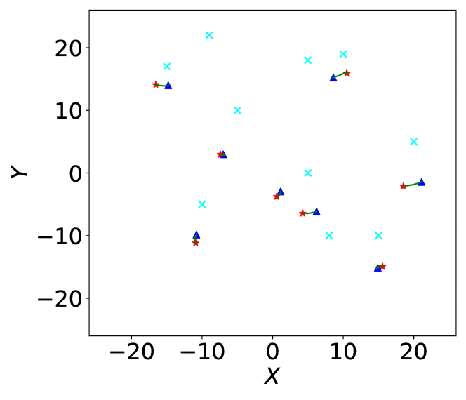
(a) update of sensor locations, $J=2000$

(b) objective value along iterations, $J=2000$

Figure 19: Allocation of 8 sensors for 10 emission sources ($\rho_{m}=0.00005$)

(a) update of sensor locations, $J=2000$

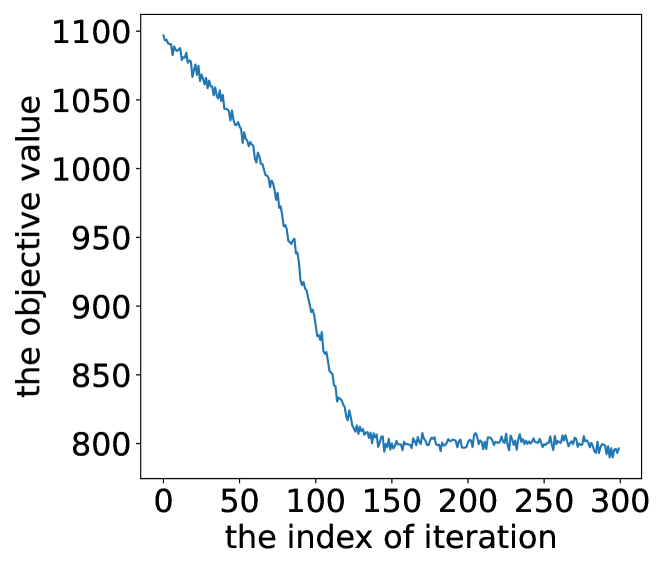
(b) objective value along iterations, $J=2000$

Figure 20: Allocation of 9 sensors for 10 emission sources ($\rho_{m}=0.00005$)

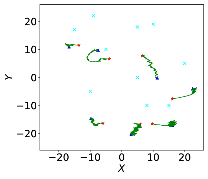
(a) update of sensor locations, $J=200$

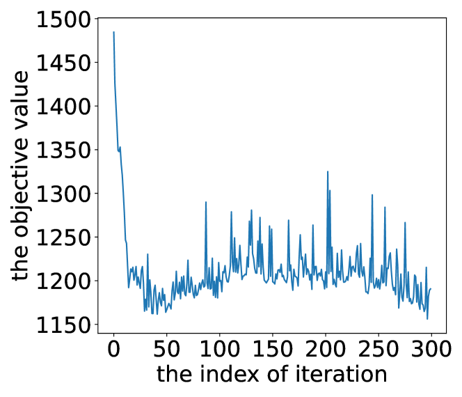
(b) objective value along iterations, $J=200$

Figure 21: Allocation of 7 sensors for 10 emission sources ($\rho_{m}=0.00005$).

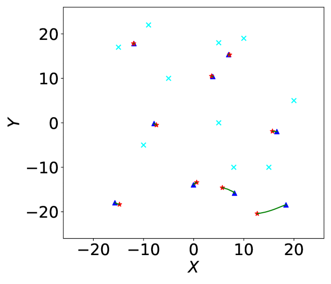
(a) update of sensor locations, $J=1$

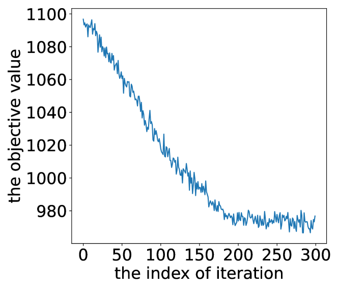
(b) objective value along iterations, $J=1$

Figure 22: Allocation of 9 sensors for 10 emission sources ($\rho_{m}=0.000001$).

(a) $J=2000$, $\rho_{m}=0.00005$, $M=300$

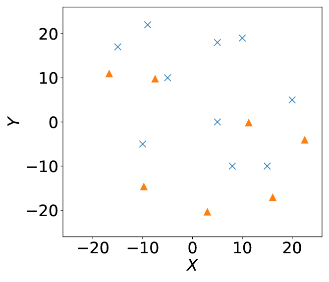
(b) $J=200$, $\rho_{m}=0.00005$, $M=300$

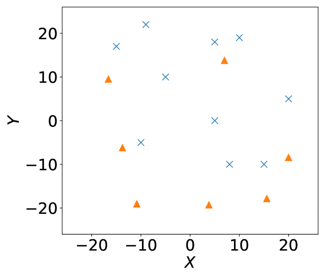
(c) $J=1$, $\rho_{m}=0.0000005$, $M=2000$

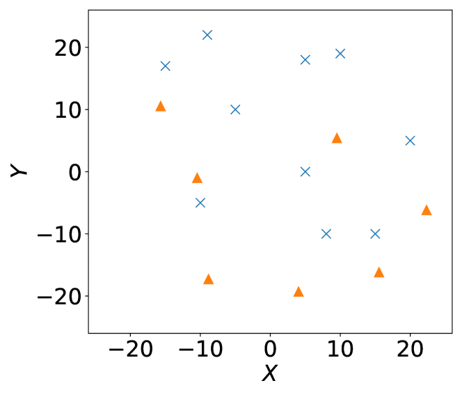
(d) $J=1$, $\rho_{m}=0.000001$, $M=3000$

Figure 23: Comparison of final designs between different hyperparameters (10 emission sources and 7 sensors, $N^{\prime}=20$)

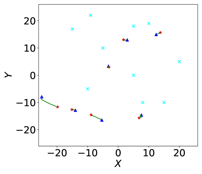
(a) update of sensor locations, $J=2000$

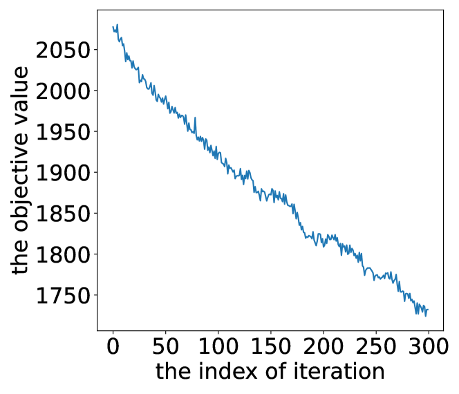
(b) objective value along iterations, $J=2000$

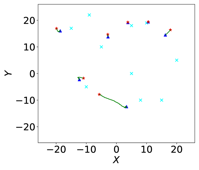
(c) update of sensor locations, $J=2000$

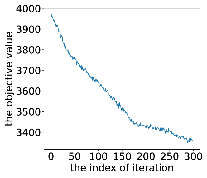
(d) objective value along iterations, $J=2000$

Figure 24: Initial sensor locations by random guess (10 emission sources and 7 sensors)

References

- [1] Gaussian plume model in matlab / python. https://personalpages.manchester.ac.uk/staff/paul.connolly/teaching/practicals/gaussian_plume_modelling.html.
- [2] A. Alexanderian, N. Petra, G. Stadler, and O. Ghattas, A-optimal design of experiments for infinite-dimensional bayesian linear inverse problems with regularized ell_0-sparsification, SIAM Journal on Scientific Computing, 36 (2014), pp. A2122–A2148.
- [3] A. Alexanderian and A. K. Saibaba, Efficient d-optimal design of experiments for infinite-dimensional bayesian linear inverse problems, SIAM Journal on Scientific Computing, 40 (2018), pp. A2956–A2985.
- [4] H. Antil, Z. W. Di, and R. Khatri, Bilevel optimization, deep learning and fractional laplacian regularization with applications in tomography, Inverse Problems, 36 (2020), p. 064001.
- [5] B. W. Brunton, S. L. Brunton, J. L. Proctor, and J. N. Kutz, Sparse sensor placement optimization for classification, SIAM Journal on Applied Mathematics, 76 (2016), pp. 2099–2122.
- [6] S. P. Chepuri and G. Leus, Continuous sensor placement, IEEE signal processing letters, 22 (2014), pp. 544–548.
- [7] F. K. Chow, B. Kosović, and S. Chan, Source inversion for contaminant plume dispersion in urban environments using building-resolving simulations, Journal of applied meteorology and climatology, 47 (2008), pp. 1553–1572.
- [8] B. M. de Silva, K. Manohar, E. Clark, B. W. Brunton, S. L. Brunton, and J. N. Kutz, Pysensors: A python package for sparse sensor placement, arXiv preprint arXiv:2102.13476, (2021).
- [9] S. Ghadimi and M. Wang, Approximation methods for bilevel programming, arXiv preprint arXiv:1802.02246, (2018).
- [10] T. Giovannelli, G. Kent, and L. N. Vicente, Inexact bilevel stochastic gradient methods for constrained and unconstrained lower-level problems, arXiv preprint arXiv:2110.00604, (2021).
- [11] G. H. Golub, P. C. Hansen, and D. P. O’Leary, Tikhonov regularization and total least squares, SIAM journal on matrix analysis and applications, 21 (1999), pp. 185–194.
- [12] E. Haber, L. Horesh, and L. Tenorio, Numerical methods for the design of large-scale nonlinear discrete ill-posed inverse problems, Inverse Problems, 26 (2009), p. 025002.
- [13] E. Haber, Z. Magnant, C. Lucero, and L. Tenorio, Numerical methods for a-optimal designs with a sparsity constraint for ill-posed inverse problems, Computational Optimization and Applications, 52 (2012), pp. 293–314.
- [14] J. L. Herring, J. G. Nagy, and L. Ruthotto, Lap: a linearize and project method for solving inverse problems with coupled variables, Sampling Theory in Signal and Image Processing, 17 (2018), pp. 127–151.
- [15] S. Houweling, T. Kaminski, F. Dentener, J. Lelieveld, and M. Heimann, Inverse modeling of methane sources and sinks using the adjoint of a global transport model, Journal of Geophysical Research: Atmospheres, 104 (1999), pp. 26137–26160.
- [16] X. Huan and Y. Marzouk, Gradient-based stochastic optimization methods in bayesian experimental design, International Journal for Uncertainty Quantification, 4 (2014).
- [17] X. Huan and Y. M. Marzouk, Simulation-based optimal bayesian experimental design for nonlinear systems, Journal of Computational Physics, 232 (2013), pp. 288–317.
- [18] Y. Hwang, E. Barut, and K. Yeo, Statistical-physical estimation of pollution emission, Statistica Sinica, 28 (2018), pp. 921–940.
- [19] Y. Hwang, H. J. Kim, W. Chang, K. Yeo, and Y. Kim, Bayesian pollution source identification via an inverse physics model, Computational Statistics & Data Analysis, 134 (2019), pp. 76–92.
- [20] S. Joshi and S. Boyd, Sensor selection via convex optimization, IEEE Transactions on Signal Processing, 57 (2008), pp. 451–462.
- [21] P. Khanduri, I. Tsaknakis, Y. Zhang, J. Liu, S. Liu, J. Zhang, and M. Hong, Linearly constrained bilevel optimization: A smoothed implicit gradient approach, (2023).
- [22] L. J. Klein, T. van Kessel, D. Nair, R. Muralidhar, H. Hamann, and N. Sosa, Monitoring fugitive methane gas emission from natural gas pads, in International Electronic Packaging Technical Conference and Exhibition, vol. 58097, American Society of Mechanical Engineers, 2017, p. V001T03A006.
- [23] K. A. Klise, B. L. Nicholson, and C. D. Laird, Sensor placement optimization using chama, tech. report, Sandia National Lab.(SNL-NM), Albuquerque, NM (United States), 2017.
- [24] A. Krause, A. Singh, and C. Guestrin, Near-optimal sensor placements in gaussian processes: Theory, efficient algorithms and empirical studies., Journal of Machine Learning Research, 9 (2008).
- [25] S. Liu and L. N. Vicente, The stochastic multi-gradient algorithm for multi-objective optimization and its application to supervised machine learning, Annals of Operations Research, (2021), pp. 1–30.
- [26] X. Liu and K. Yeo, Inverse models for estimating the initial condition of spatio-temporal advection-diffusion processes, Technometrics, (2023), pp. 1–14.
- [27] X. Liu, K. Yeo, L. Klein, Y. Hwang, D. Phan, and X. Liu, Optimal sensor placement for atmospheric inverse modelling, in 2022 IEEE International Conference on Big Data (Big Data), IEEE, 2022, pp. 4848–4853.
- [28] K. Manohar, B. W. Brunton, J. N. Kutz, and S. L. Brunton, Data-driven sparse sensor placement for reconstruction: Demonstrating the benefits of exploiting known patterns, IEEE Control Systems Magazine, 38 (2018), pp. 63–86.
- [29] K. Manohar, J. N. Kutz, and S. L. Brunton, Optimal sensor and actuator selection using balanced model reduction, IEEE Transactions on Automatic Control, 67 (2021), pp. 2108–2115.
- [30] M. Meng and X. Li, Aug-pdg: Linear convergence of convex optimization with inequality constraints, arXiv preprint arXiv:2011.08569, (2020).
- [31] L. Mustonen, X. Gao, A. Santana, R. Mitchell, Y. Vigfusson, and L. Ruthotto, A bayesian framework for molecular strain identification from mixed diagnostic samples, Inverse Problems, 34 (2018), p. 105009.
- [32] S. D. Narayanan, Z. B. Patel, A. Agnihotri, and N. Batra, A toolkit for spatial interpolation and sensor placement, in Proceedings of the 18th Conference on Embedded Networked Sensor Systems, 2020, pp. 653–654.
- [33] A. Nemirovski, A. Juditsky, G. Lan, and A. Shapiro, Robust stochastic approximation approach to stochastic programming, SIAM Journal on optimization, 19 (2009), pp. 1574–1609.
- [34] F. Parise and A. Ozdaglar, Sensitivity analysis for network aggregative games, in 2017 IEEE 56th Annual Conference on Decision and Control (CDC), IEEE, 2017, pp. 3200–3205.
- [35] J. Ranieri, A. Chebira, and M. Vetterli, Near-optimal sensor placement for linear inverse problems, IEEE Transactions on signal processing, 62 (2014), pp. 1135–1146.
- [36] L. Ruthotto, J. Chung, and M. Chung, Optimal experimental design for inverse problems with state constraints, SIAM Journal on Scientific Computing, 40 (2018), pp. B1080–B1100.
- [37] K. Schmidt, R. C. Smith, J. Hite, J. Mattingly, Y. Azmy, D. Rajan, and R. Goldhahn, Sequential optimal positioning of mobile sensors using mutual information, Statistical Analysis and Data Mining: The ASA Data Science Journal, 12 (2019), pp. 465–478.
- [38] A. Shapiro and A. Philpott, A tutorial on stochastic programming, Manuscript. Available at www2. isye. gatech. edu/ashapiro/publications. html, 17 (2007).
- [39] L. Sharrock and N. Kantas, Joint online parameter estimation and optimal sensor placement for the partially observed stochastic advection-diffusion equation, SIAM/ASA Journal on Uncertainty Quantification, 10 (2022), pp. 55–95.
- [40] J. Shen and T. F. Chan, Mathematical models for local nontexture inpaintings, SIAM Journal on Applied Mathematics, 62 (2002), pp. 1019–1043.
- [41] M. Sinsbeck and W. Nowak, Sequential design of computer experiments for the solution of bayesian inverse problems, SIAM/ASA Journal on Uncertainty Quantification, 5 (2017), pp. 640–664.
- [42] A. Spantini, T. Cui, K. Willcox, L. Tenorio, and Y. Marzouk, Goal-oriented optimal approximations of bayesian linear inverse problems, SIAM Journal on Scientific Computing, 39 (2017), pp. S167–S196.
- [43] J. M. Stockie, The mathematics of atmospheric dispersion modeling, Siam Review, 53 (2011), pp. 349–372.
- [44] A. Tarantola, Inverse problem theory and methods for model parameter estimation, SIAM, 2005.
- [45] I. Tsaknakis, P. Khanduri, and M. Hong, An implicit gradient-type method for linearly constrained bilevel problems, in ICASSP 2022-2022 IEEE International Conference on Acoustics, Speech and Signal Processing (ICASSP), IEEE, 2022, pp. 5438–5442.
- [46] Z. Wang, J. M. Bardsley, A. Solonen, T. Cui, and Y. M. Marzouk, Bayesian inverse problems with l_1 priors: a randomize-then-optimize approach, SIAM Journal on Scientific Computing, 39 (2017), pp. S140–S166.
- [47] R. A. Willoughby, Solutions of ill-posed problems (an tikhonov and vy arsenin), SIAM Review, 21 (1979), p. 266.
- [48] K. Wu, P. Chen, and O. Ghattas, An offline-online decomposition method for efficient linear bayesian goal-oriented optimal experimental design: Application to optimal sensor placement, SIAM Journal on Scientific Computing, 45 (2023), pp. B57–B77.
- [49] K. Yeo, Y. Hwang, X. Liu, and J. Kalagnanam, Development of hp-inverse model by using generalized polynomial chaos, Computer Methods in Applied Mechanics and Engineering, 347 (2019), pp. 1–20.
- [50] J. Yu, V. M. Zavala, and M. Anitescu, A scalable design of experiments framework for optimal sensor placement, Journal of Process Control, 67 (2018), pp. 44–55.
- [51] X. Zhao, K. Cheng, W. Zhou, Y. Cao, S.-h. Yang, and J. Chen, Source term estimation with deficient sensors: A temporal augment approach, Process Safety and Environmental Protection, 157 (2022), pp. 131–139.
- [52] H. Zou and T. Hastie, Regularization and variable selection via the elastic net, Journal of the Royal Statistical Society Series B: Statistical Methodology, 67 (2005), pp. 301–320.