A Novel Noise-Aware Classical Optimizer for Variational Quantum Algorithms

Abstract

A key component of variational quantum algorithms (VQAs) is the choice of classical optimizer employed to update the parameterization of an ansatz. It is well recognized that quantum algorithms will, for the foreseeable future, necessarily be run on noisy devices with limited fidelities. Thus, the evaluation of an objective function (e.g., the guiding function in the quantum approximate optimization algorithm (QAOA) or the expectation of the electronic Hamiltonian in variational quantum eigensolver (VQE)) required by a classical optimizer is subject not only to stochastic error from estimating an expected value but also to error resulting from intermittent hardware noise. Model-based derivative-free optimization methods have emerged as popular choices of a classical optimizer in the noisy VQA setting, based on empirical studies. However, these optimization methods were not explicitly designed with the consideration of noise. In this work we adapt recent developments from the “noise-aware numerical optimization” literature to these commonly used derivative-free model-based methods. We introduce the key defining characteristics of these novel noise-aware derivative-free model-based methods that separate them from standard model-based methods. We study an implementation of such noise-aware derivative-free model-based methods and compare its performance on demonstrative VQA simulations to classical solvers packaged in scikit-quant.

1 Introduction

Variational quantum algorithms (VQAs) form a class of quantum algorithms and are a leading method of experimentation for quantum computing researchers and practitioners [1]. VQAs have quantum circuit representations that are relatively simple and short and are therefore particularly well suited for near-term quantum computers, which have limited qubits and are prone to errors [2, 3]. The “variational” nature of VQAs comes from the manner in which VQAs combine classical optimization methods with quantum information techniques. The core idea behind VQAs is to use a quantum computer to evaluate a parameterized quantum circuit; the final quantum state returned by a VQA therefore depends on a given set of parameters. These parameters are adjusted by some classical numerical optimization algorithm that seeks the optimum of a well-designed and problem-specific cost function. VQAs have shown promise for solving binary optimization problems, for example, MaxCut variants [4, 5] and low autocorrelated binary sequences [6] problems, as well as for performing quantum simulations to identify ground state energies of complex molecules [7]. Their efficacy and flexibility have piqued the interest of researchers in chemistry [8, 9, 10], materials science [11], and machine learning [1].

In this manuscript we are particularly interested in the classical numerical optimization method that forms a critical part of a VQA. While some work suggests exploiting parameter shifts [12] to compute gradients with respect to the parameters, quantum circuits for computing these gradients are generally very large and hence far more prone to errors resulting from hardware noise. Some exploratory work in gradient-based classical optimizers for the VQA setting was performed by [13, 14, 15, 16, 17, 18]. However, in the near term where gate depths are prohibitive, the classical numerical optimization methods used to optimize VQA parameters will likely continue to have access only to cost function values. Given the complexity of the cost functions for these quantum systems, the employed optimization methods must be robust and efficient in navigating a landscape that is generally nonconvex and periodic [19]. This challenge, central to our motivations in this paper, is compounded by the fact that quantum measurements are inherently probabilistic; this means that the cost function values used in VQA are generally only statistical estimates. In particular, one is limited to sampling repeated measurements (called shots) of the output state of a quantum circuit; because most cost functions are expectations, a sample average of shot measurements typically yields an unbiased estimate of the cost function. However, these estimates necessarily introduce stochastic noise (in addition to, or separate from, any hardware noise) into the optimization process.

With the consideration of practically unattainable gradients, practitioners typically use methods for derivative-free optimization (DFO) [20] as the classical optimizer in a VQA. By derivative-free methods we refer to any optimization method that does not require any derivative information to be supplied by the user or the cost function oracle. For example, the software package scikit-quant [21] wraps a variety of derivative-free optimization solvers that the authors found to perform well on several benchmark variational quantum eigensolver (VQE) problems.

As discussed, the optimization problem solved on the classical computer is inherently stochastic. Despite this, the quantum computing community has largely found DFO methods that are explicitly for optimizing stochastic responses to be far less efficient than their counterparts for deterministic responses; for example, none of the solvers wrapped in scikit-quant are intended for stochastic optimization, by the standard definition of stochastic optimization. However, as is obvious in theory and is indeed observed in practice, any method designed for a deterministic problem will never resample a cost function at the same parameter setting twice. As a result, deterministic methods are certain to eventually “get stuck”; that is, they will fail to find improvement resulting from small perturbations of the circuit parameters. This “stuckness” is likely to happen when the noise becomes relatively large compared with the change in the cost function resulting from a parameter perturbation suggested by the methods.

Some of the most successful optimization methods for deterministic DFO problems (VQA or otherwise) are slight modifications to the model-based trust-region (MBTR) framework [22], with notable implementations having been developed by Michael Powell, including the popular BOBYQA [23]. MBTR methods construct and update a quadratic model of the objective function over a dynamically adjusted trust region, typically a norm ball of fixed radius in the parameter space. MBTR methods allow for efficient approximation of the overall objective function’s behavior, thereby guiding the optimization process more reliably, even in the absence of explicit gradient information. The method’s quadratic models are interpolatory; these models are especially useful when the signal from a noisy response is large relative to the noise. If the signal-to-noise ratio becomes small, however, the interpolatory models are likely not to model the response but rather provide a model of noise. In this low-signal setting, MBTR methods are likely to become stuck. However, MBTR methods empirically make reasonable progress for as long as the signal-to-noise ratio remains high.

In this work we seek to explicitly account for the observation that theoretically, and practically, MBTR methods perform best when the signal-to-noise ratio remains high. We accomplish this goal by developing what we call a noise-aware MBTR method. By noise-aware, we broadly refer to any method that effectively requires an estimate of the noise level present in the function evaluation. We currently leave the meaning of noise level intentionally vague, but for intuition, noise level could refer to any of the following:

• a deterministic bound on the absolute value of noise,

• the standard error when one employs sample means to estimate an expectation value, or

• the noise level of a deterministically noisy function, as employed in [24],

among other quantities. We note in particular that we do not label our method a stochastic MBTR because, for instance, of the three examples presented above, only the second example assumes anything stochastic about the function being estimated. In the VQA setting, this choice is motivated by the practical concern that observations of circuit evaluations on a near-term quantum computer are the result not only of a stochastic calculus but also of hardware noise. There is generally no reason to believe that hardware noise satisfies distributional assumptions as pleasant as unbiasedness or parameter independence. Moreover, from a theoretical perspective, the analysis of stochastic optimization methods tends to focus on (non)asymptotic convergence rates as a primary concern. For convergence analyses of various stochastic MBTR methods, see, for example, [25, 26, 27, 28, 29, 30]. All of these methods effectively assume that, in the presence of stochastic noise, one must sample the objective function in each iteration $k$ at a rate like $\mathcal{O}(1/\Delta_{k}^{4})$, where $\Delta_{k}$ is a trust-region radius. Because the theoretical convergence of an MBTR method requires $\Delta_{k}\to 0$, this sampling rate can quickly become infeasible in practice. As a result, the stochastic optimization methods suggested by these analyses focus on long-term convergence, often at the expense of efficiency in the number of function evaluations spent while satisfying a fixed budget.

Therefore, we seek to provide the best possible theoretical convergence results for a noise-aware MBTR method. We aim to achieve this by building on recent results in what we would call noise-aware optimization. Of particular note are [31] and [32], which provide convergence analyses for trust-region frameworks given explicit access to an estimate of a noise level. The definitions of “noise level” differ between these two reference works; we believe that the framework in [32] provides a bit more flexibility that allows the results to be especially appropriate in the VQA setting. The results of both [31] and [32] can be characterized as providing a neighborhood of convergence for an optimization method given a reasonable estimate of the noise level. Thus, instead of trying to achieve arbitrary accuracy (which, for instance, would require an insurmountable number of samples in a stochastic setting), the analysis provides a worst-case rate of convergence to a solution of “best possible” accuracy, given the noise level. The primary achievement of this manuscript is to take the noise-aware trust-region framework of [32] and, through careful consideration of interpolation model construction, yield a practical implementation of a noise-aware MBTR method. The convergence of our method will follow immediately by algorithmically ensuring that the interpolation models satisfy certain properties that are assumed in [32].

The outline of the manuscript is as follows. Section 2 develops the problem setting, and Section 2.1 discusses the chosen noise model suitable for VQAs. Section 2.2 presents a general noise-aware trust-region algorithm from the literature that we will build upon, and Section 2.3 presents some of its theoretical properties. Section 3 presents our novel method for noise-aware optimization, and Section 4 analyzes the convergence properties of its sequence of iterates. Section 5 presents numerical results for our novel algorithm on a selection of noisy optimization problems. Section 6 concludes with open questions for further investigation.

2 Setting

Given a computational ansatz, let a quantum circuit be parameterized by $\theta\in\mathcal{R}^{d}$. We aim to solve the optimization problem

$$\text{minimize}f(\theta):\theta\in\mathcal{R}^{d},$$ (1)

where $f:\mathcal{R}^{d}\to\mathcal{R}$ denotes some objective function (e.g., a guiding function in QAOA or the energy of the Hamiltonian in VQE).

We first discuss, in Section 2.1, a particular choice of noise model from recent literature that appears to be appropriate for the noisy VQA setting. A suitable trust-region algorithm for the minimization of objective functions subscribing to this noise model was also recently proposed, and we present it in Section 2.2. In Section 2.3 we summarize results concerning the asymptotic performance of this trust-region algorithm.

2.1 A Noise Model

Motivated by the role of the classical optimizer in the VQA setting, we consider a noise setting similar to that investigated in Cao et al. [32]. In particular, we suppose that our access to an underlying objective function $f:\mathcal{R}^{d}\to\mathcal{R}$ is through what Cao et al. [32] refers to as a “stochastic zeroth-order oracle” (of one of two types):

Definition 1.

Let $\xi$ denote a random variable that may or may not depend on the optimization variables $\theta$. We say $\tilde{f}(\theta,\xi)$ is a zeroth-order oracle for $f$ provided for all $x\in\mathcal{R}^{d}$, the error quantity

$$e(\theta,\xi)=\tilde{f}(\theta,\xi)-f(\theta)$$ (2)

satisfies at least one of two conditions:

Type 1. (Deterministically bounded noise)

There exists a constant $\epsilon_{f}\geq 0$ such that $|e(\theta,\xi)|\leq\epsilon_{f}$ for all realizations of $\xi$.

Type 2. (Independent subexponential noise)

There exist constants $\epsilon_{f}\geq 0$ and $c>0$ such that

$$\mathbb{P}_{\xi}\left[|e(\theta,\xi)|>t\right]\leq\exp(c(\epsilon_{f}-t))\quad\forall t\geq 0.$$ (3)

We remark that the random variable $\xi$ in Definition 1 should be considered exogenous in the sense that an optimization algorithm accessing $\tilde{f}$ cannot provide an input $\xi$. Hence, for ease of notation, we will denote the noisy evaluations of $f$ as $\tilde{f}(\theta)$ throughout this manuscript. We additionally remark that while, for generality, Definition 1 is stated in terms of random variables, the definition does not preclude noisy deterministic functions; in that case, one can trivially assign some Dirac distribution to $\xi$, and the definition is still meaningful. To provide context, one can interpret eq. 3 as saying that the errors exhibit a subexponential tail (with rate determined by $c$); moreover, eq. 3 suggests that there are no restrictions on the distribution of errors of magnitude within $\epsilon_{f}$. Many commonly used and naturally occurring probability distributions fall within this definition.

We believe the assumption that a quantum computer’s output exhibits the properties of a zeroth-order oracle is reasonable. For example, in QAOA, a single shot of the output of the quantum circuit corresponds to one of combinatorially many binary vectors, which are then evaluated through the objective function of a combinatorial optimization problem on the classical device. The objective function used by the classical optimizer, in turn, is essentially an average of Bernoulli variables (one variable for each binary solution) weighted by the original combinatorial problem’s objective values. If one supposes that the combinatorial problem is well defined, and because Bernoulli variables have bounded (finite) support, the error $\epsilon_{f}$ is always trivially deterministically bounded in QAOA and is a Type 1 error as we have defined.

Of course, such a trivial deterministic bound is loose to the point of uselessness. However, using Bernstein inequality, one can show that the distribution of errors of the finitely supported $\tilde{f}$ will yield $c$ in eq. 3 that scales linearly in the shot count (that is, the subexponential rate of decay is proportionally faster). Under this interpretation, $\epsilon_{f}$ is the population standard deviation $\sigma$ for the distribution described by $\tilde{f}(\theta)$.

We are additionally attracted to the noise model defined in Definition 1 in the VQA setting because of its nonparametric flexibility. The definition itself does not specify what the noise distribution ought to be but essentially assumes (via Bernstein inequality) only that the variance of $\tilde{f}(\theta)$ is defined and that there exist bounds on higher moments of $\tilde{f}(\theta)$.

We also find this noise model attractive for VQA because of intermittent hardware noise, which remains a salient difficulty in near-term quantum devices. Owing to the nonparametric assumption, even if a quantum device “drifts” over time [33], the noise model is sufficiently flexible to describe a sum of stochastic error (as previously discussed) and hardware error. While the “variance” (and higher moments) of hardware noise is not easily quantifiable, allowing a sufficiently large $\epsilon_{f}$ in the deterministically bounded regime of Definition 1 can potentially encapsulate hardware noise. This interpretation lends credence to the use and purported convergence guarantees of algorithms based on zeroth-order oracles, like the one we will describe now.

2.2 A Noise-Aware Trust-Region Algorithmic Framework

We begin by restating the general first-order trust-region algorithm of Cao et al. [32][Algorithm 1] in Algorithm 1; our statement is identical up to changes in notation. For a complete statement of Algorithm 1, we require one additional definition, which must be carefully handled in derivative-free optimization.

Definition 2.

Let $\xi$ denote a random variable. We say $g(\theta,\xi)$ is a first-order oracle for $\nabla f(\theta)$ provided there exist $\kappa_{eg}\geq 0$ and $\epsilon_{g}\geq 0$ such that for any given $\theta\in\mathcal{R}^{d}$, for any given $\Delta>0$, and for any given probability $p_{1}\in[0.5,1]$,

$$\mathbb{P}_{\xi}\left[\|g(\theta,\xi)-\nabla f(\theta)\|\leq\epsilon_{g}+\kappa_{eg}\Delta\right]\geq p_{1}.$$ (4)

The random variable $\xi$ may or may not depend on $\theta$ and $\Delta$.

Given access to a zeroth-order oracle (see Definition 1) and a first-order oracle (see Definition 2), convergence results for Algorithm 1 may be proven.

Input: starting point $\theta_{0}$; initial trust-region radius $\Delta_{0}>0$; trust-region parameters $\eta_{1},\eta_{2},\gamma\in(0,1)$, tolerance parameter $r\geq 2\epsilon_{f}$, probability parameter $p_{1}$, bound on model Hessians $\kappa_{\text{bmh}}\geq 0$, constant $\kappa_{\mathrm{fcd}}\in(0,1]$

1 Evaluate $\tilde{f}(\theta)$ if not previously evaluated.

2for $k=0,1,2,\ldots$ do

3       Compute model gradient $g_{k}$ via first-order oracle with input $\theta_{k},p_{1},$ and $\Delta_{k}$

4      Let $H_{k}$ be a model Hessian satisfying $\|H_{k}\|\leq\kappa_{\text{bmh}}$

5      Construct a local quadratic model

$$m_{k}(s)=\tilde{f}(\theta_{k})+g_{k}^{T}s+s^{T}H_{k}s$$ (5)

6      Compute $s_{k}$ as an approximate minimizer of $\{\min m_{k}(s):s\in\mathcal{B}(0,\Delta_{k})\}$, such that $s_{k}$ satisfies

$$m_{k}\left(\theta_{k}\right)-m_{k}\left(\theta_{k}+s_{k}\right)\geq\frac{\kappa_{\mathrm{fcd}}}{2}\left\|g_{k}\right\|\min\left\{\frac{\left\|g_{k}\right\|}{\left\|H_{k}\right\|},\Delta_{k}\right\}$$ (6)

7      Evaluate $\tilde{f}(\theta_{k}+s_{k})$ from zeroth-order oracle as in Definition 1.

8      Compute

$$\rho_{k}=\frac{\tilde{f}(\theta_{k})-\tilde{f}(\theta_{k}+s_{k})+r}{m_{k}\left(0\right)-m_{k}\left(s_{k}\right)}$$ (7)

if $\rho_{k}\geq\eta_{1}$ then

9            

$$\mbox{Set $\theta_{k+1}=\theta_{k}+s_{k}$ and }\Delta_{k+1}=\begin{cases}\gamma^{-1}\Delta_{k}&\text{ if }\left\|g_{k}\right\|\geq\eta_{2}\Delta_{k}\\ \gamma\Delta_{k},&\text{ if }\left\|g_{k}\right\|<\eta_{2}\Delta_{k}\end{cases}$$

10      else

11             Set $\theta_{k+1}=\theta_{k}$ and $\Delta_{k+1}=\gamma\Delta_{k}$.

12      

Algorithm 1 General framework for noise-aware optimization

2.3 Preliminary Assumptions and Analysis

Under reasonable assumptions, Cao et al. [32][Theorems 4.11 and 4.18] demonstrate that in both the deterministically bounded noise regime and the subexponential noise regime, the probability of exceeding $\mathcal{O}(1/\epsilon^{2})$ iterations of Algorithm 1 to find an $\epsilon$-stationary solution to eq. 1 decays exponentially in the exceedance; $\epsilon$ is a function of $\epsilon_{f}$ and $\epsilon_{g}$.

We start by making the following assumptions.

Assumption 1.

The objective function $f$ is continuously differentiable. That is, the gradient $\nabla f$ is $L_{\nabla f}$-Lipschitz continuous on $\mathcal{R}^{d}$ and satisfies

$$\|\nabla f(\theta^{(1)})-\nabla f(\theta^{(2)})\|\leq L_{\nabla f}\|\theta^{(1)}-\theta^{(2)}\|$$

for all $(\theta^{(1)},\theta^{(2)})\in\mathcal{R}^{d}\times\mathcal{R}^{d}$.

Assumption 2.

The function $f$ is lower bounded by $f_{\inf}$.

Assumption 3.

For all $k=0,1,\cdots$, $\|H_{k}\|\leq\kappa_{\mathrm{bhm}}$, where $\kappa_{\mathrm{bhm}}>0$.

We state intentionally simplified versions of two main results of Cao et al. [32], which provide the number of iterations $T$ needed to ensure (with high probability) that within the first $T$ iterations, the event $\left\{\left\|\nabla f\left(\theta_{k}\right)\right\|\leq\epsilon\right\}$ occurs.

Theorem 1.

Suppose Assumptions 1–3 are satisfied. Suppose we have access to a zeroth-order oracle of Type 1 with parameter $\epsilon_{f}$ and a first-order oracle with parameters $\kappa_{eg},\epsilon_{g},$ and $p_{1}$. Let $\{\Theta_{k}\}$ denote the sequence of random variables with realizations $\{\theta_{k}\}$ generated by Algorithm 1. There exists $\kappa$, independent of $\epsilon_{f},\epsilon_{g},p_{1}$ but dependent on $\kappa_{eg}$, such that given any

$$\epsilon>\kappa\left(\sqrt{\frac{\epsilon_{f}}{2p_{1}-1}}+\epsilon_{g}\right),$$

it holds that

$$\mathbb{P}\left[\displaystyle\min_{0\leq k\leq T-1}\|\nabla f(\Theta_{k})\|\leq\epsilon\right]\geq 1-\exp\left(-\mathcal{O}(T)\right)$$

for any $T\in\mathcal{O}\left(\frac{1}{\epsilon^{2}}\right)$.

Theorem 2.

Suppose that Assumptions 1–3 are satisfied. Suppose we have access to a zeroth-order oracle of Type 2 with parameters $\epsilon_{f}$ and $c$ and a first-order oracle with parameters $\kappa_{eg},\epsilon_{g},$ and $p_{1}$. Define $p_{0}=1-2\exp(c(\epsilon_{f}-r/2))$. Let $\{\Theta_{k}\}$ denote the sequence of random variables with realizations $\{\theta_{k}\}$ generated by Algorithm 1. There exists $\kappa$, independent of $\epsilon_{f},\epsilon_{g},p_{1}$ but dependent on $\kappa_{eg}$, such that given any

$$\epsilon>\kappa\left(\sqrt{\frac{\epsilon_{f}+1/c}{2p_{0}+2p_{1}-3}}+\epsilon_{g}\right),$$

it holds that

$$\mathbb{P}\left[\displaystyle\min_{0\leq k\leq T-1}\|\nabla f(\Theta_{k})\|\leq\epsilon\right]\geq 1-2\exp\left(-\mathcal{O}(T)\right)-\exp\left(-ct/4\right)$$

for any $T\in\mathcal{O}\left(\frac{1}{\epsilon^{2}}\right)$ and any $t>0$.

Remark 1.

While we encourage the reader to study Cao et al. [32][Theorems 4.11 & 4.18] for a complete description of the constants that we have deliberately hidden in $\mathcal{O}(T)$ and $\mathcal{O}(1/\epsilon^{2})$, we remark that, as one might intuit, the $\mathcal{O}(T)$ rate in the exponentially decaying probability decreases in $\epsilon_{f}$, and the $\mathcal{O}\left(\frac{1}{\epsilon^{2}}\right)$ term increases with both the initial optimality gap $f(\theta_{0})-f_{\inf}$ and the Lipschitz constant $L_{\nabla f}$. When $\epsilon_{f}=\epsilon_{g}=0$, Theorem 1 reduces to something resembling the first-order convergence result for a standard derivative-free trust-region algorithm; see, for example, Conn et al. [22][Chapter 10].

3 A Practical Noise-Aware Derivative-Free Algorithm Based on Algorithm 1

While Algorithm 1 provides an invaluable framework for analyzing DFO methods, it does not lend itself immediately to a practical algorithm for DFO. In particular, Algorithm 1 does not detail how to construct a first-order oracle for computing $g_{k}$ or how to choose model Hessians $H_{k}$. Cao et al. [32] suggest using linear interpolation of noisy function values for the first-order oracle, similar to the approach analyzed by Berahas et al. [34]. Our approach aligns with this line of reasoning but is further motivated by two practical considerations. First, we aim to go beyond linear interpolation models to also minimum Frobenius norm quadratic interpolation models. (This extension is certainly not new and is the subject of Conn et al. [22][Chapter 5].) Second, and more important, because we often employ model-based methods for optimizing computationally expensive objectives in derivative-free optimization, we do not want to generate a new set of interpolation points on every iteration. Rather, we prefer to judiciously reuse previously evaluated points and their corresponding (noisy) function evaluations. Especially in the noisy setting, this merits a careful reexamination of known results concerning the geometry of interpolation sets and algorithmic methods for ensuring geometric constraints are satisfied in practice. In addition, we impose a lower bound on a sampling radius when we select points for model construction, in order to ensure that the error between the true gradient and the model gradient is controlled. Section 3.1 focuses on precisely establishing these algorithmic controls.

3.1 Geometry of Interpolation Sets

At every iteration $k\in\{0,1,\dots\}$ of our derivative-free trust-region algorithm, there exists an incumbent iterate $\theta_{k}$ (that is also a trust-region center). In each iteration, a set of distinct points $\mathcal{X}=\{x^{0}=\theta_{k},x^{1},\cdots,x^{p}\}\subset\mathcal{R}^{d}$ is selected; the algorithm ensures that the noisy function $\tilde{f}$ is evaluated at each $x\in\mathcal{X}$. A model is constructed such that it interpolates the noisy function $\tilde{f}$ at each $x\in\mathcal{X}$, and this model is intended to approximate the objective function near $\theta_{k}$.

In this work we will focus on minimum Frobenius norm quadratic interpolation models, which are appropriate in the setting of budget-constrained (expensive) derivative-free optimization. We consider the space of all quadratic polynomials in $\mathcal{R}^{d}$; a suitable basis for this space is given by the union of the degree-zero and degree-one monomials $\{1,x_{1},x_{2},\dots,x_{d}\}$ and the degree-two monomials $\{x_{1}^{2},\dots,x_{d}^{2},x_{1}x_{2},x_{1}x_{3},\dots,x_{1}x_{n},\dots,x_{n-1}x_{n}\}$. Vectorizing these two sets as $\mu(x)\in\mathcal{R}^{d+1}$ and $\nu(x)\in\mathcal{R}^{d(d+1)/2}$ respectively, we see that any degree-two polynomial, and hence any quadratic interpolation model, can be expressed as

$$m(x)=\alpha^{T}\mu(x)+\beta^{T}\nu(x),$$ (8)

for $\alpha\in\mathcal{R}^{d+1}$ and $\beta\in\mathcal{R}^{d(d+1)/2}$.

We assume throughout that the interpolation set $\mathcal{X}$ has cardinality $p\in[d+1,(d+1)(d+2)/2]$. Define

$$\tilde{f}(\mathcal{X})=\left[\begin{array}[]{r}\tilde{f}\left(x^{0}\right),\tilde{f}\left(x^{1}\right),\dots,\tilde{f}\left(x^{p}\right)\end{array}\right]^{\top},$$ (9)

where $\tilde{f}\left(x^{i}\right)$ represents noisy evaluations of $f\left(x^{i}\right)$ for $i=0,1,\dots,p$. Enforcing $m(x^{i})=\tilde{f}(x^{i})$ for $i=0,1,\dots,p$ is tantamount to solving

$$\left[\begin{array}[]{l}M_{\mathcal{X}}\\ N_{\mathcal{X}}\end{array}\right]^{T}\left[\begin{array}[]{l}\alpha\\ \beta\end{array}\right]=\tilde{f}(\mathcal{X}),$$ (14)

where we define $M_{\mathcal{X}}\in\mathcal{R}^{(d+1)\times|\mathcal{X}|}$ and $N_{\mathcal{X}}\in\mathcal{R}^{d(d+1)/2\times|\mathcal{X}|}$, by $M_{i,j}=\mu_{i}\left(x^{j}\right)$ and $N_{i,j}=\nu_{i}\left(x^{j}\right)$, respectively. Note that eq. 14 may not admit a unique solution since $|\mathcal{X}|\leq(d+1)(d+2)/2$. We will focus on solutions to the interpolation problem eq. 14 that are of minimum norm with respect to the vector $\beta$. That is, we seek $(\alpha,\beta)$ that solve

$$\min\left\{\frac{1}{2}\|\beta\|^{2}:M_{\mathcal{X}}^{T}\alpha+N_{\mathcal{X}}^{T}\beta=\tilde{f}(\mathcal{X})\right\}.$$ (15)

The solution to eq. 15 is a quadratic polynomial whose Hessian matrix is of minimum Frobenius norm, since $\|\beta\|=\left\|\nabla_{xx}^{2}m(x)\right\|_{F}$. The KKT conditions for eq. 15 can be written as

$$\left[\begin{array}[]{cc}N_{\mathcal{X}}^{T}N_{\mathcal{X}}&M_{\mathcal{X}}^{T}\\ M_{\mathcal{X}}&0\end{array}\right]\left[\begin{array}[]{l}\lambda\\ \alpha\end{array}\right]=\left[\begin{array}[]{c}\tilde{f}(\mathcal{X})\\ 0\end{array}\right]$$ (22)

with $\beta=N_{\mathcal{X}}\lambda$. We make the observation that to guarantee eq. 22 will yield a unique solution, we must have that both $rank(M_{\mathcal{X}})=d+1$ and $N_{\mathcal{X}}^{T}N_{\mathcal{X}}$ is positive definite for all $u\in\mathcal{R}^{d}$ such that $M_{\mathcal{X}}u=0$.

Although relatively expensive compared with, for instance, the heuristic employed in POUNDers (see Wild [35] for details), we find that careful geometry maintenance is critical to the performance of a derivative-free model-based optimization method in the noisy setting. Recalling Definition 1, we aim to ensure that, given $\Delta>0$, the model gradient $g$ defined by $\alpha$ in eq. 8 satisfies eq. 4 for some values of $\epsilon_{g},\kappa_{eg},$ and $p_{1}$. Demonstrating such a result requires careful consideration of the geometry of $\mathcal{X}$. We begin by introducing the concept of Lagrange polynomials associated with $\mathcal{X}$.

Definition 3.

Given a set $\mathcal{X}=\{x^{0},x^{1},\dots,x^{p}\}\subset\mathcal{R}^{d}$ of interpolation points, we define the minimum Frobenius norm Lagrange polynomials associated with $\mathcal{X}$ as the set of polynomials $\{\ell_{i}(x)=\alpha_{i}^{\top}\mu(x)+\beta_{i}^{\top}\nu(x):i=0,1,\dots,p\}$ with coefficients $(\alpha_{i},\beta_{i})$ chosen such that, for each $i$, $(\alpha_{i},\beta_{i})$ is the solution to eq. 15 when the function $f$ in the right-hand side in the constraint is replaced with the indicator function for $x^{i}$.

It is straightforward to demonstrate that the minimum Frobenius norm model $m(x)$ in eq. 8 is expressible via a linear combination of minimum Frobenius norm Lagrange polynomials, that is,

$$m(x)=\displaystyle\sum_{i=0}^{p}f(x^{i})\ell_{i}(x).$$ (23)

Moreover, denoting the matrix in the left-hand side of eq. 22 by $W_{\mathcal{X}}$, it is clear from the definition of minimum Frobenius norm Lagrange polynomials that each $(\alpha_{i},\beta_{i})$ defining the polynomials may be computed directly from the columns of $W_{\mathcal{X}}^{-1}$. In particular, the last $d+1$ entries of the $i$th column of $W_{\mathcal{X}}^{-1}$ define $\alpha_{i}$. Also, by considering the constraints in the quadratic dual program to eq. 15, one may derive that the quadratic term of $\ell_{i}(x)$ described by $\beta_{i}$ is a weighted sum of rank-one matrices,

$$\nabla^{2}\ell_{j}(x)=\displaystyle\sum_{j=0}^{p}\left[W_{\mathcal{X}}^{-1}\right]_{j+1,i}(x^{i}-x^{0})(x^{i}-x^{0})^{\top}.$$

With computable expressions for the minimum Frobenius norm Lagrange polynomials associated with a set $\mathcal{X}$ in hand, the following definition of $\Lambda$-poisedness is easily stated.

Definition 4.

We say that $\mathcal{X}$ is poised in the minimum Frobenius norm sense provided $W_{\mathcal{X}}$ is nonsingular.

Definition 5.

Let $\Lambda>0$, and let a set $B\subset\mathcal{R}^{d}$ be given. A set $\mathcal{X}=\{x^{0},x^{1},\dots,x^{p}\}$, poised in the minimum Frobenius norm sense, is moreover $\Lambda$-poised in $B$ in the minimum Frobenius norm sense provided

$$\Lambda\geq\displaystyle\max_{0,1,\dots,p}\displaystyle\max_{x\in B}|\ell_{i}(x)|.$$

Critical to our development of error bounds, we state the following results.

Theorem 3.

Let $\Lambda>0$, and let $\mathcal{X}=\{x^{0},x^{1},\dots,x^{p}\}$ be a given set of interpolation points. Let $\mathcal{B}(x^{0},\Delta)\subset\mathcal{R}^{d}$ be a ball sufficiently large such that $\mathcal{X}\subset\mathcal{B}(x^{0},\Delta)$. Suppose Assumption 1 holds with constant $L_{\nabla f}$. Define the matrix

$$\hat{L}=\frac{1}{\Delta}\left[\begin{array}[]{cccc}x^{1}-x^{0}&x^{2}-x^{0}&\cdots&x^{p}-x^{0},\\ \end{array}\right]^{\top}$$

and denote its pseudoinverse via $\hat{L}^{\dagger}=(\hat{L}^{\top}\hat{L})^{-1}\hat{L}^{\top}$. Define

$$\epsilon_{\max}=\displaystyle\max_{i=1,2,\dots,p}|\tilde{f}(x^{i})-f(x^{i})|\quad\text{ and }\quad\epsilon_{0}=|\tilde{f}(x^{0})-f(x^{0})|.$$

If $\mathcal{X}$ is $\Lambda$-poised in $\mathcal{B}(x^{0},\Delta)$ in the minimum Frobenius norm sense, then the minimum Frobenius norm model $m(x)$ satisfies

$$\|\nabla f(x)-\nabla m(x)\|\leq\sqrt{p+1}\|\hat{L}^{\dagger}\|\left[(L_{\nabla f}+\|\nabla^{2}m(x^{0})\|)\Delta+\frac{\epsilon_{0}+\epsilon_{\max}}{\Delta}\right]\quad\forall x\in\mathcal{B}(x^{0},\Delta).$$

Proof.

For ease of notation, we denote the quadratic underdetermined interpolation model $m(x)$ as

$$m(x)=c+g^{\top}x+\frac{1}{2}x^{\top}Hx.$$

In other words, we have simply reorganized the terms in eq. 8. For an arbitrary point $x\in\mathcal{B}(x^{0},\Delta)$, denote the function value error ($e^{f}$) and the gradient value error ($e^{g}$) via

$$m(x)=f(x)+e^{f}(x)\quad\text{ and }\quad\nabla m(x)=Hx+g=\nabla f(x)+e^{g}(x).$$

Because $m(x)$ interpolates $\tilde{f}(x)$ at each point in $\mathcal{X}$, we conclude from the expression for $e^{f}$ that, for each $i=0,1,\dots,p$,

$$\begin{array}[]{rll}m(x^{i})&=\tilde{f}(x^{i})&\iff\\ c+g^{\top}x^{i}+\frac{1}{2}x^{i\top}Hx^{i}&=\tilde{f}(x^{i})&\iff\\ c+g^{\top}x^{i}+\frac{1}{2}x^{i\top}Hx^{i}-m(x)&=\tilde{f}(x^{i})-m(x)&\iff\\ (x^{i}-x)^{\top}g+\frac{1}{2}(x^{i}-x)^{\top}H(x^{i}-x)+(x^{i}-x)^{\top}Hx&=\tilde{f}(x^{i})-f(x)-e^{f}(x).\end{array}$$

Now, substituting in the expression for $e^{g}$, we have for each $i=0,1,\dots,p$

$$(x^{i}-x)^{\top}(e^{g}(x)+\nabla f(x))+\frac{1}{2}(x^{i}-x)^{\top}H(x^{i}-x)=\tilde{f}(x^{i})-f(x)-e^{f}(x).$$

Trivially, we also have

$$(x^{i}-x)^{\top}(e^{g}(x)+\nabla f(x))+\frac{1}{2}(x^{i}-x)^{\top}H(x^{i}-x)=\tilde{f}(x^{i})-f(x)-e^{f}(x)+f(x^{i})-f(x^{i}).$$

By Taylor’s theorem and the definition of $\Delta$, $f(x)+\nabla f(x)^{\top}(x^{i}-x)-f(x^{i})\in\mathcal{O}(\Delta^{2})$. Thus there exists $c_{i}\in\mathcal{R}$ independent of $\Delta$ such that, for all $i=0,1,\dots,p$,

$$(x^{i}-x)^{\top}e^{g}(x)+\frac{1}{2}(x^{i}-x)^{\top}H(x^{i}-x)=c_{i}\Delta^{2}-e^{f}(x)+\tilde{f}(x^{i})-f(x^{i}).$$ (24)

Now, subtracting eq. 24 for $i=0$ from each of eq. 24 for $i=1,\dots,p$, we get for $i=1,\dots,p$ that

$$(x^{i}-x^{0})^{\top}e^{g}(x)+\frac{1}{2}(x^{i}-x)^{\top}H(x^{i}-x)-\frac{1}{2}(x^{0}-x)^{\top}H(x^{0}-x)=(c_{i}-c_{0})\Delta^{2}+\tilde{f}(x^{i})-f(x^{i})-\tilde{f}(x^{0})+f(x^{0}).$$

It now follows from the assumptions on $f$ and $\tilde{f}$ and the definitions of $\Delta,\hat{L}^{\dagger},\epsilon_{\max}$ and $\epsilon_{0}$ that

$$\|e^{g}(x)\|\leq\sqrt{p+1}\|\hat{L}^{\dagger}\|\left[\left(L_{\nabla f}+\|H\|\right)\Delta+\left(\frac{\epsilon_{0}+\epsilon_{\max}}{\Delta}\right)\right].$$

∎

In order to extract a meaningful bound from Theorem 3, it remains to bound both the quantities $\|\hat{L}^{\dagger}\|$ and $\|\nabla^{2}m(x^{0})\|$ appearing in Theorem 3. The former quantity can be bounded by observations made in the development of Conn et al. [22][Section 5.3]. The proof of these observations involves an alternative characterization of Definition 5 that we will not provide in this manuscript for the sake of concise exposition; see Conn et al. [22][Section 5.3] for full details. We state this bound on $\|\hat{L}^{\dagger}\|$ in Proposition 1. The quantity $\|\nabla^{2}m(x^{0})\|$ can be bounded by mimicking the proof of a result in Conn et al. [22][Theorem 5.7]. We state and prove that bound in Theorem 4.

Proposition 1.

Let $\mathcal{X}$ be $\Lambda$-poised in the minimum Frobenius norm sense. Let Assumption 1 hold. Then, $\hat{L}^{\dagger}$ in the statement of Theorem 3 automatically satisfies

$$\|\hat{L}^{\dagger}\|\leq\sqrt{p+1}\Lambda.$$

Theorem 4.

Let $\Lambda>0$, and let $\mathcal{X}=\{x^{0},x^{1},\dots,x^{p}\}$ be a given set of interpolation points. Denote the absolute error in function value at each interpolation point by $\epsilon_{i}=|e(x^{i},\xi_{i})|.$ Let $\mathcal{B}(x^{0},\Delta)\subset\mathcal{R}^{d}$ be a ball sufficiently large such that $\mathcal{X}\subset\mathcal{B}(x^{0},\Delta)$. Suppose $f$ is continuously differentiable in an open set $\Omega$ such that $\mathcal{B}(x^{0},\Delta)\subset\Omega$, and suppose $\nabla f$ is Lipschitz continuous in $\Omega$ with constant $L_{\nabla f}$. Then,

$$\|\nabla^{2}m(x^{0})\|\leq\displaystyle\frac{4(p+1)\Lambda L_{\nabla f}\sqrt{(d+1)(d+2)}}{\nu(\Delta)}+\displaystyle\frac{8\Lambda\sqrt{(d+1)(d+2)}}{\Delta^{2}\nu(\Delta)}\sum_{i=0}^{p}\epsilon_{i},$$ (25)

where we have denoted

$$\nu(\Delta)=\min\left\{1,\frac{1}{\Delta},\frac{1}{\Delta^{2}}\right\}.$$ (26)

Proof.

Much of the proof of Conn et al. [22][Theorem 5.7] holds here. In particular,

$$\|\nabla^{2}\ell_{i}(x)\|\leq\displaystyle\frac{8\Lambda\sqrt{(d+1)(d+2)}}{\Delta^{2}\nu(\Delta)}$$

holds for each $\ell_{i}(x)$, because it is only a property of minimum Frobenius norm Lagrange polynomials and is independent of any assumptions on noise.

As in the proof of Conn et al. [22][Theorem 5.7], we can assume without loss of generality that $f(x^{0})=0$ and that $\nabla f(x^{0})=0$ by subtracting an appropriate linear polynomial from $f$. If we subtract the same linear polynomial from the minimum Frobenius norm model $m(x)$, then the model Hessian $\|\nabla^{2}m(x)\|$ remains unchanged.

By our subtraction of the linear polynomial, we have from Taylor’s theorem that

$$\max_{x\in\mathcal{B}(x^{0},\Delta)}|f(x)|\leq\frac{L_{\nabla f}}{2}\Delta^{2}.$$

Thus, by eq. 23,

$$\begin{array}[]{rl}\|\nabla^{2}m(x^{0})\|\leq\displaystyle\sum_{i=0}^{p}|\tilde{f}(x^{i})|\|\nabla^{2}\ell_{i}(x)\|\leq&\displaystyle\sum_{i=0}^{p}(|f(x^{i})|+\epsilon_{i})\|\nabla^{2}\ell_{i}(x)\|\\ \leq&\displaystyle\sum_{i=0}^{p}\left[\frac{4\Lambda L_{\nabla f}\sqrt{(d+1)(d+2)}}{\nu(\Delta)}+\frac{8\Lambda\sqrt{(d+1)(d+2)}\epsilon_{i}}{\Delta^{2}\nu(\Delta)}\right],\\ \end{array}$$

as we meant to show. ∎

Theorem 4 establishes that the norm of the model Hessian is upper bounded, either deterministically or with high probability, when $\tilde{f}$ is a zeroth-order oracle as defined in Definition 1. Theorem 3, Proposition 1, and Theorem 4 taken together motivate two algorithmic features that we now discuss.

3.1.1 Decoupling the Sampling Radius from the Trust Region Radius

Combining the results in Theorem 3, Proposition 1, and Theorem 4, we see that a bound on $\|\nabla f(x)-\nabla m(x)\|$ is minimized (as a function of $\Delta$) provided

$$\Delta=\min\left\{\displaystyle\sqrt{\frac{\epsilon_{0}+\epsilon_{\max}+8\Lambda\sqrt{(d+1)(d+2)}\sum_{i=0}^{p}\epsilon_{i}}{L_{\nabla f}(1+4(p+1)\sqrt{(d+1)(d+2)})}},1\right\}.$$

If we make the coarse assumption that each $\epsilon$ term $(\epsilon_{i},\epsilon_{0},\epsilon_{\max})$ is bounded by $\mu\epsilon_{f}$ for some small multiple $\mu\geq 1$ (for example, this is true with $\mu=1$ by definition in the deterministically bounded noise regime), then we can simplify this result to

$$\Delta\approx\min\left\{\sqrt{\frac{2+8\Lambda(p+1)\sqrt{(d+1)(d+2)}}{1+4(p+1)\sqrt{(d+1)(d+2)}}}\sqrt{\frac{\mu\epsilon_{f}}{L_{\nabla f}}},1\right\}.$$

Moreover, assuming $\Lambda\approx 1$ (which we discuss more in the next subsection), this greatly simplifies to

$$\Delta\approx\displaystyle\sqrt{\frac{2\mu\epsilon_{f}}{L_{\nabla f}},}$$

which is generally less than 1, since we expect $\epsilon_{f}$ to be small relative to $L_{\nabla f}$. Motivated by this observation, our algorithm explicitly decouples the trust-region radius from the sampling radius. Our algorithm maintains running estimates, $\tilde{\epsilon}_{f}$ and $\tilde{L}_{\nabla f}$, of $\epsilon_{f}$ and $L_{\nabla f}$, respectively. Given parameters $\mu\geq 1$ and $\bar{\Lambda}\geq 1$, if the current trust region is $\mathcal{B}(x^{k},\Delta_{k})$, then our algorithm will ensure that a set of interpolation points $\mathcal{X}$ is $\bar{\Lambda}$-poised on the set $\mathcal{B}(x^{k},\max\{\Delta_{k},\sqrt{2\mu\tilde{\epsilon}_{f}/\tilde{L}_{\nabla f}}\})$. This is a departure from standard model-based methods.

3.1.2 Careful Maintenance of Poisedness

Combining the results in Theorem 3, Proposition 1, and Theorem 4, we see that the first-order error made by a minimum Frobenius norm model on a ball of radius $\Delta$, with a set of interpolation points that are $\Lambda$-poised on that ball, scales quadratically with $\Lambda$ in the worst case. Thus, when selecting a set $\mathcal{X}$ of interpolation points, we intend to keep $\Lambda$ bounded. This is achievable by employing an analog of Conn et al. [22][Algorithm 6.3], which we state in Algorithm 2.

Input: Desired upper bound on poisedness $\bar{\Lambda}>1$, initial set of points $\mathcal{X}=\{x^{0},x^{1},\dots,x^{p}\}$ poised in the minimum Frobenius norm sense, radius $\Delta$.

1

2for $k=1,2,\ldots$ do

3       Obtain minimum Frobenius norm Lagrange polynomials for $\mathcal{X}$, $\{\ell_{i}(x):i=0,1,\dots,p\}$.

4      Compute

$$\Lambda_{k-1}=\displaystyle\max_{i=0,1,\dots,p}\max_{x\in\mathcal{B}(x^{0},\Delta)}|\ell_{i}(x)|.$$

5      if $\Lambda_{k-1}>\bar{\Lambda}$  then

6             $i_{k}\leftarrow\arg\displaystyle\max_{i=0,1,\dots,p}\max_{x\in\mathcal{B}(x^{0},\Delta)}|\ell_{i}(x)|$

7            $x^{+}\leftarrow\arg\displaystyle\max_{x\in\mathcal{B}(x^{0},\Delta)}|\ell_{i_{k}}(x)|$

8            $\mathcal{X}\leftarrow\mathcal{X}\cup\{x^{+}\}\setminus\{x^{i_{k}}\}$

9      else

10             $\textbf{Return }\mathcal{X}$, a $\bar{\Lambda}$-poised set.

11      

Algorithm 2 Improving poisedness of $\mathcal{X}$

It is proven in Conn et al. [22][Theorem 6.6] that Algorithm 2 terminates finitely, provided one solves the trust-region subproblems in Algorithm 2 with sufficient accuracy to be able to properly evaluate the condition in Algorithm 2. We also highlight that Algorithm 2 requires the initial $\mathcal{X}$ to be poised in the minimum Frobenius norm sense. This condition is easily tested; if $\mathcal{X}$ is not poised in the minimum Frobenius norm sense, then the inversion of $W_{\mathcal{X}}$ in (22) required in Algorithm 2 will fail. In the rare event that $W_{\mathcal{X}}$ becomes singular to working precision, our optimization method will employ an existing routine found in POUNDers [36] to select a set of $d$ points from the history of all previously evaluated points such that (1) the set of $d$ points taken together with $x^{0}$ form an affinely independent set and (2) $\|d-x^{0}\|$ is bounded by a small multiple of $\Delta$. We then replace $\mathcal{X}$ with this set of $d+1$ many points. This algorithm is provided in Algorithm 4.

We remark that Powell [37] is entirely dedicated to suggestions for developing a method similar to Algorithm 2 that is far more efficient, in particular avoiding the solution to $\mathcal{O}(p)$ many trust-region subproblems in Algorithm 2 and moreover avoiding explicit storage and inversions of $W_{\mathcal{X}}$ in Algorithm 2 by employing low-rank updates. Implementing Powell’s suggestions is an avenue for future code development that we intend to pursue. However, to be absolutely consistent with the theory in this paper, we effectively produced a direct implementation of Algorithm 2. This renders the per-iteration linear algebra cost of our method very high compared with standard implementations of model-based optimization methods. However, the metric we are concerned with in this paper is limiting the number of oracle calls, not per-iteration linear algebra costs, appropriate for real-world situations where oracle calls are computationally expensive.

3.2 Statement of DFO Algorithm

We now explicitly provide an algorithm in the framework of Algorithm 1 appropriate for expensive derivative-free optimization. This algorithm is provided in Algorithm 3.

Algorithm 3 uses $\mathcal{X}$, free of any subscript notation, to denote an interpolation set; this is intended to remind the reader that we will reuse previously evaluated points as much as reasonably possible, and so $\mathcal{X}$ generally transcends the iteration count. In every iteration $k\in\{0,1,\dots\}$, we first obtain a noise estimate $\tilde{\epsilon}_{f}$ and a local gradient Lipschitz constant estimate $\tilde{L}_{\nabla f}$; we leave the means to compute these estimates intentionally vague in Algorithm 3, but in Section 5 we discuss how one can do this in practice. While Algorithm 3 employs the same trust-region mechanism with trust-region radius $\Delta_{k}$ as in Algorithm 1, Algorithm 3 explicitly decouples $\Delta_{k}$ from a sampling radius $\bar{\Delta}_{k}\geq\sqrt{r\tilde{\epsilon}_{f}/\tilde{L}_{\nabla f}}$ for some tolerance parameter $r\geq 2$. This decoupling is done in order to optimize the accuracy of the model gradient, a principle elucidated in Section 3.1.1. We then update $\mathcal{X}$ by removing from $\mathcal{X}$ any point $x$ satisfying $\|x-\theta_{k}\|>c_{s}\bar{\Delta}_{k}$, for some parameter $c_{s}>1$, to yield the interpolation set $\mathcal{X}=\{x^{0}=\theta_{k},x^{1},\cdots,x^{p}\}$. As described in Section 3.1, the cardinality of the interpolation set must satisfy $|\mathcal{X}|\in[d+1,(d+1)(d+2)/2]$. When $|\mathcal{X}|>(d+1)(d+2)/2$, we must remove superfluous interpolation points; we elect to remove the $|\mathcal{X}|-(d+1)(d+2)/2$ oldest points—oldest referring to the history of when points were added to $\mathcal{X}$—from $\mathcal{X}$. Let $\mathcal{X}-\theta_{k}:=\begin{bmatrix}x^{1}-\theta_{k}&\dots&x^{q}-\theta_{k}\end{bmatrix}$, the matrix of displacements of each interpolation point from $\theta_{k}$, omitting the zero column resulting from $x^{0}=\theta_{k}$. If $\mathcal{X}-\theta_{k}$ is not full-rank, then we augment $\mathcal{X}$ to contain an affinely independent set of points using Algorithm 4. We then call Algorithm 2 to ensure that $\mathcal{X}$ is $\bar{\Lambda}$-poised in $\mathcal{B}(\theta_{k},\bar{\Delta}_{k})$ in the minimum Frobenius norm sense.

After constructing $\mathcal{X}$, $\tilde{f}(x)$ is evaluated at any $x\in\mathcal{X}$ at which $\tilde{f}$ was not previously evaluated. Then, we solve eq. 15 (via eq. 22) and use the obtained $\alpha,\beta$ to construct a local quadratic model

$$m_{k}(s)=\tilde{f}(\theta_{k})+g_{k}^{T}s+s^{T}H_{k}s.$$ (27)

The trust-region subproblem $\{\min m_{k}(s):s\in\mathcal{B}(0,\Delta_{k})\}$ is then solved accurately enough that the step $s_{k}$ satisfies the same Cauchy decrease condition eq. 6 as in Algorithm 1. We remark that attaining eq. 6 is trivial in practice, since when $\kappa_{\mathrm{fcd}}=1$, the Cauchy step will suffice. We then evaluate $\tilde{f}$ at the test point $\theta_{k}+s_{k}$ and augment $\mathcal{X}$ with the test point.

Next, we compute $\rho_{k}$ defined as in eq. 28. We highlight that eq. 28 (and eq. 7 in Algorithm 1) is different from the ratio of actual decrease to predicted decrease employed in classical trust-region methods; in particular there is an additional factor of $\epsilon_{f}$ in the numerator of eq. 28. The relaxed ratio eq. 28 was proposed to account for the noise in $\tilde{f}(\theta_{k})$ and $\tilde{f}(\theta_{k}+s_{k})$ so that the numerator is not dominated by noise when $\Delta_{k}$ is small. A similar strategy was also considered by Sun and Nocedal [31], except they chose to add an $\epsilon$ term to both the numerator and denominator.

The criteria to determine whether the test point is accepted or not and the rule of updating $\Delta_{k}$ are presented between 24 and algorithm 3. It is unchanged from Algorithm 1 in Cao et al. [32].

Input: starting point $\theta_{0}\in\mathcal{R}^{d}$; initial trust-region radius $\Delta_{0}>0$; upper bound on trust-region radius $\Delta_{\max}\geq\Delta_{0}$; trust-region parameters, $\eta_{1},\eta_{2},\gamma\in(0,1)$; tolerance parameter $r\geq 2$; initial interpolation set $\mathcal{X}\supseteq\{x^{0}=\theta_{0}\}$; sampling constant $c_{s}>1$; maximum poisedness constant $\bar{\Lambda}$.

1

2for $k=0,1,2,\ldots$ do

3      

4       Obtain noise estimate $\tilde{\epsilon}_{f}$ and local gradient Lipschitz constant estimate $\tilde{L}_{\nabla f}$. Ensure $\tilde{L}_{\nabla f}$ chosen large enough so that $\tilde{L}_{\nabla f}\geq r\tilde{\epsilon}_{f}$.

5      

6      $\bar{\Delta}_{k}\leftarrow\max\left\{\Delta_{k},\displaystyle\sqrt{\frac{r\tilde{\epsilon}_{f}}{\tilde{L}_{\nabla f}}}\right\}$.

7      

8      Remove from $\mathcal{X}$ any point $x$ satisfying $\|x-\theta_{k}\|>c_{s}\bar{\Delta}_{k}$.

9      if $|\mathcal{X}|>(d+1)(d+2)/2$ then

10             Remove the $|\mathcal{X}|-(d+1)(d+2)/2$ oldest obtained points from $\mathcal{X}$.

11      

12      if $\operatorname{rank}(\mathcal{X}-\theta_{k})<d$ then

13             Augment $\mathcal{X}$ to contain an affinely independent set of points using Algorithm 4.

14      

15       Call Algorithm 2 with $\bar{\Lambda}$, $\mathcal{X}$, and $\bar{\Delta}_{k}$ to obtain new $\mathcal{X}$.

16      

17      Obtain evaluations $\tilde{f}(x)$ at any $x\in\mathcal{X}$ for which we have no evaluation.

18      Solve eq. 15 with $\mathcal{X}$ to obtain $\alpha,\beta$, and construct local model eq. 27.

19      

20      Compute $s_{k}$ as an approximate minimizer of $\{\min m_{k}(s):s\in\mathcal{B}(0,\Delta_{k})\}$ such that $s_{k}$ satisfies eq. 6.

21       Evaluate $\tilde{f}(\theta_{k}+s_{k})$, augment $\mathcal{X}\leftarrow\mathcal{X}\cup\{\theta_{k}+s_{k}\}$.

22      

23      Compute

$$\rho_{k}=\frac{\tilde{f}(\theta_{k})-\tilde{f}(\theta_{k}+s_{k})+r\tilde{\epsilon}_{f}}{m_{k}\left(0\right)-m_{k}\left(s_{k}\right)}$$ (28)

if $\rho_{k}\geq\eta_{1}$  then

24            

$$\mbox{Set $\theta_{k+1}=\theta_{k}+s_{k}$ and }\Delta_{k+1}=\begin{cases}\min\{\gamma^{-1}\Delta_{k},\Delta_{\max}\}&\text{ if }\left\|g_{k}\right\|\geq\eta_{2}\Delta_{k}\\ \gamma\Delta_{k},&\text{ if }\left\|g_{k}\right\|<\eta_{2}\Delta_{k}\end{cases}$$

25      else

26             Set $\theta_{k+1}=\theta_{k}$ and $\Delta_{k+1}=\gamma\Delta_{k}$.

27      

Algorithm 3 Novel noise-aware model-based trust-region Algorithm

4 Theoretical Results

We first demonstrate that, as we intended, the model gradient of a minimum Frobenius norm quadratic model is a first-order oracle for Type 1 error.

Lemma 1.

Suppose $\tilde{f}$ is a zeroth-order oracle of Type 1 for $f$ with constant $\epsilon_{f}$. In Algorithm 3, suppose $\tilde{\epsilon}_{f}$ is known exactly in every iteration; that is, $\tilde{\epsilon}=\epsilon_{f}$. Additionally, suppose $\tilde{L}_{\nabla f}$ is a valid Lipschitz constant for $\nabla f$ on any given trust region $\mathcal{B}(\theta_{k},\Delta_{k})$. Denote the upper bound in eq. 25 by $\kappa_{\text{bmh}}$. Then there exists $A,B>0$ such that the model gradient $g_{k}$ is a first-order oracle for $\nabla f(\theta_{k})$ with

$$\begin{split}&p_{1}=1,\quad\kappa_{eg}=(p+1)\bar{\Lambda}(L_{\nabla f}+\max\{A,B\epsilon_{f}\}),\\ \epsilon_{g}=(p+1)\bar{\Lambda}&\max\left\{(L_{\nabla f}+A)\sqrt{\frac{r\epsilon_{f}}{L_{\nabla f}}}+(B+2)\sqrt{\frac{L_{\nabla f}\epsilon_{f}}{r}},A\Delta_{\max}^{3}+2\sqrt{\frac{L_{\nabla f}\epsilon_{f}}{r}}.\right\}\end{split}$$ (29)

Proof.

Combining Theorem 3, Proposition 1, and Theorem 4, we have that, on any iteration $k$ of Algorithm 3, the model gradient $g_{k}$ satisfies

$$\|\nabla f(\theta_{k})-g_{k}\|\leq(p+1)\bar{\Lambda}\left[(L_{\nabla f}+\|H_{k}\|)\bar{\Delta}_{k}+\frac{2\epsilon_{f}}{\bar{\Delta}_{k}}\right],$$ (30)

where, because we are in the deterministically bounded regime and $\mathcal{X}\in\mathcal{B}(\theta_{k},\bar{\Delta}_{k})$, we have from eq. 25 that

$$\|H_{k}\|\leq\displaystyle\frac{A}{\nu(\bar{\Delta}_{k})}+\displaystyle\frac{B}{\bar{\Delta}_{k}^{2}\nu(\bar{\Delta}_{k})}\epsilon_{f},\quad A:=4(p+1)\bar{\Lambda}L_{\nabla f}\sqrt{(d+1)(d+2)},\quad B:=8(p+1)\bar{\Lambda}\sqrt{(d+1)(d+2)},$$ (31)

for $\nu(\cdot)$ defined in Equation 26. We proceed in three cases.

Case 1: Suppose $\bar{\Delta}_{k}=\Delta_{k}$ and $\Delta_{k}\leq 1$. Note that this implies $\bar{\Delta}_{k}\geq\sqrt{\frac{r\epsilon_{f}}{L_{\nabla f}}}$, and so $\bar{\Delta}_{k}^{-1}\leq\sqrt{\frac{L_{\nabla f}}{r\epsilon_{f}}}$. Making use of this fact, we have

$$\begin{array}[]{rl}\|\nabla f(\theta_{k})-g_{k}\|\leq&(p+1)\bar{\Lambda}\left[(L_{\nabla f}+A)\Delta_{k}+\frac{(B+2)\epsilon_{f}}{\Delta_{k}}\right]\\ \leq&(p+1)\bar{\Lambda}\left[(L_{\nabla f}+A)\Delta_{k}+(B+2)\sqrt{\frac{L_{\nabla f}\epsilon_{f}}{r}}\right].\end{array}$$

Case 2: Suppose $\bar{\Delta}_{k}=\Delta_{k}$ and $\Delta_{k}>1$. Recall the algorithmic parameter $\Delta_{\max}$, which enforces $\Delta_{k}\leq\Delta_{\max}$ for all $k$. Then,

$$\begin{array}[]{rl}\|\nabla f(\theta_{k})-g_{k}\|\leq&(p+1)\bar{\Lambda}\left[(L_{\nabla f}+A\Delta_{k}^{2}+B\epsilon_{f})\Delta_{k}+\frac{2\epsilon_{f}}{\Delta_{k}}\right]\\ \leq&(p+1)\bar{\Lambda}\left[(L_{\nabla f}+B\epsilon_{f})\Delta_{k}+A\Delta_{\max}^{3}+\frac{2\epsilon_{f}}{\Delta_{k}}\right]\\ \leq&(p+1)\bar{\Lambda}\left[(L_{\nabla f}+B\epsilon_{f})\Delta_{k}+A\Delta_{\max}^{3}+2\sqrt{\frac{L_{\nabla f}\epsilon_{f}}{r}}/\right].\\ \end{array}$$

Case 3: Suppose $\bar{\Delta}_{k}=\displaystyle\sqrt{\frac{r\epsilon_{f}}{L_{\nabla f}}}$. Recall that Algorithm 3 chooses a Lipschitz constant $L_{\nabla f}$ sufficiently large such that $\bar{\Delta}_{k}\leq 1$ in this case. Then

$$\begin{array}[]{rl}\|\nabla f(\theta_{k})-g_{k}\|\leq&(p+1)\bar{\Lambda}\left[(L_{\nabla f}+A+\frac{B\epsilon_{f}}{\bar{\Delta}_{k}^{2}})\bar{\Delta}_{k}+\frac{2\epsilon_{f}}{\bar{\Delta}_{k}}\right]\\ =&(p+1)\bar{\Lambda}\left[(L_{\nabla f}+A)\bar{\Delta}_{k}+\frac{B+2}{\bar{\Delta}_{k}}\epsilon_{f}\right]\\ =&(p+1)\bar{\Lambda}\left[(L_{\nabla f}+A)\sqrt{\frac{r\epsilon_{f}}{L_{\nabla f}}}+(B+2)\sqrt{\frac{L_{\nabla f}\epsilon_{f}}{r}}.\right].\\ \end{array}$$

The desired result is therefore satisfied with the parameters defined in eq. 29. ∎

As a brief remark, we note from the analysis in Lemma 1 that the maximum in the $\epsilon_{g}$ term involving the unappealing $\Delta_{\max}^{3}$ term is realized only on iterations in which $\Delta_{k}>1$. In fact, $\Delta_{\max}$ can be replaced with $\Delta_{k}$ on such iterations. The use of $\Delta_{\max}$ in this analysis is pessimistic but was chosen to make clear how $\epsilon_{g}$ can be derived as a quantity independent of $\Delta_{k}$, as is required for the definition of a first-order oracle. The next lemma shows that the model gradient of a minimum Frobenius norm quadratic model is also a first-order oracle for Type 2 error.

Lemma 2.

Suppose $\tilde{f}$ is a zeroth-order oracle for $f$ of Type 2 with constants $c$ and $\epsilon_{f}$. Let $\tilde{L}_{\nabla f}$, $\tilde{\epsilon}_{f}$ and $\kappa_{\text{bmh}}$ be as in Lemma 1. Then there exist $\mu>1$ and $A,B>0$ such that the model gradient $g_{k}$ is a first-order oracle for $\nabla f(\theta_{k})$ with

$$\begin{split}&p_{2}=1-2(p+1)\exp(c(1-\mu)\epsilon_{f}),\quad\kappa_{eg}=(p+1)\bar{\Lambda}(L_{\nabla f}+\max\{A,B\mu\epsilon_{f}\})\\ \epsilon_{g}&=(p+1)\bar{\Lambda}\max\left\{(L_{\nabla f}+A)\sqrt{\frac{r\epsilon_{f}}{L_{\nabla f}}}+(B\mu+2)\sqrt{\frac{L_{\nabla f}\epsilon_{f}}{r}},A\Delta_{\max}^{3}+2\sqrt{\frac{L_{\nabla f}\epsilon_{f}}{r}}\right\}.\end{split}$$ (32)

Proof.

By the same reasoning that led to eq. 30, we have that in the $k$th iteration of Algorithm 3,

$$\|\nabla f(\theta_{k})-g_{k}\|\leq(p+1)\bar{\Lambda}\left[(L_{\nabla f}+\|H_{k}\|)\bar{\Delta}_{k}+\frac{\epsilon_{0}+\epsilon_{\max}}{\bar{\Delta}_{k}}\right].$$

We have only to yield a tail bound on $\epsilon_{0}+\epsilon_{\max}$, which we do coarsely with a union bound. That is, denoting $X_{i}=|e(x^{i},\xi_{i})|$ (recalling eq. 2 for the definition of $e(\theta,\xi)$) and letting $\xi$ be a vector of realized random variables $\xi_{i}$, we have, for any $t\geq 0$,

$$\begin{array}[]{rl}\mathbb{P}_{\xi}\left[X_{0}+\displaystyle\max_{i=1,\dots,p}X_{i}\geq t\right]\leq&\mathbb{P}_{\xi}\left[X_{0}\geq\frac{t}{2}\right]+\mathbb{P}_{\xi}\left[\displaystyle\max_{i=1,\dots,p}X_{i}\geq\frac{t}{2}\right]\\ \leq&\exp(c(\epsilon_{f}-\frac{t}{2}))+\mathbb{P}_{\xi}\left[\displaystyle\max_{i=1,\dots,p}X_{i}\geq\frac{t}{2}\right]\\ \leq&\exp(c(\epsilon_{f}-\frac{t}{2}))+\displaystyle\sum_{i=1}^{p}\mathbb{P}_{\xi}[X_{i}>\frac{t}{2}]\\ \leq&(p+1)\exp(c(\epsilon_{f}-\frac{t}{2})).\\ \end{array}$$

To work with the same quantities as employed in Lemma 1, we let $\mu>1$ denote an arbitrary multiplier and consider the special case

$$\mathbb{P}_{\xi}\left[X_{0}+\max_{i=1,\dots,p}X_{i}\geq 2\mu\epsilon_{f}\right]\leq(p+1)\exp(c(1-\mu)\epsilon_{f}):=p_{1}(\mu).$$

Because we are in the independent subexponential noise regime, we this time obtain from eq. 25 that

$$\|H_{k}\|\leq\displaystyle\frac{4(p+1)\Lambda L_{\nabla f}\sqrt{(d+1)(d+2)}}{\nu(\bar{\Delta}_{k})}+\displaystyle\frac{8\Lambda\sqrt{(d+1)(d+2)}}{\bar{\Delta}_{k}^{2}\nu(\bar{\Delta}_{k})}\sum_{i=0}^{p}X_{i}.$$

Employing the same union bound argument as before,

$$\mathbb{P}_{\xi}\left[\sum_{i=0}^{p}X_{i}\geq t\right]\leq(p+1)\exp\left(c\left(\epsilon_{f}-\frac{t}{p+1}\right)\right).$$

Let $\mu>1$ be the same arbitrary multiplier as before. To work with the same quantities employed in Lemma 1, we are concerned with the tail probability

$$\mathbb{P}_{\xi}\left[\sum_{i=0}^{p}X_{i}\geq\mu(p+1)\epsilon_{f}\right]\leq(p+1)\exp\left(c(1-\mu)\epsilon_{f}\right)=p_{1}(\mu).$$

Now, we can bound

$$\|H_{k}\|\leq\frac{A}{\nu(\bar{\Delta}_{k})}+\frac{B\mu}{\bar{\Delta}_{k}^{2}\nu(\bar{\Delta}_{k})}\epsilon_{f}\quad\text{with probability}\hskip 12.0ptp_{1}(\mu),$$

where $A,B$ are the same as in Lemma 1.

Proceeding in the same three cases as in Lemma 1, one can almost identically conclude that, for any $\mu>1$, $g_{k}$ is a first-order oracle with probability $1-2p_{1}(\mu)$ and constants $\kappa_{eg}=(p+1)\bar{\Lambda}(L_{\nabla f}+\max\{A,B\mu\epsilon_{f}\})$ and $\epsilon_{g}=(p+1)\bar{\Lambda}\max\left\{(L_{\nabla f}+A)\sqrt{\frac{r\epsilon_{f}}{L_{\nabla f}}}+(B\mu+2)\sqrt{\frac{L_{\nabla f}\epsilon_{f}}{r}},A\Delta_{\max}^{3}+2\sqrt{\frac{L_{\nabla f}\epsilon_{f}}{r}}\right\}$. ∎

We now immediately conclude the following convergence results for Algorithm 3. Theorem 5 and Theorem 6 are direct results of Theorem 1 and Theorem 2, respectively, and follow when we explicitly consider how $\epsilon_{g}$ is a function of $\epsilon_{f}$ when we employ minimum Frobenius norm modeling.

Theorem 5.

Suppose Assumption 1 and 2 hold. Suppose $\tilde{f}$ is a zeroth-order oracle of Type 1 for $f$ with constant $\epsilon_{f}$. In Algorithm 3, suppose $\tilde{\epsilon}_{f}$ is known exactly in every iteration; that is, $\tilde{\epsilon}_{f}=\epsilon_{f}$. Additionally, suppose $\tilde{L}_{\nabla f}$ is a valid Lipschitz constant for $\nabla f$ on a given trust region $\mathcal{B}(\theta_{k},\Delta_{k})$. Let $\{\Theta_{k}\}$ denote the sequence of random variables with realizations $\{\theta_{k}\}$ generated by Algorithm 3. There exists $\kappa_{1}$, independent of $\epsilon_{f},\epsilon_{g}$ but dependent on $\kappa_{eg},p_{1}$, such that given any

$$\epsilon>\kappa_{1}\sqrt{\epsilon_{f}},$$

it holds that

$$\mathbb{P}\left[\displaystyle\min_{0\leq k\leq T-1}\|\nabla f(\Theta_{k})\|\leq\epsilon\right]\geq 1-\exp\left(-\mathcal{O}(T)\right)$$

for any $T\in\mathcal{O}\left(\frac{1}{\epsilon^{2}}\right)$.

Proof.

This follows from Theorem 1 and Lemma 1 with $p_{1}$, $\kappa_{eg}$, $\epsilon_{g}$ as defined in Lemma 1. ∎

Theorem 6.

Suppose Assumption 1 and 2 hold. Suppose $\tilde{f}$ is a zeroth-order oracle of Type 2 for $f$ with constant $\epsilon_{f}$ and $c$. In Algorithm 3, suppose $\tilde{\epsilon}_{f}$ is known exactly in every iteration; that is, $\tilde{\epsilon}_{f}=\epsilon_{f}$. Additionally, suppose $\tilde{L}_{\nabla f}$ is a valid Lipschitz constant for $\nabla f$ on a given trust region $\mathcal{B}(\theta_{k},\Delta_{k})$. Let $\{\Theta_{k}\}$ denote the sequence of random variables with realizations $\{\theta_{k}\}$ generated by Algorithm 3. There exists $\kappa_{2}$, independent of $\epsilon_{f},\epsilon_{g}$ but dependent on $\kappa_{eg},p_{1},c$, such that given any

$$\epsilon>\kappa_{2}\sqrt{\epsilon_{f}+1/c},$$

it holds that

$$\mathbb{P}\left[\displaystyle\min_{0\leq k\leq T-1}\|\nabla f(\Theta_{k})\|\leq\epsilon\right]\geq 1-2\exp\left(-\mathcal{O}(T)\right)-\exp\left(-ct/4\right)$$

for any $T\in\mathcal{O}\left(\frac{1}{\epsilon^{2}}\right)$ and any $t>0$.

Proof.

This follows from Theorem 2 and Lemma 2, with $p_{1}$, $\kappa_{eg}$ and $\epsilon_{g}$ as defined in Lemma 2. ∎

5 Numerical Results

We now study the practical performance of an implementation of Algorithm 3 and other methods commonly used for optimizing VQAs.

5.1 ANATRA

We have created a reasonably faithful Python implementation of Algorithm 3. We refer to this implementation as ANATRA, short for A Noise-Aware Trust-Region Algorithm. ANATRA differs from Algorithm 3 in a few minor ways, which we now list.

1. In Algorithm 3 we do not actually run Algorithm 2 until a $\bar{\Lambda}$-poised set is returned. Instead, if $\mathcal{X}$ is not already $\bar{\Lambda}$-poised, then we run a single iteration of Algorithm 2 and return an improved, but not necessarily $\bar{\Lambda}$-poised, interpolation set $\mathcal{X}$. With this modification, Algorithm 2 additionally returns a validity flag that is set to True provided the set $\mathcal{X}$ returned by Algorithm 2 is indeed $\bar{\Lambda}$-poised.

2. We do not evaluate $\tilde{f}(x_{k}+s_{k})$ in Algorithm 3 unless at least one of the following two conditions holds: either the validity flag returned in Algorithm 3 is True, or the trial step satisfies $\|s_{k}\|\geq 0.01\Delta_{k}$.

3. Algorithm 1 was analyzed with a trust-region adjustment step like that in 24. However, we found it more practical to use the following trust-region adjustment step instead: If $\rho_{k}\geq\eta_{1}$ and $\|s_{k}\|>0.75\Delta_{k}$, then $\Delta_{k+1}\leftarrow\gamma^{-1}\Delta_{k}$. Otherwise (if $\rho_{k}<\eta_{1}$), then $\Delta_{k+1}\leftarrow\gamma\Delta_{k}$ only provided the validity flag is currently set to True. We remark that both this change and the previous change are also employed in POUNDers [36].

4. While the analysis of Algorithm 1 certainly thrives on the nonmonotonicity of noisy function values, as evident in the ratio eq. 7, we found allowing too much nonmonotonicity can deter practical performance. In particular, we maintain a memory of the lowest noisy function value $\tilde{f}(\theta_{best})$ observed up until iteration $k$ (and its corresponding $\theta_{best}$), which we will denote $\tilde{f}_{best}$. If, at the end of the $k$th iteration of Algorithm 3, $\tilde{f}(\theta_{k})\geq\tilde{f}_{best}+r\epsilon_{f}$, then we replace the incumbent $\theta_{k}$ with the stored $\theta_{best}$. While this goes against the theory of Algorithm 1, and hence Algorithm 3, this safeguard against too much non-monotonicity appears to greatly aid practical performance.

In terms of parameters for Algorithm 3, we use values that are considered fairly standard in model-based trust-region methods. In particular, we use $\eta_{1}=0.25$, $\gamma=0.5$, $c_{s}=\sqrt{d}$, and $\bar{\Lambda}=\sqrt{d}$. We note that owing to our third adjustment above, there is no $\eta_{2}$ in our method. In terms of the parameter that is unique to an algorithm within the framework of Algorithm 1, we set $r=2$ in Algorithm 3.

We remark that a lot of freedom exists in how Algorithm 3 is performed. In different numerical tests we will have different methods of obtaining $\tilde{\epsilon}_{f}$. In all of our numerical tests, however, we will always compute $\tilde{L}_{\nabla f}$ in the same way. In the first iteration ($k=0$) of Algorithm 3, we simply let $\tilde{L}_{\nabla f}=1$. Otherwise, in any iteration where the validity flag is True at the time Algorithm 3 is reached, we update $\tilde{L}_{\nabla f}$ to be the largest eigenvalue of the most recent model Hessian $H_{k-1}$. Otherwise, if the validity flag is False when Algorithm 3 is reached, we do not update the estimate $\tilde{L}_{\nabla f}$.

5.2 Comparator Methods

In our tests it is naturally appropriate to compare ANATRA with the various solvers wrapped in scikit-quant [21]. In particular, we choose to compare ANATRA with PyBOBYQA [38], NOMAD [39], and ImFil [40], each as wrapped in scikit-quant. Of the four scikit-quant solvers discussed in Lavrijsen et al. [21], we are noticeably missing SnobFit [41]. This omission is intentional; whereas the other three solvers are local methods, SnobFit was designed for global optimization. SnobFit constructs local quadratic models of the objective function centered at points selected within a branch-and-bound framework. As such, the performance of SnobFit critically depends on the choice of a set of bound constraints. Because we are testing the performance of optimization methods for unconstrained problems, bound constraints were not provided to any solver. Preliminary tests indeed showed, as we expected, that the performance of SnobFit was very sensitive to the size of provided bound constraints. One should not discount the utility of SnobFit based on these tests, but a practitioner should be aware that SnobFit is only a reasonable comparator in settings where a meaningfully bounded domain can be provided by the user.

ImFil

Implicit filtering [40] is a method with a fairly sophisticated implementation (which we denote ImFil). At its core, implicit filtering is an inexact quasi-Newton method. Gradient approximations are constructed via central finite differences with initially coarse difference parameters. On any iteration in which the center of the finite difference stencil exhibits a lower objective value than all of the forward or backward evaluation points, a stencil failure is declared, and the finite difference parameter is decreased. The original motivation for implicit filtering came from noisy problems; in fact, the convergence of implicit filtering to local minimizers can be established when the objective function is the sum of a ground truth smooth function $f_{s}$ and a high-frequency low-amplitude noisy function $f_{n}$ provided $f_{n}\to 0$ at local minimizers of $f_{s}$ [42]. While such an assumption may not be precisely satisfied by our problem setting, ImFil remains a competitive method in the presence of more general noise settings, including ours.

NOMAD

NOMAD [39] is a widely used implementation of a mesh-adaptive direct search algorithm [43]. Unlike model-based methods (including all of the methods discussed so far), direct search methods never explicitly construct a model of a gradient or higher-order derivatives. Instead, a mesh-adaptive direct search (MADS) algorithm maintains an incumbent point and on each iteration generates a set of points on a(n implicit) mesh covering the feasible region. If sufficient objective improvement is found on a generated mesh point, the incumbent is updated. Because there is so much freedom in how points are generated on the mesh and how the mesh is updated between iterations and because any number of heuristics can be inserted into a so-called search step of MADS, implementation details of MADS algorithms are critical. While MADS algorithms, and in particular NOMAD, were not designed for noisy problems, an intuitive argument can be made that direct search methods could be slightly more robust to noise than are model-based methods, since they cannot be affected by poor (interpolation) models that have accumulated too many noise function evaluations. Recent work has seen extension of MADS algorithms to stochastic problems [44], but these extensions are not currently part of NOMAD.

PyBOBYQA

PyBOBYQA is an extension of BOBYQA, a widely used model-based derivative-free solver [23]. Because ANATRA also belongs to the class of model-based derivative-free solvers, PyBOBYQA is the closest in spirit to ANATRA among all the comparator methods in this study. Of particular note, PyBOBYQA implements several heuristics designed to make BOBYQA more robust to noise, which is of critical importance in our setting. This robustness is accomplished primarily via a restart mechanism. PyBOBYQA stores the norm of model gradient and Hessian norms over several past iterations. If an exponentially increasing trend is detected over that short history, then the trust-region radius is increased, and several interpolation points, including the trust-region center, are selectively replaced.

SPSA

In addition to the discussed solvers wrapped by scikit-quant, we test the method of simultaneous perturbation by stochastic approximation (SPSA) [45]. Conceptually, SPSA is a remarkably simple method that computes a coarse stochastic gradient approximation by computing a two-point finite-difference gradient estimate. At first blush, two-point gradient estimates are immensely attractive, because it appears that considerable optimization progress can be made even when the dimension of the problem is large; contrast these two evaluations with any model-based method that effectively requires $\mathcal{O}(d)$ many function evaluations to even begin the optimization. While asymptotic convergence to local minima can be established for SPSA [46, 47], various parameters, including the step-size sequence, can be difficult to tune in practice. Despite this, SPSA has become popular within the quantum computing community. A note on the Qiskit documentation [48] states:

“SPSA can be used in the presence of noise, and it is therefore indicated in situations involving measurement uncertainty on a quantum computation when finding a minimum. If you are executing a variational algorithm using an OpenQASM simulator or a real device, SPSA would be the most recommended choice among the optimizers provided here.”

For these reasons, we have chosen to include Qiskit’s implementation of SPSA among the tested solvers. We note that, as with all of the solvers tested in our experiments, we only use default settings, and in particular we do not attempt to tune the learning rate of SPSA. The intention behind this choice is to provide further evidence for the well-known empirical observation that trust-region methods (such as ANATRA and PyBOBYQA) are relatively insensitive to hyperparameter selections, when compared with methods based on stochastic approximation, such as SPSA.

5.3 Tests on Synthetic Problems

We strongly believe that an important numerical test of a model-based derivative-free method in the presence of noise is arguably the simplest one imaginable: a quadratic function perturbed by additive noise. In particular, for a given dimension $d$ so that $\theta\in\mathcal{R}^{d}$,

$$\tilde{f}(\theta,\xi)=\theta^{\top}\theta+\xi.$$ (33)

The objective function in eq. 33 is an ideal test function for these methods because, if there were no noise, any derivative-free method that attempts to build a quadratic interpolation model ought to construct a perfect (that is, the quadratic interpolation model exactly equals the objective function) local model of the objective function as soon as $2d+1$ function evaluations are performed on a set of points exhibiting reasonable geometry. In our tests, in an effort to test both deterministically bounded noise regimes and independent subexponential noise regimes, we let $\xi$ in eq. 33 be uniformly drawn at random from $[-\epsilon_{f},\epsilon_{f}]$ or else $\xi\sim\mathcal{N}(0,\epsilon_{f}^{2})$, respectively for a noise level $\epsilon_{f}$ that we choose. For the synthetic tests, we explicitly provide ANATRA with the chosen value of $\epsilon_{f}$ as an input. Obviously, in our real problems, we will not have this luxury, but we aim to demonstrate in the synthetic tests how well ANATRA does given idealized estimates.

Median performance, over 30 trials for each solver, is illustrated for $d=2$ in Figure 1 and for $d=10$ in Figure 2. In these tests we chose $\theta_{0}$ as the vector of all ones, and we test on noise levels $\epsilon_{f}\in\{10^{-5},10^{-3},10^{-1}\}$. In general, we observe a clear preference for ANATRA except for the lowest level of noise ($\epsilon_{f}=10^{-5}$) and on the larger problem ($d=10$), in which PyBOBYQA finds better-quality solutions within the budget of $25(d+1)$ function evaluations. We note that the relative preference for using PyBOBYQA decreases as the noise increases. This was to be expected, since as this paper further demonstrates, the quality of a quadratic interpolation models become proportionally poor as $\epsilon_{f}$ in a noise oracle increases, and the noise mitigation technique employed by PyBOBYQA is only a heuristic.

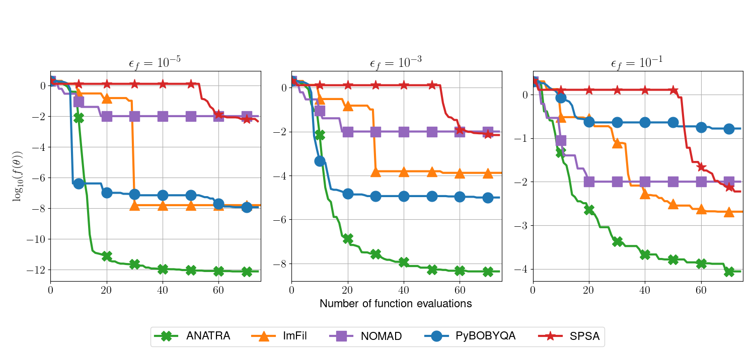
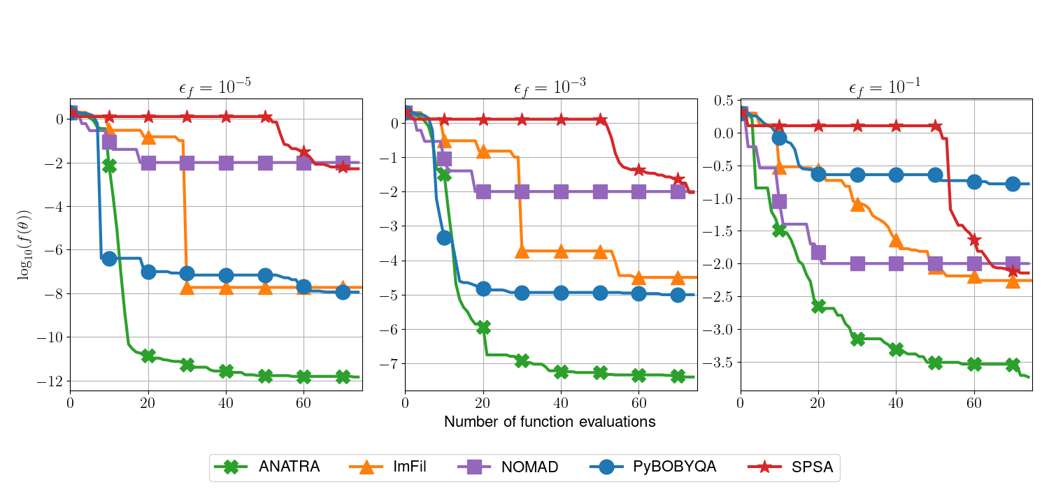
Figure 1: Results for $d=2$-dimensional quadratic problems eq. 33. Top row corresponds to uniform noise; bottom row corresponds to Gaussian noise. Throughout all of these plots, the solid lines correspond to the median ground truth objective value over 30 runs of the best point evaluated by the solver.

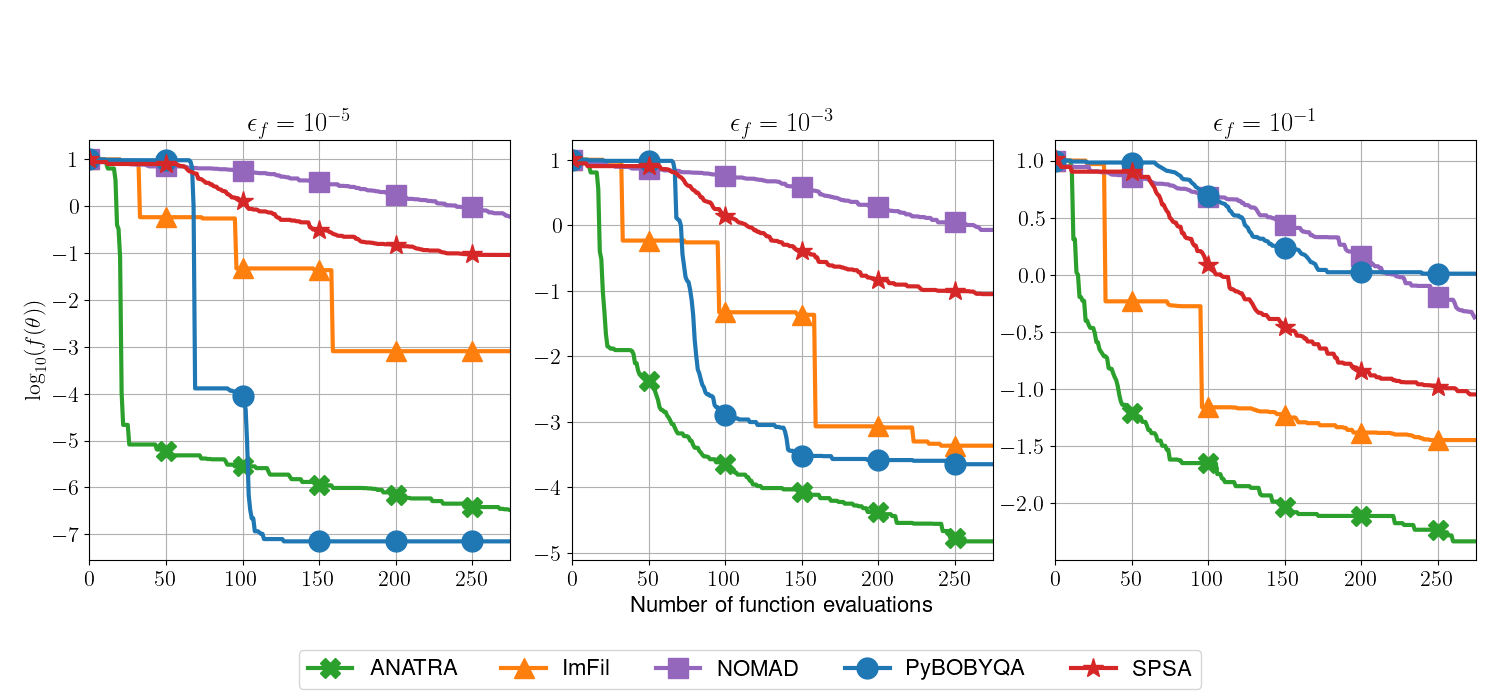
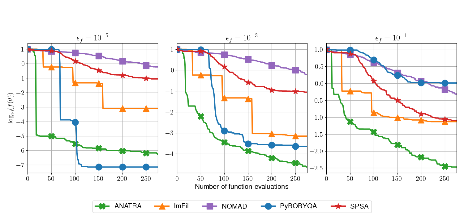
Figure 2: Same as Figure 1 but with $d=10$-dimensional quadratic functions.

A second synthetic problem that we find important for comparing derivative-free optimization methods is the standard benchmark 2-dimensional Rosenbrock function perturbed by additive noise. That is,

$$\tilde{f}(\theta,\xi)=100(\theta_{2}-\theta_{1}^{2})^{2}+(1-\theta_{1})^{2}+\xi.$$ (34)

The Rosenbrock function is especially good for testing the efficacy of model-based derivative-free methods because the Rosenbrock function is a quartic polynomial, meaning that a quadratic interpolation model will generally never be a perfect model. Moreover, the Rosenbrock function is highly nonlinear but interpretably so; any descent-seeking trajectory must turn around a curved valley, the base of which is defined by the curve $\theta_{2}=\theta_{1}^{2}$. However, even as a pathologically nonlinear and nonconvex function, the 2-dimensional Rosenbrock has exactly one local (global) minimum, making benchmarking in terms of function values straightforward.

Results comparing the median performance over 30 trials of the five solvers are displayed in Figure 3. In these runs we used the starting point of the origin, which is conveniently on the curve $\theta_{2}=\theta_{1}^{2}$; that is, this test is designed not to test an algorithm’s ability to find the bottom of the valley but instead to test an algorithm’s ability to follow the nonlinear valley to the global minimum. We note a few behaviors that did not appear in the test with the simple quadratic functions. First, one may note that SPSA does not seem to start from the same starting point as the other solvers; the reason that because of the finite differencing scheme innate to SPSA, the initial point is never actually evaluated. Moreover, because the gradient is relatively small near $\theta_{2}=\theta_{1}^{2}$ but relatively large farther away from the same curve, the gradient estimates obtained from the randomized two-point difference scheme employed by SPSA lead to a trajectory that tends to stay near the valley but never gets too close to the bottom until/unless a very small step size is employed. Of the remaining solvers, it is notable that a relative preference for NOMAD versus ImFil seems to have switched for this problem. A potential explanation for this may lie in the fact that ImFil uses a fairly rigid (coordinate-aligned) finite difference gradient estimator; this stencil centered near any point on $\theta_{2}=\theta_{1}^{2}$ will not overlap well with the valley of descent. This will trigger multiple stencil failures until the stencil size is quite small, at which point finding descent is difficult in the presence of noisy evaluations. NOMAD, on the other hand, generates polling directions less rigidly on the mesh and is more likely to identify an improving point. Of particular interest to this paper, ANATRA and PyBOBYQA perform similarly on the lowest level of noise ($\epsilon_{f}=10^{-5}$), but the preference for using ANATRA becomes increasingly clear as the noise increases.

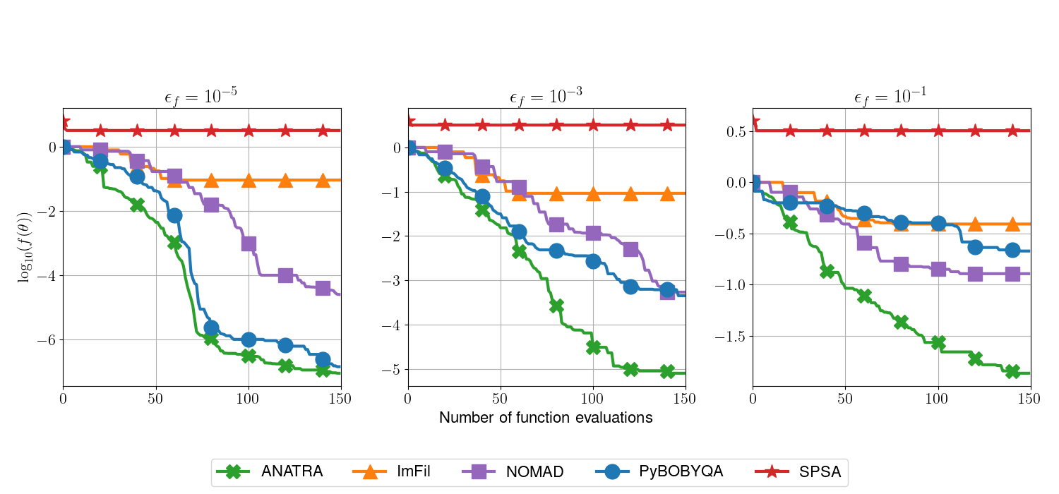
Figure 3: Comparing solvers on eq. 34. Top plots correspond to uniform noise; bottom plots correspond to Gaussian noise.

5.4 Tests on VQA Problems

The synthetic tests of the preceding section were designed to establish why we believe a noise-aware model-based method like ANATRA is a good choice for noise-perturbed smooth optimization. To further this claim, we now perform tests on standard QAOA benchmarks to demonstrate the performance of our solver on simulations of real problems, which is the original motivation for our work. We simulate QAOA MaxCut circuits in Qiskit [49] with a depth of five, resulting in a set of (ten) parameters. Of course, to mirror the real-world, we no longer assume that we know $\epsilon_{f}$ as an input to ANATRA. Instead, when we compute the sample average of the MaxCut objective values suggested by the quantum device, we additionally compute the standard error; we use the standard error as $\tilde{\epsilon}_{f}$. In our tests we vary the shot counts per function evaluation to be in $\{50,100,500,1000\}$.

We experiment with the MaxCut problem both on a toy graph with MaxCut value of 6 and on the Chvátal graph, a standard benchmark that has a MaxCut value of 20.

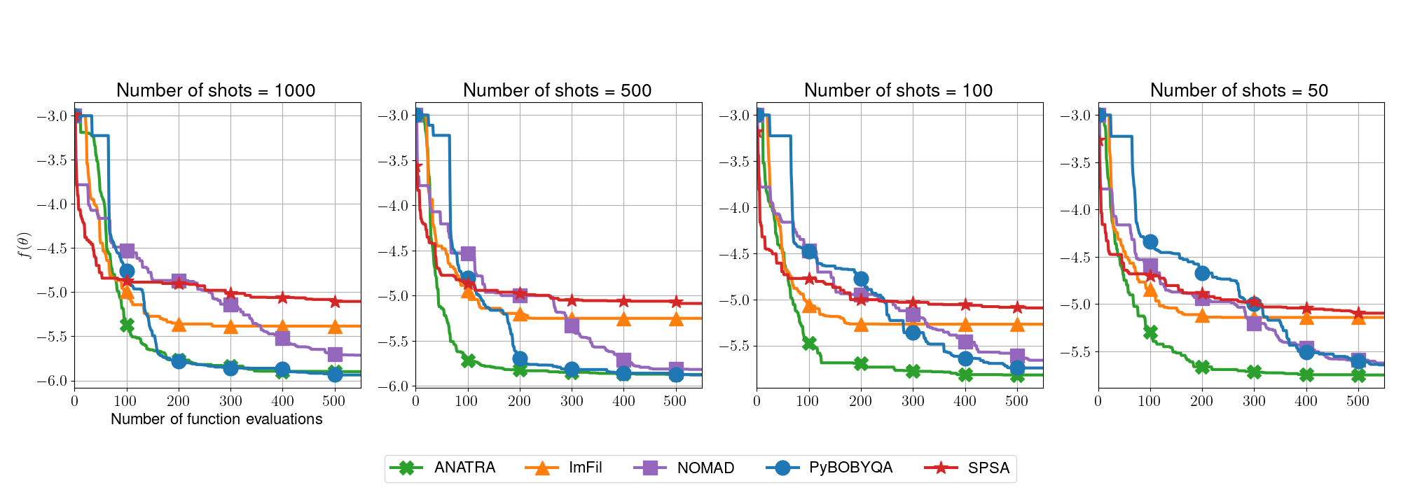
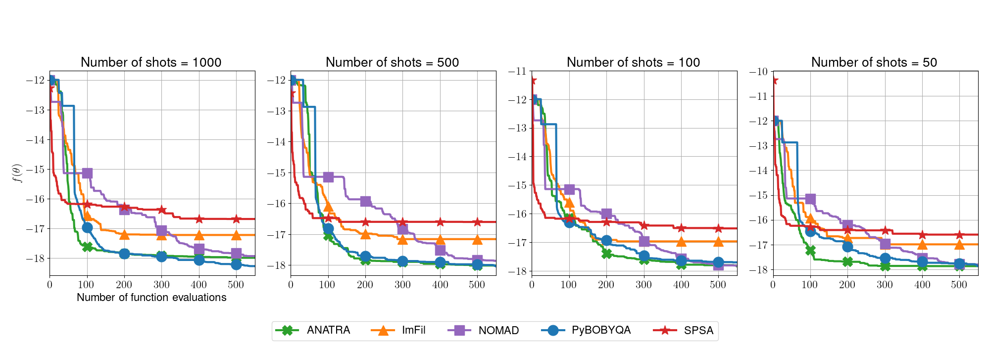
Figure 4: Comparing solvers on QAOA MaxCut problems. Top plots correspond to the toy graph, and bottom plots correspond to the Chvátal graph.

The results in Figure 4 mirror most of our expectations that came from the synthetic tests. In less noisy settings (when the shot count is 1000 shots per evaluation), there is little distinction, but perhaps a slight preference, for using PyBOBYQA over ANATRA. However, as the noise increases (the shot count decreases), we see an increasingly clear preference for employing ANATRA, both in terms of final median solution quality and in terms of efficiency to reach said median solution quality.

6 Discussion

We have presented, analyzed, and tested a noise-aware model-based trust-region algorithm to solve noisy derivative-free optimization problems, a problem class that can encompass VQA. In our theory, function evaluations are assumed to be obtained from a zeroth-order oracle with deterministically bounded noise or subexponential noise. Our proposed algorithm was based on an established noise-aware trust-region method but employed algorithmic devices to carefully maintain poisedness of interpolation points. In addition, unlike most classical model-based trust-region methods, our method decoupled the trust-region radius from the sampling radius. These two considerations were made in order to guarantee conditions concerning first-order oracles, required by the theory of the original noise-aware trust-region method, were satisfied. Building on previous results, we proved that with high probability our method exhibits a worst-case $\mathcal{O}(\epsilon^{-2})$ convergence rate to an $\epsilon$-neighborhood of a local minima provided $\epsilon$ is greater than a function of the noise level $\epsilon_{f}$. Numerical experiments demonstrate that our proposed algorithm outperforms alternative solvers, particularly in highly noisy regimes, such as when shot counts on a quantum device are low.

The work in this manuscript leaves open several avenues for future development. As mentioned, the techniques proposed in Powell [37] could alleviate the considerable per-iteration linear algebra overhead incurred by ANATRA. Negotiating between the theory and practice of these model update procedures involves nontrivial research effort. We are also interested in extending ANATRA with adaptive sampling techniques appropriate for stochastic optimization, such as those employed in ASTRO-DF [28]. While the assumptions made in Definition 1 did not require oracles to be an unbiased estimator of a ground truth function, there is a significant stochastic component to each noisy function evaluation done on a quantum computer. As long as the hardware error does not dominate the stochastic error, stochastic optimization (and hence adaptive sampling) may be appropriate. Opportunities exist for developing techniques to distinguish between stochastic and hardware noise, so that adaptive sampling may be effectively and judiciously performed in the VQA setting. The application of ANATRA to other noise settings is also of interest. For example, Definition 1 established a global property for oracles in the sense that $\epsilon_{f}$ was a constant applicable to all of $\mathcal{R}^{d}$. However, as can be seen in Algorithm 3 of Algorithm 3, ANATRA was designed assuming $\epsilon_{f}$ is in fact a local constant, intended to be relevant only on a trust region in each iteration. In problem settings where noise is known to be nonconstant with respect to problem parameters, such as many VQA settings (see, e.g., Zhang et al. [50] and references therein), a potential extension of ANATRA might attempt to model nonconstant noise. This can be done, for instance, by constructing interpolation/regression models of $\epsilon_{f}$ and employing the resulting noise model not only to perform Algorithm 3 but also to modify routines for selecting $\mathcal{X}$ to decrease the error of noisy model gradients.

Appendix A Algorithm for generating affinely independent points

Here we present an algorithm that is used in Algorithm 3 of Algorithm 3. This algorithm is based on [35][Algorithm 4.1]. Algorithm 4 begins by computing the set of displacements of each point in $\mathcal{X}$ from the center point, $x^{0}=\theta_{k}$, and initializes an empty set of points $\mathcal{Y}$ and a trivial subspace $Z=\mathcal{R}^{d}$. One displacement at a time, the algorithm checks whether the projection onto $Z$ (denoted $\textbf{Proj}_{Z}$) of a scaled displacement is sufficiently bounded away from zero (that is, the method checks whether the displacement is not sufficiently close to being orthogonal to $Z$). If the projection is sufficiently large, then the displacement is added to the set $\mathcal{Y}$, and the subspace $Z$ is updated to be the null space to the span of the displacement vectors in $\mathcal{Y}$, denoted $\textbf{Null}(\textbf{Span}(\mathcal{Y}))$. After looping over all $p$ points, Algorithm 4 returns the union of $x^{0}$, the $x^{i}\in\mathcal{X}$ such that $d^{i}$ was added to $\mathcal{Y}$, and the set $\{x^{0}+\textbf{Basis}(Z)\}$, where $\textbf{Basis}(Z)$ denotes an arbitrary basis for $Z$. In our implementation, and as intended in [35], all of these projections and null space operations are handled via a QR factorization with insertions, and the final basis for $Z$ is taken as appropriate columns of the orthogonal $Q$ factor. When we call Algorithm 4 from Algorithm 3, the choice of $\mathcal{X},c_{s},$ and $\Delta_{k}$ is transparent. We set $\tau=10^{-5}$.

Input: Set of points $\mathcal{X}=\{x^{0},x^{1},\dots,x^{p}\}\subset\mathcal{R}^{d}$, constants $c_{s}\geq 1$, $\tau\in(0,1/c_{s}]$, trust region $\Delta_{k}$.

1 Set $\mathcal{D}:=\{d^{i}=x^{i}-x^{0}:i=1,\dots,p\}$.

2 Initialize $\mathcal{Y}=\emptyset$, $Z=\mathcal{R}^{d}$.

3 for $i=1,\dots,p$ do

4       if $\left|\textbf{Proj}_{Z}\left(\frac{1}{c_{s}\Delta_{k}}d^{i}\right)\right|\geq\tau$ then

5             $\mathcal{Y}\leftarrow\mathcal{Y}\cup\{d^{i}\}$

6             $Z\leftarrow\textbf{Null}(\textbf{Span}(\mathcal{Y}))$

7            

8      

$\mathcal{X}\leftarrow\{x^{0}\}\cup\{x^{i}:d^{i}\in\mathcal{Y}\}\cup\{x^{0}+\textbf{Basis}(Z)\}$.

Algorithm 4 Generating a set of affinely independent points

References

- Cerezo et al. [2021] M. Cerezo, Andrew Arrasmith, Ryan Babbush, Simon C. Benjamin, Suguru Endo, Keisuke Fujii, Jarrod R. McClean, Kosuke Mitarai, Xiao Yuan, Lukasz Cincio, and Patrick J. Coles. Variational quantum algorithms. Nature Reviews Physics, 3(9):625–644, August 2021. doi:10.1038/s42254-021-00348-9.
- McClean et al. [2016] Jarrod R McClean, Jonathan Romero, Ryan Babbush, and Alán Aspuru-Guzik. The theory of variational hybrid quantum-classical algorithms. New Journal of Physics, 18(2):023023, February 2016. doi:10.1088/1367-2630/18/2/023023.
- Farhi et al. [2014] Edward Farhi, Jeffrey Goldstone, and Sam Gutmann. A quantum approximate optimization algorithm. arXiv:1411.4028, 2014. doi:10.48550/arXiv.1411.4028.
- Wang et al. [2018] Zhihui Wang, Stuart Hadfield, Zhang Jiang, and Eleanor G. Rieffel. Quantum approximate optimization algorithm for MaxCut: A fermionic view. Physical Review A, 97(2), February 2018. doi:10.1103/physreva.97.022304.
- Shaydulin et al. [2023a] Ruslan Shaydulin, Phillip C. Lotshaw, Jeffrey Larson, James Ostrowski, and Travis S. Humble. Parameter transfer for quantum approximate optimization of weighted MaxCut. ACM Transactions on Quantum Computing, 4(3):1–15, 2023a. doi:10.1145/3584706.
- Shaydulin et al. [2023b] Ruslan Shaydulin, Changhao Li, Shouvanik Chakrabarti, Dylan Herman, Niraj Kumar, Jeffrey Larson, Danylo Lykov, Pierre Minssen, Yue Sun, Yuri Alexeev, Matthew DeCross, Joan M. Dreiling, John P. Gaebler, Thomas M. Gatterman, Justin A. Gerber, Kevin Gilmore, Dan Gresh, Nathan Hewitt, Chandler V. Horst, Shaohan Hu, Jacob Johansen, Mitchell Matheny, Tanner Mengle, Michael Mills, Steven A. Moses, Brian Neyenhuis, Peter Siegfried, Romina Yalovetzky, and Marco Pistoia. Evidence of scaling advantage for the quantum approximate optimization algorithm on a classically intractable problem. arXiv:2308.02342, 2023b. doi:10.48550/arXiv.2308.02342.
- Kandala et al. [2017] Abhinav Kandala, Antonio Mezzacapo, Kristan Temme, Maika Takita, Markus Brink, Jerry M. Chow, and Jay M. Gambetta. Hardware-efficient variational quantum eigensolver for small molecules and quantum magnets. Nature, 549(7671):242–246, September 2017. doi:10.1038/nature23879.
- Grimsley et al. [2019] Harper R. Grimsley, Sophia E. Economou, Edwin Barnes, and Nicholas J. Mayhall. An adaptive variational algorithm for exact molecular simulations on a quantum computer. Nature Communications, 10(1), July 2019. doi:10.1038/s41467-019-10988-2.
- McCaskey et al. [2019] Alexander J McCaskey, Zachary P Parks, Jacek Jakowski, Shirley V Moore, Titus D Morris, Travis S Humble, and Raphael C Pooser. Quantum chemistry as a benchmark for near-term quantum computers. npj Quantum Information, 5(1):99, 2019. doi:10.1038/s41534-019-0209-0.
- Yeter-Aydeniz et al. [2021] Kübra Yeter-Aydeniz, Bryan T Gard, Jacek Jakowski, Swarnadeep Majumder, George S Barron, George Siopsis, Travis S Humble, and Raphael C Pooser. Benchmarking quantum chemistry computations with variational, imaginary time evolution, and Krylov space solver algorithms. Advanced Quantum Technologies, 4(7):2100012, 2021. doi:10.1002/qute.202100012.
- Bauer et al. [2020] Bela Bauer, Sergey Bravyi, Mario Motta, and Garnet Kin-Lic Chan. Quantum algorithms for quantum chemistry and quantum materials science. Chemical Reviews, 120(22):12685–12717, October 2020. doi:10.1021/acs.chemrev.9b00829.
- Schuld et al. [2019] Maria Schuld, Ville Bergholm, Christian Gogolin, Josh Izaac, and Nathan Killoran. Evaluating analytic gradients on quantum hardware. Physical Review A, 99(3), March 2019. doi:10.1103/physreva.99.032331.
- Menickelly et al. [2023a] Matt Menickelly, Yunsoo Ha, and Matthew Otten. Latency considerations for stochastic optimizers in variational quantum algorithms. Quantum, 7:949, 2023a. doi:10.22331/q-2023-03-16-949.
- Menickelly et al. [2023b] Matt Menickelly, Stefan M Wild, and Miaolan Xie. A stochastic quasi-Newton method in the absence of common random numbers. arXiv:2302.09128, 2023b. doi:10.48550/arXiv.2302.09128.
- Kübler et al. [2020] Jonas M Kübler, Andrew Arrasmith, Lukasz Cincio, and Patrick J Coles. An adaptive optimizer for measurement-frugal variational algorithms. Quantum, 4:263, 2020. doi:10.22331/q-2020-05-11-263.
- Arrasmith et al. [2020] Andrew Arrasmith, Lukasz Cincio, Rolando D Somma, and Patrick J Coles. Operator sampling for shot-frugal optimization in variational algorithms. arXiv:2004.06252, 2020. doi:10.48550/arXiv.2004.06252.
- Gu et al. [2021] Andi Gu, Angus Lowe, Pavel A Dub, Patrick J Coles, and Andrew Arrasmith. Adaptive shot allocation for fast convergence in variational quantum algorithms. arXiv:2108.10434, 2021. doi:10.48550/arXiv.2108.10434.
- Ito [2023] Kosuke Ito. Latency-aware adaptive shot allocation for run-time efficient variational quantum algorithms. arXiv:2302.04422, 2023. doi:10.48550/arXiv.2302.04422.
- Shaydulin et al. [2019] Ruslan Shaydulin, Ilya Safro, and Jeffrey Larson. Multistart methods for quantum approximate optimization. In Proceedings of the IEEE High Performance Extreme Computing Conference, 2019. doi:10.1109/hpec.2019.8916288.
- Larson et al. [2019] Jeffrey Larson, Matt Menickelly, and Stefan M. Wild. Derivative-free optimization methods. Acta Numerica, 28:287–404, 2019. doi:10.1017/s0962492919000060.
- Lavrijsen et al. [2020] Wim Lavrijsen, Ana Tudor, Juliane Müller, Costin Iancu, and Wibe De Jong. Classical optimizers for noisy intermediate-scale quantum devices. In IEEE International Conference on Quantum Computing and Engineering, pages 267–277. IEEE, 2020. doi:10.1109/QCE49297.2020.00041.
- Conn et al. [2009] Andrew R. Conn, Katya Scheinberg, and Luís N. Vicente. Introduction to Derivative-Free Optimization. SIAM, 2009. doi:10.1137/1.9780898718768.
- Powell [2009] Michael J. D. Powell. The BOBYQA algorithm for bound constrained optimization without derivatives. Technical Report DAMTP 2009/NA06, University of Cambridge, 2009. URL http://www.damtp.cam.ac.uk/user/na/NA_papers/NA2009_06.pdf.
- Moré and Wild [2011] Jorge J Moré and Stefan M Wild. Estimating computational noise. SIAM Journal on Scientific Computing, 33(3):1292–1314, 2011. doi:10.1137/100786125.
- Chen et al. [2018] Ruobing Chen, Matt Menickelly, and Katya Scheinberg. Stochastic optimization using a trust-region method and random models. Mathematical Programming, 169(2):447–487, 2018. doi:10.1007/s10107-017-1141-8.
- Blanchet et al. [2019] Jose Blanchet, Coralia Cartis, Matt Menickelly, and Katya Scheinberg. Convergence rate analysis of a stochastic trust-region method via supermartingales. INFORMS Journal on Optimization, 1(2):92–119, 2019. doi:10.1287/ijoo.2019.0016.
- Larson and Billups [2016] Jeffrey Larson and Stephen C. Billups. Stochastic derivative-free optimization using a trust region framework. Computational Optimization and Applications, 64(3):619–645, 2016. doi:10.1007/s10589-016-9827-z.
- Shashaani et al. [2018] Sara Shashaani, Fatemeh S. Hashemi, and Raghu Pasupathy. ASTRO-DF: A class of adaptive sampling trust-region algorithms for derivative-free stochastic optimization. SIAM Journal on Optimization, 28(4):3145–3176, 2018. doi:10.1137/15m1042425.
- Chang et al. [2013] Kuo-Hao Chang, L. Jeff Hong, and Hong Wan. Stochastic trust-region response-surface method (STRONG)–A new response-surface framework for simulation optimization. INFORMS Journal on Computing, 25(2):230–243, May 2013. doi:10.1287/ijoc.1120.0498.
- Menhorn et al. [2022] Friedrich Menhorn, Florian Augustin, Hans-Joachim Bungartz, and Youssef M. Marzouk. A trust-region method for derivative-free nonlinear constrained stochastic optimization. arXiv:1703.04156, 2022. doi:10.48550/arXiv.1703.04156.
- Sun and Nocedal [2022] Shigeng Sun and Jorge Nocedal. A trust region method for the optimization of noisy functions. arXiv:2201.00973, 2022. doi:10.48550/arXiv.2201.00973.
- Cao et al. [2023] Liyuan Cao, Albert S. Berahas, and Katya Scheinberg. First- and second-order high probability complexity bounds for trust-region methods with noisy oracles. Mathematical Programming, July 2023. doi:10.1007/s10107-023-01999-5.
- Proctor et al. [2020] Timothy Proctor, Melissa Revelle, Erik Nielsen, Kenneth Rudinger, Daniel Lobser, Peter Maunz, Robin Blume-Kohout, and Kevin Young. Detecting and tracking drift in quantum information processors. Nature Communications, 11(1), October 2020. doi:10.1038/s41467-020-19074-4.
- Berahas et al. [2022] Albert S Berahas, Liyuan Cao, Krzysztof Choromanski, and Katya Scheinberg. A theoretical and empirical comparison of gradient approximations in derivative-free optimization. Foundations of Computational Mathematics, 22(2):507–560, 2022. doi:10.1007/s10208-021-09513-z.
- Wild [2008] Stefan M. Wild. MNH: A derivative-free optimization algorithm using minimal norm Hessians. In Tenth Copper Mountain Conference on Iterative Methods, 2008. URL http://grandmaster.colorado.edu/~copper/2008/SCWinners/Wild.pdf.
- Wild [2017] Stefan M Wild. Chapter 40: POUNDERS in TAO: Solving derivative-free nonlinear least-squares problems with POUNDERS. In Advances and trends in optimization with engineering applications, pages 529–539. SIAM, 2017. doi:10.1137/1.9781611974683.ch40.
- Powell [2003] M.J.D. Powell. Least Frobenius norm updating of quadratic models that satisfy interpolation conditions. Mathematical Programming, 100(1), November 2003. doi:10.1007/s10107-003-0490-7.
- Cartis et al. [2019] Coralia Cartis, Jan Fiala, Benjamin Marteau, and Lindon Roberts. Improving the flexibility and robustness of model-based derivative-free optimization solvers. ACM Transactions on Mathematical Software, 45(3):1–41, 2019. doi:10.1145/3338517.
- Le Digabel [2011] Sébastien Le Digabel. Algorithm 909: NOMAD: Nonlinear optimization with the MADS algorithm. ACM Transactions on Mathematical Software, 37(4):1–15, February 2011. doi:10.1145/1916461.1916468.
- Kelley [2011] C. T. Kelley. Implicit Filtering. Society for Industrial and Applied Mathematics, 2011. doi:10.1137/1.9781611971903.
- Huyer and Neumaier [2008] Waltraud Huyer and Arnold Neumaier. SNOBFIT – Stable noisy optimization by branch and fit. ACM Transactions on Mathematical Software, 35(2):1–25, July 2008. doi:10.1145/1377612.1377613.
- Gilmore and Kelley [1995] P. Gilmore and C. T. Kelley. An implicit filtering algorithm for optimization of functions with many local minima. SIAM Journal on Optimization, 5(2):269–285, May 1995. doi:10.1137/0805015.
- Audet and Dennis [2006] Charles Audet and J. E. Dennis. Mesh adaptive direct search algorithms for constrained optimization. SIAM Journal on Optimization, 17(1):188–217, January 2006. doi:10.1137/040603371.
- Audet et al. [2021] Charles Audet, Kwassi Joseph Dzahini, Michael Kokkolaras, and Sébastien Le Digabel. Stochastic mesh adaptive direct search for blackbox optimization using probabilistic estimates. Computational Optimization and Applications, 79(1):1–34, 2021. doi:10.1007/s10589-020-00249-0.
- Spall [1992] J.C. Spall. Multivariate stochastic approximation using a simultaneous perturbation gradient approximation. IEEE Transactions on Automatic Control, 37(3):332–341, March 1992. doi:10.1109/9.119632.
- Gerencsér [1997] László Gerencsér. Rate of Convergence of Moments of Spall’s SPSA Method, pages 67–75. Birkhäuser Boston, 1997. doi:10.1007/978-1-4612-1980-4_7.
- Kleinman et al. [1999] Nathan L. Kleinman, James C. Spall, and Daniel Q. Naiman. Simulation-based optimization with stochastic approximation using common random numbers. Management Science, 45(11):1570–1578, November 1999. doi:10.1287/mnsc.45.11.1570.
- IBMQ [2024] IBMQ. IBM Quantum Documentation: SPSA, 2024. Available at https://docs.quantum.ibm.com/api/qiskit/qiskit.algorithms.optimizers.SPSA accessed on Jan. 12, 2024.
- Qiskit Contributors [2023] Qiskit Contributors. Qiskit: An open-source framework for quantum computing, 2023.
- Zhang et al. [2022] Dan-Bo Zhang, Bin-Lin Chen, Zhan-Hao Yuan, and Tao Yin. Variational quantum eigensolvers by variance minimization. Chinese Physics B, 31(12):120301, 2022. doi:10.1088/1674-1056/ac8a8d.