Towards Principled Graph Transformers

Abstract

The expressive power of graph learning architectures based on the $k$-dimensional Weisfeiler–Leman ($k$-WL) hierarchy is well understood. However, such architectures often fail to deliver solid predictive performance on real-world tasks, limiting their practical impact. In contrast, global attention-based models such as graph transformers demonstrate strong performance in practice, but comparing their expressive power with the $k$-WL hierarchy remains challenging, particularly since these architectures rely on positional or structural encodings for their expressivity and predictive performance. To address this, we show that the recently proposed Edge Transformer, a global attention model operating on node pairs instead of nodes, has at least $3$-WL expressive power when provided with the right tokenization. Empirically, we demonstrate that the Edge Transformer surpasses other theoretically aligned architectures regarding predictive performance while not relying on positional or structural encodings.

1 Introduction

Graph Neural Networks (GNNs) are the de-facto standard in graph learning [Kipf and Welling, 2017, Gilmer et al., 2017, Scarselli et al., 2009, Xu et al., 2019a] but suffer from limited expressivity in distinguishing non-isomorphic graphs in terms of the $1$-dimensional Weisfeiler–Leman algorithm ($1$-WL) [Morris et al., 2019, Xu et al., 2019a]. Hence, recent works introduced higher-order GNNs, aligned with the $k$-dimensional Weisfeiler–Leman ($k$-WL) hierarchy for graph isomorphism testing [Azizian and Lelarge, 2021, Morris et al., 2019, 2020, 2022], resulting in more expressivity with an increase in $k>1$. The $k$-WL hierarchy draws from a rich history in graph theory [Babai, 1979, Babai and Kucera, 1979, Babai et al., 1980, Cai et al., 1992, Weisfeiler and Leman, 1968], offering a deep theoretical understanding of $k$-WL-aligned GNNs. While theoretically intriguing, higher-order GNNs often fail to deliver state-of-the-art performance on real-world problems, making theoretically grounded models less relevant in practice [Azizian and Lelarge, 2021, Morris et al., 2020, 2022]. In contrast, graph transformers [Glickman and Yahav, 2023, He et al., 2023, Ma et al., 2023, Rampášek et al., 2022, Ying et al., 2021] recently demonstrated state-of-the-art empirical performance. However, they draw their expressive power mostly from positional/structural encodings (PEs), making it difficult to understand these models in terms of an expressivity hierarchy such as the $k$-WL. While a few works theoretically aligned graph transformers with the $k$-WL hierarchy [Kim et al., 2021, 2022, Zhang et al., 2023], we are not aware of any works reporting empirical results for $3$-WL-equivalent graph transformers on established graph learning datasets.

In this work, we want to set the ground for graph learning architectures that are theoretically aligned with the higher-order Weisfeiler–Leman hierarchy while delivering strong empirical performance and, at the same time, demonstrate that such an alignment creates powerful synergies between transformers and graph learning. Hence, we close the gap between theoretical expressivity and real-world predictive power. To this end, we apply the Edge Transformer (ET) architecture, initially developed for systematic generalization problems [Bergen et al., 2021], to the field of graph learning. Systematic (sometimes also compositional) generalization refers to the ability of a model to generalize to complex novel concepts by combining primitive concepts observed during training and poses a challenge to even the most advanced models such as GPT-4 [Dziri et al., 2023].

Specifically, we contribute the following:

1. We propose a concrete implementation of the Edge Transformer that readily applies to various graph learning tasks.

2. We show theoretically that this Edge Transformer implementation is at least as expressive as the $3$-WL without the need for positional/structural encodings.

3. We demonstrate the benefits of aligning models with the $k$-WL hierarchy by leveraging well-known results from graph theory to develop a theoretical understanding of systematic generalization in terms of first-order logic statements.

4. We demonstrate the superior empirical performance of the resulting architecture compared to a variety of other theoretically motivated models, particularly higher-order GNNs, as well as in neural algorithmic reasoning tasks.

2 Background

We consider node-labeled graphs $G\coloneqq(V(G),E(G),\ell)$ with $n$ nodes and without self-loops, where $V(G)$ is the set of nodes, $E(G)$ is the set of edges and $\ell\colon V(G)\rightarrow\mathbb{N}$ assigns an initial color to each node. We then also construct a node feature matrix $\mathbf{F}\in\mathbb{R}^{n\times p}$ that is consistent with $\ell$, i.e., for nodes $i$ and $j$ in $V(G)$, $\mathbf{F}_{i}=\mathbf{F}_{j}$ if, and only if, $\ell(i)=\ell(j)$. Note that, for a finite subset of $\mathbb{N}$, we can always construct $\mathbf{F}$, e.g., using a one-hot encoding of the initial colors. Additionally, we also consider an edge feature tensor $\mathbf{E}\in\mathbb{R}^{n\times n\times q}$, where $\mathbf{E}_{ij}$ denotes the edge feature of the edge $(i,j)\in E(G)$. We call pairs of nodes $(i,j)\in V(G)^{2}$ node pairs or $2$-tuples. For a complete description of our notation, see Appendix B.

(a) Node pairs aggregated by triangular attention.

(b) PyTorch-like pseudo-code of triangular attention.

Figure 1: Left: Triangular attention operates over node pairs and generalizes attention to relationships between three nodes. The grid represents the $n\times n\times d$ tensor state. The illustration visualizes which representations are aggregated to update the representation of a node pair $(i,j)$. Right: Triangular attention can be implemented in parallel using Einstein summation.

3 Edge Transformers

The ET was originally designed to improve the systematic generalization abilities of machine learning models. To borrow the example from Bergen et al. [2021], a model that is presented with relations such as $\textsc{mother}(x,y)$, indicating that $y$ is the mother of $x$, could generalize to a more complex relation $\textsc{grandmother}(x,z)$, indicating that $z$ is the grandmother of $x$ if $\textsc{mother}(x,y)\wedge\textsc{mother}(y,z)$ holds true. The special form of attention used by the ET, which we will formally introduce hereafter, is designed to model such more complex relations explicitly. Indeed, leveraging our theoretical results in Section 4, in Section 5, we give a formal justification for the ET in terms of performing systematic generalization. We will now formally define the ET.

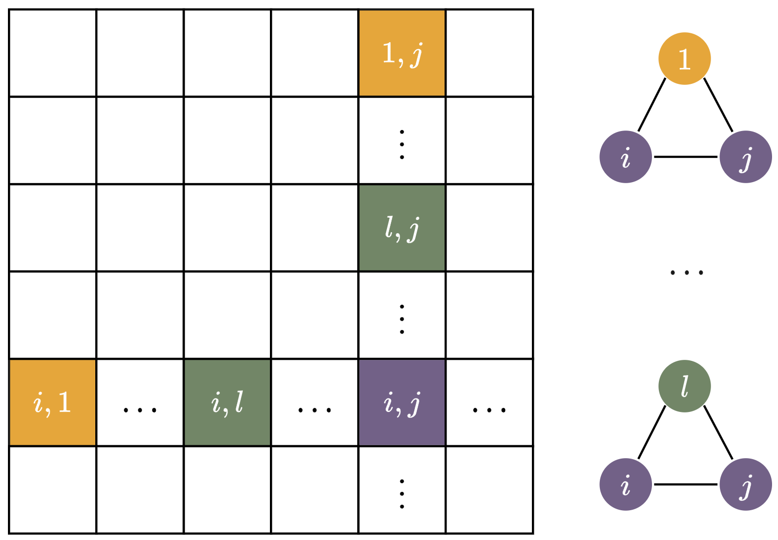
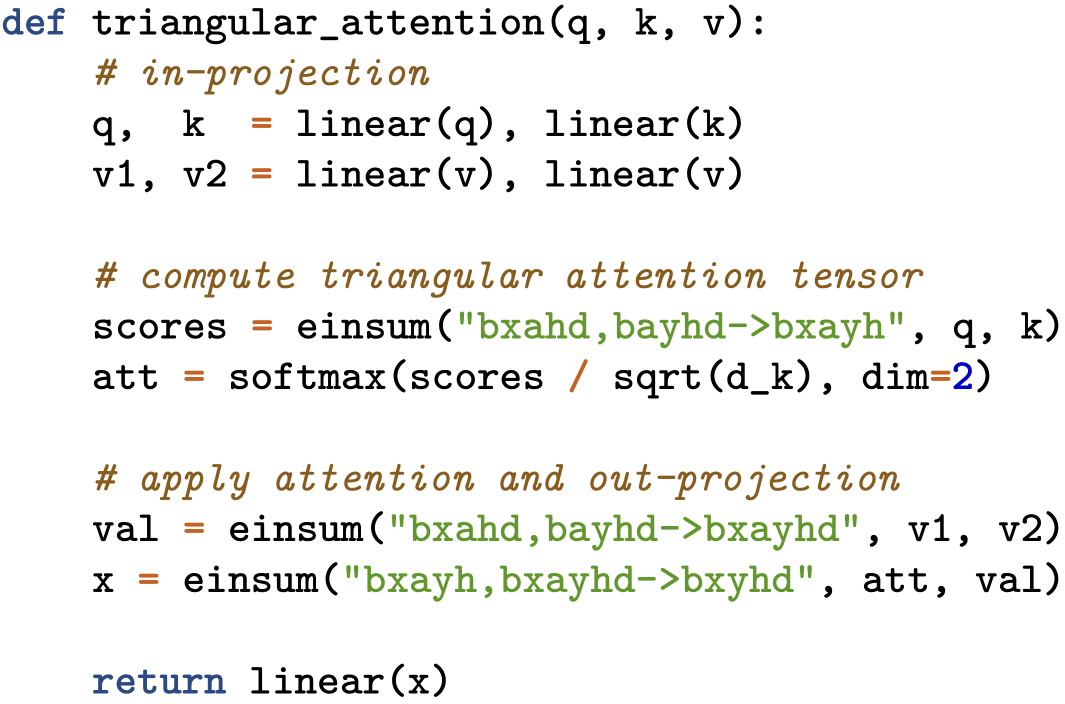
In general, the ET operates on a graph $G$ with $n$ nodes and consecutively updates a 3D tensor state $\mathbf{X}\in\mathbb{R}^{n\times n\times d}$, where $d$ is the embedding dimension and $\mathbf{X}_{ij}$ or $\mathbf{X}(\mathbf{u})$ denotes the representation of the node pair $\mathbf{u}\coloneqq(i,j)\in V(G)^{2}$. Concretely, the $t$-th ET layer computes

$$\mathbf{X}^{(t)}_{ij}\coloneqq\mathsf{FFN}\Big{(}\mathbf{X}^{(t-1)}_{ij}+\mathsf{TriangularAttn}\big{(}\mathsf{LN}\big{(}\mathbf{X}^{(t-1)}_{ij}\big{)}\big{)}\Big{)},$$

for each node pair $(i,j)$, where $\mathsf{FFN}$ is a feed-forward neural network, $\mathsf{LN}$ denotes layer normalization [Ba et al., 2016] and $\mathsf{TriangularAttn}$ is defined as

$$\mathsf{TriangularAttn}(\mathbf{X}_{ij})\coloneqq\sum_{l=1}^{n}\alpha_{ilj}\mathbf{V}_{ilj},$$ (1)

where

$$\alpha_{ilj}\coloneqq\underset{l\in[n]}{\mathsf{softmax}}\Big{(}\frac{1}{\sqrt{d}}\mathbf{X}_{il}\mathbf{W}^{Q}(\mathbf{X}_{lj}\mathbf{W}^{K})^{T}\Big{)}\in\mathbb{R}$$ (2)

is the attention score between the features of tuples $(i,l)$ and $(l,j)$. Further,

$$\mathbf{V}_{ilj}\coloneqq\mathbf{X}_{il}\mathbf{W}^{V_{1}}\odot\mathbf{X}_{lj}\mathbf{W}^{V_{2}},$$ (3)

which we call value fusion of the tuples $(i,l)$ and $(l,j)$ with $\odot$ denoting element-wise multiplication and $\mathbf{W}^{Q},\mathbf{W}^{K},\mathbf{W}^{V_{1}},\mathbf{W}^{V_{2}}\in\mathbb{R}^{d\times d}$, learnable projection matrices; see Figure 1(a) for a schematic overview of triangular attention. Moreover, Figure 1(b) illustrates that triangular attention can be computed very efficiently on modern hardware by utilizing Einstein summation [Bergen et al., 2021]. Note that similar to standard attention [Vaswani et al., 2017], triangular attention can be straightforwardly extended to multiple heads.

As we will show in Section 4, the ET owes its expressive power to the special form of triangular attention. In our implementation of the ET, we use the following tokenization, which is sufficient to obtain our theoretical result.

Tokenization

Let $G\coloneqq(V(G),E(G),\ell)$ be a graph with $n$ nodes, feature matrix $\mathbf{F}\in\mathbb{R}^{n\times p}$ and edge feature tensor $\mathbf{E}\in\mathbb{R}^{n\times n\times q}$. If no edge features are available, we randomly initialize learnable vectors $\mathbf{x}_{1},\mathbf{x}_{2}\in\mathbb{R}^{q}$ and assign $\mathbf{x}_{1}$ to $\mathbf{E}_{ij}$ if $(i,j)\in E(G)$. Further, for all $i\in V(G)$, we assign $\mathbf{x}_{2}$ to $\mathbf{E}_{ii}$. Lastly, if $(i,j)\not\in E(G)$ and $i\neq j$, we set $\mathbf{E}_{ij}=\mathbf{0}$. We then construct a 3D tensor of input tokens $\mathbf{X}\in\mathbb{R}^{n\times n\times d}$, such that for node pair $(i,j)\in V(G)^{2}$,

$$\mathbf{X}_{ij}\coloneqq\phi\Big{(}\begin{bmatrix}\mathbf{E}_{ij}&\mathbf{F}_{i}&\mathbf{F}_{j}\end{bmatrix}\Big{)}\in\mathbb{R}^{d},$$ (4)

where $\phi\colon\mathbb{R}^{2p+q}\rightarrow\mathbb{R}^{d}$ is a neural network. Extending Bergen et al. [2021], our tokenization additionally considers node features, making it more appropriate for the graph learning setting.

Efficiency

The triangular attention above imposes a $\mathcal{O}(n^{3})$ runtime and memory complexity, which is significantly more efficient than other transformers with $3$-WL expressive power, such as Kim et al. [2021] and Kim et al. [2022] with a runtime of $\mathcal{O}(n^{6})$. Nonetheless, the ET is still significantly less efficient than most graph transformers, with a runtime of $\mathcal{O}(n^{2})$ [Ying et al., 2021, Rampášek et al., 2022, Ma et al., 2023]. Thus, the ET is currently only applicable to small graphs. While certainly promising in light of the strong empirical results we demonstrate in Section 7, scaling the ET to larger graphs is out of scope for the present work.

Positional/structural encodings

Additionally, GNNs and graph transformers often benefit empirically from added positional/structural encodings [Dwivedi et al., 2022, Ma et al., 2023, Rampášek et al., 2022]. We can easily add PEs to the above tokens with the ET. Specifically, we can encode any PEs for node $i\in V(G)$ as an edge feature in $\mathbf{E}_{ii}$ and any PEs between a node pair $(i,j)\in V(G)^{2}$ as an edge feature in $\mathbf{E}_{ij}$. Note that typically, PEs between pairs of nodes are incorporated during the attention computation of graph transformers [Ma et al., 2023, Ying et al., 2021]. However, in Section 7, we demonstrate that simply adding these PEs to our tokens is also viable for improving the empirical results of the ET.

Readout

Since the Edge Transformer already builds representations on node pairs, making predictions for node pair- or edge-level tasks is straightforward. Specifically, let $L$ denote the number of Edge Transformer layers. Then, for a node pair $(i,j)\in V(G)^{2}$, we simply readout $\mathbf{X}^{(L)}_{ij}$, where on the edge-level we restrict ourselves to the case where $(i,j)\in E(G)$. In what follows, we propose a pooling method from node pairs to nodes, which allows us to also make predictions for node- and graph-level tasks. For each node $i\in V(G)$, we compute

$$\mathsf{Readout}(i)\coloneqq\sum_{j\in[n]}\rho_{1}(\mathbf{X}^{(L)}_{ij})+\rho_{2}(\mathbf{X}^{(L)}_{ji}),$$

where $\rho_{1},\rho_{2}$ are neural networks. We apply $\rho_{1}$ to node pairs where node $i$ is at the first position and $\rho_{2}$ to node pairs where node $i$ is at the second position. We found that making such a distinction has positive impacts on empirical performance. Then, for graph-level predictions, we first compute node-level readout as above and then use common graph-level pooling functions such as sum and mean [Xu et al., 2019a] or set2seq [Vinyals et al., 2016] on the resulting node representations.

With tokenization and readout as defined above, the ET can now be used on many graph learning problems, encoding both node and edge features and making predictions for node pair-, edge-, node-, and graph-level tasks. We refer to a concrete set of parameters of the ET, including tokenization and positional/structural encodings, as a parameterization. We now move on to our theoretical result, showing that the ET has an expressive power of at least the $3$-WL.

4 The Expressivity of Edge Transformers

Here, we relate the ET to the folklore Weisfeiler–Leman ($k$-FWL) hierarchy, a variant of the $k$-WL hierarchy for which we know that for $k>2$, $(k-1)$-FWL is as expressive as $k$-WL [Grohe, 2021]. Specifically, we show that the ET can simulate the $2$-FWL, resulting in $3$-WL expressive power. To this end, we briefly introduce the $2$-FWL and then show our result. For detailed background on the $k$-WL and $k$-FWL hierarchy, see Appendix B.

Folklore Weisfeiler–Leman

Let $G\coloneqq(V(G),E(G),\ell)$ be a node-labeled graph. The $2$-FWL colors the tuples from $V(G)^{2}$, similar to the way the $1$-WL colors nodes [Morris et al., 2019]. In each iteration, $t\geq 0$, the algorithm computes a coloring $C^{2,\text{F}}_{t}\colon V(G)^{2}\to\mathbb{N}$ and we write $C^{2,\text{F}}_{t}(i,j)$ or $C^{2,\text{F}}_{t}(\mathbf{u})$ to denote the color of tuple $\mathbf{u}\coloneqq(i,j)\in V(G)^{2}$ at iteration $t$. For $t=0$, we assign colors to distinguish pairs $(i,j)$ in $V(G)^{2}$ based on the initial colors $\ell(i),\ell(j)$ of their nodes and whether $(i,j)\in E(G)$. For a formal definition of the initial node pair colors, see Appendix B. Then, for each iteration, $t>0$, the coloring $C^{2,\text{F}}_{t}$ is defined as

$$C^{2,\text{F}}_{t}(i,j)\coloneqq\mathsf{RELABEL}\big{(}C^{2,\text{F}}_{t-1}(i,j),\,M_{t-1}(i,j)\big{)},$$

where $\mathsf{RELABEL}$ injectively maps the above pair to a unique natural number that has not been used in previous iterations and

$$M_{t-1}(i,j)\coloneqq\{\!\!\{\big{(}C^{2,\text{F}}_{t-1}(i,l),\,C^{2,\text{F}}_{t-1}(l,j)\big{)}\mid l\in V(G)\}\!\!\}.$$

We show that the ET can simulate the $2$-FWL.

Theorem 1.

Let $G=(V(G),E(G),\ell)$ be a node-labeled graph with $n$ nodes and $\mathbf{F}\in\mathbb{R}^{n\times p}$ be a node feature matrix consistent with $\ell$. Then for all $t\geq 0$, there exists a parametrization of the ET such that

$$C^{2,\text{F}}_{t}(\mathbf{u})=C^{2,\text{F}}_{t}(\mathbf{v})\Longleftrightarrow\mathbf{X}^{(t)}(\mathbf{u})=\mathbf{X}^{(t)}(\mathbf{v}),$$

for all pairs of $2$-tuples $\mathbf{u}$ and $\mathbf{v}\in V(G)^{2}$.

In the following, we provide some intuition of how the ET can simulate the $2$-FWL. Given a tuple $(i,j)\in V(G)^{2}$, we encode its color at iteration $t$ with $\mathbf{X}^{(t)}_{ij}$. Further, to represent the multiset

$$\{\!\!\{\big{(}C^{2,\text{F}}_{t-1}(i,l),\,C^{2,\text{F}}_{t-1}(l,j)\big{)}\mid l\in V(G)\}\!\!\},$$

we show that it is possible to encode the pair of colors

$$\big{(}C^{2,\text{F}}_{t-1}(i,l),\,C^{2,\text{F}}_{t-1}(l,j)\big{)}\quad\text{via}\quad\mathbf{X}^{(t-1)}_{il}\mathbf{W}^{V_{1}}\odot\mathbf{X}^{(t-1)}_{lj}\mathbf{W}^{V_{2}},$$

for node $l\in V(G)$. Finally, triangular attention in Equation 1, performs weighted sum aggregation over the $2$-tuple of colors $\big{(}C^{2,\text{F}}_{t-1}(i,l),\,C^{2,\text{F}}_{t-1}(l,j)\big{)}$ for each $l$, which we show is sufficient to represent the multiset; see Appendix C. Interestingly, our proof does not resort to positional/structural encodings. In fact, the ET draws its $3$-WL expressive power from its aggregation scheme, the triangular attention. In Section 7, we demonstrate that this also holds in practice, where the ET achieves strong performance without additional encodings. In what follows, we use the above results to derive a more principled understanding of the ET in terms of systematic generalization, for which it was originally designed. Thereby, we demonstrate that graph theoretic results can also be leveraged in other areas of machine learning, further highlighting the benefits of theoretically grounded models.

5 The Logic of Edge Transformers

After borrowing the ET from systematic generalization in the previous section, we now return the favor. Specifically, we use a well-known connection between graph isomorphism and first-order logic to obtain a theoretical justification for systematic generalization reasoning using the ET. Recalling the example around the grandmother relation composed from the more primitive mother relation in Section 3, Bergen et al. [2021] go ahead and argue that since self-attention of standard transformers is defined between pairs of nodes, learning explicit representations of grandmother is impossible and that learning such representations implicitly incurs a high burden on the learner. Conversely, the authors argue that since the Edge Transformer computes triangular attention over triplets of nodes and computes explicit representations between node pairs, the Edge Transformer can systematically generalize to relations such as grandmother. While Bergen et al. [2021] argue the above intuitively, we will now utilize the connection between first-order logic (FO-logic) and graph isomorphism established in Cai et al. [1992] to develop a theoretical understanding of systematic generalization; see Appendix B for an introduction to first-order logic over graphs. We will now briefly introduce the most important concepts in Cai et al. [1992] and then relate them to systematic generalization of the ET and similar models.

Language and configurations

Here, we consider FO-logic statements with counting quantifiers and denote with $\mathcal{C}_{k,m}$ the language of all such statements with at most $k$ variables and quantifier depth $m$. A configuration is a map between first-order variables and nodes in a graph. Concretely, configurations let us define a statement $\varphi$ in first-order logic, such as three nodes forming a triangle, without speaking about concrete nodes in a graph $G=(V(G),E(G))$. Instead, we can use a configuration to map the three variables in $\varphi$ to nodes $v,w,u\in V(G)$ and evaluate $\varphi$ to determine whether $v,w$ and $u$ form a triangle in $G$. Of particular importance to us are $k$-configurations $f$ where we map $k$ variables $x_{1},\dots,x_{k}$ in a FO-logic statement to a $k$-tuple $\mathbf{u}\in V(G)^{k}$ such that $\mathbf{u}=(f(x_{1}),\dotsc,f(x_{k}))$. This lets us now state the following result in Cai et al. [1992], relating FO-logic satisfiability to the $k$-FWL hierarchy.

Theorem 2 (Theorem 5.2 [Cai et al., 1992], informally).

Let $G\coloneqq(V(G),E(G))$ and $H\coloneqq(V(H),E(H))$ be two graphs with $n$ nodes and let $k\geq 1$. Let $f$ be a $k$-configuration mapping to tuple $\mathbf{u}\in V(G)^{k}$ and let $g$ be a $k$-configuration mapping to tuple $\mathbf{v}\in V(H)^{k}$. Then, for every $t\geq 0$,

$$C_{t}^{k,\text{F}}(\mathbf{u})=C_{t}^{k,\text{F}}(\mathbf{v}),$$

if, and only, if $\mathbf{u}$ and $\mathbf{v}$ satisfy the same sentences in $\mathcal{C}_{k+1,t}$.

Together with Theorem 1, we obtain the above results also for the embeddings of the ET for $k=2$.

Corollary 3.

Let $G\coloneqq(V(G),E(G))$ and $H\coloneqq(V(H),E(H))$ be two graphs with $n$ nodes and let $k=2$. Let $f$ be a $2$-configuration mapping to node pair $\mathbf{u}\in V(G)^{2}$ and let $g$ be a $2$-configuration mapping to node pair $\mathbf{v}\in V(H)^{k}$. Then, for every $t\geq 0$,

$$\mathbf{X}^{(t)}(\mathbf{u})=\mathbf{X}^{(t)}(\mathbf{v}),$$

if, and only, if $\mathbf{u}$ and $\mathbf{v}$ satisfy the same sentences in $\mathcal{C}_{3,t}$.

Systematic generalization

Returning to the example in Bergen et al. [2021], the above result tells us that a model with $2$-FWL expressive power and at least $t$ layers is equivalently able to evaluate sentences in $\mathcal{C}_{3,t}$, including

$$\textsc{grandmother}(x,z)=\exists y\big{(}\textsc{mother}(x,y)\wedge\textsc{mother}(y,z)\big{)},$$

i.e., the grandmother relation, and store this information encoded in some 2-tuple representation $\mathbf{X}^{(t)}(\mathbf{u})$, where $\mathbf{u}=(u,v)$ and $u$ is a grandmother of $v$. As a result, we have theoretical justification for the intuitive argument made by Bergen et al. [2021], namely that the ET can learn an explicit representation of a novel concept, in our example the grandmother relation.

However, when closely examining the language $\mathcal{C}_{3,t}$, we find that the above result allows for an even wider theoretical justification of the systematic generalization ability of the ET. Concretely, we will show that once the ET obtains a representation for a novel concept such as the grandmother relation, at some layer $t$, the ET can re-combine said concept to generalize to even more complex concepts. For example, consider the greatgrandmother relation, which we naively write as

$$\rho\equiv\exists a\exists z\exists y\exists x\big{(}\textsc{mother}(x,y)\wedge\textsc{mother}(y,z)\wedge\textsc{mother}(z,a)\big{)}.$$

At first glance, it seems as though $\rho\in\mathcal{C}_{4,1}$ but $\rho\not\in\mathcal{C}_{3,t}$ for any $t\geq 1$. However, notice that the variable $y$ serves merely as an intermediary to establish the grandmother relation. Hence, we can, without loss of generality, write the above as

$$\rho\equiv\exists z\exists y\exists x\big{(}\textsc{mother}(x,y)\wedge\textsc{mother}(y,z)\wedge\exists y\textsc{mother}(z,y)\big{)},$$

i.e., we re-quantify $y$ to now represent the great-grandmother of $x$. As a result, $\rho\in\mathcal{C}_{3,2}$ and hence the ET, as well as any other model with at least $2$-FWL expressive power, is able to generalize to the greatgrandmother relation within two layers, by iteratively re-combining existing concepts, in our example the grandmother and the mother relation. This becomes even more clear, by writing

$$\rho\equiv\exists z\exists y\exists x\big{(}\textsc{grandmother}(x,y)\wedge\textsc{mother}(y,z)\big{)},$$

where grandmother is a generalized concept obtained from the primitive concept mother. To summarize, knowing the expressive power of a model such as the ET in terms of the Weisfeiler–Leman hierarchy allows us to draw direct connections to the logical reasoning abilities of the model. Further, this theoretical connection allows an interpretation of systematic generalization as the ability of a model with the expressive power of at least the $k$-FWL to iteratively re-combine concepts from first principles (such as the mother relation) as a hierarchy of statements in $\mathcal{C}_{k+1,t}$, containing all FO-logic statements with counting quantifiers, at most $k+1$ variables and quantifier depth $t$.

6 Related work

In the following, we review related work. Many graph learning models with higher-order WL expressive power exist, notably $\delta$-$k$-GNNs [Morris et al., 2020], SpeqNets [Morris et al., 2022], $k$-IGNs [Maron et al., 2019c, b], PPGN [Maron et al., 2019a], and the more recent PPGN++ [Puny et al., 2023]. Moreover, Lipman et al. [2020] devised a low-rank attention module possessing the same power as the folklore $2$-WL and Bodnar et al. [2021] proposed CIN with an expressive power of at least $3$-WL. For an overview of Weisfeiler–Leman in graph learning, see Morris et al. [2021].

Many graph transformers exist, notably Graphormer [Ying et al., 2021] and GraphGPS [Rampášek et al., 2022]. However, state-of-the-art graph transformers typically rely on positional/structural encodings, which makes it challenging to derive a theoretical understanding of their expressive power. The Relational Transformer (RT) [Diao and Loynd, 2023] operates over both nodes and edges and, similar to the ET, builds relational representations, that is, representations on edges. Although the RT integrates edge information into self-attention and hence does not need to resort to positional/structural encodings, the RT is theoretically poorly understood, much like other graph transformers. Graph transformers with higher-order expressive power are Graphormer-GD [Zhang et al., 2023] and TokenGT [Kim et al., 2022] as well as the higher-order graph transformers in Kim et al. [2021]. However, Graphormer-GD is strictly less expressive than the $3$-WL[Zhang et al., 2023]. Further, Kim et al. [2021] and Kim et al. [2022] align transformers with $k$-IGNs and, thus, obtain the theoretical expressive power of the corresponding $k$-WL but do not empirically evaluate their transformers for $k>2$. For an overview of graph transformers, see Müller et al. [2023].

Finally, systematic generalization has recently been investigated both empirically and theoretically [Bergen et al., 2021, Dziri et al., 2023, Keysers et al., 2020, Ren et al., 2023]. In particular, Dziri et al. [2023] demonstrate that compositional generalization is lacking in state-of-the-art transformers such as GPT-4.

7 Experimental evaluation

In the following, we investigate how well the ET performs on various graph-learning tasks. We include tasks on graph-, node-, and edge-level and evaluate both in the inductive and transductive setting. Specifically, we answer the following questions.

Q1

How does the ET fare against other theoretically aligned architectures in terms of predictive performance?

Q2

How does the ET compare to state-of-the-art models?

Q3

How effectively can the ET benefit from additional positional/structural encodings?

The source code for our experiments is available at https://github.com/luis-mueller/towards-principled-gts. To foster research in principled graph transformers such as the ET we provide accessible implementations of the ET both in PyTorch and Jax.

Datasets

We evaluate the ET on graph-, node- and edge-level tasks from various domains to demonstrate its versatility.

On the graph level, we evaluate the ET on the molecular datasets Zinc (12K) [Dwivedi et al., 2023], Alchemy (12K), and QM9 in the setting of Morris et al. [2022]. Here, nodes represent atoms and edges bonds between atoms, and the task is always to predict one or more molecular properties of a given molecule. Due to their relatively small graphs, the above datasets are ideal for evaluating higher-order and other resource-hungry models.

On the node and edge level, we evaluate the ET on the CLRS benchmark for neural algorithmic reasoning [Velickovic et al., 2022]. Here, the input, output, and intermediate steps of 30 classical algorithms are translated into graph data, where nodes represent the algorithm input and edges are used to encode a partial ordering of the input. For example, when the input is a graph, nodes and edges are naturally derived from the input, but when the input is a list of elements, such as in sorting algorithms, CLRS encodes each element as a node and uses edges to indicate the input order; see Velickovic et al. [2022] for details on the construction of CLRS. The algorithms of CLRS are typically grouped into eight algorithm classes: Sorting, Searching, Divide and Conquer, Greedy, Dynamic Programming, Graphs, Strings, and Geometry. The task is then to predict the output of an algorithm given its input. This prediction is made based on an encoder-processor-decoder framework introduced by Velickovic et al. [2022], which is recursively applied to execute the algorithmic steps iteratively. We will use the ET as the processor in this framework, receiving as input the current algorithmic state in the form of node and edge features and outputting the updated node and edge features, according to the latest version of CLRS, available at https://github.com/google-deepmind/clrs. As such, the CLRS requires the ET to make both node- and edge-level predictions. Note that we evaluate in the single-task setting where we train a new set of parameters for each concrete algorithm, initially proposed in CLRS, to be able to fairly compare against graph transformers (see Baselines, below). We leave the multi-task learning proposed in Ibarz et al. [2022] for future work.

As well on the node-level but on a different domain than CLRS, we evaluate the ET on Cornell, Texas, and Wisconsin, three small-scale transductive datasets based on the WebKB database [Craven et al., 1998]. Here, nodes represent web pages crawled from Cornell, Texas, and Wisconsin university websites, respectively, and edges indicate a link from one website to another. The task is to predict whether a given web page shows a student, a project, a course, a staff, or a faculty. We base our experimental protocol on Morris et al. [2022].

Finally, we conduct empirical expressivity tests on the BREC benchmark [Wang and Zhang, 2023]. BREC contains 400 pairs of non-isomorphic graphs with up to 198 nodes, ranging from basic, $1$-WL distinguishable graphs to graphs even indistinguishable by $4$-WL. In addition, BREC comes with its own training and evaluation pipeline. Let $f\colon\mathcal{G}\rightarrow\mathbb{R}^{d}$ be the model whose expressivity we want to test, where $f$ maps from a set of graphs $\mathcal{G}$ to $\mathbb{R}^{d}$ for some $d>0$. Let $(G,H)$ be a pair of non-isomorphic graphs. During training, $f$ is trained to maximize the cosine distance between graph embeddings $f(G)$ and $f(H)$. During the evaluation, BREC decides whether $f$ can distinguish $G$ and $H$ by conducting a Hotelling’s T-square test with the null hypothesis that $f$ cannot distinguish $G$ and $H$.

Baselines

On the molecular regression and WebKB node-classification datasets, we compare the ET to an $1$-WL expressive GNN baseline such as GIN(E) [Xu et al., 2019b].

On the three molecular datasets we compare the ET to other theoretically-aligned models, most notably higher-order GNNs [Morris et al., 2020, 2022, Bodnar et al., 2021], Graphormer-GD, with strictly less expressive power than the $3$-WL [Zhang et al., 2023], and PPGN++, with strictly more expressive power than the $3$-WL [Puny et al., 2023] to study Q1. To study the impact of positional/structural encodings in Q3, we evaluate the ET both with and without relative random walk probabilities (RRWP) positional encodings, recently proposed in Ma et al. [2023]. RRWP encodings only apply to models with explicit representations over node pairs and are well-suited for the ET.

On the CLRS benchmark, we mostly compare to the Relational Transformer (RT) [Diao and Loynd, 2023] as a strong graph transformer baseline. Comparing the ET to the RT allows us to study Q2 in a different domain than molecular regression. Further, since the RT is similarly motivated as the ET in learning explicit representations of relations, we can study the potential benefits of the ET provable expressive power on the CLRS tasks. In addition, we compare the ET to DeepSet and GNN baselines in Diao and Loynd [2023] and the single-task Triplet-GMPNN in Ibarz et al. [2022].

On the WebKB node-classification datasets, we compare the ET to the higher-order SpeqNets [Morris et al., 2022] and additionally to the best GCN [Kipf and Welling, 2017] baseline presented in Müller et al. [2023] in aid of answering Q1. Note that the GCN baselines in Müller et al. [2023] have tuned hyper-parameters and employ additional positional/structural encodings.

On the BREC benchmark, we study questions Q1 and Q2 by comparing the ET to selected models presented in Wang and Zhang [2023]. First, we compare to the $\delta$-$2$-LGNN [Morris et al., 2020], a higher-order GNN with strictly more expressive power than the $1$-WL. Second, we compare to Graphormer [Ying et al., 2021], an empirically strong graph transformer. Third, we compare to PPGN [Maron et al., 2019a] with the same expressive power as the ET. We additionally include the $3$-WL results on the graphs in BREC to investigate how many $3$-WL distinguishable graphs the ET can distinguish in BREC.

Experimental setup

See Table 5 for an overview of the used hyperparameters.

Table 1: Average test results for the molecular regression datasets over 5 random seeds.

Model	Zinc (12K)	Alchemy (12K)	QM9
	MAE $\downarrow$	MAE $\downarrow$	MAE $\downarrow$
GIN(E) [Xu et al., 2019a, Puny et al., 2023, Morris et al., 2022]	0.163 ±0.03	0.180 ±0.006	0.079 ±0.003
$\delta$-2-LGNN [Morris et al., 2020]	0.306 ±0.044	0.122 ±0.003	0.029 ±0.001
$(2,1)$-SpeqNet [Morris et al., 2022]	-	0.169 ±0.005	0.078 ±0.007
$(2,2)$-SpeqNet [Morris et al., 2022]	-	0.115 ±0.001	0.029 ±0.001
$(3,1)$-SpeqNet [Morris et al., 2022]	-	0.180 ±0.011	0.068 ±0.003
CIN [Bodnar et al., 2021]	0.079 ±0.006	-	-
Graphormer-GD [Zhang et al., 2023]	0.081 ±0.009	-	-
SignNet [Lim et al., 2022]	0.084 ±0.006	0.113 ±0.002	-
BasisNet [Huang et al., 2023]	0.155 ±0.007	0.110 ±0.001	-
PPGN++ [Puny et al., 2023]	0.071 ±0.001	0.109 ±0.001	-
SPE [Huang et al., 2023]	0.069 ±0.004	0.108 ±0.001	-
ET	0.062 ±0.003	0.103 ± 0.001	0.017 ±0.000
ET+RRWP	0.060 ±0.003	0.102 ± 0.001	0.018 ±0.000

For Zinc (12K), we follow the hyperparameters in Ma et al. [2023] but reduce the number of layers to $6$ to make training faster. For Alchemy and QM9, we follow the hyperparameters reported in Morris et al. [2022] but reduce the number of layers to $5$ and $4$, respectively, to make training faster. We set the number of heads to $16$.

For the CLRS benchmark, we choose the same hyper-parameters as the RT. Also, following the RT, we train for 10K steps and report results over 20 different random seeds. To stay as close as possible to the experimental setup of our baselines, we integrate our Jax implementation of the ET as a processor into the latest version of CLRS and make no additional changes to the code base.

For the WebKB node-classification datasets, we start with the hyperparameters reported in Müller et al. [2023] and run a hyperparameter sweep over dropout $\in\{0.2,0.5\}$ and attention dropout $\in\{0.2,0.5\}$. Further, we set the hidden dimension to $256$ and only use ReLU non-linearity. For all of the above datasets, following Rampášek et al. [2022], we use a cosine learning rate scheduler with linear warm-up and gradient clip norm of $1.0$.

Finally, for BREC, we follow closely the setup used by Wang and Zhang [2023] for PPGN. We found learning on BREC to be quite sensitive to architectural choices, possibly due to the small dataset sizes. As a result, we use a linear layer for the FFN and additionally apply layer normalization onto $\mathbf{X}_{il}\mathbf{W}^{Q}$, $\mathbf{X}_{lj}\mathbf{W}^{K}$ in Equation 2 and $\mathbf{V}_{ilj}$ in Equation 3.

Computational resources

All experiments were performed on a mix of A10 and A100 NVIDIA GPUs. For each run, we used at most eight CPUs and at most 64 GB of RAM.

Table 2: Zinc (12K) leaderboard.

Model	Zinc (12K)
	MAE $\downarrow$
CRAWL [Tönshoff et al., 2023]	0.085 ±0.004
SignNet [Lim et al., 2022]	0.084 ±0.006
SUN [Frasca et al., 2022]	0.083 ±0.003
Graphormer-GD [Zhang et al., 2023]	0.081 ±0.009
CIN [Bodnar et al., 2021]	0.079 ±0.006
Graph-MLP-Mixer [He et al., 2023]	0.073 ±0.001
PPGN++ [Puny et al., 2023]	0.071 ±0.001
GraphGPS [Rampášek et al., 2022]	0.070 ±0.004
SPE [Huang et al., 2023]	0.069 ±0.004
Graph Diffuser [Glickman and Yahav, 2023]	0.068 ±0.002
Specformer [Bo et al., 2023]	0.066 ±0.003
GRIT [Ma et al., 2023]	0.059 ±0.002
ET	0.062 ±0.003
ET+RRWP	0.060 ±0.003

Table 3: Average test scores of different algorithm classes and average test score of all algorithms in CLRS over 10 seeds; see Section A.2 for test scores per algorithm and Section A.3 for details on the standard deviation. Baseline results for Deep Sets, GAT, MPNN, PGN, and RT are taken from Diao and Loynd [2023] and baseline results for Triplet-GMPNN are taken from Ibarz et al. [2022].

Model	Sorting	Searching	DC	Greedy	DP	Graphs	Strings	Geometry	All algorithms
Deep Sets	68.89%	50.99%	12.29%	77.83%	68.29%	42.09%	2.92%	65.47%	50.29%
GAT	21.25%	38.04%	15.19%	75.75%	63.88%	55.53%	1.57%	68.94 %	48.08%
MPNN	27.12%	43.94%	16.14%	89.40%	68.81%	63.30%	2.09%	83.03%	55.15%
PGN	28.93%	60.39%	51.30%	76.72%	71.13%	64.59%	1.82%	67.78%	56.57%
RT	50.01%	65.31%	66.52%	85.32%	83.20%	65.33%	32.52%	84.55%	66.18%
Triplet-GMPNN	60.37%	58.61%	76.36%	91.21%	81.99%	81.41%	49.09%	94.09%	75.98%
ET	79.90%	36.00%	63.84%	81.11%	83.49%	85.76%	59.83%	91.47%	77.59%

Table 4: Results on the BREC benchmark over a single seed. Baseline results are taken from Wang and Zhang [2023].

Model	Basic	Regular	Extension	CFI	All
$3$-WL	60	50	100	60	270
$\delta$-$2$-LGNN	60	50	100	6	216
PPGN	60	50	100	23	233
Graphormer	16	12	41	10	79
ET	60	50	100	47	258

Results and discussion

In the following, we answer questions Q1 to Q3. We highlight first, second, and third best results in each table.

We compare results on the molecular regression datasets in Table 1. The ET outperforms all baselines, even without using positional/structural encodings, answering Q1. Nonetheless, the RRWP encodings we employ on the graph-level datasets further improve the performance of the ET on two out of three datasets, positively answering Q3. Moreover, in Table 2, we compare the ET with a variety of graph learning models on Zinc (12K), demonstrating that the ET is highly competitive with state-of-the-art models, answering Q2.

In Table 3, we compare results on CLRS where the ET performs best when averaging all tasks, significantly improving over RT and Triplet-GMPNN. Additionally, the ET performs best on 4 algorithm classes and is among the top-3 in 6/8 algorithm classes. Interestingly, no single model is best on a majority of algorithm classes. These results indicate a benefit of the ETs’ expressive power on this benchmark, adding to the answer of Q2.

In Table 6 in Section A.1, we compare results on the WebKB node-classification datasets. Here, the ET performs best or second best on all three datasets. At the same time, for the ET we observe an increase in variance across the ten seeds compared to the baseline models, indicating that these datasets are too small to leverage the ET fully. Scaling the ET to larger transductive datasets, however, poses challenges to the cubic complexity of the ET, which we leave as future work.

Finally, on the BREC benchmark, we observe that the ET cannot distinguish all graphs distinguishable by the $3$-WL. At the same time, the ET distinguishes more graphs than PPGN, the other $3$-WL expressive model, providing an additional positive answer to Q1; see Table 4. Moreover, the ET distinguishes more graphs than $\delta$-2-LGNN and outperforms Graphormer by a large margin, again positively answering Q2. Overall, the positive results of the ET on BREC indicate that the ET is well able to leverage its expressive power empirically. In fact, the ET significantly improves distinguishing all $3$-WL distinguishable graphs in BREC.

8 Conclusion

Here, we established a previously unknown connection between the Edge Transformer and the $3$-WL and enabled the Edge Transformer for various graph learning tasks, including graph-, node-, and edge-level tasks in the inductive and transductive setting. We also utilized a well-known connection between graph isomorphism testing and first-order logic to derive a theoretical interpretation of systematic generalization. We demonstrated empirically that the Edge Transformer is a promising architecture for graph learning, outperforming other theoretically aligned architectures and being among the best models on Zinc (12K) and CLRS. Furthermore, the ET is a graph transformer that does not rely on positional/structural encodings for strong empirical performance. Future work could further explore the potential of the Edge Transformer in neural algorithmic reasoning and molecular learning by improving its scalability to larger graphs.

Appendix A Experimental details

Table 5: Hyperparameters of the Edge Transformer across all datasets.

Hyperparameter	Zinc(12K)	Alchemy	QM9	Cornell	Texas	Wisconsin	CLRS	BREC
Learning rate	0.001	0.001	0.001	0.0005	0.0005	0.0005	0.00025	0.0001
Weight decay	1e-5	1e-5	1e-5	1e-5	1e-5	1e-5	-	0.0001
Num. epochs	2 000	2 000	200	200	200	200	-	20
Num. steps	-	-	-	-	-	-	10 000	-
Grad. clip norm	1.0	1.0	1.0	1.0	1.0	1.0	1.0	-
Num. layers	6	5	4	2	2	2	3	5
Hidden dim.	64	64	64	256	256	256	192	32
Num. heads	8	16	16	8	8	8	12	4
Dropout	0.0	0.0	0.0	0.5	0.5	0.2	0.0	0.0
Attention dropout	0.2	0.1	0.1	0.5	0.5	0.2	0.0	0.0
Activation	GELU	GELU	GELU	ReLU	ReLU	ReLU	ReLU	-
Pooling	sum	set2set	set2set	-	-	-	-	-
Num. warm-up epochs/steps	50	50	5	10	10	10	0	0

Here, we give additional experimental details and results; see Table 5 for an overview over the selected hyper-parameters for all experiments.

A.1 WebKB test results

Here, we present test results for the WebKB node-classification datasets Cornell, Texas and Wisconsin; see Table 6.

Table 6: Average test results for the WebKB node-classification datasets over 10 random seeds. Baseline results for GCN are the best test results for each datasets in Müller et al. [36]. Results for the other baselines are taken from Morris et al. [35].

Model	Cornell	Texas	Wisconsin
	Accuracy $\uparrow$	Accuracy $\uparrow$	Accuracy $\uparrow$
GCN	56.2 ±2.6	66.8 ±2.7	69.4 ±2.7
GIN(E)	51.9 ±1.1	55.3 ±2.7	48.4 ±1.6
$(2,1)$-SpeqNet	63.9 ±1.7	66.8 ±0.9	67.7 ±2.2
$(2,2)$-SpeqNet	67.9 ±1.7	67.3 ±2.0	68.4 ±2.2
$(3,1)$-SpeqNet	61.8 ±3.3	68.3 ±1.3	60.4 ±2.8
ET	67.6 ±7.3	72.7 ±5.2	73.1 ±6.2

A.2 CLRS test scores

Here, we present detailed results for the algorithms in CLRS; see Table 9 for divide and conquer algorithms, Table 10 for dynamic programming algorithms, Table 11 for geometry algorithms, Table 13 for greedy algorithms, Table 8 for search algorithms, Table 7 for sorting algorithms, Table 14 for string algorithms.

Table 7: Detailed test scores for the ET on sorting algorithms.

Algorithm	Performance	Std. dev.
Bubble Sort	93.60%	3.87%
Heapsort	54.91%	29.04%
Insertion Sort	85.71%	20.68%
Quicksort	85.37%	8.70 %
Average	79.90%	15.57%

Table 8: Detailed test scores for the ET on search algorithms.

Algorithm	Performance	Std. dev.
Binary Search	4.82%	1.81%
Minimum	96.88%	1.74%
Quickselect	6.86%	6.98%
Average	36.00%	3.51%

Table 9: Detailed test scores for the ET on divide and conquer algorithms.

Algorithm	Performance	Std. dev.
Find Maximum Subarray Kadande	63.84%	2.46%
Average	63.84%	2.46%

Table 10: Detailed test scores for the ET on dynamic programming algorithms.

Algorithm	Performance	Std. dev.
LCS Length	88.67%	2.05%
Matrix Chain Order	90.11%	3.28%
Optimal BST	71.70%	5.46%
Average	83.49%	3.60%

Table 11: Detailed test scores for the ET on geometry algorithms.

Algorithm	Performance	Std. dev.
Graham Scan	92.23%	2.26%
Jarvis March	93.46%	2.14%
Segments Intersect	88.72%	6.90%
Average	91.47%	3.77%

Table 12: Detailed test scores for the ET on graph algorithms.

Algorithm	Performance	Std. dev.
Articulation Points	92.50%	3.56%
Bellman-Ford	89.96%	3.77%
BFS	99.77%	0.30%
Bridges	77.38%	33.33%
DAG Shortest Paths	96.97%	0.86%
DFS	74.30%	20.18%
Dijkstra	91.90%	2.99%
Floyd-Warshall	61.53%	5.34%
MST-Kruskal	84.76%	2.78%
MST-Prim	93.02%	2.41%
SCC	68.24%	3.66%
Topological Sort	98.74%	2.24%
Average	85.76%	6.79%

Table 13: Detailed test scores for the ET on greedy algorithms.

Algorithm	Performance	Std. dev.
Activity Selector	80.12%	12.34%
Task Scheduling	82.09%	0.75%
Average	81.11%	6.54%

Table 14: Detailed test scores for the ET on string algorithms.

Algorithm	Performance	Std. dev.
KMP Matcher	20.45%	16.05%
Naive String Match	99.21%	1.10%
Average	59.83%	8.60%

A.3 CLRS test standard deviation

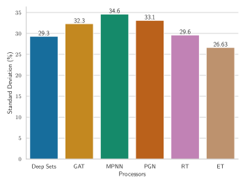
Here, we compare the standard deviation of Deep Sets, GAT, MPNN, PGN, RT and ET following the comparison in Diao and Loynd [11]; see Figure 2. We observe that the ET has the lowest overall standard deviation. Note that we omit Triplet-GMPNN [21] since we do not have access to the test results for each algorithm on each seed that are necessary to compute the overall standard deviation. Instead we compare standard deviation per algorithm class between Triplet-GMPNN and the ET in Table 15. We observe that Triplet-GMPNN and the ET have comparable standard deviation with the exception of search and string algorithms where Triplet-GMPNN has a much higher standard deviation than the ET.

Figure 2: Standard deviation of Deep Sets, GAT, MPNN, PGN, RT and ET (over all algorithms and all seeds).

Table 15: Standard deviation per algorithm class of Triplet-GMPNN (over 10 random seeds) as reported in Ibarz et al. [21] and ET (over 10 random seeds).

Algorithm class	Triplet-GMPNN	ET
Sorting	12.16%	15.57%
Searching	24.34%	3.51%
Divide and Conquer	1.34%	2.46%
Greedy	2.95%	6.54 %
Dynamic Programming	4.98%	3.60%
Graphs	6.21%	6.79%
Strings	23.49%	8.60%
Geometry	2.30%	3.77%
Average	9.72%	6.35%

Appendix B Extended preliminaries

Here, we define our notation. Let $\mathbb{N}\coloneqq\{1,2,3,\dots\}$. For $n\geq 1$, let $[n]\coloneqq\{1,\dotsc,n\}\subset\mathbb{N}$. We use $\{\!\!\{\dots\}\!\!\}$ to denote multisets, i.e., the generalization of sets allowing for multiple instances for each of its elements.

Graphs

A (node-)labeled graph $G$ is a triple $(V(G),E(G),\ell)$ with finite sets of vertices or nodes $V(G)$, edges $E(G)\subseteq\{\{u,v\}\subseteq V(G)\mid u\neq v\}$ and a (node-)label function $\ell\colon V(G)\to\mathbb{N}$. Then $\ell(v)$ is a label of $v$, for $v$ in $V(G)$. If not otherwise stated, we set $n\coloneqq|V(G)|$, and the graph is of order $n$. We also call the graph $G$ an $n$-order graph. For ease of notation, we denote the edge $\{u,v\}$ in $E(G)$ by $(u,v)$ or $(v,u)$. We define an $n$-order attributed graph as a pair $\mathbf{G}=(G,\mathbf{F})$, where $G=(V(G),E(G))$ and $\mathbf{F}$ in $\mathbb{R}^{n\times p}$ for $p>0$ is a node feature matrix. Here, we identify $V(G)$ with $[n]$, then $\mathbf{F}(v)$ in $\mathbb{R}^{1\times p}$ is the feature or attribute of the node $v\in V(G)$. Given a labeled graph $(V(G),E(G),\ell)$, a node feature matrix $\mathbf{F}$ is consistent with $\ell$ if $\ell(v)=\ell(w)$ for $v,w\in V(G)$ if, and only, if $\mathbf{F}(v)=\mathbf{F}(w)$.

Neighborhood and Isomorphism

The neighborhood of a vertex $v$ in $V(G)$ is denoted by $N(v)\coloneqq\{u\in V(G)\mid(v,u)\in E(G)\}$ and the degree of a vertex $v$ is $|N(v)|$. Two graphs $G$ and $H$ are isomorphic, and we write $G\simeq H$ if there exists a bijection $\varphi\colon V(G)\to V(H)$ preserving the adjacency relation, i.e., $(u,v)$ is in $E(G)$ if and only if $(\varphi(u),\varphi(v))$ is in $E(H)$. Then $\varphi$ is an isomorphism between $G$ and $H$. In the case of labeled graphs, we additionally require that $l(v)=l(\varphi(v))$ for $v$ in $V(G)$, and similarly for attributed graphs. Moreover, we call the equivalence classes induced by $\simeq$ isomorphism types and denote the isomorphism type of $G$ by $\tau_{G}$. We further define the atomic type $\text{atp}\colon V(G)^{k}\to\mathbb{N}$, for $k>0$, such that $\text{atp}(\mathbf{v})=\text{atp}(\mathbf{w})$ for $\mathbf{v}$ and $\mathbf{w}$ in $V(G)^{k}$ if and only if the mapping $\varphi\colon V(G)^{k}\to V(G)^{k}$ where $v_{i}\mapsto w_{i}$ induces a partial isomorphism, i.e., we have $v_{i}=v_{j}\iff w_{i}=w_{j}$ and $(v_{i},v_{j})\in E(G)\iff(\varphi(v_{i}),\varphi(v_{j}))\in E(G)$.

Matrices

Let $\mathbf{M}\in\mathbb{R}^{n\times p}$ and $\mathbf{N}\in\mathbb{R}^{n\times q}$ be two matrices then $\begin{bmatrix}\mathbf{M}&\mathbf{N}\end{bmatrix}\in\mathbb{R}^{n\times p+q}$ denotes column-wise matrix concatenation. We also write $\mathbb{R}^{d}$ for $\mathbb{R}^{1\times d}$. Further, let $\mathbf{M}\in\mathbb{R}^{p\times n}$ and $\mathbf{N}\in\mathbb{R}^{q\times n}$ be two matrices then

$$\begin{bmatrix}\mathbf{M}\\ \mathbf{N}\end{bmatrix}\in\mathbb{R}^{p+q\times n}$$

denotes row-wise matrix concatenation.

For a matrix $\mathbf{X}\in\mathbb{R}^{n\times d}$, we denote with $\mathbf{X}_{i}$ the $i$th row vector. In the case where the rows of $\mathbf{X}$ correspond to nodes in a graph $G$, we use $\mathbf{X}_{v}$ to denote the row vector corresponding to the node $v\in V(G)$.

The Weisfeiler–Leman algorithm

We describe the Weisfeiler–Leman algorithm, starting with the $1$-WL. The $1$-WL or color refinement is a well-studied heuristic for the graph isomorphism problem, originally proposed by Weisfeiler and Leman [46]. Intuitively, the algorithm determines if two graphs are non-isomorphic by iteratively coloring or labeling vertices. Formally, let $G=(V,E,\ell)$ be a labeled graph, in each iteration, $t>0$, the $1$-WL computes a vertex coloring $C^{1}_{t}\colon V(G)\to\mathbb{N}$, depending on the coloring of the neighbors. That is, in iteration $t>0$, we set

$$C^{1}_{t}(v)\coloneqq\mathsf{RELABEL}\Big{(}\!\big{(}C^{1}_{t-1}(v),\{\!\!\{C^{1}_{t-1}(u)\mid u\in N(v)\}\!\!\}\big{)}\!\Big{)},$$

for all vertices $v$ in $V(G)$, where $\mathsf{RELABEL}$ injectively maps the above pair to a unique natural number, which has not been used in previous iterations. In iteration $0$, the coloring $C^{1}_{0}\coloneqq\ell$. To test if two graphs $G$ and $H$ are non-isomorphic, we run the above algorithm in “parallel” on both graphs. If the two graphs have a different number of vertices colored $c$ in $\mathbb{N}$ at some iteration, the $1$-WL distinguishes the graphs as non-isomorphic. It is easy to see that the algorithm cannot distinguish all non-isomorphic graphs [9]. Several researchers, e.g., Babai [3], Cai et al. [9], devised a more powerful generalization of the former, today known as the $k$-dimensional Weisfeiler–Leman algorithm ($k$-WL), operating on $k$-tuples of vertices rather than single vertices.

The $k$-dimensional Weisfeiler–Leman algorithm

Due to the shortcomings of the 1-WL or color refinement in distinguishing non-isomorphic graphs, several researchers, e.g., Babai [3], Cai et al. [9], devised a more powerful generalization of the former, today known as the $k$-dimensional Weisfeiler-Leman algorithm ($k$-WL), operating on $k$-tuples of nodes rather than single nodes.

Intuitively, to surpass the limitations of the $1$-WL, the $k$-WL colors node-ordered $k$-tuples instead of a single node. More precisely, given a graph $G$, the $k$-WL colors the tuples from $V(G)^{k}$ for $k\geq 2$ instead of the nodes. By defining a neighborhood between these tuples, we can define a coloring similar to the $1$-WL. Formally, let $G$ be a graph, and let $k\geq 2$. In each iteration, $t\geq 0$, the algorithm, similarly to the $1$-WL, computes a coloring $C^{k}_{t}\colon V(G)^{k}\to\mathbb{N}$. In the first iteration, $t=0$, the tuples $\mathbf{v}$ and $\mathbf{w}$ in $V(G)^{k}$ get the same color if they have the same atomic type, i.e., $C^{k}_{0}(\mathbf{v})\coloneqq\text{atp}(\mathbf{v})$. Then, for each iteration, $t>0$, $C^{k}_{t}$ is defined by

$$C^{k}_{t}(\mathbf{v})\coloneqq\mathsf{RELABEL}\big{(}C^{k}_{t-1}(\mathbf{v}),M_{t}(\mathbf{v})\big{)},$$ (5)

with $M_{t}(\mathbf{v})$ the multiset

$$M_{t}(\mathbf{v})\coloneqq\big{(}\{\!\!\{C^{k}_{t-1}(\phi_{1}(\mathbf{v},w))\mid w\in V(G)\}\!\!\},\dots,\{\!\!\{C^{k}_{t-1}(\phi_{k}(\mathbf{v},w))\mid w\in V(G)\}\!\!\}\big{)},$$ (6)

and where

$$\phi_{j}(\mathbf{v},w)\coloneqq(v_{1},\dots,v_{j-1},w,v_{j+1},\dots,v_{k}).$$

That is, $\phi_{j}(\mathbf{v},w)$ replaces the $j$-th component of the tuple $\mathbf{v}$ with the node $w$. Hence, two tuples are adjacent or $j$-neighbors if they are different in the $j$th component (or equal, in the case of self-loops). Hence, two tuples $\mathbf{v}$ and $\mathbf{w}$ with the same color in iteration $(t-1)$ get different colors in iteration $t$ if there exists a $j$ in $[k]$ such that the number of $j$-neighbors of $\mathbf{v}$ and $\mathbf{w}$, respectively, colored with a certain color is different.

We run the $k$-WL algorithm until convergence, i.e., until for $t$ in $\mathbb{N}$

$$C^{k}_{t}(\mathbf{v})=C^{k}_{t}(\mathbf{w})\iff C^{k}_{t+1}(\mathbf{v})=C^{k}_{t+1}(\mathbf{w}),$$

for all $\mathbf{v}$ and $\mathbf{w}$ in $V(G)^{k}$ holds.

Similarly to the $1$-WL, to test whether two graphs $G$ and $H$ are non-isomorphic, we run the $k$-WL in “parallel” on both graphs. Then, if the two graphs have a different number of nodes colored $c$, for $c$ in $\mathbb{N}$, the $k$-WL distinguishes the graphs as non-isomorphic. By increasing $k$, the algorithm gets more powerful in distinguishing non-isomorphic graphs, i.e., for each $k\geq 2$, there are non-isomorphic graphs distinguished by $(k+1)$-WL but not by $k$-WL [9]. We now also define the folklore $k$-WL hierarchy.

The folklore $k$-dimensional Weisfeiler–Leman algorithm

A common and well-studied variant of the $k$-WL is the $k$-FWL, which differs from the $k$-WL only in the aggregation function. Instead of Equation 6, the “folklore” version of the $k$-WL updates $k$-tuples according to

$$M^{\text{F}}_{t}(\mathbf{v})\coloneqq\{\!\!\{(C^{k,\text{F}}_{t-1}(\phi_{1}(\mathbf{v},w)),...,C^{k,\text{F}}_{t-1}(\phi_{k}(\mathbf{v},w)))\mid w\in V(G)\}\!\!\},$$

resulting in the coloring $C^{k,\text{F}}_{t}\colon V(G)^{k}\to\mathbb{N}$, and is strictly more powerful than the $k$-WL. Specifically, for $k\geq 2$, the $k$-WL is exactly as powerful as the $(k-1)$-FWL [18].

Computing $k$-WL’s initial colors

Let $G=(V(G),E(G))$ be a graph, $k\geq 2$, and $\mathbf{u}\in V(G)^{k}$ be a $k$-tuple. Then we can present the atomic type $\text{atp}(\mathbf{v})$ by a $k\times k$ matrix $K$ over $\{1,2,3\}$. That is, the entry $K_{ij}$ is 1 if $(v_{i},v_{j})\in E(G)$, 2 if $v_{i}=v_{j}$, and 3 otherwise.

B.1 Relationship between first-order logic and Weisfeiler–Leman

We begin with a short review of Cai et al. [9]. We consider our usual node-labeled graph $G=(V(G),E(G),\ell)$ with $n$ nodes. However, we replace $\ell$ with a countable set of color relations $C_{1},\dots,C_{n}$, where for a node $v\in V(G)$,

$$C_{i}(v)\Longleftrightarrow\ell(v)=i.$$

Note that Cai et al. [9] consider the more general case where nodes can be assigned to multiple colors simultaneously. However, for our work, we assume that a node is assigned to precisely one color, and hence, the set of color relations is at most of size $n$. We can construct first-order logic statements about $G$. For example, the following sentence describes a graph with a triangle formed by two nodes with color $1$:

$$\exists x_{1}\exists x_{2}\exists x_{3}\big{(}E(x_{1},x_{2})\wedge E(x_{1},x_{3})\wedge E(x_{2},x_{3})\wedge C_{1}(x_{1})\wedge C_{1}(x_{2})\big{)}.$$

Here, $x_{1}$, $x_{2}$ and $x_{3}$ are variables which can be repeated and re-quantified at will. Statements made about $G$ and a subset of nodes in $V(G)$ are of particular importance to us. To this end, we define a $k$-configuration, a partial function $f:\{x_{1},\dots,x_{k}\}\rightarrow V(G)$ that assigns a node in $V(G)$ to one of $k$ variables. Let $\varphi$ be a first-order sentence with free variables $x_{1},\dots,x_{l}$, where $l\leq k$. Then, we write

$$G,f\models\varphi$$

if $\varphi$ is true for nodes $f(x_{1}),\dots,f(x_{l})$. Cai et al. [9] now define the language $\mathcal{C}_{k}$ of all first-order sentences with at most $k$ variables and counting quantifiers. For example, the following sentence in $\mathcal{C}_{k}$ lets us describe a graph with exactly $3$ triangles where one node has color $3$:

$$\exists!3x_{1}\exists x_{2}\exists x_{3}\big{(}E(x_{1},x_{2})\wedge E(x_{1},x_{3})\wedge E(x_{2},x_{3})\wedge C_{3}(x_{1})\big{)}.$$

Given two graphs $G$ and $H$ and respective $k$-configurations $f$ and $g$, we can now define an equivalence class $\equiv_{\mathcal{C}_{k}}$ and say that $G,f$ and $H,g$ are $\mathcal{C}_{k}$ equivalent, denoted

$$G,f\equiv_{\mathcal{C}_{k}}H,g$$

if and only if for all $\varphi\in\mathcal{C}_{k}$ with at most $k$ free variables,

$$G,f\models\varphi\Longleftrightarrow H,g\models\varphi.$$

It is important to note that configurations are used to define a concept beyond the scope of a concrete graph. Instead, a concept can be applied to a graph $G$ by defining a configuration, i.e., a mapping between concrete nodes in $G$ to abstract logical variables.

Now, Cai et al. [9] prove that, given two graphs $G$ and $H$ and respective $k$-configurations $f$ and $g$, we have that $\mathbf{u}\coloneqq(f(x_{1}),\dots,f(x_{k}))\in V(G)^{k}$ and $\mathbf{v}\coloneqq(g(x_{1}),\dots,g(x_{k}))\in V(G)^{k}$ are $k$-tuples and

$$C_{t}^{k,\text{F}}(\mathbf{u})=C_{t}^{k,\text{F}}(\mathbf{v})\Longleftrightarrow G,f\equiv_{\mathcal{C}_{k+1}}H,g,$$

for some $t\geq 0$. Using Theorem 1 we can then also say that there exists a parameterization of the ET such that

$$\mathbf{X}^{(t)}(\mathbf{u})=\mathbf{X}^{(t)}(\mathbf{v})\Longleftrightarrow G,f\equiv_{\mathcal{C}_{3}}H,g.$$

Appendix C Proof of Theorem 1

Here, we first generalize the GNN from Grohe [18] to the $2$-FWL. Higher-order GNNs with the same expressivity have been proposed in prior works by Azizian and Lelarge [1]. However, our GNNs have a special form that can be computed by the Edge Transformer.

Formally, let $S\subseteq\mathbb{N}$ be a finite subset. First, we show that multisets over $S$ can be injectively mapped to a value in the closed interval $(0,1)$, which is a variant of Lemma VIII.5 in Grohe [18]. Here, we outline a streamlined version of its proof, highlighting the key intuition behind representing multisets as $m$-ary numbers. Let $M\subseteq S$ be a multiset with multiplicities $a_{1},\dots,a_{k}$ and distinct $k$ values. We define the order of the multiset as $\sum_{i=1}^{k}a_{i}$. We can write such a multiset as a sequence $x^{(1)},\dots,x^{(l)}$ where $l$ is the order of the multiset. Note that the order of the sequence is arbitrary and that for $i\neq j$ it is possible to have $x^{(i)}=x^{(j)}$. We call such a sequence an $M$-sequence of length $l$. We now prove a slight variation of a result of Grohe [18].

Lemma 4.

For a finite $m\in\mathbb{N}$, let $M\subseteq S$ be a multiset of order $m-1$ and let $x_{i}\in S$ denote the $i$th number in a fixed but arbitrary ordering of $S$. Given a mapping $g\colon S\rightarrow(0,1)$ where

$$g(x_{i})\coloneqq m^{-i},$$

and an $M$-sequence of length $l$ given by $x^{(1)},\dots,x^{(l)}$ with positions $i^{(1)},\dots,i^{(l)}$ in $S$, the sum

$$\sum_{j\in[l]}g(x^{(j)})=\sum_{j\in[l]}m^{-i^{(j)}}$$

is unique for every unique $M$.

Proof.

By assumption, let $M\subseteq S$ denote a multiset of order $m-1$. Further, let $x^{(1)},\dots,x^{(l)}\in M$ be an $M$-sequence with $i^{(1)},\dots,i^{(l)}$ in $S$. Given our fixed ordering of the numbers in $S$ we can equivalently write $M=((a_{1},x_{1}),\dots,(a_{n},x_{n}))$, where $a_{i}$ denotes the multiplicity of $i$th number in $M$ with position $i$ from our ordering over $S$. Note that for a number $m^{-i}$ there exists a corresponding $m$-ary number written as

$$0.0\ldots\underbrace{1}_{i}\ldots$$

Then the sum,

$$\sum_{j\in[l]}g(x^{(j)}) =\sum_{j\in[l]}m^{-i^{(j)}}$$

$$=\sum_{i\in S}a_{i}m^{-i}\in(0,1)$$

and in $m$-ary representation

$$0.a_{1}\ldots a_{n}.$$

Note that $a_{i}=0$ if and only if there exists no $j$ such that $i^{(j)}=i$. Since the order of $M$ is $m-1$, it holds that $a_{i}<m$. Hence, it follows that the above sum is unique for each unique multiset $M$, implying the result. ∎

Recall that $S\subseteq\mathbb{N}$ and that we fixed an arbitrary ordering over $S$. Intuitively, we use the finiteness of $S$ to map each number therein to a fixed digit of the numbers in $(0,1)$. The finite $m$ ensures that at each digit, we have sufficient “bandwidth” to encode each $a_{i}$. Now that we have seen how to encode multisets over $S$ as numbers in $(0,1)$, we review some fundamental operations about the $m$-ary numbers defined above. We will refer to decimal numbers $m^{-i}$ as corresponding to an $m$-ary number

$$0.0\ldots\underbrace{1}_{i}\ldots,$$

where the $i$th digit after the decimal point is $1$ and all other digits are $0$, and vice versa.

To begin with, addition between decimal numbers implements counting in $m$-ary notation, i.e.,

$$m^{-i}+m^{-j}\text{ corresponds to }0.0\ldots\underbrace{1}_{i}\ldots\underbrace{1}_{j}\ldots,$$

for digit positions $i\neq j$ and

$$m^{-i}+m^{-j}\text{ corresponds to }0.0\ldots\underbrace{2}_{i=j}\ldots,$$

otherwise. We used counting in the previous result’s proof to represent a multiset’s multiplicities. Next, multiplication between decimal numbers implements shifting in $m$-ary notation, i.e.,

$$m^{-i}\cdot m^{-j}\text{ corresponds to }0.0\ldots\underbrace{1}_{i+j}\ldots.$$

Shifting further applies to general decimal numbers in $(0,1)$. Let $x\in(0,1)$ correspond to an $m$-ary number with $l$ digits,

$$0.a_{1}\ldots a_{l}.$$

Then,

$$m^{-i}\cdot x\text{ corresponds to }0.0\ldots 0\underbrace{a_{1}\ldots a_{l}}_{i+1,\dots,i+l}.$$

Before we continue, we show a small lemma stating that two non-overlapping sets of $m$-ary numbers preserve their uniqueness under addition.

Lemma 5.

Let $A$ and $B$ be two sets of $m$-ary numbers for some $m>1$. If

$$\min_{x\in A}x>\max_{y\in B}y,$$

then for any $x_{1},x_{2}\in A,y_{1},y_{2}\in B$,

$$x_{1}+y_{1}=x_{2}+y_{2}\Longleftrightarrow x_{1}=x_{2}\text{ and }y_{1}=y_{2}.$$

Proof.

The statement follows from the fact that if

$$\min_{x\in A}x>\max_{y\in B}y,$$

then numbers in $A$ and numbers in $B$ do not overlap in terms of their digit range. Specifically, there exists some $l>0$ such that we can write

$$x \coloneqq 0.x_{1}\dots x_{l}$$

$$y \coloneqq 0.\underbrace{0\dots 0}_{l}y_{1}\dots y_{k},$$

for some $k>l$ and all $x\in A$, $y\in B$. As a result,

$$x+y=0.x_{1}\dots x_{l}y_{1}\dots y_{k}.$$

Hence, $x+y$ is unique for every unique pair $(x,y)$. This completes the proof. ∎

We begin by showing the following proposition, showing that the tokenization in Equation 4 is sufficient to encode the initial node colors under $2$-FWL.

Proposition 6.

Let $G=(V(G),E(G),\ell)$ be a node-labeled graph with $n$ nodes. Then, there exists a parameterization of Equation 4 with $d=1$ such that for each $2$-tuples $\mathbf{u},\mathbf{v}\in V(G)^{2}$,

$$C^{2,\text{F}}_{0}(\mathbf{u})=C^{2,\text{F}}_{0}(\mathbf{v})\Longleftrightarrow\mathbf{X}(\mathbf{u})=\mathbf{X}(\mathbf{v}).$$

Proof.

The statement directly follows from the fact that the initial color of a tuple $\mathbf{u}\coloneqq(i,j)$ depends on the atomic type and the node labeling. In Equation 4, we encode the atomic type with $\mathbf{E}_{ij}$ and the node labels with

$$\begin{bmatrix}\mathbf{E}_{ij}&\mathbf{F}_{i}&\mathbf{F}_{j}\end{bmatrix}$$

The concatenation of both node labels and atomic type is clearly injective. Finally, since there are at most $n^{2}$ distinct initial colors of the $2$-FWL, said colors can be well represented within $\mathbb{R}$, hence there exists an injective $\phi$ in Equation 4 with $d=1$. This completes the proof. ∎

We now show that the Edge Transformer can simulate the $2$-FWL.

Theorem 7 (Theorem 1 in main paper).

Let $G=(V(G),E(G),\ell)$ be a node-labeled graph with $n$ nodes and $\mathbf{F}\in\mathbb{R}^{n\times p}$ be a node feature matrix consistent with $\ell$. Then for all $t\geq 0$, there exists a parametrization of the ET such that

$$C^{2,\text{F}}_{t}(\mathbf{v})=C^{2,\text{F}}_{t}(\mathbf{w})\Longleftrightarrow\mathbf{X}^{(t)}(\mathbf{v})=\mathbf{X}^{(t)}(\mathbf{w}),$$

for all pairs of $2$-tuples $\mathbf{v}$ and $\mathbf{w}\in V(G)^{2}$.

Proof.

We begin by stating that our domain is compact since the ET merely operates on at most $n$ possible node features in $\mathbf{F}$ and binary edge features in $\mathbf{E}$ and at each iteration there exist at most $n^{2}$ distinct $2$-FWL colors. We prove our statement by induction over iteration $t$. For the base case, we can simply invoke Proposition 6 since our input tokens are constructed according to Equation 4. Nonetheless, we show a possible initialization of the tokenization that is consistent with Equation 4 that we will use in the induction step.

From Proposition 6 we know that the color representation of a tuple can be represented in $\mathbb{R}$. We denote the color representation of a tuple $\mathbf{u}=(i,j)$ at iteration $t$ as $\mathbf{T}^{(t)}(\mathbf{u})$ and $\mathbf{T}^{(t)}_{ij}$ interchangeably. We choose a $\phi$ in Equation 4 such that for each $\mathbf{u}=(i,j)$

$$\mathbf{X}^{(0)}_{ij}=\begin{bmatrix}\mathbf{T}^{(0)}_{ij}&\Big{(}\mathbf{T}^{(0)}_{ij}\Big{)}^{n^{2}}\end{bmatrix}\in\mathbb{R}^{2},$$

where we store the tuple features, one with exponent $1$ and once with exponent $n^{2}$ and where $\mathbf{T}^{(0)}_{ij}\in\mathbb{R}$ and $\Big{(}\mathbf{T}^{(0)}_{ij}\Big{)}^{n^{2}}\in\mathbb{R}$. Concretely, we define an injective function $f_{t}:V(G)^{2}\rightarrow[n^{2}]$ that maps each $2$-tuple $\mathbf{u}$ to a number in $[n^{2}]$ unique for its $2$-FWL color $C^{2,\text{F}}_{t}(\mathbf{u})$ at iteration $t$. Note that $f_{t}$ can be injective because there can at most be $[n^{2}]$ unique numbers under the $2$-FWL. We can then choose $\phi$ in Equation 4 such that for each $(i,j)\in V(G)^{2}$,

$$\big{|}\big{|}\mathbf{T}^{(0)}_{ij}-n^{-f_{0}(i,j)}\big{|}\big{|}_{F}<\epsilon_{0},$$

for all $\epsilon_{0}>0$, by the universal function approximation theorem, which we can invoke since our domain is compact. We will use $\Big{(}\mathbf{T}^{(0)}_{ij}\Big{)}^{n^{2}}$ in the induction step; see below.

For the induction, we assume that

$$C^{2,\text{F}}_{t-1}(\mathbf{v})=C^{2,\text{F}}_{t-1}(\mathbf{w})\Longleftrightarrow\mathbf{T}^{(t-1)}(\mathbf{v})=\mathbf{T}^{(t-1)}(\mathbf{w})$$

and that

$$\big{|}\big{|}\mathbf{T}^{(t-1)}_{ij}-n^{-f_{t-1}(i,j)}\big{|}\big{|}_{F}<\epsilon_{t-1},$$

for all $\epsilon_{t-1}>0$ and $(i,j)\in V(G)^{2}$. We then want to show that there exists a parameterization of the $t$-th layer such that

$$C^{2,\text{F}}_{t}(\mathbf{v})=C^{2,\text{F}}_{t}(\mathbf{w})\Longleftrightarrow\mathbf{T}^{(t)}(\mathbf{v})=\mathbf{T}^{(t)}(\mathbf{w})$$ (7)

and that

$$\big{|}\big{|}\mathbf{T}^{(t)}_{ij}-n^{-f_{t}(i,j)}\big{|}\big{|}_{F}<\epsilon_{t},$$

for all $\epsilon_{t}>0$ and $(i,j)\in V(G)^{2}$. Clearly, if this holds for all $t$, then the proof statement follows. Thereto, we show that the ET updates the tuple representation of tuple $(j,m)$ as

$$\mathbf{T}^{(t)}_{jm}=\mathsf{FFN}\Big{(}\mathbf{T}^{(t-1)}_{jm}+\frac{\beta}{n}\sum_{l=1}^{n}\mathbf{T}^{(t-1)}_{jl}\cdot\Big{(}\mathbf{T}^{(t-1)}_{lm}\Big{)}^{n^{2}}\Big{)},$$ (8)

for an arbitrary but fixed $\beta$. We first show that then, Equation 7 holds. Afterwards we show that the ET can indeed compute Equation 8. To show the former, note that for two $2$-tuples $(j,l)$ and $(l,m)$,

$$n^{-n^{2}}\cdot n^{-f_{t-1}(j,l)}\cdot\Big{(}n^{-f_{t-1}(l,m)}\Big{)}^{n^{2}}=n^{-(n^{2}+f_{t-1}(j,l)+n^{2}\cdot f_{t-1}(l,m))},$$

is unique for the pair of colors

$$\big{(}C^{2,\text{F}}_{t}((j,l)),C^{2,\text{F}}_{t}((l,m))\big{)}$$

and we have that

$$\big{|}\big{|}\mathbf{T}^{(t-1)}_{jl}\cdot\Big{(}\mathbf{T}^{(t-1)}_{lm}\Big{)}^{n^{2}}-n^{-(n^{2}+f_{t-1}(j,l)+n^{2}\cdot f_{t-1}(l,m))}\big{|}\big{|}_{F}<\delta_{t-1},$$

for all $\delta_{t-1}>0$. Further, $n^{-(n^{2}+f_{t-1}(j,l)+n^{2}\cdot f_{t-1}(l,m))}$ is still an $m$-ary number with $m=n$ As a result, we can set $\beta=n^{-n^{2}+1}$ and invoke Lemma 4 to obtain that

$$\frac{\beta}{n}\cdot\sum_{l=1}^{n}n^{-(f_{t-1}(j,l)+n^{2}\cdot f_{t-1}(l,m))}=\sum_{l=1}^{n}n^{-(n^{2}+f_{t-1}(j,l)+n^{2}\cdot f_{t-1}(l,m))},$$

is unique for the multiset of colors

$$\{\!\!\{(C^{2,\text{F}}_{t-1}((l,m)),C^{2,\text{F}}_{t-1}((j,l)))\mid l\in V(G)\}\!\!\},$$

and we have that

$$\big{|}\big{|}\frac{\beta}{n}\sum_{l=1}^{n}\mathbf{T}^{(t-1)}_{jl}\cdot\Big{(}\mathbf{T}^{(t-1)}_{lm}\Big{)}^{n^{2}}-\sum_{l=1}^{n}n^{-(n^{2}+f_{t-1}(j,l)+n^{2}\cdot f_{t-1}(l,m))}\big{|}\big{|}_{F}<\gamma_{t-1},$$

for all $\gamma_{t-1}>0$. Finally, we define

$$A \coloneqq\Big{\{}n^{-f_{t-1}(j,m)}\mid(j,m)\in V(G)^{2}\Big{\}}$$

$$B \coloneqq\Big{\{}\frac{\beta}{n}\cdot\sum_{l=1}^{n}n^{-(f_{t-1}(j,l)+n^{2}\cdot f_{t-1}(l,m))}\mid(j,m)\in V(G)^{2}\Big{\}}.$$

Further, because we multiply with $\frac{\beta}{n}$, we have that

$$\min_{x\in A}x>\max_{y\in B}y$$

and as a result, by Lemma 5,

$$n^{-f_{t-1}(j,m)}+\frac{\beta}{n}\cdot\sum_{l=1}^{n}n^{-(f_{t-1}(j,l)+n^{2}\cdot f_{t-1}(l,m))}$$

is unique for the pair

$$\big{(}C^{2,\text{F}}_{t-1}((j,m)),\{\!\!\{(C^{2,\text{F}}_{t-1}((l,m)),C^{2,\text{F}}_{t-1}((j,l)))\mid l\in V(G)\}\!\!\}\big{)}$$

and consequently for color $C^{2,\text{F}}_{t}((j,m))$ at iteration $t$. Further, we have that

$$\big{|}\big{|}\mathbf{T}^{(t-1)}_{jm}+\frac{\beta}{n}\sum_{l=1}^{n}\mathbf{T}^{(t-1)}_{jl}\cdot\Big{(}\mathbf{T}^{(t-1)}_{lm}\Big{)}^{n^{2}}-n^{-f_{t-1}(j,m)}+\frac{\beta}{n}\cdot\sum_{l=1}^{n}n^{-(f_{t-1}(j,l)+n^{2}\cdot f_{t-1}(l,m))}\big{|}\big{|}_{F}<\tau_{t-1},$$

for all $\tau_{t-1}>0$. Finally, since our domain is compact, we can invoke universal function approximation with FFN in Equation 8 to obtain

$$\big{|}\big{|}\mathbf{T}^{(t)}_{jm}-n^{-f_{t}(j,m)}\big{|}\big{|}_{F}<\epsilon_{t},$$

for all $\epsilon_{t}>0$. Further, because $n^{-f_{t}(j,m)}$ is unique for each unique color $C^{2,\text{F}}_{t}((j,m))$, Equation 7 follows.

It remains to show that the ET can indeed compute Equation 8. To this end, we will require a single transformer head in each layer. Specifically, we want this head to compute

$$h_{1}(\mathbf{X}^{(t-1)})_{jm} =\frac{\beta}{n}\sum_{l=1}^{n}\mathbf{T}^{(t-1)}_{jl}\cdot\Big{(}\mathbf{T}^{(t-1)}_{lm}\Big{)}^{n^{2}}.$$ (9)

Now, recall the definition of the Edge Transformer head at tuple $(j,m)$ as

$$h_{1}(\mathbf{X}^{(t-1)})_{jm}\coloneqq\sum_{l=1}^{n}\alpha_{jlm}\mathbf{V}^{(t-1)}_{jlm},$$

where

$$\alpha_{jlm}\coloneqq\underset{l\in[n]}{\mathsf{softmax}}\Big{(}\frac{1}{\sqrt{d_{k}}}\mathbf{X}^{(t-1)}_{jl}\mathbf{W}^{Q}(\mathbf{X}^{(t-1)}_{lm}\mathbf{W}^{K})^{T}\Big{)}$$

with

$$\mathbf{V}_{jlm}^{(t-1)}\coloneqq\mathbf{X}^{(t-1)}_{jl}\begin{bmatrix}\mathbf{W}^{V_{1}}_{1}\\ \mathbf{W}^{V_{1}}_{2}\end{bmatrix}\odot\mathbf{X}^{(t-1)}_{lm}\begin{bmatrix}\mathbf{W}^{V_{2}}_{1}\\ \mathbf{W}^{V_{2}}_{2}\end{bmatrix}$$

and by the induction hypothesis above,

$$\mathbf{X}^{(t-1)}_{jl} =\begin{bmatrix}\mathbf{T}^{(t-1)}_{jl}&\Big{(}\mathbf{T}^{(t-1)}_{jl}\Big{)}^{n^{2}}\end{bmatrix}$$

$$\mathbf{X}^{(t-1)}_{lm} =\begin{bmatrix}\mathbf{T}^{(t-1)}_{lm}&\Big{(}\mathbf{T}^{(t-1)}_{lm}\Big{)}^{n^{2}}\end{bmatrix},$$

where we expanded sub-matrices. Specifically, $\mathbf{W}^{V_{1}}_{1},\mathbf{W}^{V_{2}}_{1},\mathbf{W}^{V_{1}}_{2},\mathbf{W}^{V_{2}}_{2}\in\mathbb{R}^{\frac{d}{2}\times d}$. We then set

$$\mathbf{W}^{Q} =\mathbf{W}^{K}=\mathbf{0}$$

$$\mathbf{W}^{V_{1}}_{1} =\begin{bmatrix}\beta\mathbf{I}&\mathbf{0}\end{bmatrix}$$

$$\mathbf{W}^{V_{1}}_{2} =\begin{bmatrix}\mathbf{0}&\mathbf{0}\end{bmatrix}$$

$$\mathbf{W}^{V_{2}}_{1} =\begin{bmatrix}\mathbf{0}&\mathbf{I}\end{bmatrix}$$

$$\mathbf{W}^{V_{2}}_{2} =\begin{bmatrix}\mathbf{0}&\mathbf{0}\end{bmatrix}.$$

Here, $\mathbf{W}^{Q}$ and $\mathbf{W}^{K}$ are set to zero to obtain uniform attention scores. Note that then for all $j,l,k$, $\alpha_{jlm}=\frac{1}{n}$, due to normalization over $l$, and we end up with Equation 9 as

$$h_{1}(\mathbf{X}^{(t-1)})_{jm}=\frac{1}{n}\sum_{l=1}^{n}\mathbf{V}^{(t-1)}_{jlm}$$

where

$$\begin{split}\mathbf{V}_{jlm}^{(t-1)}&=\begin{bmatrix}\mathbf{T}^{(t-1)}_{jl}\cdot\beta\mathbf{I}+\Big{(}\mathbf{T}^{(t-1)}_{jl}\Big{)}^{n^{2}}\cdot\mathbf{0}&\mathbf{0}\end{bmatrix}\odot\begin{bmatrix}\mathbf{T}^{(t-1)}_{lm}\cdot\mathbf{0}+\Big{(}\mathbf{T}^{(t-1)}_{lm}\Big{)}^{n^{2}}\cdot\mathbf{I}&\mathbf{0}\end{bmatrix}\\ &=\beta\cdot\begin{bmatrix}\mathbf{T}^{(t-1)}_{jl}\cdot\Big{(}\mathbf{T}^{(t-1)}_{lm}\Big{)}^{n^{2}}&\mathbf{0}\end{bmatrix}.\end{split}$$

We now conclude our proof as follows. Recall that the Edge Transformer layer computes the final representation $\mathbf{X}^{(t)}$ as

$$\begin{split}\mathbf{X}^{(t)}_{jm}&=\mathsf{FFN}\Bigg{(}\mathbf{X}^{(t-1)}_{jm}+h_{1}(\mathbf{X}^{(t-1)})_{jm}\mathbf{W}^{O}\Bigg{)}\\ &=\mathsf{FFN}\Bigg{(}\begin{bmatrix}\mathbf{T}^{(t-1)}_{jm}&\Big{(}\mathbf{T}^{(t-1)}_{jm}\Big{)}^{n^{2}}\end{bmatrix}+\frac{\beta}{n}\sum_{l=1}^{n}\begin{bmatrix}\mathbf{T}^{(t-1)}_{jl}\cdot\mathbf{T}^{(t-1)}_{lm}&\mathbf{0}\end{bmatrix}\mathbf{W}^{O}\Bigg{)}\\ &\underset{\mathbf{W}^{O}\coloneqq\mathbf{I}}{=}\mathsf{FFN}\Bigg{(}\begin{bmatrix}\mathbf{T}^{(t-1)}_{jm}&\Big{(}\mathbf{T}^{(t-1)}_{jm}\Big{)}^{n^{2}}\end{bmatrix}+\begin{bmatrix}\frac{\beta}{n}\sum_{l=1}^{n}\mathbf{T}^{(t-1)}_{jl}\cdot\mathbf{T}^{(t-1)}_{lm}&\mathbf{0}\end{bmatrix}\Bigg{)}\\ &=\mathsf{FFN}\Bigg{(}\begin{bmatrix}\mathbf{T}^{(t-1)}_{jm}+\frac{\beta}{n}\sum_{l=1}^{n}\mathbf{T}^{(t-1)}_{jl}\cdot\mathbf{T}^{(t-1)}_{lm}&\Big{(}\mathbf{T}^{(t-1)}_{jm}\Big{)}^{n^{2}}\end{bmatrix}\Bigg{)}\\ &\underset{Eq.\ref{eq:2fwl_proof_X_update}}{=}\mathsf{FFN}\Bigg{(}\begin{bmatrix}\mathbf{T}^{(t)}_{jm}&\Big{(}\mathbf{T}^{(t-1)}_{jm}\Big{)}^{n^{2}}\end{bmatrix}\Bigg{)}\end{split}$$

for some $\mathsf{FFN}$. Note that the above derivation only modifies the terms inside the parentheses and is thus independent of the choice of $\mathsf{FFN}$. We have thus shown that the ET can compute Equation 8.

To complete the induction, let $f:\mathbb{R}^{2}\rightarrow\mathbb{R}^{2}$ be such that

$$f\Bigg{(}\begin{bmatrix}\mathbf{T}^{(t)}_{jm}&\Big{(}\mathbf{T}^{(t-1)}_{jm}\Big{)}^{n^{2}}\end{bmatrix}\Bigg{)}=\begin{bmatrix}\mathbf{T}^{(t)}_{jm}&\Big{(}\mathbf{T}^{(t)}_{jm}\Big{)}^{n^{2}}\end{bmatrix}.$$

Since our domain is compact, $f$ is continuous, and hence we can choose $\mathsf{FFN}$ to approximate $f$ arbitrarily close. This completes the proof. ∎

References

- Azizian and Lelarge [2021] W. Azizian and M. Lelarge. Characterizing the expressive power of invariant and equivariant graph neural networks. In International Conference on Learning Representations, 2021.
- Ba et al. [2016] L. J. Ba, J. R. Kiros, and G. E. Hinton. Layer normalization. Arxiv preprint, 2016.
- Babai [1979] L. Babai. Lectures on graph isomorphism. University of Toronto, Department of Computer Science. Mimeographed lecture notes, October 1979, 1979.
- Babai and Kucera [1979] L. Babai and L. Kucera. Canonical labelling of graphs in linear average time. In Symposium on Foundations of Computer Science, pages 39–46, 1979.
- Babai et al. [1980] L. Babai, P. Erdős, and S. M. Selkow. Random graph isomorphism. SIAM Journal on Computing, pages 628–635, 1980.
- Bergen et al. [2021] L. Bergen, T. J. O’Donnell, and D. Bahdanau. Systematic generalization with edge transformers. In Advances in Neural Information Processing Systems, 2021.
- Bo et al. [2023] D. Bo, C. Shi, L. Wang, and R. Liao. Specformer: Spectral graph neural networks meet transformers. In International Conference on Learning Representations, 2023.
- Bodnar et al. [2021] C. Bodnar, F. Frasca, N. Otter, Y. G. Wang, P. Liò, G. Montúfar, and M. M. Bronstein. Weisfeiler and Lehman go cellular: CW networks. In Advances in Neural Information Processing Systems, 2021.
- Cai et al. [1992] J. Cai, M. Fürer, and N. Immerman. An optimal lower bound on the number of variables for graph identifications. Combinatorica, 12(4):389–410, 1992.
- Craven et al. [1998] M. Craven, D. DiPasquo, D. Freitag, A. McCallum, T. M. Mitchell, K. Nigam, and S. Slattery. Learning to extract symbolic knowledge from the world wide web. In AAAI Conference on Artificial Intelligence, 1998.
- Diao and Loynd [2023] C. Diao and R. Loynd. Relational attention: Generalizing transformers for graph-structured tasks. In International Conference on Learning Representations, 2023.
- Dwivedi et al. [2022] V. P. Dwivedi, A. T. Luu, T. Laurent, Y. Bengio, and X. Bresson. Graph neural networks with learnable structural and positional representations. In International Conference on Learning Representations, 2022.
- Dwivedi et al. [2023] V. P. Dwivedi, C. K. Joshi, A. T. Luu, T. Laurent, Y. Bengio, and X. Bresson. Benchmarking graph neural networks. Journal of Machine Learning Research, 24, 2023.
- Dziri et al. [2023] N. Dziri, X. Lu, M. Sclar, X. L. Li, L. Jiang, B. Y. Lin, S. Welleck, P. West, C. Bhagavatula, R. L. Bras, J. D. Hwang, S. Sanyal, X. Ren, A. Ettinger, Z. Harchaoui, and Y. Choi. Faith and fate: Limits of transformers on compositionality. In Advances in Neural Information Processing Systems, 2023.
- Frasca et al. [2022] F. Frasca, B. Bevilacqua, M. M. Bronstein, and H. Maron. Understanding and extending subgraph GNNs by rethinking their symmetries. ArXiv preprint, 2022.
- Gilmer et al. [2017] J. Gilmer, S. S. Schoenholz, P. F. Riley, O. Vinyals, and G. E. Dahl. Neural message passing for quantum chemistry. In International Conference on Machine Learning, 2017.
- Glickman and Yahav [2023] D. Glickman and E. Yahav. Diffusing graph attention. ArXiv preprint, 2023.
- Grohe [2021] M. Grohe. The logic of graph neural networks. In Symposium on Logic in Computer Science, pages 1–17, 2021.
- He et al. [2023] X. He, B. Hooi, T. Laurent, A. Perold, Y. LeCun, and X. Bresson. A generalization of vit/mlp-mixer to graphs. In International Conference on Machine Learning, 2023.
- Huang et al. [2023] Y. Huang, W. Lu, J. Robinson, Y. Yang, M. Zhang, S. Jegelka, and P. Li. On the stability of expressive positional encodings for graph neural networks. Arxiv preprint, 2023.
- Ibarz et al. [2022] B. Ibarz, V. Kurin, G. Papamakarios, K. Nikiforou, M. Bennani, R. Csordás, A. J. Dudzik, M. Bosnjak, A. Vitvitskyi, Y. Rubanova, A. Deac, B. Bevilacqua, Y. Ganin, C. Blundell, and P. Velickovic. A generalist neural algorithmic learner. In Learning on Graphs Conference, 2022.
- Keysers et al. [2020] D. Keysers, N. Schärli, N. Scales, H. Buisman, D. Furrer, S. Kashubin, N. Momchev, D. Sinopalnikov, L. Stafiniak, T. Tihon, D. Tsarkov, X. Wang, M. van Zee, and O. Bousquet. Measuring compositional generalization: A comprehensive method on realistic data. In International Conference on Learning Representations, 2020.
- Kim et al. [2021] J. Kim, S. Oh, and S. Hong. Transformers generalize deepsets and can be extended to graphs & hypergraphs. In Advances in Neural Information Processing Systems, 2021.
- Kim et al. [2022] J. Kim, T. D. Nguyen, S. Min, S. Cho, M. Lee, H. Lee, and S. Hong. Pure transformers are powerful graph learners. ArXiv preprint, 2022.
- Kipf and Welling [2017] T. N. Kipf and M. Welling. Semi-supervised classification with graph convolutional networks. In International Conference on Learning Representations, 2017.
- Lim et al. [2022] D. Lim, J. Robinson, L. Zhao, T. E. Smidt, S. Sra, H. Maron, and S. Jegelka. Sign and basis invariant networks for spectral graph representation learning. ArXiv preprint, 2022.
- Lipman et al. [2020] Y. Lipman, O. Puny, and H. Ben-Hamu. Global attention improves graph networks generalization. ArXiv preprint, 2020.
- Ma et al. [2023] L. Ma, C. Lin, D. Lim, A. Romero-Soriano, K. Dokania, M. Coates, P. H.S. Torr, and S.-N. Lim. Graph Inductive Biases in Transformers without Message Passing. In International Conference on Machine Learning, 2023.
- Maron et al. [2019a] H. Maron, H. Ben-Hamu, H. Serviansky, and Y. Lipman. Provably powerful graph networks. In Advances in Neural Information Processing Systems, 2019a.
- Maron et al. [2019b] H. Maron, H. Ben-Hamu, N. Shamir, and Y. Lipman. Invariant and equivariant graph networks. In International Conference on Learning Representations, 2019b.
- Maron et al. [2019c] H. Maron, E. Fetaya, N. Segol, and Y. Lipman. On the universality of invariant networks. In International Conference on Machine Learning, pages 4363–4371, 2019c.
- Morris et al. [2019] C. Morris, M. Ritzert, M. Fey, W. L. Hamilton, J. E. Lenssen, G. Rattan, and M. Grohe. Weisfeiler and Leman go neural: Higher-order graph neural networks. In AAAI Conference on Artificial Intelligence, 2019.
- Morris et al. [2020] C. Morris, G. Rattan, and P. Mutzel. Weisfeiler and Leman go sparse: Towards higher-order graph embeddings. In Advances in Neural Information Processing Systems, 2020.
- Morris et al. [2021] C. Morris, Y. L., H. Maron, B. Rieck, N. M. Kriege, M. Grohe, M. Fey, and K. Borgwardt. Weisfeiler and Leman go machine learning: The story so far. ArXiv preprint, 2021.
- Morris et al. [2022] C. Morris, G. Rattan, S. Kiefer, and S. Ravanbakhsh. SpeqNets: Sparsity-aware permutation-equivariant graph networks. In International Conference on Machine Learning, pages 16017–16042, 2022.
- Müller et al. [2023] L. Müller, M. Galkin, C. Morris, and L. Rampásek. Attending to graph transformers. ArXiv preprint, 2023.
- Puny et al. [2023] O. Puny, D. Lim, B. T. Kiani, H. Maron, and Y. Lipman. Equivariant polynomials for graph neural networks. ArXiv preprint, 2023.
- Rampášek et al. [2022] L. Rampášek, M. Galkin, V. P. Dwivedi, A. T. Luu, G. Wolf, and D. Beaini. Recipe for a general, powerful, scalable graph transformer. Advances in Neural Information Processing Systems, 2022.
- Ren et al. [2023] Y. Ren, S. Lavoie, M. Galkin, D. J. Sutherland, and A. Courville. Improving compositional generalization using iterated learning and simplicial embeddings. In Advances in Neural Information Processing Systems, 2023.
- Scarselli et al. [2009] F. Scarselli, M. Gori, A. C. Tsoi, M. Hagenbuchner, and G. Monfardini. The graph neural network model. IEEE Transactions on Neural Networks, 2009.
- Tönshoff et al. [2023] J. Tönshoff, M. Ritzert, H. Wolf, and M. Grohe. Walking out of the weisfeiler leman hierarchy: Graph learning beyond message passing. Transactions on Machine Learning Research, 2023.
- Vaswani et al. [2017] A. Vaswani, N. Shazeer, N. Parmar, J. Uszkoreit, L. Jones, A. N. Gomez, L. Kaiser, and I. Polosukhin. Attention is all you need. In Advances in Neural Information Processing Systems, 2017.
- Velickovic et al. [2022] P. Velickovic, A. P. Badia, D. Budden, R. Pascanu, A. Banino, M. Dashevskiy, R. Hadsell, and C. Blundell. The CLRS algorithmic reasoning benchmark. In International Conference on Machine Learning, 2022.
- Vinyals et al. [2016] O. Vinyals, S. Bengio, and M. Kudlur. Order matters: Sequence to sequence for sets. In International Conference on Learning Representations, 2016.
- Wang and Zhang [2023] Y. Wang and M. Zhang. Towards better evaluation of GNN expressiveness with BREC dataset. Arxiv preprint, 2023.
- Weisfeiler and Leman [1968] B. Weisfeiler and A. Leman. The reduction of a graph to canonical form and the algebra which appears therein. Nauchno-Technicheskaya Informatsia, 2(9):12–16, 1968.
- Xu et al. [2019a] K. Xu, W. Hu, J. Leskovec, and S. Jegelka. How powerful are graph neural networks? In International Conference on Learning Representations, 2019a.
- Xu et al. [2019b] K. Xu, L. Wang, M. Yu, Y. Feng, Y. Song, Z. Wang, and D. Yu. Cross-lingual knowledge graph alignment via graph matching neural network. In Annual Meeting of the Association for Computational Linguistics, 2019b.
- Ying et al. [2021] C. Ying, T. Cai, S. Luo, S. Zheng, G. Ke, D. He, Y. Shen, and T.-Y. Liu. Do transformers really perform badly for graph representation? In Advances in Neural Information Processing System, 2021.
- Zhang et al. [2023] B. Zhang, S. Luo, L. Wang, and D. He. Rethinking the expressive power of gnns via graph biconnectivity. In International Conference on Learning Representations, 2023.