Probing the speed of scalar-induced gravitational waves with pulsar timing arrays

Abstract

Recently, several regional pulsar timing array collaborations, including CPTA, EPTA, PPTA, and NANOGrav, have individually reported compelling evidence for a stochastic signal at nanohertz frequencies. This signal originates potentially from scalar-induced gravitational waves associated with significant primordial curvature perturbations on small scales. In this letter, we employ data from the EPTA DR2, PPTA DR3, and NANOGrav 15-year data set, to explore the speed of scalar-induced gravitational waves using a comprehensive Bayesian analysis. Our results suggest that, to be consistent with pulsar timing array observations, the speed of scalar-induced gravitational waves should be $c_{g}\gtrsim 0.61$ at a $95\%$ credible interval for a lognormal power spectrum of curvature perturbations. Additionally, this constraint aligns with the prediction of general relativity that $c_{g}=1$ within a $90\%$ credible interval. Our findings underscore the capacity of pulsar timing arrays as a powerful tool for probing the speed of scalar-induced gravitational waves.

Introduction. The detection of gravitational waves (GWs) from compact binary coalescences by ground-based detectors Abbott et al. (2019a, 2021a, 2023a), has transformed our understanding of the Universe and significantly advanced our ability to scrutinize theories of gravity in the strong gravitational field regime Abbott et al. (2019b, 2021b, 2021c). These detections not only confirmed the existence of GWs but also provided a wealth of information about the properties and astrophysical characteristics of the sources involved Abbott et al. (2019c); Chen et al. (2019); Chen and Huang (2020); Abbott et al. (2021d); Chen et al. (2022a); Abbott et al. (2023b); Chen et al. (2023a); Liu et al. (2023a); Zheng et al. (2023); You et al. (2023a).

The detection of individual GW events is a remarkable achievement; nevertheless, the observation of another GW source, the stochastic gravitational wave background (SGWB), remains an ongoing quest. In contrast to the well-localized and characterized signals emanating from compact binary mergers, the SGWB represents a continuous and diffuse background of GWs permeating the Universe. The detection and characterization of the SGWB are of paramount importance, offering potentially crucial insights into various cosmological processes in the early Universe and astrophysical phenomena.

To detect the SGWB in the nanohertz frequency range, the pulsar timing array (PTA) has emerged as an indispensable tool. By regularly monitoring the correlated fluctuations caused by GWs on the time of arrivals (TOAs) of radio pulses emitted by an array of pulsars Sazhin (1978); Detweiler (1979); Foster and Backer (1990), a PTA offers a unique and powerful approach to detecting SGWBs. The nanohertz frequency range targeted by PTAs aligns with the characteristic frequencies of GWs from various cosmological sources, making PTAs an excellent tool for exploring the SGWB that originated from the early Universe or new physics Li et al. (2019); Vagnozzi (2021); Chen et al. (2021); Wu et al. (2022a); Chen et al. (2022b); Sakharov et al. (2021); Benetti et al. (2022); Chen et al. (2022c); Ashoorioon et al. (2022); Wu et al. (2022b, 2023a); Falxa et al. (2023); Wu et al. (2023b); Dandoy et al. (2023); Madge et al. (2023); Yi et al. (2023a); Wu et al. (2023c); Bi et al. (2023a); Chen et al. (2023b).

Recently, the PTA community has achieved significant progress, with multiple collaborations presenting compelling evidence supporting the existence of a stochastic signal in the frequency range of approximately $10^{-9}\sim 10^{-7}~{}\mathrm{Hz}$. Notable contributions have been made by several PTA collaborations, including the Chinese PTA (CPTA) Xu et al. (2023), the European PTA (EPTA) along with the Indian PTA (InPTA) Antoniadis et al. (2023a, b), the Parkes PTA (PPTA) Zic et al. (2023); Reardon et al. (2023), and the North American Nanoherz Observatory for GWs (NANOGrav) Agazie et al. (2023a, b). This collective effort has marked a remarkable milestone in the detection of SGWBs in the nanohertz frequency range, generating substantial interest due to its profound implications (see e.g.  Afzal et al. (2023); Antoniadis et al. (2023c); Bi et al. (2023b); Zhao et al. (2023); Wang et al. (2023); Liu et al. (2023b); Vagnozzi (2023); Fu et al. (2023); Han et al. (2023); Kitajima et al. (2023); Franciolini et al. (2023); Cai et al. (2023a); Inomata et al. (2023a); Li and Xie (2023); Liu et al. (2023c); Abe and Tada (2023); Ghosh et al. (2023); Figueroa et al. (2023); Yi et al. (2023b); Wu et al. (2023d); You et al. (2023b); Antusch et al. (2023); Hosseini Mansoori et al. (2023); Jin et al. (2023); Zhang et al. (2023); Choudhury (2023); Gorji et al. (2023); Das et al. (2023); Yi et al. (2023c); Ellis et al. (2023); He et al. (2023); Balaji et al. (2023); Cannizzaro et al. (2023); Maji and Park (2024); Bhaumik et al. (2023); Zhu et al. (2023); Basilakos et al. (2023); Huang et al. (2023); Jiang et al. (2023); Agazie et al. (2023c); Harigaya et al. (2023); Lozanov et al. (2023); Choudhury et al. (2023); Cang et al. (2023); Mu et al. (2023); Chen et al. (2023c); Liu et al. (2023d); Chao et al. (2023); Fei (2023); Maiti et al. (2024)).

Although the inferred amplitude and spectrum of the PTA signal are consistent with astrophysical predictions for a signal originating from the population of supermassive black hole binaries (SMBHBs), the search for new physics within this observational window remains an exciting possibility. The nanohertz frequency band encompasses a broad range of cosmological phenomena that could serve as sources of the SGWB. One such source is the enhanced scalar perturbations at small scales during inflation, which may give rise to the formation of primordial black holes (PBHs). PBHs have attracted considerable attention as viable candidates for dark matter in recent years Belotsky et al. (2014); Wang et al. (2018); Carr et al. (2016); Garcia-Bellido and Ruiz Morales (2017); Carr et al. (2017); Germani and Prokopec (2017); Liu et al. (2019a); Chen and Huang (2018); Liu et al. (2019b); Fu et al. (2019); Wang et al. (2019); Liu et al. (2020a); Cai et al. (2020a); Liu et al. (2020b); Fu et al. (2020); Wu (2020); De Luca et al. (2021a); Vaskonen and Veermäe (2021); De Luca et al. (2021b); Domènech et al. (2021); Domènech and Pi (2022); Hütsi et al. (2021); Kawai and Kim (2021); Braglia et al. (2021); Cai et al. (2021); Liu et al. (2023e); Braglia et al. (2023); Chen et al. (2023d); Inomata et al. (2023b); Guo et al. (2023); Cai et al. (2023b); Meng et al. (2023); Gu et al. (2023) (see also reviews Sasaki et al. (2018); Carr et al. (2021); Carr and Kuhnel (2020)). On the other hand, these scalar perturbations can generate scalar-induced gravitational waves (SIGWs) Ananda et al. (2007); Baumann et al. (2007); Garcia-Bellido et al. (2016); Inomata et al. (2017); Garcia-Bellido et al. (2017); Kohri and Terada (2018); Cai et al. (2019); Lu et al. (2019); Yuan et al. (2020a); Chen et al. (2020); Xu et al. (2020); Cai et al. (2020b); Yuan et al. (2020b); Yi et al. (2021a, b); Liu et al. (2020c); Gao et al. (2021); Yi and Zhu (2022); Yi (2023); Yi and Fei (2023); Yuan et al. (2019); Inui et al. (2023) (for a recent review, see e.g. Domènech (2021)). In addition, the Bayesian analysis of NANOGrav data strongly supports the scenario of SIGWs over the SMBHBs scenario as a potential explanation for the observed signal Afzal et al. (2023).

In the framework of general relativity, GWs are predicted to propagate at the speed of light, a prediction consistent with the observed speeds of GWs detected by LIGO and Virgo Abbott et al. (2017a, b). However, alternative theories of gravity propose modifications to general relativity, including variations in the speed of GWs. It is crucial to recognize that the velocity constraints observed at high frequencies may not necessarily apply to the lower frequency range. Therefore, a thorough examination of velocity constraints within the lower frequency band, accessible through PTAs becomes imperative. In this letter, we assume that the stochastic signal observed by PTAs originates from SIGWs. Under this assumption, we conduct a comprehensive analysis by jointly utilizing PTA data from the EPTA DR2, PPTA DR3, and NANOGrav 15-year data set to investigate the speed of SIGWs for a lognormal power spectrum of curvature perturbations.

Scalar-induced gravitational waves. In this section, we will introduce the formalism of SIGWs with nontrivial speeds. To begin, let us consider the metric in the conformal Newtonian gauge, which describes the perturbations around a Friedmann-Robertson-Walker (FRW) background:

$$\mathrm{d}s^{2}=a^{2}(\eta)\left\{-(1+2\Phi)\mathrm{d}\eta^{2}+\left[(1-2\Phi)\delta_{ij}+\frac{h_{ij}}{2}\right]\mathrm{d}x^{i}\mathrm{d}x^{j}\right\},$$ (1)

where $\eta$ is the conformal time, $a(\eta)$ is the scale factor, and $\Phi$ and $h_{ij}$ represent the Bardeen potential and the tensor perturbations, respectively. In our analysis, we choose to disregard the influences of first-order GWs, vector perturbations, and anisotropic stress. This decision is based on the findings of previous investigations (Baumann et al. (2007); Weinberg (2004); Watanabe and Komatsu (2006)), which have shown that the impact of these factors is negligible. In Fourier space, the tensor perturbation $h_{ij}$ can be expressed as

$$h_{ij}(\eta,\mathbf{x})=\int\frac{\mathrm{d}^{3}k}{(2\pi)^{3/2}}\Bigg{(}e_{ij}^{+}(\mathbf{k})h_{\mathbf{k}}^{+}(\eta)+e_{ij}^{\times}(\mathbf{k})h_{\mathbf{k}}^{\times}(\eta)\Bigg{)}e^{i\mathbf{k}\cdot\mathbf{x}},$$ (2)

where the plus and cross polarization tensors are defined as

$$e_{ij}^{+}(\mathbf{k})\equiv\frac{1}{\sqrt{2}}\Bigg{(}e_{i}(\mathbf{k})e_{j}(\mathbf{k})-\bar{e}_{i}(\mathbf{k})\bar{e}_{j}(\mathbf{k})\Bigg{)},$$ (3)

$$e_{ij}^{\times}(\mathbf{k})\equiv\frac{1}{\sqrt{2}}\Bigg{(}e_{i}(\mathbf{k})\bar{e}_{j}(\mathbf{k})+\bar{e}_{i}(\mathbf{k})e_{j}(\mathbf{k})\Bigg{)}.$$ (4)

Here, the normalized vectors $e_{i}(\mathbf{k})$ and $\bar{e}_{i}(\mathbf{k})$ are orthogonal to each other and to $\mathbf{k}$. The factor of $1/\sqrt{2}$ ensures the normalization of the polarization tensors. Working in Fourier space provides a convenient way to analyze and study tensor perturbations, particularly in the context of GWs and cosmology. When accounting for the source originating from the second order of linear scalar perturbations, the tensor perturbations with either polarization in Fourier space satisfy the following equation Ananda et al. (2007); Baumann et al. (2007); Li and Guo (2023)

$$h_{\mathbf{k}}^{\prime\prime}(\eta)+2\mathcal{H}h_{\mathbf{k}}^{\prime}(\eta)+c_{g}^{2}k^{2}h_{\mathbf{k}}(\eta)=4S_{\mathbf{k}}(\eta).$$ (5)

Here, the prime represents the derivative with respect to conformal time, $\mathcal{H}\equiv a^{\prime}/a$ is the comoving Hubble parameter, and $c_{g}$ is the speed of SIGWs. The equation (5) describes the evolution of the tensor perturbations as they propagate through the expanding universe. It relates the second derivative of the perturbation $h_{\mathbf{k}}$ to its first derivative and the perturbation itself. The term $c_{g}^{2}k^{2}h_{\mathbf{k}}$ represents the kinetic term of the perturbation, while the source term $4S_{\mathbf{k}}(\eta)$ accounts for the influence of the second-order scalar perturbations. In addition, the source term $S_{\mathbf{k}}$ is given by the integral expression Ananda et al. (2007); Baumann et al. (2007)

$$S_{\mathbf{k}}= \int\frac{\mathrm{d}^{3}q}{(2\pi)^{3/2}}e_{ij}(\mathbf{k})q_{i}q_{j}\Bigg{(}2\Phi_{\mathbf{q}}\Phi_{\mathbf{k-q}}$$ (6)

$$+\left(\mathcal{H}^{-1}\Phi^{\prime}_{\mathbf{q}}+\Phi_{\mathbf{q}}\right)\left(\mathcal{H}^{-1}\Phi^{\prime}_{\mathbf{k-q}}+\Phi_{\mathbf{k-q}}\right)\Bigg{)}.$$

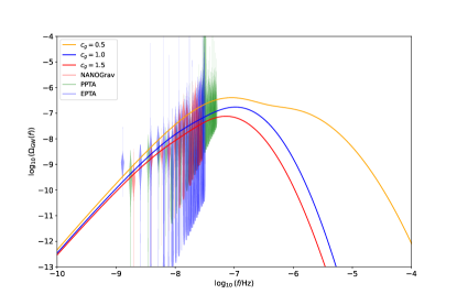
Figure 1: Energy density spectra of SIGW with different speeds $c_{g}$ as a function of GW frequency. As an illustration, we have fixed other parameters as $f_{*}=10^{-7}\,\mathrm{Hz}$, $A=0.2$, and $\Delta=1$.

In Fourier space, the Bardeen potential $\Phi_{\mathbf{k}}$ is related to the primordial curvature perturbations $\zeta_{\mathbf{k}}$ as $\Phi_{\mathbf{k}}=2\zeta_{\mathbf{k}}/3$. This relationship connects the scalar perturbations to the gravitational potential. The solution for tensor perturbations can be expressed as

$$h_{\mathbf{k}}(\eta)=\frac{4}{a(\eta)}\int^{\eta}{\mathrm{d}}\bar{\eta}G_{\mathbf{k}}(\eta,\bar{\eta})a(\bar{\eta})S_{\mathbf{k}}(\bar{\eta}),$$ (7)

where the Green function $G_{\mathbf{k}}(\eta,\bar{\eta})$ is given by Li and Guo (2023)

$$G_{\mathbf{k}}(\eta,\bar{\eta})=\frac{1}{k}\sin[c_{g}k(\eta-\bar{\eta})].$$ (8)

The power spectrum of tensor perturbations is described by the following expression

$$\langle h_{\mathbf{k}}(\eta)h_{\mathbf{k}^{\prime}}(\eta)\rangle=\frac{2\pi^{2}}{k^{3}}\delta^{(3)}(\mathbf{k}+\mathbf{k}^{\prime})\mathcal{P}_{h}(\eta,k),$$ (9)

where the delta function $\delta^{(3)}(\mathbf{k}+\mathbf{k}^{\prime})$ enforces momentum conservation, ensuring that the total momentum of the perturbations is conserved and the factor of $2\pi^{2}/k^{3}$ accounts for the normalization of the power spectrum. Therefore, the power spectrum of tensor perturbations takes the form Ananda et al. (2007); Baumann et al. (2007); Kohri and Terada (2018); Espinosa et al. (2018)

$$\mathcal{P}_{h}(k,\eta) =4\int_{0}^{\infty}\mathrm{d}v\int_{|1-v|}^{1+v}\mathrm{d}u\bigg{[}\left(\frac{4v^{2}-(1+v^{2}-u^{2})^{2}}{4vu}\right)^{2}$$ (10)

$$\times I_{\rm RD}^{2}(u,v,c_{g})\mathcal{P}_{\zeta}(kv)\mathcal{P}_{\zeta}(ku)\bigg{]},$$

where $u=|\mathbf{k}-\tilde{\mathbf{k}}|/k$, $v=\tilde{k}/k$ and $I_{\rm RD}$ is the integral kernel which can be found in Ref. Li and Guo (2023). The characterization of SGWBs often involves quantifying the energy density per logarithmic frequency interval relative to the critical density $\rho_{c}(\eta)$. This quantity, denoted as $\Omega_{\mathrm{GW}}(k,\eta)$, can be expressed as Thrane and Romano (2013)

$$\Omega_{\mathrm{GW}}(k,\eta)=\frac{1}{\rho_{c}(\eta)}\frac{\mathrm{d}\rho_{\mathrm{GW}}(k,\eta)}{\mathrm{d}\ln k}=\frac{k^{3}}{48\pi^{2}}\left(\frac{k}{\mathcal{H}}\right)^{2}\overline{\left\langle\left|h_{\mathbf{k}}(\eta)\right|^{2}\right\rangle}.$$ (11)

Notice that the term $\overline{\left\langle\left|h_{\mathbf{k}}(\eta)\right|^{2}\right\rangle}$ corresponds to an average taken over a few wavelengths. In the radiation-dominated era, GWs are produced by curvature perturbations. At the epoch of matter-radiation equality, the density parameter of GW is denoted as $\Omega_{\mathrm{GW}}(k)=\Omega_{\mathrm{GW}}(k,\eta\rightarrow\infty)$. Therefore, the expression for the energy density of GWs $\Omega_{\mathrm{GW}}(k)$ can be written as Espinosa et al. (2018); Li and Guo (2023)

$$\Omega_{\mathrm{GW}}(k)=\int_{0}^{\infty}\mathrm{d}v\int_{|1-v|}^{1+v}\mathrm{d}u\mathcal{T}(u,v,c_{g}){P}_{\zeta}(vk){P}_{\zeta}(uk),$$ (12)

where the transfer function $\mathcal{T}$ is given by

$$\mathcal{T}(u,v,c_{g}) =\frac{3\left[4v^{2}-\left(v^{2}-u^{2}+1\right)^{2}\right]^{2}\left(v^{2}+u^{2}-3c_{g}^{2}\right)^{2}}{1024v^{8}u^{8}}$$ (13)

$$\times \Bigg{\{}\left[\left(v^{2}+u^{2}-3c_{g}^{2}\right)\ln\left(\left|\frac{3c_{g}^{2}-(v+u)^{2}}{3c_{g}^{2}-(v-u)^{2}}\right|\right)-4vu\right]^{2}$$

$$~{}~{}~{}+\pi^{2}\left(v^{2}+u^{2}-3c_{g}^{2}\right)^{2}\Theta(v+u-\sqrt{3}c_{g})\Bigg{\}}.$$

Here, $\Theta$ denotes the Heaviside theta function. In the case $c_{g}=1$, the SIGWs propagate at the speed of light and the result is reduced to the results in Ref. Kohri and Terada (2018) as predicted by general relativity. Using the relationship between frequency $f$ and the wavenumber $k$, $f=k/2\pi$, one can derive the spectrum of SIGWs at the present time to be

$$\Omega_{\mathrm{GW},0}(f)=\Omega_{\mathrm{r},0}\left[\frac{g_{*,r}(T)}{g_{*,r}\left(T_{\mathrm{eq}}\right)}\right]\left[\frac{g_{*,s}\left(T_{\mathrm{eq}}\right)}{g_{*,s}(T)}\right]^{\frac{4}{3}}\Omega_{\mathrm{GW}}(k),$$ (14)

where $g_{*,s}$ and $g_{*,r}$ correspond to the effective degrees of freedom for entropy density and radiation, respectively. Additionally, $\Omega_{r,0}$ is the present energy density fraction of radiation. To demonstrate the method, we consider a common power spectrum for the curvature perturbation ${P}_{\zeta}$, which is characterized by a lognormal shape

$${P}_{\zeta}(k)=\frac{A}{\sqrt{2\pi}\Delta}\exp\left(-\frac{\ln^{2}(k/k_{*})}{2\Delta^{2}}\right),$$ (15)

where $A$ represents the amplitude of the power spectrum, $k_{*}$ is the characteristic scale that determines the peak location, and $\Delta$ corresponds to the width of the spectrum.

Methodology and result. In this study, we jointly employ PTA data from the EPTA DR2 Antoniadis et al. (2023a), PPTA DR3 Zic et al. (2023), and NANOGrav 15-year data set Agazie et al. (2023a), to rigorously constrain the speed of SIGWs using the Bayesian inference method. In particular, we make use of the amplitude values from the free spectrum obtained by each PTA without considering spatial correlations. It’s worth noting that deviations in the speed of GWs result in variations in the Hellings-Downs Hellings and Downs (1983) correlations. While a comprehensive analysis should consider this effect, the current sensitivity of PTAs poses challenges in distinguishing the deviation from Hellings-Downs correlations due to varying speeds of gravitational waves, as discussed in Bi et al. (2023a). Consequently, we concentrate on dominant information from auto-correlations, neglecting cross-correlations, and emphasize the energy density spectrum’s alteration due to the speed deviation of SIGWs from the speed of light.

The dedicated efforts of PTA collaborations have spanned over a decade. Specifically, the EPTA DR2 includes data from $25$ pulsars over a timespan of $24.7$ years Antoniadis et al. (2023a). The PPTA DR3 comprises observations of $32$ pulsars spanning up to $18$ years Zic et al. (2023), while the NANOGrav 15-year data set encompasses observations from $68$ pulsars over a timespan of $16.03$ years Agazie et al. (2023a). These PTA data sets collectively reveal a stochastic signal consistent with the anticipated Hellings-Downs spatial correlations for an SGWB. Assuming this signal originates from GWs, it is expected to share similar characteristics across these PTAs. Therefore, we merge observations from NANOGrav, PPTA, and EPTA to enhance precision in estimating model parameters, opting for a collaborative approach rather than analyzing each PTA individually. The sensitivity of a PTA initiates at a frequency of $1/T_{\mathrm{obs}}$, where $T_{\mathrm{obs}}$ denotes the observational timespan. The EPTA, PPTA, and NANOGrav collaborations adopt $24$ Antoniadis et al. (2023d), $28$ Reardon et al. (2023), and $14$ Agazie et al. (2023b) frequencies in their search for the SGWB signal, respectively. Through the combination of data from these PTAs, we analyze a total of $66$ frequency components within the free spectrum, covering the range from $1.28$ nHz to $49.1$ nHz. In Fig. 1, we present a visual representation of the data utilized in our analyses, illustrating the energy density of SIGWs for various values of $c_{g}$, while fixing $f_{*}=10^{-7}\,\mathrm{Hz}$, $A=0.2$, and $\Delta=1$.

We initiate our analysis by utilizing the posterior data of time delay $d(f)$, provided by each PTA. The power spectrum $S(f)$ is linked to the time delay through

$$S(f)=d(f)^{2}\,T_{\mathrm{obs}}.$$ (16)

With the provided time delay data, the energy density of the free spectrum can be computed by

$$\hat{\Omega}_{\mathrm{GW}}(f)=\frac{2\pi^{2}}{3H_{0}^{2}}f^{2}h_{c}^{2}(f)=\frac{8\pi^{4}}{H_{0}^{2}}T_{\mathrm{obs}}f^{5}d^{2}(f),$$ (17)

where $H_{0}$ represents the Hubble constant with value taken from Planck Aghanim et al. (2020). The characteristic strain, $h_{c}(f)$, is given by

$$h_{c}^{2}(f)=12\pi^{2}f^{3}S(f).$$ (18)

For every observed frequency $f_{i}$, we utilize the obtained posteriors of $\hat{\Omega}_{\mathrm{GW}}(f_{i})$ as described above, to estimate the corresponding kernel density, $\mathcal{L}_{i}$. Hence, the overall log-likelihood is the sum of the individual log-likelihoods, and it is expressed as Moore and Vecchio (2021); Lamb et al. (2023); Liu et al. (2023c); Wu et al. (2023d); Jin et al. (2023); Liu et al. (2023b)

$$\ln\mathcal{L}(\Lambda)=\sum_{i=1}^{66}\ln\mathcal{L}_{i}(\Omega_{\mathrm{GW}}(f_{i},\Lambda)).$$ (19)

Here, the set of four model parameters is denoted as $\Lambda\equiv\{f_{*},A,\Delta,c_{g}\}$. To explore the parameter space, we utilize the dynesty Speagle (2020) sampler, which is accessible in the Bilby Ashton et al. (2019); Romero-Shaw et al. (2020) package.

Parameter	$\log_{10}(f_{*}/\mathrm{Hz})$	$\log_{10}A$	$\Delta$	$c_{g}$
Prior	${\mathcal{U}}(-8,-2)$	${\mathcal{U}}(-2,2)$	${\mathcal{U}}(0.05,5)$	${\mathcal{U}}(0.1,2)$
Result	$\gtrsim-6.4$	$0.61^{+0.74}_{-1.09}$	$3.57^{+0.84}_{-1.58}$	$\gtrsim 0.61$

Table 1: Priors and results for the model parameters $\Lambda\equiv\{f_{*},A,\Delta,c_{g}\}$. We use ${\mathcal{U}}$ to denote the uniform distribution and quote the result of each parameter with the median and a $90\%$ equal-tail credible interval.

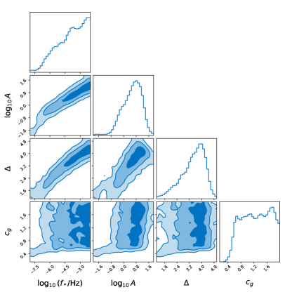
Figure 2: Posterior distributions for the model parameters $\Lambda\equiv\{f_{*},A,\Delta,c_{g}\}$ obtained from the combined PTA data of EPTA DR2, PPTA DR3, and NANOGrav 15-yr data set. We show the $1\sigma$, $2\sigma$, and $3\sigma$ credible regions as contours in the two-dimensional plot.

In our analysis, we employ uniform priors for each parameter: $\log_{10}(f_{*}/\mathrm{Hz})$ in the range $[-8,-2]$, $\log_{10}A$ in the range $[-2,2]$, $\Delta$ in the range $[0.05,5]$, and $c_{g}$ in the range $[0.1,2]$. The posterior distributions for these model parameters are illustrated in Fig. 2. Specifically, we find $\log_{10}A=0.61^{+0.74}_{-1.09}$ and $\Delta=3.57^{+0.84}_{-1.58}$. Unless specified, we quote results using the median value and $90\%$ equal-tail credible interval. Additionally, we find $\log_{10}(f_{*}/\mathrm{Hz})\gtrsim-6.4$ and $c_{g}\gtrsim 0.61$ at a $95\%$ credible interval. A concise summary of priors and results for the model parameters is provided in Table 1. It is important to note that the obtained constraint is consistent with the prediction of general relativity ($c_{g}=1$) at a $90\%$ credible interval.

Conclusion and discussion. The speed of GWs has been a topic of great interest in the field of astrophysics and cosmology due to its profound implications for our understanding of the fundamental laws of the Universe. It represents a key parameter that directly influences the behavior and propagation of GW. In the theory of general relativity, GWs are predicted to propagate at the speed of light. Notably, the binary merger event GW170817 observed by LIGO and Virgo has constrained the propagation speed of GWs as $|1-v|\lesssim 10^{-15}$ at the high frequency of $f\sim 100\mathrm{~{}Hz}$. However, the velocity constraint observed at high frequencies may not necessarily apply to the lower frequency range. Thus, an independent examination of velocity constraints within the lower frequency band, accessible through PTAs, becomes crucial.

In this letter, we conduct a comprehensive analysis by jointly utilizing PTA data from the EPTA DR2 Antoniadis et al. (2023a), PPTA DR3 Zic et al. (2023), and NANOGrav 15-year data set Agazie et al. (2023a) to investigate the speed of the SIGWs, assuming that the stochastic signal observed by recent PTA collaborations originates from the SIGWs. The analysis suggests that, to be consistent with PTA observations, the speed of SIGWs should be $c_{g}\gtrsim 0.61$ at a $95\%$ credible interval. Moreover, the obtained constraint is consistent with the prediction of general relativity ($c_{g}=1$) at a $90\%$ credible interval.

The results derived from the current PTA data exhibit large uncertainties, underscoring the necessity for further investigation to refine our understanding of the fundamental nature of gravity. With the continuous advancement of GW detection technology and precision, PTAs will continue to play a crucial role in unraveling the mysteries of the cosmos and exploring the boundaries of our current theories. The ongoing development of next-generation PTA projects, such as the Square Kilometre Array Lazio (2013), holds immense promise. Our findings have underscored the significant capacity of PTAs in probing the speed of SIGWs.

Acknowledgments. ZCC is supported by the National Natural Science Foundation of China (Grant No. 12247176 and No. 12247112) and the China Postdoctoral Science Foundation Fellowship No. 2022M710429. JL is supported by the Natural Science Foundation of Shandong Province (grant No. ZR2021QA073) and Research Start-up Fund of QUST (grant No. 1203043003587). LL is supported by the National Natural Science Foundation of China (Grant No. 12247112 and No. 12247176) and the China Postdoctoral Science Foundation Fellowship No. 2023M730300. ZY is supported by the National Natural Science Foundation of China under Grant No. 12205015.

References

- Abbott et al. (2019a) B. P. Abbott et al. (LIGO Scientific, Virgo), Phys. Rev. X 9, 031040 (2019a), arXiv:1811.12907 [astro-ph.HE] .
- Abbott et al. (2021a) R. Abbott et al. (LIGO Scientific, Virgo), Phys. Rev. X 11, 021053 (2021a), arXiv:2010.14527 [gr-qc] .
- Abbott et al. (2023a) R. Abbott et al. (KAGRA, VIRGO, LIGO Scientific), Phys. Rev. X 13, 041039 (2023a), arXiv:2111.03606 [gr-qc] .
- Abbott et al. (2019b) B. P. Abbott et al. (LIGO Scientific, Virgo), Phys. Rev. D 100, 104036 (2019b), arXiv:1903.04467 [gr-qc] .
- Abbott et al. (2021b) R. Abbott et al. (LIGO Scientific, Virgo), Phys. Rev. D 103, 122002 (2021b), arXiv:2010.14529 [gr-qc] .
- Abbott et al. (2021c) R. Abbott et al. (LIGO Scientific, VIRGO, KAGRA), (2021c), arXiv:2112.06861 [gr-qc] .
- Abbott et al. (2019c) B. P. Abbott et al. (LIGO Scientific, Virgo), Astrophys. J. Lett. 882, L24 (2019c), arXiv:1811.12940 [astro-ph.HE] .
- Chen et al. (2019) Z.-C. Chen, F. Huang, and Q.-G. Huang, Astrophys. J. 871, 97 (2019), arXiv:1809.10360 [gr-qc] .
- Chen and Huang (2020) Z.-C. Chen and Q.-G. Huang, JCAP 08, 039 (2020), arXiv:1904.02396 [astro-ph.CO] .
- Abbott et al. (2021d) R. Abbott et al. (LIGO Scientific, Virgo), Astrophys. J. Lett. 913, L7 (2021d), arXiv:2010.14533 [astro-ph.HE] .
- Chen et al. (2022a) Z.-C. Chen, C. Yuan, and Q.-G. Huang, Phys. Lett. B 829, 137040 (2022a), arXiv:2108.11740 [astro-ph.CO] .
- Abbott et al. (2023b) R. Abbott et al. (KAGRA, VIRGO, LIGO Scientific), Phys. Rev. X 13, 011048 (2023b), arXiv:2111.03634 [astro-ph.HE] .
- Chen et al. (2023a) Z.-C. Chen, S.-S. Du, Q.-G. Huang, and Z.-Q. You, JCAP 03, 024 (2023a), arXiv:2205.11278 [astro-ph.CO] .
- Liu et al. (2023a) L. Liu, Z.-Q. You, Y. Wu, and Z.-C. Chen, Phys. Rev. D 107, 063035 (2023a), arXiv:2210.16094 [astro-ph.CO] .
- Zheng et al. (2023) L.-M. Zheng, Z. Li, Z.-C. Chen, H. Zhou, and Z.-H. Zhu, Phys. Lett. B 838, 137720 (2023), arXiv:2212.05516 [astro-ph.CO] .
- You et al. (2023a) Z.-Q. You, Z.-C. Chen, L. Liu, Z. Yi, X.-J. Liu, Y. Wu, and Y. Gong, (2023a), arXiv:2306.12950 [astro-ph.CO] .
- Sazhin (1978) M. V. Sazhin, Soviet Astronomy 22, 36 (1978).
- Detweiler (1979) S. L. Detweiler, Astrophys. J. 234, 1100 (1979).
- Foster and Backer (1990) R. S. Foster and D. C. Backer, Astrophys. J. 361, 300 (1990).
- Li et al. (2019) J. Li, Z.-C. Chen, and Q.-G. Huang, Sci. China Phys. Mech. Astron. 62, 110421 (2019), [Erratum: Sci.China Phys.Mech.Astron. 64, 250451 (2021)], arXiv:1907.09794 [astro-ph.CO] .
- Vagnozzi (2021) S. Vagnozzi, Mon. Not. Roy. Astron. Soc. 502, L11 (2021), arXiv:2009.13432 [astro-ph.CO] .
- Chen et al. (2021) Z.-C. Chen, C. Yuan, and Q.-G. Huang, Sci. China Phys. Mech. Astron. 64, 120412 (2021), arXiv:2101.06869 [astro-ph.CO] .
- Wu et al. (2022a) Y.-M. Wu, Z.-C. Chen, and Q.-G. Huang, Astrophys. J. 925, 37 (2022a), arXiv:2108.10518 [astro-ph.CO] .
- Chen et al. (2022b) Z.-C. Chen, Y.-M. Wu, and Q.-G. Huang, Commun. Theor. Phys. 74, 105402 (2022b), arXiv:2109.00296 [astro-ph.CO] .
- Sakharov et al. (2021) A. S. Sakharov, Y. N. Eroshenko, and S. G. Rubin, Phys. Rev. D 104, 043005 (2021), arXiv:2104.08750 [hep-ph] .
- Benetti et al. (2022) M. Benetti, L. L. Graef, and S. Vagnozzi, Phys. Rev. D 105, 043520 (2022), arXiv:2111.04758 [astro-ph.CO] .
- Chen et al. (2022c) Z.-C. Chen, Y.-M. Wu, and Q.-G. Huang, Astrophys. J. 936, 20 (2022c), arXiv:2205.07194 [astro-ph.CO] .
- Ashoorioon et al. (2022) A. Ashoorioon, K. Rezazadeh, and A. Rostami, Phys. Lett. B 835, 137542 (2022), arXiv:2202.01131 [astro-ph.CO] .
- Wu et al. (2022b) Y.-M. Wu, Z.-C. Chen, Q.-G. Huang, X. Zhu, N. D. R. Bhat, Y. Feng, G. Hobbs, R. N. Manchester, C. J. Russell, and R. M. Shannon (PPTA), Phys. Rev. D 106, L081101 (2022b), arXiv:2210.03880 [astro-ph.CO] .
- Wu et al. (2023a) Y.-M. Wu, Z.-C. Chen, and Q.-G. Huang, Phys. Rev. D 107, 042003 (2023a), arXiv:2302.00229 [gr-qc] .
- Falxa et al. (2023) M. Falxa et al. (IPTA), Mon. Not. Roy. Astron. Soc. 521, 5077 (2023), arXiv:2303.10767 [gr-qc] .
- Wu et al. (2023b) Y.-M. Wu, Z.-C. Chen, and Q.-G. Huang, JCAP 09, 021 (2023b), arXiv:2305.08091 [hep-ph] .
- Dandoy et al. (2023) V. Dandoy, V. Domcke, and F. Rompineve, SciPost Phys. Core 6, 060 (2023), arXiv:2302.07901 [astro-ph.CO] .
- Madge et al. (2023) E. Madge, E. Morgante, C. Puchades-Ibáñez, N. Ramberg, W. Ratzinger, S. Schenk, and P. Schwaller, JHEP 10, 171 (2023), arXiv:2306.14856 [hep-ph] .
- Yi et al. (2023a) Z. Yi, Z.-Q. You, Y. Wu, Z.-C. Chen, and L. Liu, (2023a), arXiv:2308.14688 [astro-ph.CO] .
- Wu et al. (2023c) Y.-M. Wu, Z.-C. Chen, Y.-C. Bi, and Q.-G. Huang, (2023c), arXiv:2310.07469 [astro-ph.CO] .
- Bi et al. (2023a) Y.-C. Bi, Y.-M. Wu, Z.-C. Chen, and Q.-G. Huang, (2023a), arXiv:2310.08366 [astro-ph.CO] .
- Chen et al. (2023b) Z.-C. Chen, Y.-M. Wu, Y.-C. Bi, and Q.-G. Huang, (2023b), arXiv:2310.11238 [astro-ph.CO] .
- Xu et al. (2023) H. Xu et al., Res. Astron. Astrophys. 23, 075024 (2023), arXiv:2306.16216 [astro-ph.HE] .
- Antoniadis et al. (2023a) J. Antoniadis et al. (EPTA), Astron. Astrophys. 678, A48 (2023a), arXiv:2306.16224 [astro-ph.HE] .
- Antoniadis et al. (2023b) J. Antoniadis et al. (EPTA, InPTA:), Astron. Astrophys. 678, A50 (2023b), arXiv:2306.16214 [astro-ph.HE] .
- Zic et al. (2023) A. Zic et al., (2023), arXiv:2306.16230 [astro-ph.HE] .
- Reardon et al. (2023) D. J. Reardon et al., Astrophys. J. Lett. 951, L6 (2023), arXiv:2306.16215 [astro-ph.HE] .
- Agazie et al. (2023a) G. Agazie et al. (NANOGrav), Astrophys. J. Lett. 951, L9 (2023a), arXiv:2306.16217 [astro-ph.HE] .
- Agazie et al. (2023b) G. Agazie et al. (NANOGrav), Astrophys. J. Lett. 951, L8 (2023b), arXiv:2306.16213 [astro-ph.HE] .
- Afzal et al. (2023) A. Afzal et al. (NANOGrav), Astrophys. J. Lett. 951, L11 (2023), arXiv:2306.16219 [astro-ph.HE] .
- Antoniadis et al. (2023c) J. Antoniadis et al. (EPTA), (2023c), arXiv:2306.16227 [astro-ph.CO] .
- Bi et al. (2023b) Y.-C. Bi, Y.-M. Wu, Z.-C. Chen, and Q.-G. Huang, Sci. China Phys. Mech. Astron. 66, 120402 (2023b), arXiv:2307.00722 [astro-ph.CO] .
- Zhao et al. (2023) Z.-C. Zhao, Q.-H. Zhu, S. Wang, and X. Zhang, (2023), arXiv:2307.13574 [astro-ph.CO] .
- Wang et al. (2023) S. Wang, Z.-C. Zhao, J.-P. Li, and Q.-H. Zhu, (2023), arXiv:2307.00572 [astro-ph.CO] .
- Liu et al. (2023b) L. Liu, Z.-C. Chen, and Q.-G. Huang, JCAP 11, 071 (2023b), arXiv:2307.14911 [astro-ph.CO] .
- Vagnozzi (2023) S. Vagnozzi, JHEAp 39, 81 (2023), arXiv:2306.16912 [astro-ph.CO] .
- Fu et al. (2023) C. Fu, J. Liu, X.-Y. Yang, W.-W. Yu, and Y. Zhang, (2023), arXiv:2308.15329 [astro-ph.CO] .
- Han et al. (2023) C. Han, K.-P. Xie, J. M. Yang, and M. Zhang, (2023), arXiv:2306.16966 [hep-ph] .
- Kitajima et al. (2023) N. Kitajima, J. Lee, K. Murai, F. Takahashi, and W. Yin, (2023), arXiv:2306.17146 [hep-ph] .
- Franciolini et al. (2023) G. Franciolini, A. Iovino, Junior., V. Vaskonen, and H. Veermae, Phys. Rev. Lett. 131, 201401 (2023), arXiv:2306.17149 [astro-ph.CO] .
- Cai et al. (2023a) Y.-F. Cai, X.-C. He, X.-H. Ma, S.-F. Yan, and G.-W. Yuan, Sci. Bull. 68, 2929 (2023a), arXiv:2306.17822 [gr-qc] .
- Inomata et al. (2023a) K. Inomata, K. Kohri, and T. Terada, (2023a), arXiv:2306.17834 [astro-ph.CO] .
- Li and Xie (2023) S.-P. Li and K.-P. Xie, Phys. Rev. D 108, 055018 (2023), arXiv:2307.01086 [hep-ph] .
- Liu et al. (2023c) L. Liu, Z.-C. Chen, and Q.-G. Huang, (2023c), arXiv:2307.01102 [astro-ph.CO] .
- Abe and Tada (2023) K. T. Abe and Y. Tada, Phys. Rev. D 108, L101304 (2023), arXiv:2307.01653 [astro-ph.CO] .
- Ghosh et al. (2023) T. Ghosh, A. Ghoshal, H.-K. Guo, F. Hajkarim, S. F. King, K. Sinha, X. Wang, and G. White, (2023), arXiv:2307.02259 [astro-ph.HE] .
- Figueroa et al. (2023) D. G. Figueroa, M. Pieroni, A. Ricciardone, and P. Simakachorn, (2023), arXiv:2307.02399 [astro-ph.CO] .
- Yi et al. (2023b) Z. Yi, Q. Gao, Y. Gong, Y. Wang, and F. Zhang, Sci. China Phys. Mech. Astron. 66, 120404 (2023b), arXiv:2307.02467 [gr-qc] .
- Wu et al. (2023d) Y.-M. Wu, Z.-C. Chen, and Q.-G. Huang, (2023d), arXiv:2307.03141 [astro-ph.CO] .
- You et al. (2023b) Z.-Q. You, Z. Yi, and Y. Wu, JCAP 11, 065 (2023b), arXiv:2307.04419 [gr-qc] .
- Antusch et al. (2023) S. Antusch, K. Hinze, S. Saad, and J. Steiner, Phys. Rev. D 108, 095053 (2023), arXiv:2307.04595 [hep-ph] .
- Hosseini Mansoori et al. (2023) S. A. Hosseini Mansoori, F. Felegray, A. Talebian, and M. Sami, JCAP 08, 067 (2023), arXiv:2307.06757 [astro-ph.CO] .
- Jin et al. (2023) J.-H. Jin, Z.-C. Chen, Z. Yi, Z.-Q. You, L. Liu, and Y. Wu, JCAP 09, 016 (2023), arXiv:2307.08687 [astro-ph.CO] .
- Zhang et al. (2023) Z. Zhang, C. Cai, Y.-H. Su, S. Wang, Z.-H. Yu, and H.-H. Zhang, Phys. Rev. D 108, 095037 (2023), arXiv:2307.11495 [hep-ph] .
- Choudhury (2023) S. Choudhury, (2023), arXiv:2307.03249 [astro-ph.CO] .
- Gorji et al. (2023) M. A. Gorji, M. Sasaki, and T. Suyama, Phys. Lett. B 846, 138214 (2023), arXiv:2307.13109 [astro-ph.CO] .
- Das et al. (2023) B. Das, N. Jaman, and M. Sami, Phys. Rev. D 108, 103510 (2023), arXiv:2307.12913 [gr-qc] .
- Yi et al. (2023c) Z. Yi, Z.-Q. You, and Y. Wu, (2023c), arXiv:2308.05632 [astro-ph.CO] .
- Ellis et al. (2023) J. Ellis, M. Fairbairn, G. Franciolini, G. Hütsi, A. Iovino, M. Lewicki, M. Raidal, J. Urrutia, V. Vaskonen, and H. Veermäe, (2023), arXiv:2308.08546 [astro-ph.CO] .
- He et al. (2023) S. He, L. Li, S. Wang, and S.-J. Wang, (2023), arXiv:2308.07257 [hep-ph] .
- Balaji et al. (2023) S. Balaji, G. Domènech, and G. Franciolini, JCAP 10, 041 (2023), arXiv:2307.08552 [gr-qc] .
- Cannizzaro et al. (2023) E. Cannizzaro, G. Franciolini, and P. Pani, (2023), arXiv:2307.11665 [gr-qc] .
- Maji and Park (2024) R. Maji and W.-I. Park, JCAP 01, 015 (2024), arXiv:2308.11439 [hep-ph] .
- Bhaumik et al. (2023) N. Bhaumik, R. K. Jain, and M. Lewicki, Phys. Rev. D 108, 123532 (2023), arXiv:2308.07912 [astro-ph.CO] .
- Zhu et al. (2023) M. Zhu, G. Ye, and Y. Cai, Eur. Phys. J. C 83, 816 (2023), arXiv:2307.16211 [astro-ph.CO] .
- Basilakos et al. (2023) S. Basilakos, D. V. Nanopoulos, T. Papanikolaou, E. N. Saridakis, and C. Tzerefos, (2023), arXiv:2307.08601 [hep-th] .
- Huang et al. (2023) H.-L. Huang, Y. Cai, J.-Q. Jiang, J. Zhang, and Y.-S. Piao, (2023), arXiv:2306.17577 [gr-qc] .
- Jiang et al. (2023) J.-Q. Jiang, Y. Cai, G. Ye, and Y.-S. Piao, (2023), arXiv:2307.15547 [astro-ph.CO] .
- Agazie et al. (2023c) G. Agazie et al. (International Pulsar Timing Array), (2023c), arXiv:2309.00693 [astro-ph.HE] .
- Harigaya et al. (2023) K. Harigaya, K. Inomata, and T. Terada, Phys. Rev. D 108, 123538 (2023), arXiv:2309.00228 [astro-ph.CO] .
- Lozanov et al. (2023) K. D. Lozanov, S. Pi, M. Sasaki, V. Takhistov, and A. Wang, (2023), arXiv:2310.03594 [astro-ph.CO] .
- Choudhury et al. (2023) S. Choudhury, K. Dey, A. Karde, S. Panda, and M. Sami, (2023), arXiv:2310.11034 [astro-ph.CO] .
- Cang et al. (2023) J. Cang, Y. Gao, Y. Liu, and S. Sun, (2023), arXiv:2309.15069 [astro-ph.CO] .
- Mu et al. (2023) B. Mu, J. Liu, G. Cheng, and Z.-K. Guo, (2023), arXiv:2310.20564 [astro-ph.CO] .
- Chen et al. (2023c) Z.-C. Chen, S.-L. Li, P. Wu, and H. Yu, (2023c), arXiv:2312.01824 [astro-ph.CO] .
- Liu et al. (2023d) L. Liu, Y. Wu, and Z.-C. Chen, (2023d), arXiv:2310.16500 [astro-ph.CO] .
- Chao et al. (2023) W. Chao, J.-j. Feng, H.-k. Guo, and T. Li, (2023), arXiv:2312.04017 [hep-ph] .
- Fei (2023) Q. Fei, (2023), arXiv:2310.17199 [gr-qc] .
- Maiti et al. (2024) S. Maiti, D. Maity, and L. Sriramkumar, (2024), arXiv:2401.01864 [gr-qc] .
- Belotsky et al. (2014) K. M. Belotsky, A. D. Dmitriev, E. A. Esipova, V. A. Gani, A. V. Grobov, M. Y. Khlopov, A. A. Kirillov, S. G. Rubin, and I. V. Svadkovsky, Mod. Phys. Lett. A 29, 1440005 (2014), arXiv:1410.0203 [astro-ph.CO] .
- Wang et al. (2018) S. Wang, Y.-F. Wang, Q.-G. Huang, and T. G. F. Li, Phys. Rev. Lett. 120, 191102 (2018), arXiv:1610.08725 [astro-ph.CO] .
- Carr et al. (2016) B. Carr, F. Kuhnel, and M. Sandstad, Phys. Rev. D 94, 083504 (2016), arXiv:1607.06077 [astro-ph.CO] .
- Garcia-Bellido and Ruiz Morales (2017) J. Garcia-Bellido and E. Ruiz Morales, Phys. Dark Univ. 18, 47 (2017), arXiv:1702.03901 [astro-ph.CO] .
- Carr et al. (2017) B. Carr, M. Raidal, T. Tenkanen, V. Vaskonen, and H. Veermäe, Phys. Rev. D 96, 023514 (2017), arXiv:1705.05567 [astro-ph.CO] .
- Germani and Prokopec (2017) C. Germani and T. Prokopec, Phys. Dark Univ. 18, 6 (2017), arXiv:1706.04226 [astro-ph.CO] .
- Liu et al. (2019a) L. Liu, Z.-K. Guo, and R.-G. Cai, Phys. Rev. D 99, 063523 (2019a), arXiv:1812.05376 [astro-ph.CO] .
- Chen and Huang (2018) Z.-C. Chen and Q.-G. Huang, Astrophys. J. 864, 61 (2018), arXiv:1801.10327 [astro-ph.CO] .
- Liu et al. (2019b) L. Liu, Z.-K. Guo, and R.-G. Cai, Eur. Phys. J. C 79, 717 (2019b), arXiv:1901.07672 [astro-ph.CO] .
- Fu et al. (2019) C. Fu, P. Wu, and H. Yu, Phys. Rev. D 100, 063532 (2019), arXiv:1907.05042 [astro-ph.CO] .
- Wang et al. (2019) S. Wang, T. Terada, and K. Kohri, Phys. Rev. D 99, 103531 (2019), [Erratum: Phys.Rev.D 101, 069901 (2020)], arXiv:1903.05924 [astro-ph.CO] .
- Liu et al. (2020a) J. Liu, Z.-K. Guo, and R.-G. Cai, Phys. Rev. D 101, 023513 (2020a), arXiv:1908.02662 [astro-ph.CO] .
- Cai et al. (2020a) R.-G. Cai, Z.-K. Guo, J. Liu, L. Liu, and X.-Y. Yang, JCAP 06, 013 (2020a), arXiv:1912.10437 [astro-ph.CO] .
- Liu et al. (2020b) L. Liu, Z.-K. Guo, R.-G. Cai, and S. P. Kim, Phys. Rev. D 102, 043508 (2020b), arXiv:2001.02984 [astro-ph.CO] .
- Fu et al. (2020) C. Fu, P. Wu, and H. Yu, Phys. Rev. D 102, 043527 (2020), arXiv:2006.03768 [astro-ph.CO] .
- Wu (2020) Y. Wu, Phys. Rev. D 101, 083008 (2020), arXiv:2001.03833 [astro-ph.CO] .
- De Luca et al. (2021a) V. De Luca, V. Desjacques, G. Franciolini, P. Pani, and A. Riotto, Phys. Rev. Lett. 126, 051101 (2021a), arXiv:2009.01728 [astro-ph.CO] .
- Vaskonen and Veermäe (2021) V. Vaskonen and H. Veermäe, Phys. Rev. Lett. 126, 051303 (2021), arXiv:2009.07832 [astro-ph.CO] .
- De Luca et al. (2021b) V. De Luca, G. Franciolini, and A. Riotto, Phys. Rev. Lett. 126, 041303 (2021b), arXiv:2009.08268 [astro-ph.CO] .
- Domènech et al. (2021) G. Domènech, C. Lin, and M. Sasaki, JCAP 04, 062 (2021), [Erratum: JCAP 11, E01 (2021)], arXiv:2012.08151 [gr-qc] .
- Domènech and Pi (2022) G. Domènech and S. Pi, Sci. China Phys. Mech. Astron. 65, 230411 (2022), arXiv:2010.03976 [astro-ph.CO] .
- Hütsi et al. (2021) G. Hütsi, M. Raidal, V. Vaskonen, and H. Veermäe, JCAP 03, 068 (2021), arXiv:2012.02786 [astro-ph.CO] .
- Kawai and Kim (2021) S. Kawai and J. Kim, Phys. Rev. D 104, 083545 (2021), arXiv:2108.01340 [astro-ph.CO] .
- Braglia et al. (2021) M. Braglia, J. Garcia-Bellido, and S. Kuroyanagi, JCAP 12, 012 (2021), arXiv:2110.07488 [astro-ph.CO] .
- Cai et al. (2021) R.-G. Cai, C. Chen, and C. Fu, Phys. Rev. D 104, 083537 (2021), arXiv:2108.03422 [astro-ph.CO] .
- Liu et al. (2023e) L. Liu, X.-Y. Yang, Z.-K. Guo, and R.-G. Cai, JCAP 01, 006 (2023e), arXiv:2112.05473 [astro-ph.CO] .
- Braglia et al. (2023) M. Braglia, J. Garcia-Bellido, and S. Kuroyanagi, Mon. Not. Roy. Astron. Soc. 519, 6008 (2023), arXiv:2201.13414 [astro-ph.CO] .
- Chen et al. (2023d) Z.-C. Chen, S. P. Kim, and L. Liu, Commun. Theor. Phys. 75, 065401 (2023d), arXiv:2210.15564 [gr-qc] .
- Inomata et al. (2023b) K. Inomata, M. Braglia, X. Chen, and S. Renaux-Petel, JCAP 04, 011 (2023b), [Erratum: JCAP 09, E01 (2023)], arXiv:2211.02586 [astro-ph.CO] .
- Guo et al. (2023) S.-Y. Guo, M. Khlopov, X. Liu, L. Wu, Y. Wu, and B. Zhu, (2023), arXiv:2306.17022 [hep-ph] .
- Cai et al. (2023b) Y. Cai, M. Zhu, and Y.-S. Piao, (2023b), arXiv:2305.10933 [gr-qc] .
- Meng et al. (2023) D.-S. Meng, C. Yuan, and Q.-G. Huang, Sci. China Phys. Mech. Astron. 66, 280411 (2023), arXiv:2212.03577 [astro-ph.CO] .
- Gu et al. (2023) B.-M. Gu, F.-W. Shu, and K. Yang, (2023), arXiv:2307.00510 [astro-ph.CO] .
- Sasaki et al. (2018) M. Sasaki, T. Suyama, T. Tanaka, and S. Yokoyama, Class. Quant. Grav. 35, 063001 (2018), arXiv:1801.05235 [astro-ph.CO] .
- Carr et al. (2021) B. Carr, K. Kohri, Y. Sendouda, and J. Yokoyama, Rept. Prog. Phys. 84, 116902 (2021), arXiv:2002.12778 [astro-ph.CO] .
- Carr and Kuhnel (2020) B. Carr and F. Kuhnel, Ann. Rev. Nucl. Part. Sci. 70, 355 (2020), arXiv:2006.02838 [astro-ph.CO] .
- Ananda et al. (2007) K. N. Ananda, C. Clarkson, and D. Wands, Phys. Rev. D 75, 123518 (2007), arXiv:gr-qc/0612013 .
- Baumann et al. (2007) D. Baumann, P. J. Steinhardt, K. Takahashi, and K. Ichiki, Phys. Rev. D 76, 084019 (2007), arXiv:hep-th/0703290 .
- Garcia-Bellido et al. (2016) J. Garcia-Bellido, M. Peloso, and C. Unal, JCAP 12, 031 (2016), arXiv:1610.03763 [astro-ph.CO] .
- Inomata et al. (2017) K. Inomata, M. Kawasaki, K. Mukaida, Y. Tada, and T. T. Yanagida, Phys. Rev. D 95, 123510 (2017), arXiv:1611.06130 [astro-ph.CO] .
- Garcia-Bellido et al. (2017) J. Garcia-Bellido, M. Peloso, and C. Unal, JCAP 09, 013 (2017), arXiv:1707.02441 [astro-ph.CO] .
- Kohri and Terada (2018) K. Kohri and T. Terada, Phys. Rev. D 97, 123532 (2018), arXiv:1804.08577 [gr-qc] .
- Cai et al. (2019) R.-g. Cai, S. Pi, and M. Sasaki, Phys. Rev. Lett. 122, 201101 (2019), arXiv:1810.11000 [astro-ph.CO] .
- Lu et al. (2019) Y. Lu, Y. Gong, Z. Yi, and F. Zhang, JCAP 12, 031 (2019), arXiv:1907.11896 [gr-qc] .
- Yuan et al. (2020a) C. Yuan, Z.-C. Chen, and Q.-G. Huang, Phys. Rev. D 101, 043019 (2020a), arXiv:1910.09099 [astro-ph.CO] .
- Chen et al. (2020) Z.-C. Chen, C. Yuan, and Q.-G. Huang, Phys. Rev. Lett. 124, 251101 (2020), arXiv:1910.12239 [astro-ph.CO] .
- Xu et al. (2020) W.-T. Xu, J. Liu, T.-J. Gao, and Z.-K. Guo, Phys. Rev. D 101, 023505 (2020), arXiv:1907.05213 [astro-ph.CO] .
- Cai et al. (2020b) R.-G. Cai, S. Pi, and M. Sasaki, Phys. Rev. D 102, 083528 (2020b), arXiv:1909.13728 [astro-ph.CO] .
- Yuan et al. (2020b) C. Yuan, Z.-C. Chen, and Q.-G. Huang, Phys. Rev. D 101, 063018 (2020b), arXiv:1912.00885 [astro-ph.CO] .
- Yi et al. (2021a) Z. Yi, Y. Gong, B. Wang, and Z.-h. Zhu, Phys. Rev. D 103, 063535 (2021a), arXiv:2007.09957 [gr-qc] .
- Yi et al. (2021b) Z. Yi, Q. Gao, Y. Gong, and Z.-h. Zhu, Phys. Rev. D 103, 063534 (2021b), arXiv:2011.10606 [astro-ph.CO] .
- Liu et al. (2020c) J. Liu, Z.-K. Guo, and R.-G. Cai, Phys. Rev. D 101, 083535 (2020c), arXiv:2003.02075 [astro-ph.CO] .
- Gao et al. (2021) Q. Gao, Y. Gong, and Z. Yi, Nucl. Phys. B 969, 115480 (2021), arXiv:2012.03856 [gr-qc] .
- Yi and Zhu (2022) Z. Yi and Z.-H. Zhu, JCAP 05, 046 (2022), arXiv:2105.01943 [gr-qc] .
- Yi (2023) Z. Yi, JCAP 03, 048 (2023), arXiv:2206.01039 [gr-qc] .
- Yi and Fei (2023) Z. Yi and Q. Fei, Eur. Phys. J. C 83, 82 (2023), arXiv:2210.03641 [astro-ph.CO] .
- Yuan et al. (2019) C. Yuan, Z.-C. Chen, and Q.-G. Huang, Phys. Rev. D 100, 081301 (2019), arXiv:1906.11549 [astro-ph.CO] .
- Inui et al. (2023) R. Inui, S. Jaraba, S. Kuroyanagi, and S. Yokoyama, (2023), arXiv:2311.05423 [astro-ph.CO] .
- Domènech (2021) G. Domènech, Universe 7, 398 (2021), arXiv:2109.01398 [gr-qc] .
- Abbott et al. (2017a) B. P. Abbott et al. (LIGO Scientific, Virgo), Phys. Rev. Lett. 119, 161101 (2017a), arXiv:1710.05832 [gr-qc] .
- Abbott et al. (2017b) B. P. Abbott et al. (LIGO Scientific, Virgo, Fermi-GBM, INTEGRAL), Astrophys. J. Lett. 848, L13 (2017b), arXiv:1710.05834 [astro-ph.HE] .
- Weinberg (2004) S. Weinberg, Phys. Rev. D 69, 023503 (2004), arXiv:astro-ph/0306304 .
- Watanabe and Komatsu (2006) Y. Watanabe and E. Komatsu, Phys. Rev. D 73, 123515 (2006), arXiv:astro-ph/0604176 .
- Li and Guo (2023) J. Li and G.-H. Guo, (2023), arXiv:2312.04589 [gr-qc] .
- Espinosa et al. (2018) J. R. Espinosa, D. Racco, and A. Riotto, JCAP 09, 012 (2018), arXiv:1804.07732 [hep-ph] .
- Thrane and Romano (2013) E. Thrane and J. D. Romano, Phys. Rev. D 88, 124032 (2013), arXiv:1310.5300 [astro-ph.IM] .
- Hellings and Downs (1983) R. w. Hellings and G. s. Downs, Astrophys. J. Lett. 265, L39 (1983).
- Antoniadis et al. (2023d) J. Antoniadis et al. (EPTA, InPTA:), Astron. Astrophys. 678, A50 (2023d), arXiv:2306.16214 [astro-ph.HE] .
- Aghanim et al. (2020) N. Aghanim et al. (Planck), Astron. Astrophys. 641, A6 (2020), [Erratum: Astron.Astrophys. 652, C4 (2021)], arXiv:1807.06209 [astro-ph.CO] .
- Moore and Vecchio (2021) C. J. Moore and A. Vecchio, Nature Astron. 5, 1268 (2021), arXiv:2104.15130 [astro-ph.CO] .
- Lamb et al. (2023) W. G. Lamb, S. R. Taylor, and R. van Haasteren, Phys. Rev. D 108, 103019 (2023), arXiv:2303.15442 [astro-ph.HE] .
- Speagle (2020) J. S. Speagle, Mon. Not. Roy. Astron. Soc. 493, 3132 (2020), arXiv:1904.02180 [astro-ph.IM] .
- Ashton et al. (2019) G. Ashton et al., Astrophys. J. Suppl. 241, 27 (2019), arXiv:1811.02042 [astro-ph.IM] .
- Romero-Shaw et al. (2020) I. M. Romero-Shaw et al., Mon. Not. Roy. Astron. Soc. 499, 3295 (2020), arXiv:2006.00714 [astro-ph.IM] .
- Lazio (2013) T. J. W. Lazio, Class. Quant. Grav. 30, 224011 (2013).