Automatic Tuning of Denoising Algorithms Parameters without Ground Truth

Abstract

Denoising is omnipresent in image processing. It is usually addressed with algorithms relying on a set of hyperparameters that control the quality of the recovered image. Manual tuning of those parameters can be a daunting task, which calls for the development of automatic tuning methods. Given a denoising algorithm, the best set of parameters is the one that minimizes the error between denoised and ground-truth images. Clearly, this ideal approach is unrealistic, as the ground-truth images are unknown in practice. In this work, we propose unsupervised cost functions — i.e., that only require the noisy image — that allow us to reach this ideal gold standard performance. Specifically, the proposed approach makes it possible to obtain an average PSNR output within less than 1% of the best achievable PSNR.

I Introduction

Noise is inherent to any imaging device. It comes from a variety of sources and is modeled in a variety of ways. When considering additive noise, the corrupted measurements $\mathbf{y}\in\mathbb{R}^{N}$ follow the model :

$$\mathbf{y}=\mathbf{x}+\mathbf{n},$$ (1)

with $\mathbf{x}\in\mathbb{R}^{N}$ the clean image we wish to recover, and $\mathbf{n}\in\mathbb{R}^{N}$ the noise. Many denoising algorithms, denoted $A_{\bm{\uptheta}}$, have been proposed to address this task and provide estimates given by $A_{\bm{\uptheta}}(\mathbf{y})$, e.g, [1, 2, 3], to cite few. The quality of these estimates depends on the chosen parameters $\bm{\uptheta}\in\mathbb{R}^{d}$. In practice, however, manual tuning of these parameters is far from being trivial, even for low numbers of parameters such as two or three. As such, finding ways to automatically tune these parameters is of major importance and constitutes an active area of research. Most existing approaches use a mapping $\bm{\Theta}_{\bm{\uplambda}}:\mathbf{y}\mapsto\bm{\uptheta}$, itself parameterized by $\bm{\uplambda}\in\mathbb{R}^{d^{\prime}}$, that maps an image and/or its features (e.g., noise level, noise type, image dynamic, image content) to a set of parameters $\bm{\uptheta}$. The best $\bm{\uplambda}$, i.e. $\bm{\uplambda}^{*}$, is found by minimizing the expectancy $\underset{}{\mathbb{E}}$ of a discrepancy measure $\mathcal{L}(\cdot,\cdot)$ between the denoised images and ground truth images:

$${\bm{\uplambda}}^{*}:=\arg\min_{\bm{\uplambda}\in\mathbb{R}^{d^{\prime}}}\underset{(\mathbf{x},\mathbf{y})}{\mathbb{E}}[\mathcal{L}(A_{\bm{\Theta}_{\bm{\uplambda}}(\mathbf{y})}(\mathbf{y}),\mathbf{x})].$$ (2)

There are several possibilities to define $\bm{\Theta}_{\bm{\uplambda}}$ with increasing degree of sophistication:

• $\bm{\Theta}_{\bm{\uplambda}}$ is a constant mapping (i.e., $\bm{\Theta}_{\bm{\uplambda}}(\mathbf{y})=\bm{\uptheta}\in\mathbb{R}^{d}$). Solving (2) then consists in finding a fixed set of parameters $\bm{\uptheta}$ such that, on average, the estimates are good, e.g, [4].

• $\bm{\Theta}_{\bm{\uplambda}}$ is defined using features extracted from $\mathbf{y}$. For instance, $\bm{\Theta}_{\bm{\uplambda}}(\mathbf{y})=\lambda_{1}+\lambda_{2}\hat{\sigma}(\mathbf{y})$ where $\hat{\sigma}(\mathbf{y})$ is an estimator of the noise variance. Here, solving (2) allows us to learn a mapping $\bm{\Theta}_{\bm{\uplambda}}$ that adjusts algorithm parameters according to a known and predefined model, e.g, [5].

• $\bm{\Theta}_{\bm{\uplambda}}$ is a neural network. In this case, solving (2) allows us to learn a mapping $\bm{\Theta}_{\bm{\uplambda}}$ that adjusts algorithm parameters according to an unknown model, e.g, [6, 7]. This greater flexibility comes at the price of a larger number of parameters $\bm{\uplambda}$ to learn.

Typically, all these methods require a dataset and work in a supervised way. Since this is not always feasible, unsupervised alternatives have been developed [8, 9, 10, 11]. The main idea behind these approaches is to define an unsupervised loss (i.e., that does not depend on $\mathbf{x}$) achieving the same minimizers as the supervised counterpart. Nevertheless, constructing $\bm{\Theta}_{\bm{\uplambda}}$ and finding $\bm{\uplambda}$ remains challenging.

To discard the need of defining and training a mapping $\bm{\Theta}_{\bm{\uplambda}}$ on a dataset, one could directly fit ${\bm{\uptheta}}$ on individual images $\mathbf{y}$. The ideal estimate would be:

$$\begin{split}&\mathbf{x}^{*}:=A_{\bm{\uptheta}^{*}}(\mathbf{y})\\ \text{with }&{\bm{\uptheta}}^{*}:=\arg\min_{\bm{\uptheta}\in\mathbb{R}^{d}}\mathcal{C}^{*}_{\mathbf{y}}(\bm{\uptheta})~{},~{}\mathcal{C}^{*}_{\mathbf{y}}(\bm{\uptheta}):=\mathcal{L}(A_{\bm{\uptheta}}(\mathbf{y}),\mathbf{x}).\end{split}$$ (3)

Yet, this formulation is impractical as it requires knowing $\mathbf{x}$ to obtain ${\mathbf{x}}^{*}$. In the following, ${\mathbf{x}}^{*}$ will be our gold standard, that is, the best estimate we can expect for a given image $\mathbf{y}$ and algorithm $A_{\bm{\uptheta}}$. For Gaussian noise, methods such as the famous generalized cross-validation (GCV) [12] and its variants or the Stein’s unbiased risk estimate (SURE) [13], which depends only on the noisy data, can be used in place of the true mean-squared error (MSE). The SURE optimization is, however, challenging in the general case and requires the use of approximations [14] or Monte Carlo approaches [15]. It is noteworthy to mention that other metrics that do not require the reference image have also been proposed [16, 17].

Here, inspired by [8, 9, 10, 11], we propose alternative unsupervised cost functions $\widehat{\mathcal{C}}$ and inference schemes $\widehat{\mathcal{I}}$ such that:

$$\begin{split}&\mathbf{x}^{*}\approx\hat{\mathbf{x}}:=\widehat{\mathcal{I}}(\hat{\bm{\uptheta}},\mathbf{y})\\ \text{with }&\hat{\bm{\uptheta}}:=\arg\min_{\bm{\uptheta}\in\mathbb{R}^{d}}\widehat{\mathcal{C}}_{\mathbf{y}}(\bm{\uptheta}).\end{split}$$ (4)

Let us emphasize that the inference scheme in (4) is not directly $A_{\hat{\bm{\uptheta}}}(\mathbf{y})$. Indeed, as detailed in Section II, the proposed unsupervised cost functions may require adapting the inference scheme. As such, we will systematically specify both the cost function and the inference scheme.

Remark 1

The use of the cost function $\mathcal{C}^{*}$ could be avoided in (3) and replaced with $\mathcal{L}$ directly. We write (3) this way to be consistent with the following unsupervised cost functions $\widehat{\mathcal{C}}$, which don’t reduce to simple discrepancy measures between two images. Moreover, we will use $\cdot^{*}$ and $\widehat{\cdot}$ for supervised and unsupervised objects, respectively.

Paper Outline

The paper is structured as follows. The proposed method is detailed in Section II. Then, in Section III, we deploy our approach to tune the parameters of a recently published denoiser [3] that can handle a variety of noise types. Finally, discussions and conclusions are provided in Section IV.

II Method

Let us start this section by restating the key difference between our approach in Eq. (4) and the more standard one in Eq. (2) (with its unsupervised counterparts [8, 9, 10, 11]). Notably, there is no training phase in (4). We don’t need to create and train a mapping $\bm{\Theta}_{\bm{\uplambda}}$ over a dataset that will then be used to infer estimates on new data. Instead, our inference is done by solving (4) directly for individual images $\mathbf{y}$.

We also emphasize that our aim is not to build a new denoiser, but an automatic way to select hyperparameters of a given denoiser, using only the input noisy image. For illustration purposes, we use the DeQuIP algorithm [3] described in Section II-C.

II-A The Cost Functions and Inference Schemes Definition

We drew our inspiration from existing unsupervised learning methods. Instead of training a denoising neural network $f$ of parameters $\upomega$, say $f_{\bm{\upomega}}$, on noisy-clean pairs $(\mathbf{y},\mathbf{x})$, Noise2Noise (N2N) [8] proposes to train it on pairs of noisy images $(\mathbf{y},\mathbf{y^{\prime}})$ with $\mathbf{y}$ and $\mathbf{y^{\prime}}$ two noisy versions of the same clean image $\mathbf{x}$. Lehtinen et al. [8] showed that for several noise types, $\mathcal{L}$ can be chosen accordingly so that:

$$\mkern-8.0mu\arg\min_{\bm{\upomega}}\underset{(\mathbf{y},\mathbf{y^{\prime}})}{\mathbb{E}}\mathcal{L}(f_{\bm{\upomega}}(\mathbf{y}),\mathbf{y^{\prime}})=\arg\min_{\bm{\upomega}}\underset{(\mathbf{x},\mathbf{y})}{\mathbb{E}}\mathcal{L}(f_{\bm{\upomega}}(\mathbf{y}),\mathbf{x}).$$ (5)

For example, if $\mathbf{y},\mathbf{y^{\prime}}$ are two corrupted versions of $\mathbf{x}$ with independent additive zero-mean noise (i.e., $\mathbf{y}=\mathbf{x}+\mathbf{n}$, $\mathbf{y^{\prime}}=\mathbf{x}+\mathbf{n^{\prime}}$ with $\mathbb{E}[\mathbf{n}]=\mathbb{E}[\mathbf{n^{\prime}}]=\mathbf{0}$), letting $\mathcal{L}$ be the quadratic error leads to (5):

$$\hat{{\bm{\upomega}}}:= \arg\min_{\bm{\upomega}}\underset{(\mathbf{y},\mathbf{\mathbf{y^{\prime}}})}{\mathbb{E}}\|f_{\bm{\upomega}}(\mathbf{y})-\mathbf{y^{\prime}}\|^{2}_{2}$$

$$= \arg\min_{\bm{\upomega}}\underset{(\mathbf{y},\mathbf{x},\mathbf{\mathbf{n}^{\prime}})}{\mathbb{E}}\|f_{\bm{\upomega}}(\mathbf{y})-\mathbf{x}-\mathbf{n^{\prime}}\|^{2}_{2}$$

$$= \arg\min_{\bm{\upomega}}\underset{(\mathbf{y},\mathbf{x},\mathbf{\mathbf{n}^{\prime}})}{\mathbb{E}}\left[\|f_{\bm{\upomega}}(\mathbf{y})-\mathbf{x}\|^{2}_{2}-2\left<f_{\bm{\upomega}}(\mathbf{y})-\mathbf{x},\mathbf{n}^{\prime}\right>\right]$$

$$= \arg\min_{\bm{\upomega}}\underset{(\mathbf{y},\mathbf{x})}{\mathbb{E}}\|f_{\bm{\upomega}}(\mathbf{y})-\mathbf{x}\|^{2}_{2}:=\bm{\upomega}^{*},$$ (6)

where the expectation of the dot product cancels as $\mathbb{E}[\mathbf{n^{\prime}}]=\mathbf{0},$ and $\mathbf{n}$ and $\mathbf{n^{\prime}}$ (i.e., $\mathbf{y}$ and $\mathbf{n^{\prime}}$) are independent.

In practice, training is performed using a finite dataset $\Omega_{I,J}:=\{\mathbf{y}_{i}^{j}=\mathbf{x}_{i}+\mathbf{n}_{i}^{j}\}_{i,j=(1,1)}^{I,J}$. This means that for a noiseless image $\mathbf{x}_{i}$, $J$ noisy versions are available, with additive noises $\mathbf{n}_{i}^{j}$ . As such, the true loss in (5) is replaced by an empirical one. This results in a solution $\hat{\bm{\upomega}}\approx\bm{\upomega}^{*}$ whose quality depends on $I,J$:

• When both $I$ and $J$ are large, the empirical loss yields a good approximation of the true one.

• When $I$ is small (e.g., $I=1$), but $J$ is large, we can expect $f_{\widehat{\bm{\upomega}}}$ to perform well on the training set, but not to generalize well. It will effectively learn to output the mean of the $\mathbf{y}^{j}_{1}$, which is $\mathbf{x}_{1}$.

• When $J$ is small (e.g., $J=2$, with different $\mathbf{n}_{i}^{1}$, $\mathbf{n}_{i}^{2}$ for each $i$), $f_{\widehat{\bm{\upomega}}}$ could overfit the dataset $\Omega_{I,J}$ to the point that we systematically obtain $f_{\widehat{\bm{\upomega}}}(\mathbf{y}^{1}_{i})=\mathbf{y}^{2}_{i},\ f_{\widehat{\bm{\upomega}}}(\mathbf{y}^{2}_{i})=\mathbf{y}^{1}_{i},\ \forall i$. Yet, a large $I$ (e.g., $I=1000$) seems to be sufficient in preventing overfitting as demonstrated by Lehtinen et al, [8]. Other factors can be exploited to avoid overfitting when limited data are available. These include network architecture, image type, noise type, or a low number of parameters relative to image size, $\mathrm{card}({\bm{\upomega}})/P$, with $P$ the number of image pixels [18]. For instance, it has been shown that U-Net-like networks have a hard time recreating noise [19].

• When both $I$ and $J$ are small (e.g., $I=1$, $J=2$), if not carefully designed, $f_{\bm{\upomega}}$ would simply learn to map $\mathbf{y}^{1}_{1}$ to $\mathbf{y}^{2}_{1}$, and vice-versa.

The proposed method, i.e., fitting algorithm parameters to a single image, corresponds to the last extreme case. We argue that if, instead of a neural network (which can recreate noise), we use a denoising algorithm $A_{\bm{\uptheta}}$ with low $\mathrm{card}({\bm{\uptheta}})/P$, we can define:

$$\widehat{\mathcal{C}}^{\mathrm{N2N}}_{\mathbf{y},\mathbf{y^{\prime}}}(\bm{\uptheta}):=\|A_{\bm{\uptheta}}(\mathbf{y})-\mathbf{y^{\prime}}\|^{2}_{2},\,\hat{\mathbf{x}}^{\mathrm{N2N}}:=A_{\hat{\bm{\uptheta}}}(\mathbf{y}),$$ (7)

and have $\hat{\mathbf{x}}^{\mathrm{N2N}}\approx\mathbf{x}^{*}$ (we remind the reader that here, as for the rest of the paper, $\hat{\bm{\uptheta}}:=\arg\min\widehat{\mathcal{C}}_{\mathbf{y}}(\bm{\uptheta})$). This claim, consistent with (6), is supported by our numerical experiments in Section III where we consistently obtain an estimate $\hat{\mathbf{x}}^{\mathrm{N2N}}$ of the same quality as the gold standard $\mathbf{x}^{*}$.

Remark 2

The cost $\widehat{\mathcal{C}}^{\mathrm{N2N}}_{\mathbf{y},\mathbf{y^{\prime}}}$ is presented using the $L_{2}$ norm. Yet, other distances $\mathcal{L}$ can be considered, for instance, to handle other types of noise as in [8].

Still, N2N requires two independent noisy versions of the same clean image, which is not very standard in practice. Thus, we explored alternative ideas that extend the N2N one such that a single noise realization $\mathbf{y}$ per clean image $\mathbf{x}$ is required. They revolve around strategies of renoising $\mathbf{y}$ into $\mathbf{z}$ so as to create pairs of noisy images. These ideas and the corresponding costs and inferences we propose in our context are described below.

Noisy-as-Clean (NaC) [9]

The underlying idea is to create a doubly noisy image $\mathbf{z}=\mathbf{y}+\mathbf{n}_{\mathrm{s}}$, with $\mathbf{n}_{\mathrm{s}}$ being simulated noise drawn from the same distribution as $\mathbf{n}$ according to (1), and learn to go from $\mathbf{z}$ to $\mathbf{y}$. Inference is then done on regular noisy images: $\mathbf{\hat{x}}=f_{\widehat{{\bm{\upomega}}}}(\mathbf{y})$. From the continuity of $\mathcal{L}$, $f_{\omega}$, $p_{\mathbf{y}|\mathbf{x}}$, $p_{\mathbf{z}|\mathbf{y}}$ and assuming that the noise is low, the authors in [9] argue that $\widehat{{\bm{\upomega}}}\approx{\bm{\upomega}}^{*}$. Since $f_{\omega}$ is continuous, this implies $\hat{\mathbf{x}}\approx\mathbf{x}^{*}$. Building upon this idea, we propose the following scheme:

$$\widehat{\mathcal{C}}^{\mathrm{NaC}}_{\mathbf{y}}(\bm{\uptheta}):=\underset{\mathbf{z}}{\mathbb{E}}\ \|A_{\bm{\uptheta}}(\mathbf{z})-\mathbf{y}\|^{2}_{2},\,\hat{\mathbf{x}}^{\mathrm{NaC}}:=A_{\hat{\bm{\uptheta}}}(\mathbf{y}).$$ (8)

Noisier2Noise (Nr2N) [10]

As in NaC, it also proceeds by creating a doubly noisy image $\mathbf{z}=\mathbf{y}+\mathbf{n}_{\mathrm{s}}$, with $\mathbf{n}_{s}$ following the same distribution as $\mathbf{n}$ according to (1), and learn to go from $\mathbf{z}$ to $\mathbf{y}$. However, it does not require any other assumptions than the sole additive noise. In particular, it is not restricted to a low noise level. As such, $\widehat{\bm{\upomega}}\not\approx\bm{\upomega}^{*}$, so inference cannot be performed on $\mathbf{y}$. It is instead done on $\mathbf{z}$ and includes a correction step: $\mathbf{\hat{x}}=2f_{\widehat{{\bm{\upomega}}}}(\mathbf{z})-\mathbf{z}=\mathbb{E}[\mathbf{x}|\mathbf{z}]$. This amounts to supervised denoising of the image $\mathbf{z}$, which has a higher noise level than $\mathbf{y}$. To mitigate the effect of this artificially high noise level, one solution is to lower the variance of $\mathbf{n}_{s}$. The correction step will then depend on the new variance. For Gaussian noise, with $\mathbf{n}\sim\mathcal{N}(0,\sigma)$, NaC uses $\mathbf{n}_{s}\sim\mathcal{N}(0,\alpha\sigma)$, with $\alpha\in]0,1]$. The inference becomes $\mathbf{\hat{x}}=\frac{(1+\alpha^{2})f_{\widehat{{\bm{\upomega}}}}(\mathbf{z})-\mathbf{z}}{\alpha^{2}}$. A tradeoff has then to be made between a lower simulated noise, and an amplification of denoising errors due to the $\alpha^{2}$ division. Exploiting the Nr2N idea in our context leads to

$$\begin{split}&\widehat{\mathcal{C}}^{\mathrm{Nr2N}}_{\mathbf{y}}(\bm{\uptheta}):=\underset{\mathbf{z}}{\mathbb{E}}\ \|A_{\bm{\uptheta}}(\mathbf{z})-\mathbf{y}\|^{2}_{2}\\ &\hat{\mathbf{x}}^{\mathrm{Nr2N}}:=\frac{(1+\alpha^{2})A_{\hat{\bm{\uptheta}}}(\mathbf{z})-\mathbf{z}}{\alpha^{2}}.\end{split}$$ (9)

Recorrupted-to-Recorrupted (R2R) [11]

Here, the authors propose to create two doubly noisy images $\mathbf{z}_{1}=\mathbf{y}+\mathbf{D}^{\mathrm{T}}\mathbf{n}_{\mathrm{s}}$ and $\mathbf{z}_{2}=\mathbf{y}-\mathbf{D^{-1}}\mathbf{n}_{\mathrm{s}}$, with $\mathbf{D}$ being any invertible matrix and $\mathbf{n}_{\mathrm{s}}$ drawn from the same distribution as $\mathbf{n}$, according to (1). Note that for R2R, $\mathbf{n}$ is assumed to be Gaussian. This way, we can write $\mathbf{z}_{1}=\mathbf{x}+\mathbf{n}_{1}$, $\mathbf{z}_{2}=\mathbf{x}+\mathbf{n}_{2}$, with $\mathbf{n}_{1}$ and $\mathbf{n}_{2}$ being zero-mean, independent noise vectors. Training can then be done as in N2N. Yet, as in NaC and Nr2N, such unsupervised training can be seen as supervised training with a higher noise level. To deal with this, R2R uses a Monte-Carlo scheme in inference to limit the effect of $\mathbf{n}_{s}$: $\mathbf{\hat{x}}=\frac{1}{M}\sum_{m}f_{\widehat{\bm{\upomega}}}(\mathbf{z}^{m}_{1})$ where the superscript $m$ simply represents the $m^{\mathrm{th}}$ drawing of $\mathbf{n}_{s}$. For our fitting problem (4), we propose the scheme:

$$\begin{split}&\widehat{\mathcal{C}}^{\mathrm{R2R}}_{\mathbf{y}}(\bm{\uptheta}):=\underset{(\mathbf{z}_{1},\mathbf{z}_{2})}{\mathbb{E}}\|A_{\bm{\uptheta}}(\mathbf{z}_{1})-\mathbf{z}_{2}\|^{2}_{2}\\ &\hat{\mathbf{x}}^{\mathrm{R2R}}:=\frac{1}{M}\sum_{m=1}^{M}A_{\hat{\bm{\uptheta}}}(\mathbf{z}^{m}_{1}).\end{split}$$ (10)

II-B Optimization Aspects

To solve Problem (4), we exploit automatic differentiation to perform gradient descent steps. This implies that $A_{\bm{\uptheta}}$ must be differentiable with respect to $\bm{\uptheta}$, or at least subdifferentiable. For instance, as explained in Section II-C, hard thresholds need to be replaced with soft thresholds. For $\widehat{\mathcal{C}}^{\mathrm{NaC}}$, $\widehat{\mathcal{C}}^{\mathrm{Nr2N}}$ and $\widehat{\mathcal{C}}^{\mathrm{R2R}}$, we approximate $\mathbb{E}_{\mathbf{z}}$ by drawing a new random $\mathbf{z}^{k}$ at each iteration $k\in\llbracket 1;K\rrbracket$. For initialization, we use a fixed $\bm{\uptheta}_{0}$, found by manually tuning $\bm{\uptheta}$ for a single image.

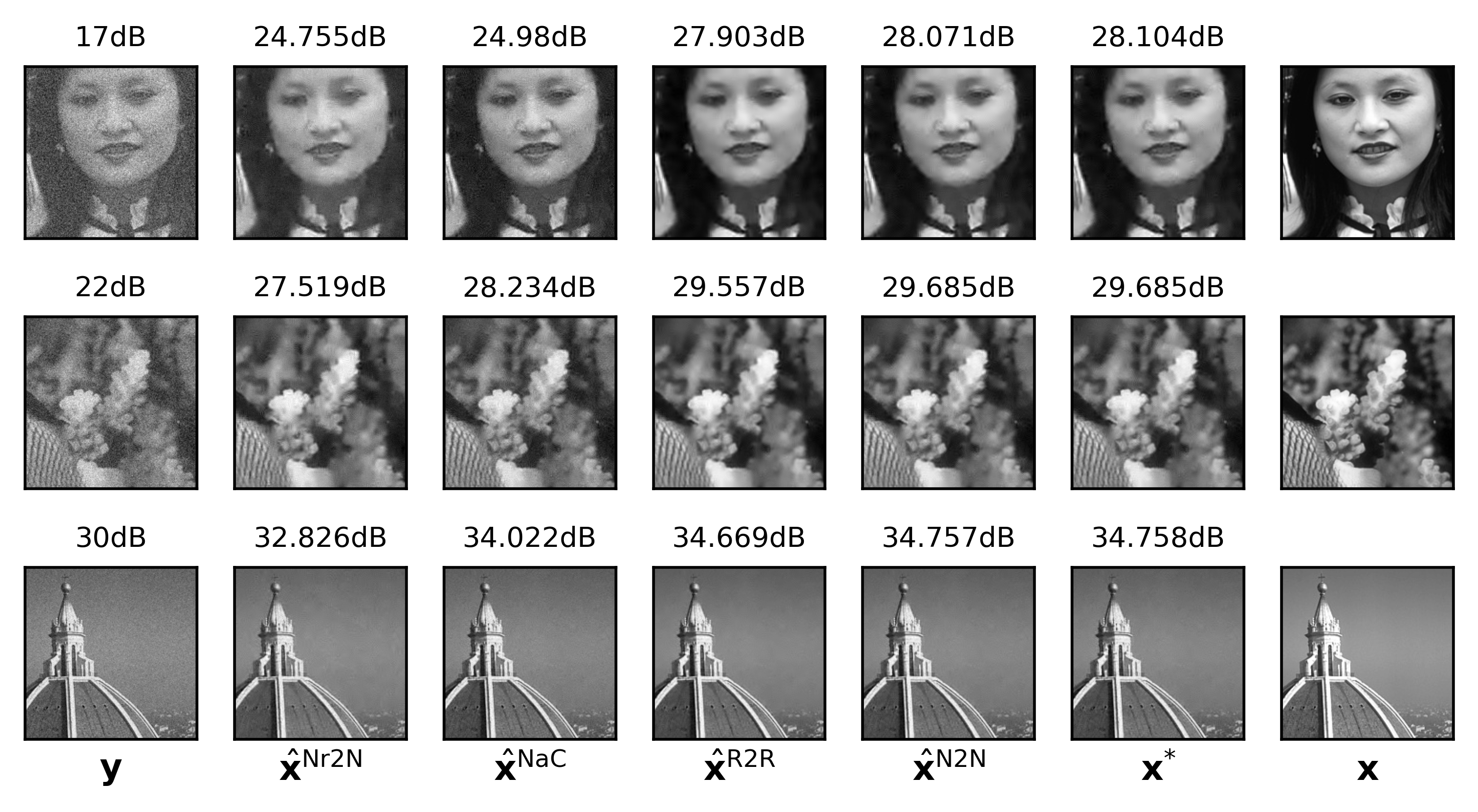
Figure 1: Exemple of denoising results. The upper scripts of $\mathbf{\hat{x}}$ refer to the corresponding method; $\mathbf{x}^{*}$ and $\mathbf{x}$ denote respectively the result for the supervised (gold standard) approach and the ground-truth.

II-C Use case: Denoising via Quantum Interactive Patches

We illustrate our method, without loss of generality, to a denoiser, denoted DeQuIP (Denoising via Quantum Interactive Patches) [3] which can handle various types of noise. It is based on two main concepts of quantum mechanics: (i) exploits the Schrödinger equation of quantum physics to construct an adaptive basis, which enables DeQuIP to deal with various noise models; (ii) treats the image as patches, and formalizes the self-similarity between neighbor patches through a term akin to quantum many-body interaction to efficiently preserve the local structures. Each patch behaves as a single-particle system, which interacts with other neighboring patches, thus the whole image acts as a many-body system. Under a potential ${\mathbf{V}}$, represented by the image pixel values [20], the adaptive basis vector ${\bm{\uppsi}}$ describes the characteristics of a virtual quantum particle with energy $E$, and satisfies the non-relativistic stationary Schrödinger equation, written as:

$$-\frac{\hbar^{2}}{2m}\nabla^{2}{\bm{\uppsi}}=-{\mathbf{V}}{\bm{\uppsi}}+E{\bm{\uppsi}},$$ (11)

with $\hbar$ being Planck’s constant, $m$ the particle mass, and $\nabla^{2}$ the Laplacian operator. The image-dependent basis is constructed from the wave solutions ${\bm{\uppsi_{i}}}$ of eq. (11) by plugging the noisy image $\mathbf{y}$ as the potential ${\mathbf{V}}$ of the system. These wave solutions are oscillating functions with a local frequency proportional to $\sqrt{(E-{\mathbf{V}})/(\hbar^{2}/2m)}$, thus the frequency is locally adapted to the image pixels’ values. The exact behavior of these basis vectors with respect to the potential is determined by the constant $\frac{\hbar^{2}}{2m}$, which is a parameter of DeQuIP. For a more detailed illustration of these oscillating wave vectors, we refer readers to [20, 21]. Finally, for denoising, the noisy image $\mathbf{y}$ is projected onto this adaptive basis, and the low-value coefficients are thresholded using a soft threshold:

$$\Upsilon_{c_{1},c_{2}}(x)=\left\{\begin{matrix}[l]0&\text{if }|\alpha|\leq c_{1}\\ \frac{c_{2}}{c_{2}-c_{1}}x-\frac{c_{1}c_{2}}{c_{2}-c_{1}}&\text{if }-c_{2}\leq x\leq-c_{1}\\ \frac{c_{2}}{c_{2}-c_{1}}x+\frac{c_{1}c_{2}}{c_{2}-c_{1}}&\text{if }c_{2}\geq x\geq c_{1}\\ 1&\text{elsewhere}\end{matrix}\right.$$

The second key idea of DeQuIP is the integration of quantum interaction theory to consider the image as overlapping patches, where each patch is a single-particle system that interacts with other patches [3]. The interaction between two patches $\mathbf{A}$ and $\mathbf{B}$ is defined as: ${\mathbf{I}}_{AB}=p\frac{|{\mathbf{A}}-{\mathbf{B}}|}{d(A,B)^{2}}$ with $p$ a parameter controlling the strength of the interaction term, and $d$ the euclidean pixel distances between the center of $\mathbf{A}$ and $\mathbf{B}$. This term is designed to promote local self-similarity, based on the hypothesis that neighboring patches in an image are likely to be more similar than distant ones.

Therefore, DeQuIP has $4$ parameters $\bm{\uptheta}=\{-\frac{\hbar^{2}}{2m},p,c_{1},c_{2}\}$ shared across patches.

III Experimental results

III-A Material & Data

Implementation is done on PyTorch 1.12.0. We used $180\times 180$ clean grayscale photographic images, extracted from the BSD400 dataset, as ground truth.

III-B Comparison of Denoised Images

The estimates $\hat{\mathbf{x}}^{\mathrm{N2N}}$, $\hat{\mathbf{x}}^{\mathrm{NaC}}$, $\hat{\mathbf{x}}^{\mathrm{Nr2N}}$, $\hat{\mathbf{x}}^{\mathrm{R2R}}$ and the gold standard $\mathbf{x}^{*}$ are compared in the zero-mean Gaussian noise case since it is the only case covered by the four proposed schemes. We report on Fig. 2 the average performance (measured by output PSNR) and standard deviation over 35 test images as a function of the input PSNR. Examples of noisy and denoised images are presented in Fig. 1. We see, both in metric and visually, that $\hat{\mathbf{x}}^{\mathrm{N2N}}$ and $\hat{\mathbf{x}}^{\mathrm{R2R}}$ achieve the gold standard performance $\mathbf{x}^{*}$. As expected given the assumptions it relies on, $\hat{\mathbf{x}}^{\mathrm{NaC}}$ yields better results when noise is low enough (i.e., high PSNR), but still underperforms. Finally, $\hat{\mathbf{x}}^{\mathrm{Nr2N}}$ does not perform as well as the other unsupervised methods.

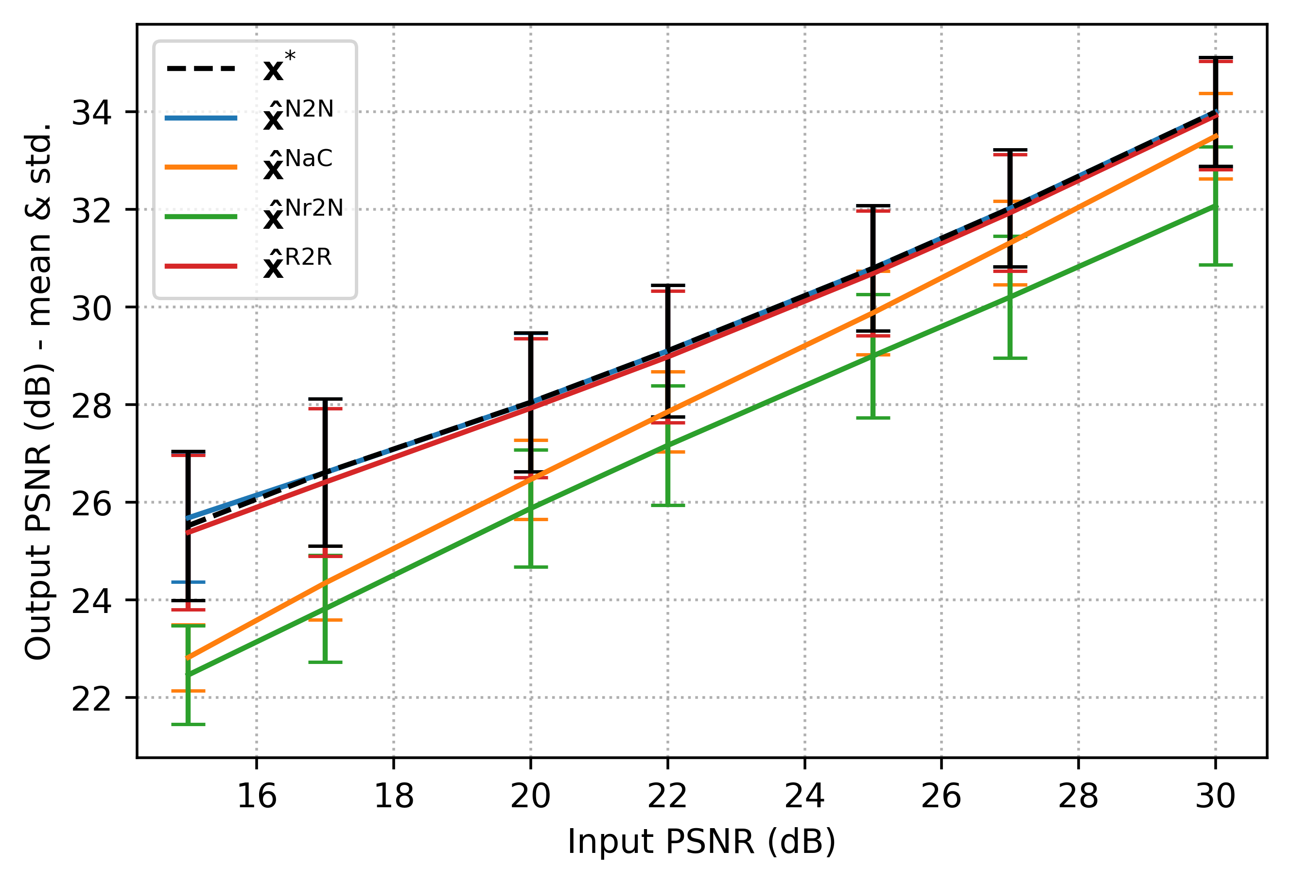
Figure 2: Comparison of the proposed strategies with the gold standard $\mathbf{x}^{*}$. The average performance and standard deviation is computed over 35 test images.

III-C Poisson Noise Denoising

As DeQuIP can deal with various noise models, we present in Fig. 3 Poisson noise denoising results, where we can observe that $\hat{\mathbf{x}}^{\mathrm{N2N}}$ is similar to $\mathbf{x}^{*}$. We used $\widehat{\mathcal{C}}^{\mathrm{N2N}}$ because of its performances, and its capacity to handle Poisson noise.

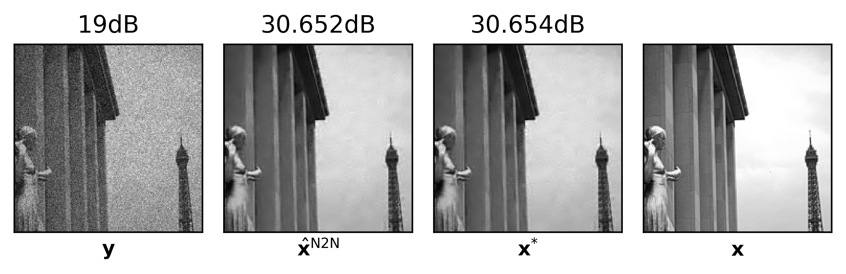
Figure 3: Poisson noise denoising.

IV Conclusion

We have proposed a method for the automatic tuning of denoising algorithm parameters, leveraging only the noisy measurements targeted for enhancement. Specially, we introduced several cost functions and inference schemes, two of which yielded results comparable to those obtained with ground truth-tuned parameters.
However, our method comes with certain limitations. The first one arises when only a single noisy image is available, requiring the noise to follow a zero-mean Gaussian distribution. For other types of noise, two independent noisy versions are needed. The second limitation is the need to resolve an optimization problem that involves differentiating the denoising algorithm with respect to its parameters. Although this can be achieved using a simple backpropagation, it can be computationally expensive.
Moving forward, there are potential avenues for exploration. For algorithms $A$ that cannot replicate the identity function, exploring unsupervised losses inspired by Noise2Self [22] and [23] could be fruitful, given their advantage of using a single noise realization $\mathbf{y}$ without renoising it. Another idea worth exploring is the extension of our method to other inverse problems such as image deblurring or super-resolution, possibly building on [24, 25].

References

- [1] Kostadin Dabov, Alessandro Foi, Vladimir Katkovnik and Karen Egiazarian “Image Denoising by Sparse 3-D Transform-Domain Collaborative Filtering” In IEEE Transactions on Image Processing 16.8, 2007, pp. 2080–2095 DOI: 10.1109/TIP.2007.901238
- [2] Ivan Selesnick “Total Variation Denoising Via the Moreau Envelope” In IEEE Signal Processing Letters 24.2, 2017, pp. 216–220 DOI: 10.1109/LSP.2017.2647948
- [3] Sayantan Dutta, Adrian Basarab, Bertrand Georgeot and Denis Kouamé “A Novel Image Denoising Algorithm Using Concepts of Quantum Many-Body Theory” In Signal Processing 201 Elsevier BV, 2022, pp. 108690 DOI: 10.1016/j.sigpro.2022.108690
- [4] Luca Calatroni et al. “Bilevel approaches for learning of variational imaging models” In Variational Methods: In Imaging and Geometric Control 18.252 Walter de Gruyter GmbH, 2017, pp. 2 DOI: 10.1515/9783110430394-008
- [5] Pascal Nguyen, Emmanuel Soubies and Caroline Chaux “MAP-informed Unrolled Algorithms for Hyper-parameter Estimation” In International Conference on Image Processing IEEE, 2023
- [6] Babak Maboudi Afkham, Julianne Chung and Matthias Chung “Learning regularization parameters of inverse problems via deep neural networks” In Inverse Problems 37.10 IOP Publishing, 2021, pp. 105017 DOI: 10.1088/1361-6420/ac245d
- [7] Andreas Kofler et al. “Learning Regularization Parameter-Maps for Variational Image Reconstruction using Deep Neural Networks and Algorithm Unrolling” In arXiv Preprint, Jan. 2023 DOI: 10.48550/arXiv.2104.06594
- [8] Jaakko Lehtinen et al. “Noise2Noise: Learning Image Restoration without Clean Data” In International Conference on Machine Learning PMLR, Mar. 2018 DOI: 10.48550/arXiv.1803.04189
- [9] Jun Xu et al. “Noisy-as-Clean: Learning Self-Supervised Denoising From Corrupted Image” In IEEE Transactions on Image Processing 29, 2020, pp. 9316–9329 DOI: 10.1109/TIP.2020.3026622
- [10] Nick Moran, Dan Schmidt, Yu Zhong and Patrick Coady “Noisier2Noise: Learning to Denoise from Unpaired Noisy Data” In Conference on Computer Vision and Pattern Recognition IEEE/CVF, Oct. 2019 DOI: 10.48550/arxiv.1910.11908
- [11] Tongyao Pang, Huan Zheng, Yuhui Quan and Hui Ji “Recorrupted-to-Recorrupted: Unsupervised Deep Learning for Image Denoising” In Conference on Computer Vision and Pattern Recognition IEEE/CVF, 2021, pp. 2043–2052 DOI: 10.1109/CVPR46437.2021.00208
- [12] G. H, Golub, Heath M and Wahba G “Generalized cross-validation as a method for choosing a good ridge parameter,” In Technometrics, 21.12, 1979 DOI: 10.1109/TIP.2010.2052820
- [13] Charles M Stein “Estimation of the mean of a multivariate normal distribution” In The annals of Statistics JSTOR, 1981, pp. 1135–1151
- [14] C. Deledalle, S. Vaiter, J.and Fadili and G. Peyré “Stein Unbiased GrAdient estimator of the Risk (SUGAR) for Multiple Parameter Selection” In SIAM Journal on Imaging Sciences 7.2, 2014, pp. 2448–2487
- [15] S. Ramani, T. Blu and M. Unser “Monte-Carlo Sure: A Black-Box Optimization of Regularization Parameters for General Denoising Algorithms” In IEEE Transactions on Image Processing 17.9, 2008, pp. 1540–1554 DOI: 10.1109/TIP.2008.2001404
- [16] Xiang Zhu and Peyman Milanfar “Automatic Parameter Selection for Denoising Algorithms Using a No-Reference Measure of Image Content” In IEEE Transactions on Image Processing 19.12, 2010, pp. 3116–3132 DOI: 10.1109/TIP.2010.2052820
- [17] Xiangfei Kong and Qingxiong Yang “No-Reference Image Quality Assessment for Image Auto-Denoising” In International Journal of Computer Vision 126.5, 2018, pp. 537–549 DOI: 10.1007/s11263-017-1054-2
- [18] Xue Ying “An Overview of Overfitting and its Solutions” In Journal of Physics: Conference Series 1168, 2019, pp. 022022 DOI: 10.1088/1742-6596/1168/2/022022
- [19] Dmitry Ulyanov, Andrea Vedaldi and Victor Lempitsky “Deep Image Prior” In Conference on Computer Vision and Pattern Recognition IEEE/CVF, 2018, pp. 1867–1888 DOI: 10.1007/s11263-020-01303-4
- [20] S. Dutta, A. Basarab, B. Georgeot and D. Kouamé “Quantum Mechanics-Based Signal and Image Representation: Application to Denoising” In IEEE Open Journal of Signal Processing 2, 2021, pp. 190–206 DOI: 10.1109/OJSP.2021.3067507
- [21] S. Dutta, A. Basarab, B. Georgeot and D. Kouamé “Image Denoising Inspired by Quantum Many-Body physics” In 2021 IEEE International Conference on Image Processing (ICIP), 2021, pp. 1619–1623 DOI: 10.1109/ICIP42928.2021.9506794
- [22] Alexander Krull, Tim-Oliver Buchholz and Florian Jug “Noise2void-learning denoising from single noisy images” In Conference on Computer Vision and Pattern Recognition IEEE/CVF, 2019, pp. 2129–2137 DOI: 10.48550/arXiv.1811.10980
- [23] Joshua Batson and Loic Royer “Noise2self: Blind denoising by self-supervision” In International Conference on Machine Learning, 2019, pp. 524–533 PMLR DOI: 0.48550/arXiv.1901.11365
- [24] Zhihao Xia and Ayan Chakrabarti “Training Image Estimators without Image Ground Truth” In Advances in Neural Information Processing Systems 32 Curran Associates, Inc., 2019 URL: https://proceedings.neurips.cc/paper_files/paper/2019/file/0ed9422357395a0d4879191c66f4faa2-Paper.pdf
- [25] Julián Tachella, Dongdong Chen and Mike Davies “Unsupervised Learning From Incomplete Measurements for Inverse Problems” In Proceedings of the 36th Conference on Neural Information Processing Systems, 2022