Abstract

Flux attachment provides a powerful conceptual framework for understanding certain forms of topological order, including most notably the fractional quantum Hall effect. Despite its ubiquitous use as a theoretical tool, directly realizing flux attachment in a microscopic setting remains an open challenge. Here, we propose a simple approach to realizing flux attachment in a periodically-driven (Floquet) system of either spins or hard-core bosons. We demonstrate that such a system naturally realizes correlated hopping interactions and provides a sharp connection between such interactions and flux attachment. Starting with a simple, nearest-neighbor, free boson model, we find evidence—from both a coupled wire analysis and large-scale density matrix renormalization group simulations—that Floquet flux attachment stabilizes the bosonic integer quantum Hall state at $1/4$ filling (on a square lattice), and the Halperin-221 fractional quantum Hall state at $1/6$ filling (on a honeycomb lattice). At $1/2$ filling on the square lattice, time-reversal symmetry is instead spontaneously broken and bosonic integer quantum Hall states with opposite Hall conductances are degenerate. Finally, we propose an optical-lattice-based implementation of our model on a square lattice and discuss prospects for adiabatic preparation as well as effects of Floquet heating.

Unlike more conventional states, topological phases cannot be identified by their pattern of symmetry breaking, but rather, by the underlying structure of their entanglement Chen et al. (2010). Despite tremendous recent advances in the theoretical classification Chen et al. (2013); Lu and Vishwanath (2012) of both intrinsic topological order Tsui et al. (1982); Laughlin (1983) and symmetry-protected topological (SPT) order Chen et al. (2013); Haldane (1983); Pollmann et al. (2010); Vishwanath and Senthil (2013), there are, as yet, few guiding principles for obtaining simple realizations of strongly-interacting topological phases.

From a conceptual viewpoint, one such principle, which underlies our understanding of the fractional quantum Hall effect , is the notion of flux attachment Girvin and MacDonald (1987); Zhang et al. (1989); Jain (1989); Zhang (1992); the conventional picture states that Coulomb repulsion has the net effect of attaching an even number of magnetic flux quanta to every electron. Such composite objects obey the Pauli principle and feel a smaller effective magnetic field (in fact, one which mimics that of an integer quantum Hall effect); to this end, flux attachment provides a unified description for, and explains the similarity between, the experimental results for the integer and fractional cases.

A considerable amount of recent attention has focused on correlated hopping Greschner et al. (2014a); Di Liberto et al. (2014); Hudomal et al. (2020); Lienhard et al. (2020); Chu et al. (2023) of the form, $H=(2n_{k}^{b}-1)a_{j}^{\dagger}a_{i}$ [Fig. 1(a,b)], in part because it provides a natural framework for implementing flux attachment He et al. (2015a); Fuji et al. (2016); Liu et al. (2019). In particular, within this Hamiltonian setting, the $a$-particles naturally see the density of $b$-particles as flux since, $e^{i\pi n^{b}_{k}}=(1-2n_{k}^{b})$. In addition to enabling a more direct mapping between analytic predictions and micro-

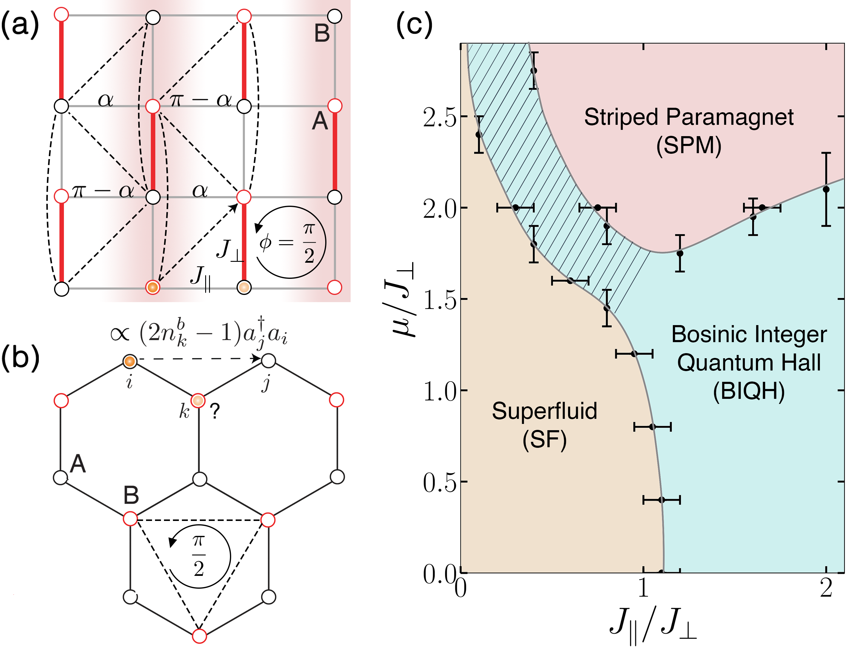
Figure 1: (a) Schematic depiction of our square-lattice, correlated-hopping model for two species of hard-core bosons (residing on the A and B sublattice). The background flux of the nearest-neighbor Floquet-driven Hamiltonian is $\phi$ per square plaquette, leading to an effective Hamiltonian with staggered flux $\pi/2\pm\phi$ per triangular loops shown with dotted lines. The added flux $\alpha$ breaks the time reversal symmetry of the effective Hamiltonian. The striped chemical potential (red shading) $V=\pm\mu$ facilitates adiabatic preparation. (b) Analogous model for a honeycomb lattice, where the background flux is $\pi/2$ per triangular plaquette ($\pi$ per hexagon). (C) Phase diagram of the square lattice model with $\phi=\pi/2$ at half filling computed via iDMRG on a cylinder of width $L=10$ lattice sites.The hashed region appears to be smoothly connected to the BIQH phase (see text). The error bars originate from the resolution of the numerics and the flow of the transition with bond dimension.

scopic models, such correlated-hopping Hamiltonians have also been shown to exhibit (fractional) Chern insulators at anomalously large background fluxes He et al. (2015a); understanding the interplay between topology and lattice-symmetries in this high-flux-regime is the subject of active investigation Regnault and Bernevig (2011); Murthy and Shankar (2012); Zhao et al. (2021); Chen et al. (2012); Liu and Bergholtz (2022); Lin et al. (2023).

Despite seminal advances  Liu et al. (2019); Greschner et al. (2014b, a), owing to the multi-body nature of the interactions, it remains an open challenge to directly implement correlated hopping. In this Letter, we propose and analyze a method to realize correlated hopping in a periodically-driven (Floquet) system of spins or hard-core bosonic particles. Our main results are threefold. First, we analytically illustrate the emergence of correlated hopping from the periodic modulation Dunlap and Kenkre (1986); Aidelsburger et al. (2011); Struck et al. (2012); Jiménez-García et al. (2012); Jotzu et al. (2014) of a simple hard-core boson model. We utilize a perturbative coupled-wire construction to explore the existence of topological phases in the resulting many-body Hamiltonian. Second, guided by this analysis, we perform large-scale density matrix renormalization group (DMRG) simulations Hauschild and Pollmann (2018), which reveal the existence of both a bosonic integer quantum Hall (BIQH) phase on the square lattice He et al. (2015a); Fuji et al. (2016); Liu et al. (2019); Miao et al. (2022), and a bosonic fractional quantum hall (BFQH) phase on the honeycomb lattice Fuji et al. (2016); Léonard et al. (2022). Surprisingly, we also discover a regime where the Hamiltonian is explicitly time-reversal invariant, and yet, hosts a robust BIQH ground state; in this regime, we find that BIQH states with either sign of the Hall conductance are simultaneously stable He et al. (2015b).

Finally, motivated by the possibility of adiabatically preparing the BIQH in cold atomic systems Barkeshli et al. (2015); Motruk and Pollmann (2017), we explore the surrounding phase diagram as a function of two natural experimental control parameters: the anisotropy of the hopping strengths, and an overlaid striped chemical potential. We provide a specific experimental blueprint for realizing our protocol in a lattice gas of ultracold bosonic atoms Goldman et al. (2014); Dalibard (2015); Zhai (2015); Goldman et al. (2016); Cooper et al. (2019); we emphasize that our protocol can also be implemented in Rydberg tweezer arrays where synthetic gauge fields arise from either dipolar exchange interactions Yao et al. (2013); Cesa and Martin (2013); Lienhard et al. (2020) or local dressing fields Wu et al. (2022); Celi et al. (2014). In addition to providing a microscopic route to both realizing and understanding flux attachment, our approach opens the door to a more general framework for defect-particle binding and the simulation of exotic phases and phase transitions Senthil et al. (2004); Senthil and Levin (2013); Xu and Senthil (2013); Liu et al. (2014).

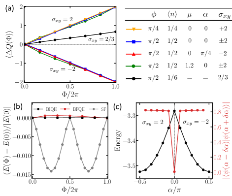
Figure 2: (a) Charge pumping under flux insertion provides numerical evidence for the BIQH state on the square lattice at various parameters, and the Halperin-221 fractional quantum Hall state on the isotropic honeycomb lattice (last row of the table). $J_{\parallel}/J_{\perp}=2$ for all the plotted BIQH states. The BIQH states were observed on various cylinder widths, $L=6,8,10$ lattice sites and the BFQH state on a cylinder of width $L=12$ sites. (b) The negligible change in the ground state energy under flux insertion in the BFQH and half-filled BIQH phases, contrasted with that in the superfluid phase on the square lattice at $J_{\parallel}/J_{\perp}=0.4$. The superfluid energy has periodicity $\pi$ under flux insertion because for odd sublattice cylinder widths ($L/2$), the ground states for periodic and antiperiodic boundary conditions are exactly degenerate. (c) Energy and Fidelity (wavefunction overlap) as a function of time-reversal symmetry-breaking parameter $\alpha$, showing a first order phase transition between the two BIQH phases with $\sigma_{xy}=\pm 2$ on the square lattice, with $\phi=\pi/2,\langle n\rangle=1/2$, $J_{\parallel}/J_{\perp}=2$, and $\delta\alpha=\pi/24$.

Floquet Flux Attachment—Let us start by demonstrating how a periodically-driven system of free hard-core bosons can generate correlated hopping. Suppose two identical species of bosons reside separately on the sublattices, $A$ and $B$, of a bipartite lattice [Fig. 1(a,b)]. Consider the Hamiltonian

$$H(t)=\sum_{\langle ik\rangle}[J_{ik}\cos(\Omega t+\theta_{ik})e^{i{\mathcal{B}}_{ik}}a^{\dagger}_{i}b_{k}+h.c.],$$ (1)

where $a$ ($b$) is the annihilation operator for a hard-core boson on sublattice $A$ ($B$), ${\mathcal{B}}_{ik}$ captures a background flux, $\theta_{ik}$ are bond-dependent constants, and the nearest-neighbor hopping amplitudes are periodically modulated at frequency $\Omega$. One can factor out the periodic drive, $H(t)=e^{i\Omega t}H_{1}+e^{-i\Omega t}H_{-1}$, where $H_{1}=\sum_{\langle ik\rangle}J_{ik}e^{i\theta_{ik}}[e^{i{\mathcal{B}}_{ik}}a^{\dagger}_{i}b_{k}+h.c.]$ and $H_{-1}=\sum_{\langle ik\rangle}J_{ik}e^{-i\theta_{ik}}[e^{i{\mathcal{B}}_{ik}}a^{\dagger}_{i}b_{k}+h.c.]$. For large driving frequencies, the Hamiltonian can be expanded in powers of $1/\Omega$ using a Floquet-Magnus expansion; the leading order term is given by Goldman and Dalibard (2014):

$$H_{\rm eff}=\frac{1}{\Omega}[H_{1},H_{-1}]$$

$$=\frac{2}{\Omega}\sum_{ij;k}J_{ik}J_{kj}\sin(\theta_{ik}-\theta_{kj})\left[ie^{i{\mathcal{B}}_{ij}}(2n_{k}^{b}-1)a^{\dagger}_{i}a_{j}+h.c.\right]$$

$$+\frac{2}{\Omega}\sum_{kl;i}J_{ki}J_{il}\sin(\theta_{ki}-\theta_{il})\left[ie^{i{\mathcal{B}}_{kl}}(2n_{i}^{a}-1)b^{\dagger}_{k}b_{l}+h.c.\right].$$ (2)

Crucially, $H_{\rm eff}$ exhibits correlated hopping—as the $a$-bosons hop on the $A$ sublattice, they acquire a phase which depends on the occupation of the intervening $B$-lattice site ($n_{k}^{b}=b^{\dagger}_{k}b_{k}=0,1$), and vice versa. This effective static Hamiltonian is prethermal and describes the system for exponentially long times $\sim e^{\Omega/J}$, before drive-induced Floquet heating occurs Bukov et al. (2016); Kuwahara et al. (2016); Mori et al. (2016); Abanin et al. (2017); Weidinger and Knap (2017); Machado et al. (2019).

Bosonic Integer Quantum Hall Phase—Consider Eq. (S0.Ex1) on the square lattice, where the hopping amplitudes along the horizontal and vertical directions are given by $J_{\parallel}$ and $J_{\perp}$, respectively [Fig. 1(a)]. Using a coupled-wire construction, we investigate the existence of interesting quantum Hall states Fuji et al. (2016); Fuji and Furusaki (2019). To facilitate this approach, we choose $\theta_{ik}=\pi/2$ on the thick red bonds depicted in Fig. 1(a), while $\theta_{ik}=0$ otherwise. The consequence of this choice for $H_{\textrm{eff}}$ is that bosons can only hop to their next-nearest neighbors vertically and diagonally, with coupling strengths proportional to $J_{\perp}^{2}$ and $J_{\perp}J_{\parallel}$, respectively. Thus, when the ratio $J_{\parallel}/J_{\perp}$ vanishes, the bosons cannot hop between vertical chains. A simple Jordan-Wigner transformation reveals that the chains decouple into gapless Luttinger liquids. Turning on the diagonal hopping between chains gaps out the bulk degrees of freedom, but a perturbative analysis reveals that gapless modes can survive at the edge, suggesting a quantum Hall state SM . In particular, we find that for a system with boson density $\langle n\rangle$ per site and background flux $\phi=\sum_{ij}{\mathcal{B}}_{ij}=\pi(2p+2q+1)\langle n\rangle$ per plaquette ($p,q\in\mathbb{Z}$), it is possible to realize a Halperin state, where the commutation relations between the gapless modes are described by the Chern-Simons $K$-matrix: $K=\begin{pmatrix}2p&&2q+1\\ 2q+1&&2p\end{pmatrix}$ Wen (1995); Lu and Vishwanath (2012).

The simplest possible such state is the BIQH, a symmetry-protected topological phase of matter characterized by $K=\begin{pmatrix}0&&1\\ 1&&0\end{pmatrix}$. Guided by the above analysis, we use iDMRG to compute the ground state at filling factor $\nu=2\pi\langle n\rangle/\phi=2$, where $\phi=\pi/4$ and $\langle n\rangle=1/4$, in the hope of observing a BIQH state. We choose a large value of the ratio $J_{\parallel}/J_{\perp}=2$, such that the system should presumably be deep in this topological phase. The system is wrapped around an infinitely long cylinder with the vertical ($J_{\perp}$) and horizontal ($J_{\parallel}$) hoppings in the wrapping and infinite direction respectively, although we confirm that the choice of wrapping direction has no qualitative effect SM .

A tell-tale signature of the BIQH phase is its Hall conductance $\sigma_{xy}$, which is always quantized to an even integer. Within iDMRG, in order to compute $\sigma_{xy}$ Laughlin (1981), we thread $2\pi$ flux through the cylinder and measure the resulting charge pumping He et al. (2014); Grushin et al. (2015). As shown in Fig. 2(a), the charge pumped increases linearly as a function of the inserted flux, $\Delta Q\equiv\frac{\Phi}{2\pi}\sigma_{xy}=\frac{\Phi}{\pi}$, providing evidence that the ground state of the system is a BIQH state with a quantized Hall conductance, $\sigma_{xy}=2$.

Moreover, the ground state energy remains nearly constant under flux insertion, indicating that the system is gapped [Fig. 2(b)]. The large entanglement entropy and short correlation length provide further evidence that the ground state is indeed a gapped, entangled liquid [Figs. 3(a)]. Our numerics suggest that this BIQH state is stable for any $J_{\parallel}/J_{\perp}\gtrsim 0.3$ SM .

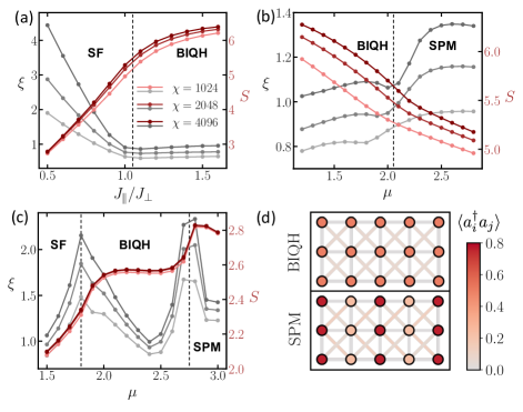
Figure 3: Phase transitions out of the spontaneous time-reversal symmetry-breaking BIQH phase: correlation length $\xi$ along the cylinder direction and entanglement entropy $S$: (a) at fixed $\mu=0$, showing a phase transition from a superfluid to BIQH with increasing $J_{\parallel}/J_{\perp}$, (b) at fixed $J_{\parallel}/J_{\perp}=2.0$, showing a phase transition from BIQH to a striped paramagnetic phase with increasing $\mu$, (c) at fixed $J_{\parallel}/J_{\perp}=0.4$, showing the various phase transitions from a superfluid to the striped paramagnetic phase with increasing $\mu$. The intervening phase appears to be smoothly connected to the BIQH. (d) Density and nearest-neighbor correlations for the BIQH at $J_{\parallel}/J_{\perp}=2.0,\mu=0$ and the SPM at $J_{\parallel}/J_{\perp}=2.0,\mu=2.4$. All the data is acquired on a cylinder of width $L=10$ lattice sites.

Bosonic Fractional Quantum Hall—Our coupled wire analysis suggests that even more exotic states can be realized. For example, choosing $p=1,q=0$ yields the 221-Halperin state He et al. (2015a); Fuji et al. (2016), which is topologically ordered, exhibits a fractional Hall conductance $\sigma_{xy}=2/3$ and supports chiral edge modes, unlike the BIQH state. Unfortunately, we were unable to stabilize such a state on the square lattice. However, a similar coupled wire analysis on the honeycomb lattice [Fig 1(b)] predicts the emergence of a 221-Halperin ground state for the parameters: $J_{ik}=J$, $\langle n\rangle=1/6$, $\theta_{ik}=0,2\pi/3,4\pi/3$ and a background flux of $\pi/2$ per triangular plaquette  He et al. (2015a); Fuji et al. (2016). To investigate this prediction, we again perform iDMRG and measure charge pumping as a function of flux insertion. As depicted in Fig. 2(a), we indeed observe the expected $\sigma_{xy}=2/3$. We note that the ground state energy exhibits a weak dispersion as a function of flux insertion [Fig. 2(b)], albeit significantly smaller than the superfluid that we will soon discuss.

Spontaneous Time-Reversal Symmetry Breaking—A naive interpretation of our coupled wire analysis might seem to suggest that a BIQH phase should also be stable for even larger external flux $\phi=\pi/2$ and filling $\langle n\rangle=1/2$. However, at these parameter values, the coupled wire analysis is unable to distinguish between the two different BIQH phases with Hall conductance $\sigma_{xy}=\pm 2$. This is because the effective correlated-hopping model [Eq. (S0.Ex1)] is time-reversal invariant for external flux $\phi=\pi/2$—an emergent symmetry which is broken by higher order terms in the Floquet-Magnus expansion.

Due to this emergent time-reversal symmetry, it is natural to assume that the ground state for the effective model must be time-reversal invariant. However, iDMRG instead finds two degenerate ground states which break time-reversal symmetry with Hall conductance $\sigma_{xy}=\pm 2$ [Fig. 2(a)]. This degeneracy can be lifted by applying an additional staggered flux, $\pm\alpha$, per next-nearest neighbor triangular plaquette [Fig. 1(a)]. The original, time-reversal invariant point at $\alpha=0$ can then be reinterpreted as the phase transition point separating the two BIQH phases. If the phase transition is continuous, one expects a time-reversal invariant critical ground state He et al. (2015a). Instead, we find strong evidence from both the energy and wavefunction overlap [Fig. 2(c)] that the transition is first order, with concurrent spontaneous time-reversal symmetry-breaking at $\alpha=0$.

Interestingly, this model realizes a BIQH state at an unusually large background flux, $\phi=\pi/2$. Indeed, other models which host the BIQH state, such as the bosonic Harper-Hofstadter model, generally require a smaller flux, which is closer to the continuum limit Sterdyniak et al. (2015); He et al. (2017). In contrast, constructing a quantum Hall state by exploiting correlated-hopping to directly drive flux attachment allows for the realization of the BIQH state in a more lattice-dominated regime.

Phase diagram for adiabatic preparation—In order to explore the possible adiabatic preparation of this spontaneous time-reversal symmetry-breaking BIQH state, we identify two natural tuning parameters, which can drive the system into nearby phases exhibiting lower entanglement. In particular, we construct the phase diagram on the square lattice surrounding the BIQH state as a function of: (i) the hopping anisotropy $J_{\parallel}/J_{\perp}$, and (ii) a striped chemical potential, $V=\pm\mu$ [Fig. 1(a)].

Let us begin by setting $\mu=0$ and varying the anisotropy. As illustrated in Fig. 3(a), the system undergoes a phase transition out of the BIQH state as $J_{\parallel}/J_{\perp}$ is decreased. For $J_{\parallel}/J_{\perp}\lesssim 1$, we observe three features indicative of a superfluid phase: (i) a sharp decrease of the entanglement entropy, (ii) a rapid growth of the correlation length with bond dimension and (iii) sharp peaks in the structure factor SM . In addition, for a superfluid, flux insertion is expected to frustrate the phase coherence and lead to spectral flow of the ground state energy, as depicted in Fig. 2(b). Interestingly, our coupled wire analysis suggests that the BIQH phase should be stable for any non-vanishing $J_{\parallel}$, suggesting the possibility that the superfluid region in the phase diagram could vanish in the thermodynamic limit; the observed superfluid is perhaps stabilized by the energy gap present in our finite-width cylinder geometry.

Let us now turn on the chemical potential, $\mu$ [Fig. 1(a)]. By doing so, we explicitly break translation symmetry along the cylinder axis, while leaving it intact along the perpendicular direction. At large $\mu$, one expects the system to be in a paramagnetic state which conforms to this externally-imposed symmetry breaking. This is precisely what is observed upon increasing $\mu$ at fixed $J_{\parallel}/J_{\perp}=2$. As depicted in Fig. 3(b), the system remains in the BIQH phase for small values of the chemical potential, and then transitions, at $\mu_{\textrm{c}}=2.0\pm 0.1$ into a striped paramagnet SM , a phase easy to access experimentally. Intriguingly it appears that there is no direct transition from the striped paramagnet to the superfluid phase, and instead there is always an intervening phase [Fig. 3(c)]. This phase appears to be smoothly connected to the BIQH phase, although we cannot verify integer charge pumping in the hashed region [Fig. 1(c)] due to its proximity to several phase transitions.

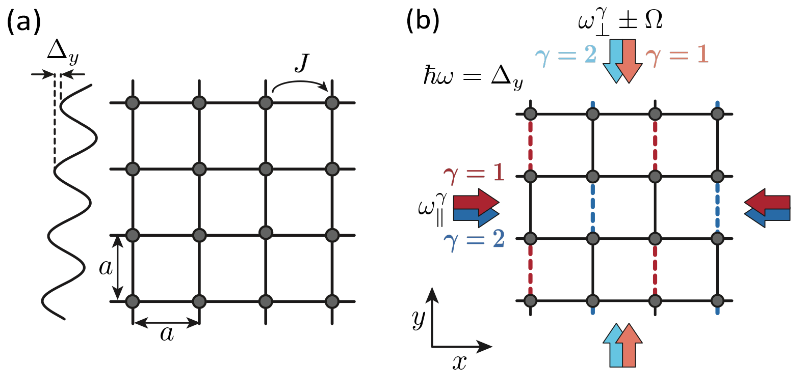
Figure 4: Schematic depiction of the proposed experimental setup. (a) We focus on ⁸⁷Rb in a square optical lattice. The bosonic hopping $J$ is suppressed by an overlaid linear potential $\Delta_{y}$. (b) The hopping is restored by laser assisted tunneling. Depicted are two of the four lasers used (red/blue arrows). These allow for Floquet modulation of the correspondingly colored bonds, as well as control of the background flux.

Experimental realization—Motivated by recent advances in the implementation and characterization of topological phases in cold atomic systems Dalibard et al. (2011); Goldman et al. (2014); Jotzu et al. (2014); Aidelsburger et al. (2015a); Tai et al. (2017); Barbiero et al. (2019); Léonard et al. (2022); Impertro et al. (2023), we propose an experimental protocol to directly realize our correlated hopping model. In particular, we envision realizing Eq. (1) via laser-assisted tunneling of neutral atoms in a two-dimensional optical lattice Jaksch and Zoller (2003); Aidelsburger et al. (2015b). To be specific, we consider ⁸⁷Rb and focus on a square lattice geometry where Harper-Hofstadter models have already been experimentally investigated Miyake et al. (2013); Aidelsburger et al. (2013, 2015a); Léonard et al. (2022). In the presence of a linear potential, $\Delta_{y}$, along the $y$ axis [Fig. 4(a)], the system is described by the following bosonic tight-binding Hamiltonian:

$$H_{0}= -J\sum_{m,n}\left(\hat{a}^{\dagger}_{m+1,n}\hat{a}_{m,n}+\hat{a}^{\dagger}_{m,n+1}\hat{a}_{m,n}+\text{h.c.}\right)$$

$$+\sum_{m,n}n\Delta_{y}\hat{n}_{m,n},$$ (3)

where $m$ ($n$) is the lattice site index along $x$ ($y$). For $\Delta_{y}\gg J$, tunneling is suppressed along the $y$-axis, while atoms are free to tunnel along the $x$ direction.

In order to restore resonant tunneling and to realize the background flux $\phi$ [Fig. 1(a)], we employ a resonant Floquet modulation scheme. Note that this Floquet modulation is used to realize $H_{\textrm{eff}}$ from $H_{0}$ and is distinct from the Floquet flux attachment described by Eq. (S0.Ex1). Choosing a set of four independent pairs of laser beams, labeled as $\gamma=\{1,2,3,4\}$ further enables us to realize the bond-dependent phases $\theta_{ik}$. For simplicity, only two pairs of beams are shown in Fig. 4(b). Let us illustrate the resonant modulation technique by focusing on the interference generated by a single pair. The two beams [e.g. $\gamma=1$ in Fig. 4(b)] are aligned along the $x$ and $y$ axes; both are vertically-polarized and retro-reflected, with wave vectors chosen to be $|\mathbf{k}_{\parallel}|\simeq|\mathbf{k}_{\perp}|=k=\frac{\pi}{2a}$, where $a$ is the lattice constant. This generates a time-dependent interference pattern that can be adjusted relative to the underlying square lattice in order to selectively modulate the colored bonds [Fig. 4(b)]. The laser beams along $y$ have two frequency components $\omega^{\gamma}_{\perp}\pm\Omega$ and the ones along $x$ have a single frequency component at $\omega^{\gamma}_{\parallel}$; crucially, the energy difference between the two beams, $\omega^{\gamma}_{\perp}-\omega^{\gamma}_{\parallel}=\omega=\Delta_{y}/\hbar$, is resonant with the potential energy difference between neighboring sites.

Up to constant terms, the spatially-varying, time-dependent potential resulting from each pair of laser beams can be expressed as:

$$V^{\gamma}(t)= V_{0}\cos(\omega t)\cos\left(\Omega t+\theta^{\gamma}_{0}\right)$$

$$\cos\left(m\frac{\pi}{2}+\varphi^{\gamma}_{x}\right)\cos\left(n\frac{\pi}{2}+\varphi^{\gamma}_{y}\right),$$ (4)

where $V_{0}$ is the strength of the potential and $\theta_{0}$ corresponds to the phase of the two sidebands at $\omega_{\perp}^{\gamma}\pm\Omega$. We specify the following phases for the four distinct pairs of laser-assisted tunneling beams: $\left(\varphi^{\gamma}_{x},\varphi^{\gamma}_{y}\right)=\{(0,\pi/4),(\pi/2,-\pi/4),(\pi,3\pi/4),(\pi/2,\pi/4)\}$. This allows us to modulate all of the vertical bonds in the lattice, while maintaining addressability of the phase $\theta_{0}$.

In the high-frequency limit, $\omega\gg J/\hbar$, $\Omega$, and for moderate modulation amplitudes $V_{0}\lesssim\hbar\omega$, the lowest-order Floquet Hamiltonian of the driven system, $H(t)=H_{0}+\sum_{\gamma}V^{\gamma}(t)$, can be expressed as:

$$H_{\textrm{F}}=-\sum_{m,n,\gamma}[J_{\text{eff}}\cos\left(\Omega t+\theta^{\gamma}_{0}\right)a^{\dagger}_{m,n}a_{m,n+1}\cos(m\frac{\pi}{2}+\varphi_{x}^{\gamma})$$

$$\hskip 38.0pt\sin(n\frac{\pi}{2}+\frac{\pi}{4}+\varphi_{y}^{\gamma})+Ja^{\dagger}_{m,n}a_{m+1,n}+\text{h.c.}],$$ (5)

where $J_{\text{eff}}=J\frac{V_{0}}{\sqrt{2}\Delta_{y}}$. This Hamiltonian realizes a staggered background flux. In order to achieve a homogeneous flux as well as amplitude modulation of the horizontal bonds, we add a staggered potential $\Delta_{m}=(-1)^{m}\Delta_{x}/2$ along the $x$ axis, and restore resonant tunneling via an additional pair of running laser beams Aidelsburger et al. (2015a).

To ensure that the leading-order approximations of both the laser Floquet modulation and the Floquet flux attachment are valid, the system must satisfy a hierarchy of energy scales: $\omega\gg J/\hbar$, $\Omega$ and $\Omega\gg J_{\text{eff}}/\hbar$. For ⁸⁷Rb, the following set of parameters satisfying these criteria can be readily achieved: $\omega=2\pi\times 5\,$kHz, $\Omega=2\pi\times 1\,$kHz and $J_{\text{eff}}/h=100\,$Hz Aidelsburger et al. (2011, 2015b).

Conclusion—Our work opens the door to a number of intriguing directions. Most directly, the correlated hopping model we consider might be able to stabilize $ppq$-Halperin states beyond the $221$ state at even lower filling, as suggested by our coupled wire model. To realize even more exotic phases, a natural extension of our model would be to relax the hard-core boson constraint, or equivalently to utilize higher spin Hamiltonians, so that the correlated hopping could drive flux attachment in finer gradations than simply $0$ or $\pi$. More practically, the optimum route for adiabatic preparation of the BIQH or Halperin 221-state, and the timescales required in realistic experimental systems, remain open questions.

Acknowledgements—We gratefully acknowledge the insights of and discussions with Francisco Machado, Marcus Bintz, Vincent Liu, Dan Stamper-Kurn, David Weld, Michael Lohse, and Immanuel Bloch. We are particularly indebted to Johannes Hauschild for advice and insights on the TenPy package Hauschild and Pollmann (2018). This work was supported in part by the Air Force Office of Scientific Research via the MURI program (FA9550-21-1-0069), the ARO via grant no. W911NF-21-1-0262, by the NSF through the QII-TAQS program (Grant No. 1936100) and by the David and Lucile Packard foundation. M.A. acknowledges support from the Deutsche Forschungsge- meinschaft (DFG) via the Research Unit FOR 2414 under Project No. 277974659 and under Germany’s Excellence Strategy – EXC-2111 – 390814868. M.A. also acknowledges funding from the European Research Council (ERC) under the European Union’s Hori- zon 2020 research and innovation program (grant agreement No. 803047) and under Horizon Europe programme HORIZON-CL4- 2022-QUANTUM-02-SGA via the project 101113690 (PASQuanS2.1). Y.F. acknowledges support from JSPS KAKENHI Grant No. JP20K14402 and JST CREST Grant No. JPMJCR19T2. Research at Perimeter Institute (Y.C.H) is supported in part by the Government of Canada through the Department of Innovation, Science and Industry Canada and by the Province of Ontario through the Ministry of Colleges and Universities. Work at Innsbruck (P.Z.) supported by the European Union’s Horizon 2020 research and innovation programme under grant agreement no. 101113690 (PASQuanS2.1).

I Details of the Floquet-Magnus expansion

Here we will provide the details for the Floquet-Magnus expansion used to derive the effective Hamiltonian Eq. 2 in the main text. Firstly, note that

$$[a^{\dagger}_{k+\vec{e}_{\alpha}}b_{k}+b^{\dagger}_{k}a_{l+\vec{e}_{\beta}},a^{\dagger}_{l+\vec{e}_{\beta}}b_{l}+b^{\dagger}_{l}a_{l+\vec{e}_{\beta}}]$$

$$= [a^{\dagger}_{k+\vec{e}_{\alpha}}b_{k},b^{\dagger}_{l}a_{l+\vec{e}_{\beta}}]+[b^{\dagger}_{k}a_{l+\vec{e}_{\beta}},a^{\dagger}_{l+\vec{e}_{\beta}}b_{l}]$$

$$= \delta_{k,l}[b_{k},b^{\dagger}_{l}]a^{\dagger}_{k+\vec{e}_{\alpha}}a_{l+\vec{e}_{\beta}}+\delta_{k+\vec{e}_{\alpha},l+\vec{e}_{\beta}}[a^{\dagger}_{k+\vec{e}_{\alpha}},a_{l+\vec{e}_{\beta}}]b^{\dagger}_{l}b_{k}+\delta_{k,l}[b_{k}^{\dagger},b_{l}]a^{\dagger}_{l+\vec{e}_{\beta}}a_{k+\vec{e}_{\alpha}}+\delta_{k+\vec{e}_{\alpha},l+\vec{e}_{\beta}}[a_{k+\vec{e}_{\alpha}},a^{\dagger}_{l+\vec{e}_{\beta}}]b^{\dagger}_{k}b_{l}.$$ (S1)

Then we have

$$\sum_{k}\sum_{\alpha\neq\beta}e^{i\theta_{\alpha}-i\theta_{\beta}}[b^{\dagger}_{k},b_{k}](e^{iA^{0}_{k+\vec{e}_{\beta},k}+iA^{0}_{k,k+\vec{e}_{\alpha}}}a^{\dagger}_{k+\vec{e}_{\beta}}a_{k+\vec{e}_{\alpha}}-e^{-iA^{0}_{k+\vec{e}_{\beta},k}-iA^{0}_{k,k+\vec{e}_{\alpha}}}a^{\dagger}_{k+\vec{e}_{\alpha}}a_{k+\vec{e}_{\beta}})$$

$$= \sqrt{3}\sum_{k}(2n_{k}^{b}-1)\sum_{\alpha=1,2,3}[e^{iA^{0}_{k+\vec{e}_{\alpha+1},k+\vec{e}_{\alpha}}+i\pi/2}a^{\dagger}_{k+\vec{e}_{\alpha+1}}a_{k+\vec{e}_{\alpha}}+h.c.].$$ (S2)

Setting $k+\vec{e}_{\alpha}=l+\vec{e}_{\beta}=i$,

$$\sum_{i}\sum_{\alpha\neq\beta}e^{i\theta_{\alpha}-i\theta_{\beta}}[a^{\dagger}_{i},a_{i}](e^{-iA^{0}_{i-\vec{e}_{\alpha},i}-iA^{0}_{i,i-\vec{e}_{\beta}}}b^{\dagger}_{i-\vec{e}_{\beta}}b_{i-\vec{e}_{\alpha}}-e^{iA^{0}_{i-\vec{e}_{\alpha},i}+iA^{0}_{i,i-\vec{e}_{\beta}}}b^{\dagger}_{i-\vec{e}_{\alpha}}b_{i-\vec{e}_{\beta}})$$

$$= \sqrt{3}\sum_{i}(2n_{i}^{a}-1)\sum_{\alpha=1,2,3}[e^{iA^{0}_{i-\vec{e}_{\alpha+1},i-\vec{e}_{\alpha}}+i\pi/2}b^{\dagger}_{i-\vec{e}_{\alpha+1}}b_{i-\vec{e}_{\alpha}}+h.c.]$$ (S3)

Substituting equations S2 and S3 back in to the first line of Eq. 2 yields the correct expression for the effective Hamiltonian at leading order in the Floquet-Magnus expansion.

II Coupled wire analysis

In this appendix, we provide a field theoretical description of the effective Floquet Hamiltonian Eq. (S0.Ex1) in the limit of $|J_{\parallel}/J_{\perp}|\ll 0$ ($J_{\parallel}$ and $J_{\perp}$ are horizontal and vertical couplings $J_{ik}$, respectively).

II.1 Single correlated hopping chain

For $J_{\parallel}=0$, vertical chains are decoupled and the corresponding Floquet Hamiltonian for each chain is given by

$$H_{\textrm{eff}}=t_{\perp}\sum_{\ell}\left[ia^{\dagger}_{\ell}a_{\ell+1}(2n^{b}_{\ell}-1)-ib^{\dagger}_{\ell}b_{\ell+1}(2n^{a}_{\ell+1}-1)+\textrm{H.c.}\right],$$ (S4)

where $t_{\perp}=2J_{\perp}^{2}/\Omega$. This Hamiltonian can be mapped onto two decoupled hard-core boson chains with the standard hopping via the Jordan-Wigner transformation Fuji et al. (2016),

$$a_{\ell}=(-i)^{\ell}\tilde{a}_{\ell}\tilde{K}^{b}_{\ell},\ \ \ b_{\ell}=(+i)^{\ell}\tilde{b}_{\ell}\tilde{K}^{a}_{\ell},$$ (S5)

with the string operators,

$$\tilde{K}^{a}_{\ell}=\cos\left(\pi\sum_{\ell^{\prime}\leq\ell}\tilde{n}^{a}_{\ell^{\prime}}\right),\ \ \ \tilde{K}^{b}_{\ell}=\cos\left(\pi\sum_{\ell^{\prime}\geq\ell}\tilde{n}^{b}_{\ell^{\prime}}\right).$$ (S6)

Note $\tilde{n}^{a(b)}_{\ell}=n^{a(b)}_{\ell}$. We then find

$$H_{\textrm{eff}}=-t_{\perp}\sum_{\ell}\left(\tilde{a}^{\dagger}_{\ell}\tilde{a}_{\ell+1}+\tilde{b}^{\dagger}_{\ell}\tilde{b}_{\ell+1}+\textrm{H.c.}\right).$$ (S7)

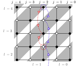
Figure S1: The coordinate system used for the square lattice, labelling vertical chains with $j$ and each second diagonal with $l$. The Jordan-Wigner string for $a_{1}$ ($b_{3}$), enclosed by the blue (red) circle, is represented by the blue (red) dashed line.

Now we can apply the standard bosonization technique Giamarchi (2003). The low-energy effective Hamiltonian is given by the free boson theory,

$$H_{\textrm{eff}}\sim\int dx\sum_{s=a,b}\frac{v^{s}}{2\pi}\left[(\partial_{x}\varphi^{s})^{2}+(\partial_{x}\theta^{s})^{2}\right],$$ (S8)

where $v^{s}=2t_{\perp}\sin(\pi\langle n^{s}\rangle)$, $x=\ell d_{0}$ with $d_{0}$ being the lattice spacing, and the bosonic fields satisfy the commutation relations,

$$[\theta^{s}(x),\varphi^{s^{\prime}}(x^{\prime})]=i\pi\delta_{ss^{\prime}}\Theta(x-x^{\prime}),$$ (S9)

with $\Theta(x)$ being the Heaviside step function. The lattice boson operators are expressed in terms of the bosonic fields as

$$\tilde{a}_{\ell} \sim e^{-i\varphi^{a}(x)}\sum_{m\geq 0}C^{a}_{2m}\cos\left(2m\theta^{a}(x)+2\pi m\langle n^{a}\rangle\ell\right),$$ (S10)

$$\tilde{b}_{\ell} \sim e^{-i\varphi^{b}(x)}\sum_{m\geq 0}C^{b}_{2m}\cos\left(2m\theta^{b}(x)+2\pi m\langle n^{b}\rangle\ell\right),$$ (S11)

$$\tilde{n}^{s}_{\ell} \sim\langle n^{s}\rangle+\frac{d_{0}}{\pi}\partial_{x}\theta^{s}(x)+\cdots.$$ (S12)

The string operators may also be expressed as

$$\tilde{K}^{a}_{\ell} \sim\sum_{m\geq 0}D^{a}_{2m+1}\cos\left[(2m+1)\theta^{a}(x)+\pi(2m+1)\langle n^{a}\rangle\ell\right],$$ (S13)

$$\tilde{K}^{b}_{\ell} \sim\sum_{m\geq 0}D^{b}_{2m+1}\cos\left[(2m+1)(\theta^{b}(x)-\pi N^{b})+\pi(2m+1)\langle n^{b}\rangle\ell\right].$$ (S14)

Here $C^{s}_{2m}$ and $D^{s}_{2m+1}$ are numerical constants and $N^{s}$ are zero-mod operators formally defined by

$$N^{s}=\int^{\infty}_{-\infty}dx\frac{1}{\pi}\partial_{x}\theta^{s}(x).$$ (S15)

Let us consider the single particle correlation functions $\langle a^{\dagger}_{\ell}a_{\ell^{\prime}}\rangle$ and $\langle b^{\dagger}_{\ell}b_{\ell^{\prime}}\rangle$. In our free boson theory, the vertex operators $e^{im\varphi^{s}(x)}$ and $e^{im\theta^{s}(x)}$ both have scaling dimension $m^{2}/4$. Using Eqs. (S5) and (S10)-(S14) and keeping only most slowly decaying parts, we find

$$\langle a^{\dagger}_{\ell}a_{\ell^{\prime}}\rangle \sim\frac{C^{a}_{0}D^{b}_{1}}{4}\left(\frac{e^{i(\frac{\pi}{2}+\pi\langle n^{b}\rangle)(\ell-\ell^{\prime})}}{|\ell-\ell^{\prime}|}+\frac{e^{i(\frac{\pi}{2}-\pi\langle n^{b}\rangle)(\ell-\ell^{\prime})}}{|\ell-\ell^{\prime}|}\right)+\cdots,$$ (S16)

$$\langle b^{\dagger}_{\ell}b_{\ell^{\prime}}\rangle \sim\frac{C^{b}_{0}D^{a}_{1}}{4}\left(\frac{e^{i(-\frac{\pi}{2}+\pi\langle n^{a}\rangle)(\ell-\ell^{\prime})}}{|\ell-\ell^{\prime}|}+\frac{e^{i(-\frac{\pi}{2}-\pi\langle n^{a}\rangle)(\ell-\ell^{\prime})}}{|\ell-\ell^{\prime}|}\right)+\cdots.$$ (S17)

The momentum distribution functions are obtained by their Fourier transforms: $\langle n^{a}(k)\rangle=\langle a^{\dagger}(k)a(k)\rangle$. They diverge logarithmically as $k$ approaches $\frac{\pi}{2}\pm\pi\langle n^{b}\rangle$ for the $A$ sublattice and $-\frac{\pi}{2}\pm\pi\langle n^{a}\rangle$ for the $B$ sublattice,

$$\langle n^{a}(k)\rangle\sim\log\frac{1}{|k-\frac{\pi}{2}\mp\pi\langle n^{b}\rangle|},\ \ \ \langle n^{b}(k)\rangle\sim\log\frac{1}{|k+\frac{\pi}{2}\mp\pi\langle n^{a}\rangle|}.$$ (S18)

The positions of the singularities depend on the boson density of different species. This behavior is contrasted from that for the standard hard-core boson chain, $H=-t\sum_{\ell}(a^{\dagger}_{\ell}a_{\ell+1}+\textrm{H.c.})$, for which the momentum distribution function exhibits a power-law divergence $\langle n^{a}(k)\rangle\sim|k|^{-1/2}$ as $k\to 0$ Giamarchi (2003).

II.2 Coupled wire Hamiltonian

We are now in a position to study the low-energy physics of the correlated hopping chains weakly coupled by $J_{\parallel}$ in the spirit of coupled-wire construction Kane et al. (2002); Teo and Kane (2014); Lu and Vishwanath (2012). We start from the decoupled chain Hamiltonian,

$$H^{0}_{\textrm{eff}}=t_{\perp}\sum_{j,\ell}\left[ia^{\dagger}_{j,\ell}a_{j,\ell+1}(2n^{b}_{j,\ell}-1)-ib^{\dagger}_{j,\ell}b_{j,\ell+1}(2n^{a}_{j,\ell+1}-1)+\textrm{H.c.}\right],$$ (S19)

where the site index $(j,\ell)$ is assigned in the way depicted in Fig. S1. With this assignment and choosing a Landau gauge to implement the flux $\phi$ for each square plaquette, the effective Floquet Hamiltonian involving $J_{\parallel}$ couplings is given by

$$H^{1}_{\textrm{eff}} =t_{\parallel}\sum_{j,\ell}\left[-ie^{-i\phi(2\ell)}a^{\dagger}_{j,\ell}a_{j+1,\ell}(2n^{b}_{j+1,\ell}-1)+ie^{-i\phi(2\ell+1)}a^{\dagger}_{j,\ell}a_{j+1,\ell+1}(2n^{b}_{j,\ell}-1)\right.$$

$$\left.+ie^{-i\phi(2\ell)}b^{\dagger}_{j,\ell}b_{j+1,\ell}(2n^{a}_{j,\ell}-1)-ie^{-i\phi(2\ell+1)}b^{\dagger}_{j,\ell}b_{j+1,\ell+1}(2n^{a}_{j+1,\ell+1}-1)+\textrm{H.c.}\right],$$ (S20)

where $t_{\parallel}=2J_{\perp}J_{\parallel}/\Omega$. Applying the Jordan-Wigner transformation (S5) for each chain, we find

$$H^{0}_{\textrm{eff}} =-t_{\perp}\sum_{j,\ell}\left(\tilde{a}_{j,\ell}^{\dagger}\tilde{a}_{j,\ell+1}+\tilde{b}^{\dagger}_{j,\ell}\tilde{b}_{j,\ell+1}+\textrm{H.c.}\right),$$ (S21)

$$H^{1}_{\textrm{eff}} =-t_{\parallel}\sum_{j,\ell}\left(-ie^{-i\phi(2\ell)}\tilde{a}^{\dagger}_{j,\ell}\tilde{a}_{j+1,\ell}\tilde{K}^{b}_{j,\ell}\tilde{K}^{b}_{j+1,\ell+1}+e^{-i\phi(2\ell+1)}\tilde{a}^{\dagger}_{j,\ell}\tilde{a}_{j+1,\ell+1}\tilde{K}^{b}_{j,\ell+1}\tilde{K}^{b}_{j+1,\ell+1}\right.$$

$$\left.+ie^{-i\phi(2\ell)}\tilde{b}^{\dagger}_{j,\ell}\tilde{b}_{j+1,\ell}\tilde{K}^{a}_{j,\ell-1}\tilde{K}^{a}_{j+1,\ell}+e^{-i\phi(2\ell+1)}\tilde{b}^{\dagger}_{j,\ell}\tilde{b}_{j+1,\ell+1}\tilde{K}^{a}_{j,\ell}\tilde{K}^{a}_{j+1,\ell}+\textrm{H.c.}\right).$$ (S22)

For $|J_{\parallel}|\ll|J_{\perp}|$, we can treat $H^{1}_{\textrm{eff}}$ as perturbations and apply the above bosonization procedure to obtain the low-energy effective Hamiltonian as similarly done in Ref. Fuji et al. (2016). Keeping only terms relevant for quantum Hall states, we find

$$H^{0}_{\textrm{eff}} \sim\int dx\sum_{j}\sum_{s=a,b}\frac{v^{s}}{2\pi}\left[(\partial_{x}\varphi^{s}_{j})^{2}+(\partial_{x}\theta^{s}_{j})^{2}\right],$$

$$H^{1}_{\textrm{eff}} \sim-\sum_{p\in\mathbb{Z}}\sum_{q\in\mathbb{Z}}\sum_{j}\int dx\left[g^{a}_{(p,q)}e^{i\pi(2q+1)\langle n^{b}\rangle}(-i+e^{-i\Gamma^{a}_{(p,q)}})e^{-2i\Gamma^{a}_{(p,q)}x/d_{0}}e^{i\chi^{a}_{(p,q),j}(x)-i\tilde{\chi}^{a}_{(p,q),j+1}(x)}\right.$$

$$\left.+g^{b}_{(p,q)}e^{-i\pi(2q+1)\langle n^{a}\rangle}(i+e^{-i\Gamma^{b}_{(p,q)}})e^{-2i\Gamma^{b}_{(p,q)}x/d_{0}}e^{i\chi^{b}_{(p,q),j}(x)-i\tilde{\chi}^{b}_{(p,q),j+1}(x)}+\textrm{H.c.}\right]+\cdots,$$ (S23)

where the bosonic fields satisfy the commutation relations $[\theta^{s}_{j}(x),\varphi^{s^{\prime}}_{j^{\prime}}(x^{\prime})]=i\pi\delta_{ss^{\prime}}\delta_{jj^{\prime}}\Theta(x-x^{\prime})$ and we have defined $g^{s}_{(p,q)}$, $\Gamma^{s}_{(p,q)}$, $\chi^{s}_{(p,q),j}(x)$, and $\tilde{\chi}^{s}_{(p,q),j}(x)$ by

$$g^{a}_{(p,q)} =\frac{t_{\parallel}(C^{a}_{|2p|}D^{b}_{|2q+1|})^{2}}{4},\ \ \ g^{b}_{(p,q)}=\frac{t_{\parallel}(C^{b}_{|2p|}D^{a}_{|2q+1|})^{2}}{4},$$ (S24)

$$\Gamma^{a}_{(p,q)} =\phi-\pi(2p)\langle n^{a}\rangle-\pi(2q+1)\langle n^{b}\rangle,\ \ \ \Gamma^{b}_{(p,q)}=\phi-\pi(2p)\langle n^{b}\rangle-\pi(2q+1)\langle n^{a}\rangle,$$ (S25)

$$\begin{split}\chi^{a}_{(p,q),j}(x)&=\varphi^{a}_{j}(x)+2p\theta^{a}_{j}(x)+(2q+1)(\theta^{b}_{j}(x)-\pi N^{b}_{j}),\\ \chi^{b}_{(p,q),j}(x)&=\varphi^{b}_{j}(x)+2p\theta^{b}_{j}(x)+(2q+1)\theta^{a}_{j}(x),\\ \tilde{\chi}^{a}_{(p,q),j}(x)&=\varphi^{a}_{j}(x)-2p\theta^{a}_{j}(x)-(2q+1)(\theta^{b}_{j}(x)-\pi N^{b}_{j}),\\ \tilde{\chi}^{b}_{(p,q),j}(x)&=\varphi^{b}_{j}(x)-2p\theta^{b}_{j}(x)-(2q+1)\theta^{a}_{j}(x).\end{split}$$ (S26)

If the couplings $g^{a}_{(p,q)}$ and $g^{b}_{(p,q)}$ both flow to the strong-coupling fixed point, it is possible to find a quantum Hall state described by the $2\times 2$ $K$ matrix Wen (1995),

$$K=\begin{pmatrix}2p&2q+1\\ 2q+1&2p\end{pmatrix}.$$ (S27)

This can be understood by the fact that the bosonic fields $\tilde{\chi}^{s}_{(p,q),j}(x)$ and $\chi^{s}_{(p,q),j}(x)$ are left unpaired and remain gapless at the outermost wires $j=1$ and $N_{w}$, respectively, while they are gapped elsewhere in the bulk $1<j<N_{w}$. These bosonic fields satisfy the commutation relations,

$$[\partial_{x}\chi^{s}_{(p,q),j}(x),\chi^{s^{\prime}}_{(p,q),j^{\prime}}(x^{\prime})]=-[\partial_{x}\tilde{\chi}^{s}_{(p,q),j}(x),\tilde{\chi}^{s^{\prime}}_{(p,q),j^{\prime}}(x^{\prime})]=2i\pi K_{ss^{\prime}}\delta_{jj^{\prime}}\delta(x-x^{\prime}),$$ (S28)

as expected from the Chern-Simons theory Wen (1995). To obtain the quantum Hall states, several remarks are in order. For given $p$ and $q$, the flux $\phi$ and the boson densities $\langle n^{s}\rangle$ must satisfy the commensurability condition $\Gamma^{s}_{(p,q)}\equiv 0$ for the corresponding interactions to slowly vary in $x$. This requires

$$\begin{split}\phi&=\pi(2p)\langle n^{a}\rangle+\pi(2q+1)\langle n^{b}\rangle\mod\pi,\\ \phi&=\pi(2p)\langle n^{b}\rangle+\pi(2q+1)\langle n^{a}\rangle\mod\pi.\end{split}$$ (S29)

We also note that in the perturbatively accessible regime $|J_{\parallel}|\ll|J_{\perp}|$, only the coupling constants with $(p,q)=(0,0)$ or $(0,-1)$ become relevant in the renormalization group sense. This corresponds to the BIQH state, the focus of the main text. Indeed, the choice of parameters $\langle n^{a}\rangle=\langle n^{b}\rangle\equiv\langle n\rangle=1/2$ and $\phi=\pi/2$ used for the numerical study meets the above commensurability conditions. However, at the small system sizes accessible to numerics, we have of course not yet reached the strong-coupling fixed point. This explains why at perturbatively small $J_{\parallel}/J_{\perp}$ we observe a superfluid phase, but at large enough $J_{\parallel}/J_{\perp}$ there is a phase transition into a BIQH state.

II.3 Mutual flux attachment for BIQH state

The mutual flux attachment proposed in Ref. Senthil and Levin (2013) is nicely furnished in our coupled-wire system for the BIQH state without any uncontrollable approximation. The following argument is strongly inspired from a recent study of duality web in Ref. Mross et al. (2017). We now define the “mutual composite boson” fields by a nonlocal transformation Fuji and Furusaki (2019),

$$\Phi^{a}_{j}(x) =\varphi^{a}_{j}(x)+\sum_{j^{\prime}\neq j}\textrm{sgn}(j^{\prime}-j)(\theta^{b}_{j^{\prime}}(x)-\pi N^{b}_{j^{\prime}}),$$ (S30)

$$\Phi^{b}_{j}(x) =\varphi^{b}_{j}(x)+\sum_{j^{\prime}\neq j}\textrm{sgn}(j^{\prime}-j)\theta^{a}_{j^{\prime}}(x),$$ (S31)

$$\Theta^{s}_{j}(x) =\theta^{s}_{j}(x).$$ (S32)

They satisfy the commutation relations,

$$\begin{split}[\Theta^{a}_{j}(x),\Phi^{a}_{j^{\prime}}(x^{\prime})]&=i\pi\delta_{jj^{\prime}}\Theta(x-x^{\prime}),\\ [\Theta^{b}_{j}(x),\Phi^{b}_{j^{\prime}}(x^{\prime})]&=i\pi\delta_{jj^{\prime}}[\Theta(x-x^{\prime})-1]\end{split}$$ (S33)

while the other commutators vanish. We then consider the Euclidean action corresponding to the decoupled chain Hamiltonian (II.2),

$$S_{0}=\int d\tau dx\sum_{j}\sum_{s=a,b}\left[\frac{i}{\pi}\partial_{x}\theta^{s}_{j}\partial_{\tau}\varphi^{s}_{j}+\frac{v^{s}}{2\pi}\left\{(\partial_{x}\varphi^{s}_{j})^{2}+(\partial_{x}\theta^{s}_{j})^{2}\right\}\right].$$ (S34)

In terms of the mutual composite boson fields, the action is written as

$$S_{0}=\int d\tau dx\sum_{j}\sum_{s=a,b}\biggl{[}\frac{i}{\pi}\partial_{x}\Theta^{s}_{j}\partial_{\tau}\Phi^{s}_{j}+\frac{v^{s}}{2\pi}\Bigl{\{}\Bigl{(}\partial_{x}\Phi^{s}_{j}-\sum_{j^{\prime}\neq j}\textrm{sgn}(j^{\prime}-j)\partial_{x}\Theta^{s^{\prime}}_{j}\Bigr{)}^{2}+(\partial_{x}\Theta^{s}_{j})^{2}\Bigr{\}}\biggr{]},$$ (S35)

where $s^{\prime}=b(a)$ for $s=a(b)$. To formally resolve the nonlocality of this action, we define auxiliary fields $a^{1}_{1,j}$ and $a^{2}_{1,j}$ by

$$a^{1}_{1,j}=\sum_{j^{\prime}\neq j}\textrm{sgn}(j^{\prime}-j)\partial_{x}\Theta^{b}_{j^{\prime}},\ \ \ a^{2}_{1,j}=\sum_{j^{\prime}\neq j}\textrm{sgn}(j^{\prime}-j)\partial_{x}\Theta^{a}_{j^{\prime}},$$ (S36)

and implement these constraints by Lagrange multipliers $a^{1}_{0,j+\frac{1}{2}}$ and $a^{2}_{0,j+\frac{1}{2}}$ as

$$S_{\textrm{LM}} =\int d\tau dx\sum_{j}\frac{i}{2\pi}\biggl{[}(a^{1}_{0,j+\frac{1}{2}}-a^{1}_{0,j-\frac{1}{2}})\Bigl{\{}a^{2}_{1,j}-\sum_{j^{\prime}\neq j}\textrm{sgn}(j^{\prime}-j)\partial_{x}\Theta^{a}_{j^{\prime}}\Bigr{\}}$$

$$+(a^{2}_{0,j+\frac{1}{2}}-a^{2}_{0,j-\frac{1}{2}})\Bigl{\{}a^{1}_{1,j}-\sum_{j^{\prime}\neq j}\textrm{sgn}(j^{\prime}-j)\partial_{x}\Theta^{b}_{j^{\prime}}\Bigr{\}}\biggr{]}.$$ (S37)

After some algebra, the action $S^{\prime}_{0}=S_{0}+S_{\textrm{LM}}$ is expressed as

$$S^{\prime}_{0} =\int d\tau dx\sum_{j}\Biggl{[}\frac{i}{\pi}\partial_{x}\Theta^{a}_{j}\biggl{(}\partial_{\tau}\Phi^{a}_{j}-\frac{a^{1}_{0,j+\frac{1}{2}}+a^{1}_{0,j-\frac{1}{2}}}{2}\biggr{)}+\frac{i}{\pi}\partial_{x}\Theta^{b}_{j}\biggl{(}\partial_{\tau}\Phi^{b}_{j}-\frac{a^{2}_{0,j+\frac{1}{2}}+a^{2}_{0,j-\frac{1}{2}}}{2}\biggr{)}$$

$$+\frac{v^{a}}{2\pi}\Bigl{\{}(\partial_{x}\Phi^{a}_{j}-a^{1}_{1,j})^{2}+(\partial_{x}\Theta^{a}_{j})^{2}\Bigr{\}}+\frac{v^{b}}{2\pi}\Bigl{\{}(\partial_{x}\Phi^{b}_{j}-a^{2}_{1,j})^{2}+(\partial_{x}\Theta^{b}_{j})^{2}\Bigr{\}}$$

$$+\frac{i}{4\pi}\Bigl{\{}a^{1}_{1,j}(a^{2}_{0,j+\frac{1}{2}}-a^{2}_{0,j-\frac{1}{2}})-a^{2}_{0,j+\frac{1}{2}}(a^{1}_{1,j+1}-a^{1}_{1,j})\Bigr{\}}+\frac{i}{4\pi}\Bigl{\{}a^{2}_{1,j}(a^{1}_{0,j+\frac{1}{2}}-a^{1}_{0,j-\frac{1}{2}})-a^{1}_{0,j+\frac{1}{2}}(a^{2}_{1,j+1}-a^{2}_{1,j})\Bigr{\}}\Biggr{]}.$$ (S38)

This action can be seen as a discrete analog of two-component bosonic fields minimally coupled with the mutual Chern-Simons term $\frac{i}{4\pi}\epsilon^{\mu\nu\lambda}(a^{1}_{\mu}\partial_{\nu}a^{2}_{\lambda}+a^{2}_{\mu}\partial_{\nu}a^{1}_{\lambda})$ under the gauge choice $a^{1}_{2}=a^{2}_{2}=0$. We also consider interchain interactions corresponding to the BIQH state with $(p,q)=(0,0)$,

$$H_{1} =-\int dx\sum_{j}\left[g^{a}\cos\left(\varphi^{a}_{j}+\theta^{b}_{j}-\pi N^{b}_{j}-\varphi^{a}_{j+1}+\theta^{b}_{j+1}-\pi N^{b}_{j+1}\right)+g^{b}\cos\left(\varphi^{b}_{j}+\theta^{a}_{j}-\varphi^{b}_{j+1}+\theta^{a}_{j+1}\right)\right]$$

$$=-\int dx\sum_{j}\left[g^{a}\cos\left(\Phi^{a}_{j}-\Phi^{a}_{j+1}\right)+g^{b}\cos\left(\Phi^{b}_{j}-\Phi^{b}_{j+1}\right)\right].$$ (S39)

The interactions maintain a local form in terms of the mutual composite boson fields. According to Eq. (S33), the operators $e^{i\Phi^{s}_{j}(x)}$ can be viewed as bosonic particle operators and thus the interactions can induce a condensation. This precisely reproduces the argument of Ref. Senthil and Levin (2013) which states that the BIQH state is obtained by the condensation of composite bosons with the mutual $2\pi$ flux attachment.

III Numerical Methods

The numerical simulations are carried out using DMRG algorithm of TenPy library Hauschild and Pollmann (2018). The 2D lattice is placed on an infinitely long cylinder of width $L$ sites, with periodic boundary conditions in both direction. For the honeycomb lattice, ”Cstyle” ordering of the MPS is used.

Imposing the symmetries of the Hamiltonian by conserving charges in tensor network methods leads to large speedups and reduction in memory usage. However, enforcing too many restrictions could, in turn, result in the algorithm getting stuck in local minima. In our simulations, we find that explicitly imposing the $U(1)\times U(1)$ symmetry, i.e. particle number conservation on each sublattice, would sometimes lead to failure of DMRG in finding the correct ground state. Thus, we conserve the total particle number only. However, we carefully confirmed that in all cases the final ground state obtained does not break the full $U(1)\times U(1)$ symmetry explicitly.

To implement the background flux on the honeycomb lattice, we utilize the same gauge choice as Ref. He et al. (2015a) for the next-nearest-neighbor couplings. On the square lattice, we use a Landau gauge for the choice of nearest-neighbor $B_{ik}$, and set $B_{ij}=B_{ik}+B_{kj}$ (as defined in the derivation of Eq. S0.Ex1) for the the next-nearest-neighbor correlated hoppings $(2n^{b}_{k}-1)a^{\dagger}_{i}a_{j}$.

IV Effects of system size

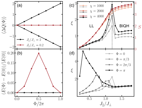
Figure S2: Numerical study of the correlated hopping model on the square lattice with half filling and background flux $\phi=\pi/2$, simulated on a cylinder of width $L=8$ sites. (a) Charge pumping under flux threading. (b) Energy response under flux threading. (c) Correlation length and entanglement entropy, showing a phase transition from a Luttinger liquid to BIQH with increasing $J_{\parallel}/J_{\perp}$. (d) Shifting of the critical point to smaller values of $J_{\parallel}/J_{\perp}$ as the threaded flux increases from $\Phi=0$ to $\pi$.

The iDMRG results shown in the main text for the square lattice with half filling and background flux $\phi=\pi/2$ are all obtained for system size $L=10$. While we have numerical evidence for the existence of the BIQH phase on systems of size $L=6,8,10$ [Fig. S2(a)], the phase diagram exhibits a marked difference for system sizes where $L/2$ is even or odd (compare Fig.S3(a) to Fig.1(c)). This might be expected from the coupled chain picture: when $L/2$ is even, the system has a finite size gap which is not present in the odd case. In this section, we analyze the phase diagram for the even case by focusing on system size $L=8$.

One major difference between the even and the odd case is the nature of the phase to the left of BIQH. The coupled wire analysis in the previous section predicts that an infinitesimal coupling $J_{\parallel}$ should drive the system into a BIQH state. However, the correlation length and entanglement entropy data in Fig.S2(c) suggests that the transition into the BIQH phase happens around $J_{\parallel}/J_{\perp}=1.2$. Then a natural question arises: Is there an intermediate phase between the decoupled LL at $J_{\parallel}=0$ and the BIQH phase? or should one think of this ”intermediate phase” as one that is smoothly connected to the decoupled LL whose existence is due to the energy gap present at our finite size simulations?

Our numerical data supports the latter description for systems of even size, unlike the odd case. First, the correlation length connects smoothly to zero as $J_{\parallel}/J_{\perp}$ decreases from $1$ to $0$ [Fig. S2(c)], compared to the odd case where it diverges[Fig. 3(a)]. Furthermore, the large energy dispersion under flux insertion at $J_{\parallel}/J_{\perp}=0.2$ [Fig. S2(b)] suggests that the state is gapless, which is consistent with the case of decoupled LLs. lastly, the correlation length data in Fig. S2(d) shows the critical point moving towards the decoupling limit as the inserted flux $\Phi$ is increased. This is also consistent with the decoupled LL scenario because the gap decreases with inserted flux and the results should more closely match what we expect to see in the thermodynamic limit.

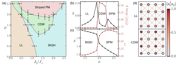
Figure S3: (a) Phase diagram of the correlated hopping model on the square lattice with half filling and background flux $\phi=\pi/2$, as a function of $J_{\parallel}/J_{\perp}$ and striped potential $\mu$, simulated on a cylinder of width $L=8$ sites. (b) Entanglement entropy and the variance of density in the perpendicular direction along a cut at fixed $J_{\parallel}/J_{\perp}=0.5$. (c) Entanglement entorpy and correlation length along a cut at fixed $J_{\parallel}/J_{\perp}=2$. (d) Density and nearest-neighbor correlations for the LL at $J_{\parallel}/J_{\perp}=0.5,\mu=0$ and the CDW at $J_{\parallel}/J_{\perp}=0.5,\mu=2.1$.

As shown in Fig.S3, another major difference between the even and the odd case is the markedly distinct behavior of the system upon increasing $\mu$ for $1\lesssim J_{\parallel}/J_{\perp}\lesssim 2$. Rather than transitioning directly to the striped paramagnet phase from the BIQH phase, there appears to be an intermediate spontaneous symmetry-breaking phase. This phase exhibits the same striped pattern as the paramagnet, but also spontaneously breaks symmetry in the perpendicular direction. The associated charge density wave (CDW) pattern is characterized by an order parameter measuring the variance of the density in the perpendicular direction [Fig S3(b)]. Much like the shaded region in Fig. 1(c) in the main text, we caution that the region between the Luttinger Liquid phase and striped paramagnetic phase is difficult to converge in bond dimension due to its proximity to multiple phase transitions. It is possible, therefore, that the CDW does not represent the true ground state in the thermodynamic limit for all the green shaded region in Fig. S3(a). The presence of a strongly diverging correlation length as well as the smooth decrease in the order parameter suggests that the CDW-SPM transition is continuous. Meanwhile, the correlation length at the BIQH-CDW transition is only weakly enhanced as a function of the iDMRG bond dimension, and there is a sharp increase in the order parameter, consistent with the possibility of a first order phase transition; this is further supported by wave function overlap calculations.

V Experimental realization of the Floquet scheme

The set up in Fig.4 consists of four independent pairs of laser beams labeled as $\gamma=\{1,2,3,4\}$ (only two are shown for simplicity). Each pair consists of two vertically-polarized laser beams that are retro reflected and aligned along the primary axes of the lattice ($x$ and $y$ axis),

$$\textbf{E}_{\parallel}^{\gamma}(\textbf{r},t)= 2E_{x}\text{e}^{i\omega_{\parallel}^{\gamma}t}\cos(kx+\varphi_{x}^{\gamma})$$ (S40)

$$\textbf{E}_{\perp}^{\gamma}(\textbf{r},t)= 2E_{y}\text{e}^{i[(\omega_{\perp}^{\gamma}+\Omega)t+\theta_{0}^{\gamma}]}\cos(ky+\varphi_{y}^{\gamma})$$ (S41)

$$+ 2E_{y}\text{e}^{i[(\omega_{\perp}^{\gamma}-\Omega)t-\theta_{0}^{\gamma}]}\cos(ky+\varphi_{y}^{\gamma})$$

$$= 4E_{y}\text{e}^{i\omega_{\perp}^{\gamma}t}\cos(\Omega t+\theta_{0}^{\gamma})\cos(ky+\varphi_{y}^{\gamma}),$$

with the wave vectors chosen to be $|\mathbf{k}_{\parallel}|\simeq|\mathbf{k}_{\perp}|=k=\frac{\pi}{2a}$, where $a$ is the lattice constant. The laser beams along $y$ have two frequency components $\omega^{\gamma}_{\perp}\pm\Omega$ and the ones along $x$ a single component at $\omega^{\gamma}_{\perp}$, with $\omega^{\gamma}_{\perp}-\omega^{\gamma}_{\parallel}=\omega=\Delta_{y}/\hbar$ resonant with the potential energy difference between neighboring sites. The total time-dependent potential that results from the interference of these beams consists of several terms $V_{\text{tot}}=V_{\text{cst}}+V_{2\Omega}+V_{\text{cross}}$. A constant part

$$V^{\gamma}_{\text{cst}}=4E_{x}^{2}\cos^{2}(kx+\varphi_{x}^{\gamma})+8E_{y}^{2}\cos^{2}(ky+\varphi_{y}^{\gamma}),$$ (S42)

and the second term

$$V^{\gamma}_{2\Omega}=8E_{y}^{2}\cos(2\Omega t+2\theta_{0}^{\gamma})\cos^{2}(ky+\varphi_{y}^{\gamma}),$$ (S43)

which generates a modulation at $2\Omega$. We will re-examine both terms at the end of this section. What we are interested in is the cross term

$$V^{\gamma}_{\text{cross}}=16E_{x}E_{y}\cos(\omega t)\cos(\Omega t+\theta_{0}^{\gamma})\cos(kx+\varphi_{x}^{\gamma})\cos(ky+\varphi_{y}^{\gamma}),$$ (S44)

In the high frequency limit $\omega\gg\Omega$, the term $\cos(\Omega t+\theta_{0}^{\gamma})$ can be treated as constant and the dynamics are described by

$$H(t)= -\sum_{m,n}\left(J_{x}\hat{a}^{\dagger}_{m+1,n}\hat{a}_{m,n}+J_{y}\hat{a}^{\dagger}_{m,n+1}\hat{a}_{m,n}+\text{h.c.}\right)$$ (S45)

$$+\sum_{m,n}\left(n\Delta_{y}+\sum_{\gamma}V_{0}^{\gamma}\cos(\omega t)\cos(m\frac{\pi}{2}+\varphi_{x}^{\gamma})\cos(n\frac{\pi}{2}+\varphi_{y}^{\gamma})\right)\hat{n}_{m,n},$$

where $m$ ($n$) is the lattice site index along $x$ ($y$), $V_{0}^{\gamma}=16E_{x}E_{y}\cos(\Omega t+\theta_{0}^{\gamma})$. This Hamiltonian is periodic and can be approximated using a Floquet-Magnus expansion. The static term of the Hamiltonian contains diverging components proportional to $\hbar\omega=\Delta_{y}$. Therefore a transformation into the rotating frame is performed using the unitary operator

$$R_{M}(t) =\exp\left[i\sum_{m,n}\left(\frac{n\Delta_{y}t}{\hbar}+\sum_{\gamma}\frac{V_{0}^{\gamma}}{\hbar\omega}\sin(\omega t)\cos(m\frac{\pi}{2}+\varphi_{x}^{\gamma})\cos(n\frac{\pi}{2}+\varphi_{y}^{\gamma})\right)\hat{n}_{m,n}\right]$$ (S46)

$$=\exp\left[i\sum_{m,n}\chi_{m,n}(t)\hat{n}_{m,n}\right].$$

The transformed Hamiltonian can be written in the following form,

$$H_{M}(t)= -\sum_{m,n}\left(J_{x}e^{i\eta^{x}_{m,n}(t)}\hat{a}^{\dagger}_{m+1,n}\hat{a}_{m,n}+J_{y}e^{i\eta^{y}_{m,n}(t)}\hat{a}^{\dagger}_{m,n+1}\hat{a}_{m,n}+\text{h.c.}\right),$$ (S47)

with $\eta^{x}_{m,n}(t)=\chi_{m+1,n}(t)-\chi_{m,n}(t)$ and $\eta^{y}_{m,n}(t)=\chi_{m,n+1}(t)-\chi_{m,n}(t)$ given by

$$\eta^{x}_{m,n}(t) =-\eta^{x}_{0}\sin(\omega t)$$ (S48)

$$\eta^{y}_{m,n}(t) =-\eta^{y}_{0}\sin(\omega t)+\frac{\Delta_{y}t}{\hbar},$$ (S49)

where we have defined

$$\eta^{x}_{0} =\sum_{\gamma}\frac{\sqrt{2}V_{0}^{\gamma}}{\hbar\omega}\cos(n\frac{\pi}{2}+\varphi_{y}^{\gamma})\sin(m\frac{\pi}{2}+\frac{\pi}{4}+\varphi_{x}^{\gamma})$$ (S50)

$$\eta^{y}_{0} =\sum_{\gamma}\frac{\sqrt{2}V_{0}^{\gamma}}{\hbar\omega}\cos(m\frac{\pi}{2}+\varphi_{x}^{\gamma})\sin(n\frac{\pi}{2}+\frac{\pi}{4}+\varphi_{y}^{\gamma}).$$ (S51)

The lowest order of the time-independent Floquet Hamiltonian using the Magnus expansion is thus given by

$$H_{F} =\frac{1}{T}\int_{0}^{T}H_{M}(t)dt$$

$$=-\frac{1}{2\pi}\sum_{m,n}\left(J_{x}\hat{a}^{\dagger}_{m+1,n}\hat{a}_{m,n}\int_{0}^{2\pi}e^{-i\eta^{x}_{0}\sin{\tau}}d\tau+J_{y}\hat{a}^{\dagger}_{m,n+1}\hat{a}_{m,n}\int_{0}^{2\pi}e^{i(\tau-\eta^{y}_{0}\sin{\tau})}d\tau+\text{h.c.}\right)$$

$$=-\sum_{m,n}\left(J_{x}\mathcal{J}_{0}(\eta^{x}_{0})\hat{a}^{\dagger}_{m+1,n}\hat{a}_{m,n}+J_{y}\mathcal{J}_{1}(\eta^{y}_{0})\hat{a}^{\dagger}_{m,n+1}\hat{a}_{m,n}+\text{h.c.}\right)$$ (S52)

where $\mathcal{J}_{\nu}(x)=\frac{1}{2\pi}\int_{0}^{2\pi}e^{i(\nu\tau-x\sin{\tau})}d\tau$ is the $\nu$th order Bessel function of the first kind. Using the expansion $\mathcal{J}_{\nu}(x)=\sum_{n}\frac{(-1)^{n}}{n!(n+\nu)!}(\frac{x}{2})^{2n+\nu}$, the Bessel functions can be approximated to the first order by $\mathcal{J}_{0}(x)\simeq 1$ and $\mathcal{J}_{1}(x)\simeq x/2$ for $x\ll 1$. Thus, in the limit $V_{0}\ll\hbar\omega$, the effective Hamiltonian is given by

$$H_{F}\simeq-\sum_{m,n}(J_{x}\hat{a}^{\dagger}_{m+1,n}\hat{a}_{m,n}+J_{y}^{\text{eff}}\hat{a}^{\dagger}_{m,n+1}\hat{a}_{m,n}+\text{h.c.}),$$ (S53)

with

$$J_{y}^{\text{eff}}=J_{y}\frac{\eta^{y}_{0}}{2}=J_{y}\frac{8\sqrt{2}E_{x}E_{y}}{\Delta_{y}}\sum_{\gamma}\cos(\Omega t+\theta_{0}^{\gamma})\cos(m\frac{\pi}{2}+\varphi_{x}^{\gamma})\sin(n\frac{\pi}{2}+\frac{\pi}{4}+\varphi_{y}^{\gamma}).$$ (S54)

As desired, the effective coupling strength depends on $\cos(\Omega t+\theta_{0}^{\gamma})$ and the spatial dependence $\cos(m\frac{\pi}{2}+\varphi_{x}^{\gamma})\sin(n\frac{\pi}{2}+\frac{\pi}{4}+\varphi_{y}^{\gamma})$ allows us to separately address the bonds with different values of $\theta_{0}^{\gamma}$. With the choice of $(\varphi_{x}^{\gamma},\varphi_{y}^{\gamma})=\{(0,\pi/4),(\pi/2,-\pi/4),(\pi,3\pi/4),(\pi/2,\pi/4)\}$, we can address the red(dashed), blue(dashed), blue(solid), and red(solid) bonds respectively [Fig. S4(c)]. We then set $\theta_{0}^{\gamma}=\pi/2$ for dashed lines and $\theta_{0}^{\gamma}=0$ for solid lines. Note that, under these parameters, the spatial dependence of $V^{\gamma}_{\text{cst}}$ and $V^{\gamma}_{2\Omega}$ for the combined setup gets cancelled and we obtain

$$\sum_{\gamma}{V^{\gamma}_{\text{cst}}} =8E_{x}^{2}+16E_{y}^{2}$$ (S55)

$$\sum_{\gamma}{V^{\gamma}_{2\Omega}} =0.$$ (S56)

The oscillation of the cos()sin() term in Eq. S54 between $\pm 1$ results in a staggered background flux $\phi=0,\pi$. In order to acquire a homogeneous flux as well as the amplitude modulation on the horizontal bonds, we repeat the same technique of laser-assisted tunneling in the perpendicular direction [Fig. S4(a,b)], by adding a staggered potential $\Delta_{m}=(-1)^{m}\Delta_{x}/2$ along the $x$ axis. A pair of running lasers with $\omega_{\perp}-\omega_{\parallel}=\omega=\Delta_{x}/\hbar$ is then used to restore the tunneling.

$$\textbf{E}_{\parallel}(\textbf{r},t)= E_{x}\text{e}^{i(\omega_{\parallel}t+kx)}$$ (S57)

$$\textbf{E}_{\perp}(\textbf{r},t)= E_{y}\text{e}^{i[(\omega_{\perp}+\Omega)t+ky+\theta_{0}]}+E_{y}\text{e}^{i[(\omega_{\perp}-\Omega)t+ky-\theta_{0}]}$$ (S58)

$$= 2E_{y}\text{e}^{i(\omega_{\perp}t+ky)}\cos(\Omega t+\theta_{0})$$

The resulting potential is

$$V(\textbf{r},t)=\underbrace{E_{x}^{2}+2E_{y}^{2}}_{V_{\text{cst}}}+\underbrace{2E_{y}^{2}\cos(2\Omega t+2\theta_{0})}_{V_{2\Omega}}+\underbrace{4E_{x}E_{y}\cos(\Omega t+\theta_{0})\cos(\omega t+kx-ky)}_{V_{\text{cross}}}.$$ (S59)

The first two terms don’t have any spatial dependence, so again we are only interested in $V_{\text{cross}}$, leaving us with the following Hamiltonian.

$$H(t)= -\sum_{m,n}\left(J_{x}\hat{a}^{\dagger}_{m+1,n}\hat{a}_{m,n}+J_{y}^{\text{eff}}\hat{a}^{\dagger}_{m,n+1}\hat{a}_{m,n}+\text{h.c.}\right)$$ (S60)

$$+\sum_{m,n}\left(V_{0}\sin(\omega t+\varphi_{m,n})+(-1)^{m}\frac{\Delta_{x}}{2}\right)\hat{n}_{m,n},$$

where $V_{0}=4E_{x}E_{y}\cos(\Omega t+\theta_{0})$ and $\varphi_{m,n}=(m-n+1)\frac{\pi}{2}$.

Eq. S60 has the exact same form as Eq. 5.22 of Aidelsburger (2015). Following equations 5.23-5.29 of Aidelsburger (2015), we obtain the final effective Hamiltonian

$$H_{F}=-\sum_{m,n}(J_{x}^{\text{eff}}e^{i\Phi_{m,n}}\hat{a}^{\dagger}_{m+1,n}\hat{a}_{m,n}+J_{y}^{\text{eff}}\hat{a}^{\dagger}_{m,n+1}\hat{a}_{m,n}+\text{h.c.}),$$ (S61)

with

$$J_{x}^{\text{eff}}=J_{x}\frac{1}{2}\frac{\sqrt{2}V_{0}}{\Delta_{x}}=J_{x}\frac{2\sqrt{2}E_{x}E_{y}}{\Delta_{x}}\cos(\Omega t+\theta_{0})$$ (S62)

$$\Phi_{m,n}=\left\{\begin{array}[]{ll}-(\varphi_{m+1,n}+\varphi_{m,n})/2&\mbox{for }m\mbox{ odd}\\ +(\varphi_{m+1,n}+\varphi_{m,n})/2+\pi&\mbox{for }m\mbox{ even}.\end{array}\right.$$ (S63)

As shown in Fig. S4(c), the combination of Peierls phases result in a homogeneous background flux $\Phi=\frac{\pi}{2}$ and we have constructed our desired Hamiltonian.

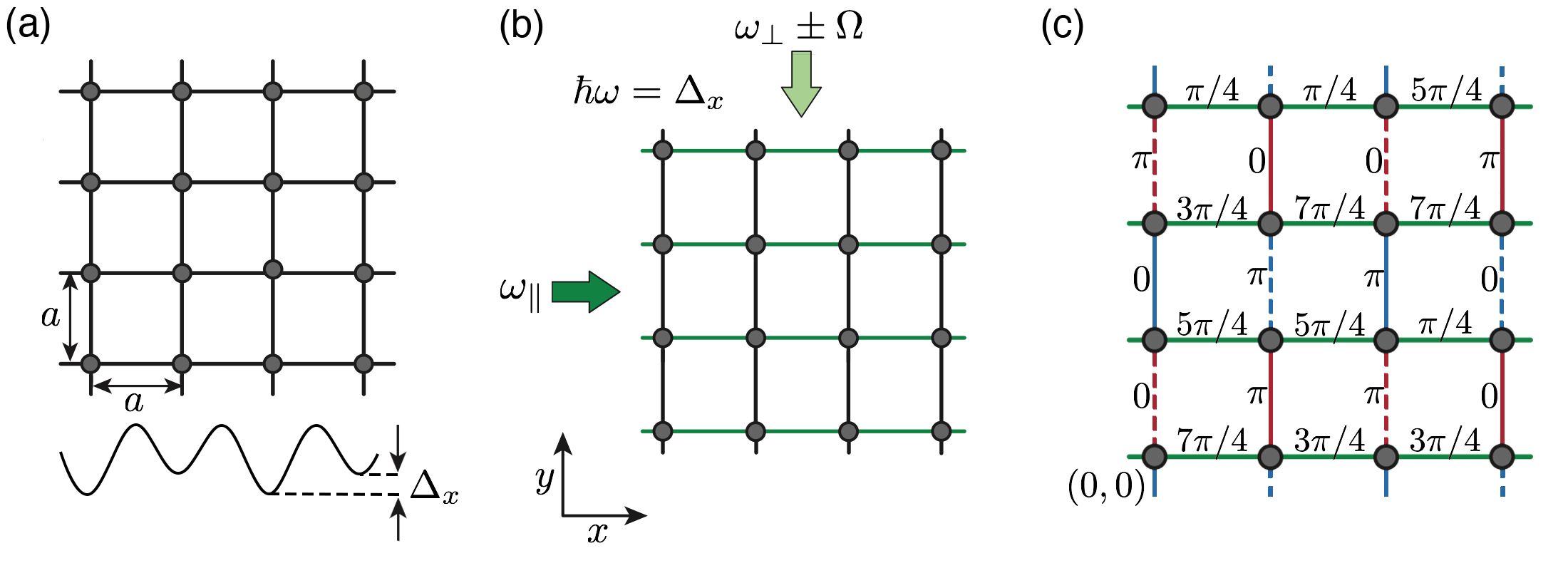
Figure S4: Second part of the experimental setup, where (a) the bosonic hopping $J_{x}$ is suppressed by an overlaid staggered potential $\Delta_{x}$, and (b) a pair of running-wave beams are used to restore resonant tunneling. (c) Phase distribution of the final effective Hamiltonian, realizing a homogenous background flux $\Phi=\pi/2$.

References

Chen et al. (2010)Xie Chen, Zheng-Cheng Gu,
and Xiao-Gang Wen, “Local unitary
transformation, long-range quantum entanglement, wave function
renormalization, and topological order,” Phys.
Rev. B 82, 155138
(2010).
Chen et al. (2013)Xie Chen, Zheng-Cheng Gu,
Zheng-Xin Liu, and Xiao-Gang Wen, “Symmetry protected
topological orders and the group cohomology of their symmetry group,” Phys. Rev. B 87, 155114 (2013).
Lu and Vishwanath (2012)Yuan-Ming Lu and Ashvin Vishwanath, “Theory and classification of interacting integer topological phases in two
dimensions: A chern-simons approach,” Phys.
Rev. B 86, 125119
(2012).
Tsui et al. (1982)D. C. Tsui, H. L. Stormer, and A. C. Gossard, “Two-dimensional
magnetotransport in the extreme quantum limit,” Phys. Rev. Lett. 48, 1559–1562 (1982).
Laughlin (1983)R. B. Laughlin, “Anomalous
quantum hall effect: An incompressible quantum fluid with fractionally
charged excitations,” Phys. Rev. Lett. 50, 1395–1398 (1983).
Haldane (1983)F. D. M. Haldane, “Nonlinear field theory of large-spin heisenberg antiferromagnets:
Semiclassically quantized solitons of the one-dimensional easy-axis néel
state,” Phys. Rev. Lett. 50, 1153–1156 (1983).
Pollmann et al. (2010)Frank Pollmann, Ari M. Turner, Erez Berg, and Masaki Oshikawa, “Entanglement spectrum of a
topological phase in one dimension,” Phys.
Rev. B 81, 064439
(2010).
Vishwanath and Senthil (2013)Ashvin Vishwanath and T. Senthil, “Physics of
three-dimensional bosonic topological insulators: Surface-deconfined
criticality and quantized magnetoelectric effect,” Phys.
Rev. X 3, 011016
(2013).
Note (1)As well as putative spin liquid phases of frustrated
magnets.
Girvin and MacDonald (1987)S. M. Girvin and A. H. MacDonald, “Off-diagonal
long-range order, oblique confinement, and the fractional quantum hall
effect,” Phys. Rev. Lett. 58, 1252–1255 (1987).
Zhang et al. (1989)S. C. Zhang, T. H. Hansson,
and S. Kivelson, “Effective-field-theory model
for the fractional quantum hall effect,” Phys.
Rev. Lett. 62, 82–85
(1989).
Zhang (1992)Shou Cheng Zhang, “The
chern–simons–landau–ginzburg theory of the fractional quantum hall
effect,” International Journal of Modern Physics B 6, 25–58 (1992).
Greschner et al. (2014a)Sebastian Greschner, Luis Santos, and Dario Poletti, “Exploring Unconventional Hubbard Models with Doubly Modulated Lattice
Gases,” Physical Review Letters 113, 183002 (2014a).
Di Liberto et al. (2014)Marco Di Liberto, Charles E Creffield, GI Japaridze, and C Morais Smith, “Quantum simulation of correlated-hopping models with fermions in optical
lattices,” Physical Review A 89, 013624 (2014).
Hudomal et al. (2020)Ana Hudomal, Ivana Vasić, Nicolas Regnault, and Zlatko Papić, “Quantum scars
of bosons with correlated hopping,” Communications Physics 3, 99 (2020).
Lienhard et al. (2020)Vincent Lienhard, Pascal Scholl, Sebastian Weber, Daniel Barredo,
Sylvain de Léséleuc, Rukmani Bai, Nicolai Lang, Michael Fleischhauer, Hans Peter Büchler, Thierry Lahaye, et al., “Realization of a density-dependent peierls phase in a synthetic, spin-orbit
coupled rydberg system,” Physical Review X 10, 021031 (2020).
Chu et al. (2023)Anjun Chu, Asier Piñeiro Orioli, Diego Barberena, James K Thompson, and Ana Maria Rey, “Photon-mediated correlated hopping in a synthetic ladder,” Physical Review Research 5, L022034 (2023).
He et al. (2015a)Yin-Chen He, Subhro Bhattacharjee, R. Moessner, and Frank Pollmann, “Bosonic
integer quantum hall effect in an interacting lattice model,” Phys. Rev. Lett. 115, 116803 (2015a).
Fuji et al. (2016)Yohei Fuji, Yin-Chen He,
Subhro Bhattacharjee, and Frank Pollmann, “Bridging coupled wires and
lattice hamiltonian for two-component bosonic quantum hall states,” Phys. Rev. B 93, 195143 (2016).
Liu et al. (2019)Wanli Liu, Zhiyu Dong,
Zhihuan Dong, Chenrong Liu, Wei Yan, and Yan Chen, “Bosonic Integer Quantum Hall States without Landau
Levels on Square Lattice,” Physical Review B 99, 085305 (2019), arxiv:1712.01212 .
Regnault and Bernevig (2011)Nicolas Regnault and B Andrei Bernevig, “Fractional
chern insulator,” Physical Review X 1, 021014 (2011).
Murthy and Shankar (2012)Ganpathy Murthy and R Shankar, “Hamiltonian theory of fractionally filled chern bands,” Physical Review B 86, 195146 (2012).
Zhao et al. (2021)YX Zhao, Cong Chen,
Xian-Lei Sheng, and Shengyuan A Yang, “Switching spinless and
spinful topological phases with projective p t symmetry,” Physical Review Letters 126, 196402 (2021).
Chen et al. (2012)Gang Chen, Andrew Essin, and Michael Hermele, “Majorana spin liquids and
projective realization of su (2) spin symmetry,” Physical Review B 85, 094418 (2012).
Liu and Bergholtz (2022)Zhao Liu and Emil J Bergholtz, “Recent
developments in fractional chern insulators,” arXiv preprint arXiv:2208.08449 (2022).
Lin et al. (2023)Yu-Ping Lin, Chunxiao Liu, and Joel E Moore, “Complex magnetic and spatial
symmetry breaking from correlations in kagome flat bands,” arXiv preprint arXiv:2307.11810 (2023).
Greschner et al. (2014b)S. Greschner, G. Sun,
D. Poletti, and L. Santos, “Density-dependent synthetic gauge fields
using periodically modulated interactions,” Phys. Rev. Lett. 113, 215303 (2014b).
Dunlap and Kenkre (1986)D. H. Dunlap and V. M. Kenkre, “Dynamic
localization of a charged particle moving under the influence of an electric
field,” Physical Review B 34, 3625–3633 (1986).
Aidelsburger et al. (2011)M. Aidelsburger, M. Atala,
S. Nascimbène, S. Trotzky, Y.-A. Chen, and I. Bloch, “Experimental realization of strong effective magnetic
fields in an optical lattice,” Phys. Rev. Lett. 107, 255301 (2011).
Struck et al. (2012)J. Struck, C. Ölschläger, M. Weinberg, P. Hauke,
J. Simonet, A. Eckardt, M. Lewenstein, K. Sengstock, and P. Windpassinger, “Tunable Gauge Potential for Neutral and
Spinless Particles in Driven Optical Lattices,” Physical Review Letters 108, 225304 (2012).
Jiménez-García et al. (2012)K. Jiménez-García, L. J. LeBlanc, R. A. Williams, M. C. Beeler, A. R. Perry, and I. B. Spielman, “Peierls Substitution in an Engineered Lattice Potential,” Physical Review Letters 108, 225303 (2012).
Jotzu et al. (2014)Gregor Jotzu, Michael Messer,
Rémi Desbuquois,
Martin Lebrat, Thomas Uehlinger, Daniel Greif, and Tilman Esslinger, “Experimental realization of the
topological Haldane model with ultracold fermions,” Nature 515, 237–240 (2014).
Hauschild and Pollmann (2018)Johannes Hauschild and Frank Pollmann, “Efficient numerical simulations with Tensor Networks: Tensor Network Python
(TeNPy),” SciPost Phys. Lect. Notes , 5 (2018).
Miao et al. (2022)Shiwan Miao, Zhongchi Zhang,
Yajuan Zhao, Zihan Zhao, Huaichuan Wang, and Jiazhong Hu, “Bosonic fractional quantum Hall conductance in shaken
honeycomb optical lattices without flat bands,” Physical Review B 106, 054310 (2022).
He et al. (2015b)Yin-Chen He, Subhro Bhattacharjee, Frank Pollmann, and R. Moessner, “Kagome chiral
spin liquid as a gauged symmetry protected topological phase,” Phys. Rev. Lett. 115, 267209 (2015b).
Barkeshli et al. (2015)M Barkeshli, NY Yao, and CR Laumann, “Continuous preparation of a
fractional chern insulator,” Physical review letters 115, 026802 (2015).
Motruk and Pollmann (2017)Johannes Motruk and Frank Pollmann, “Phase transitions and adiabatic preparation of a fractional chern insulator
in a boson cold-atom model,” Physical Review B 96, 165107 (2017).
Goldman et al. (2014)Nathan Goldman, G Juzeliūnas, Patrik Öhberg, and Ian B Spielman, “Light-induced
gauge fields for ultracold atoms,” Reports on Progress in Physics 77, 126401 (2014).
Dalibard (2015)Jean Dalibard, “Introduction
to the physics of artificial gauge fields,” Quantum Matter at Ultralow Temperatures
(2015).
Zhai (2015)Hui Zhai, “Degenerate quantum
gases with spin–orbit coupling: a review,” Reports on Progress in Physics 78, 026001 (2015).
Goldman et al. (2016)Nathan Goldman, Jan C Budich,
and Peter Zoller, “Topological quantum matter
with ultracold gases in optical lattices,” Nature Physics 12, 639–645 (2016).
Cooper et al. (2019)NR Cooper, J Dalibard, and IB Spielman, “Topological bands for
ultracold atoms,” Reviews of modern physics 91, 015005 (2019).
Yao et al. (2013)Norman Y Yao, Alexey V Gorshkov, Chris R Laumann, Andreas M Läuchli, Jun Ye, and Mikhail D Lukin, “Realizing fractional chern insulators in dipolar spin systems,” Physical review
letters 110, 185302
(2013).
Cesa and Martin (2013)Alexandre Cesa and John Martin, “Artificial abelian gauge potentials induced by dipole-dipole interactions
between rydberg atoms,” Physical Review A 88, 062703 (2013).
Wu et al. (2022)Xiaoling Wu, Fan Yang, Shuo Yang,
Klaus Mølmer, Thomas Pohl, Meng Khoon Tey, and Li You, “Manipulating synthetic gauge fluxes via multicolor
dressing of rydberg-atom arrays,” Physical Review Research 4, L032046 (2022).
Celi et al. (2014)Alessio Celi, Pietro Massignan, Julius Ruseckas, Nathan Goldman, Ian B Spielman, G Juzeliūnas, and M Lewenstein, “Synthetic
gauge fields in synthetic dimensions,” Physical review letters 112, 043001 (2014).
Senthil et al. (2004)T. Senthil, Leon Balents,
Subir Sachdev, Ashvin Vishwanath, and Matthew P. A. Fisher, “Quantum criticality beyond the
landau-ginzburg-wilson paradigm,” Phys.
Rev. B 70, 144407
(2004).
Xu and Senthil (2013)Cenke Xu and T. Senthil, “Wave functions of bosonic
symmetry protected topological phases,” Phys.
Rev. B 87, 174412
(2013).
Liu et al. (2014)Zheng-Xin Liu, Zheng-Cheng Gu, and Xiao-Gang Wen, “Microscopic realization of two-dimensional bosonic topological
insulators,” Phys. Rev. Lett. 113, 267206 (2014).
Goldman and Dalibard (2014)Nathan Goldman and Jean Dalibard, “Periodically
driven quantum systems: effective hamiltonians and engineered gauge
fields,” Physical review X 4, 031027 (2014).
Bukov et al. (2016)Marin Bukov, Markus Heyl,
David A. Huse, and Anatoli Polkovnikov, “Heating and many-body
resonances in a periodically driven two-band system,” Physical Review B 93, 155132 (2016).
Kuwahara et al. (2016)Tomotaka Kuwahara, Takashi Mori, and Keiji Saito, “Floquet–magnus theory and generic transient dynamics in periodically driven
many-body quantum systems,” Annals of Physics 367, 96–124 (2016).
Mori et al. (2016)Takashi Mori, Tomotaka Kuwahara, and Keiji Saito, “Rigorous bound on
energy absorption and generic relaxation in periodically driven quantum
systems,” Physical review letters 116, 120401 (2016).
Abanin et al. (2017)Dmitry Abanin, Wojciech De Roeck, Wen Wei Ho,
and François Huveneers, “A rigorous
theory of many-body prethermalization for periodically driven and closed
quantum systems,” Communications in Mathematical Physics 354, 809–827 (2017).
Weidinger and Knap (2017)Simon A Weidinger and Michael Knap, “Floquet
prethermalization and regimes of heating in a periodically driven,
interacting quantum system,” Scientific reports 7, 45382 (2017).
Machado et al. (2019)Francisco Machado, Gregory D Kahanamoku-Meyer, Dominic V Else, Chetan Nayak, and Norman Y Yao, “Exponentially slow heating in short and long-range interacting floquet
systems,” Physical Review Research 1, 033202 (2019).
Fuji and Furusaki (2019)Yohei Fuji and Akira Furusaki, “Quantum hall
hierarchy from coupled wires,” Phys. Rev. B 99, 035130 (2019).
(61)For additional details on the perturbative
coupled-wire analysis and numerical simulations, please see the Supplementary
Materials.
Wen (1995)Xiao-Gang Wen, “Topological orders and edge excitations in fractional quantum hall
states,” Adv. Phys. 44, 405–473 (1995).
He et al. (2014)Yin-Chen He, D. N. Sheng, and Yan Chen, “Obtaining
topological degenerate ground states by the density matrix renormalization
group,” Phys. Rev. B 89, 075110 (2014).
Grushin et al. (2015)Adolfo G. Grushin, Johannes Motruk, Michael P. Zaletel, and Frank Pollmann, “Characterization and stability of a fermionic
fractional chern insulator,” Phys. Rev. B 91, 035136 (2015).
Sterdyniak et al. (2015)A Sterdyniak, Nigel R Cooper, and N Regnault, “Bosonic
integer quantum hall effect in optical flux lattices,” Physical Review Letters 115, 116802 (2015).
He et al. (2017)Yin-Chen He, Fabian Grusdt, Adam Kaufman,
Markus Greiner, and Ashvin Vishwanath, “Realizing and adiabatically
preparing bosonic integer and fractional quantum hall states in optical
lattices,” Physical Review B 96, 201103 (2017).
Dalibard et al. (2011)Jean Dalibard, Fabrice Gerbier, Gediminas Juzeliūnas, and Patrik Öhberg, “Colloquium: Artificial gauge potentials for neutral atoms,” Reviews of Modern Physics 83, 1523 (2011).
Aidelsburger et al. (2015a)Monika Aidelsburger, Michael Lohse, Christian Schweizer, Marcos Atala, Julio T Barreiro, Sylvain Nascimbène, NR Cooper, Immanuel Bloch, and Nathan Goldman, “Measuring the
chern number of hofstadter bands with ultracold bosonic atoms,” Nature Physics 11, 162–166 (2015a).
Tai et al. (2017)M Eric Tai, Alexander Lukin,
Matthew Rispoli, Robert Schittko, Tim Menke, Dan Borgnia, Philipp M Preiss, Fabian Grusdt, Adam M Kaufman, and Markus Greiner, “Microscopy of the interacting harper–hofstadter model in the two-body
limit,” Nature 546, 519–523 (2017).
Barbiero et al. (2019)Luca Barbiero, Christian Schweizer, Monika Aidelsburger, Eugene Demler, Nathan Goldman, and Fabian Grusdt, “Coupling
ultracold matter to dynamical gauge fields in optical lattices: From flux
attachment to z2 lattice gauge theories,” Science advances 5, eaav7444 (2019).
Impertro et al. (2023)Alexander Impertro, Simon Karch, Julian F. Wienand, SeungJung Huh, Christian Schweizer, Immanuel Bloch, and Monika Aidelsburger, “Local readout and control of current and kinetic energy operators in
optical lattices,” (2023), arXiv:2312.13268 [cond-mat.quant-gas]
.
Jaksch and Zoller (2003)Dieter Jaksch and Peter Zoller, “Creation of
effective magnetic fields in optical lattices: the hofstadter butterfly for
cold neutral atoms,” New Journal of Physics 5, 56 (2003).
Aidelsburger et al. (2015b)Monika Aidelsburger, Michael Lohse, C Schweizer,
Marcos Atala, Julio T Barreiro, S Nascimbene, NR Cooper, Immanuel Bloch, and N Goldman, “Measuring the chern number of hofstadter bands with ultracold bosonic
atoms,” Nature
Physics 11, 162–166
(2015b).
Miyake et al. (2013)Hirokazu Miyake, Georgios A Siviloglou, Colin J Kennedy, William Cody Burton, and Wolfgang Ketterle, “Realizing the harper hamiltonian with laser-assisted tunneling in optical
lattices,” Physical review letters 111, 185302 (2013).
Aidelsburger et al. (2013)M. Aidelsburger, M. Atala,
M. Lohse, J. T. Barreiro, B. Paredes, and I. Bloch, “Realization of the hofstadter hamiltonian with ultracold
atoms in optical lattices,” Phys. Rev. Lett. 111, 185301 (2013).
Supplementary Information:

References

Fuji et al. (2016)Yohei Fuji, Yin-Chen He,
Subhro Bhattacharjee, and Frank Pollmann, “Bridging coupled wires and
lattice hamiltonian for two-component bosonic quantum hall states,” Phys. Rev. B 93, 195143 (2016).
Giamarchi (2003)Thierry Giamarchi, Quantum Physics in
One Dimension (Oxford University Press, New York, 2003).
Kane et al. (2002)C. L. Kane, Ranjan Mukhopadhyay, and T. C. Lubensky, “Fractional quantum hall effect in an array of quantum wires,” Phys. Rev. Lett. 88, 036401 (2002).
Teo and Kane (2014)Jeffrey C. Y. Teo and C. L. Kane, “From
luttinger liquid to non-abelian quantum hall states,” Phys.
Rev. B 89, 085101
(2014).
Lu and Vishwanath (2012)Yuan-Ming Lu and Ashvin Vishwanath, “Theory and classification of interacting integer topological phases in two
dimensions: A chern-simons approach,” Phys.
Rev. B 86, 125119
(2012).
Wen (1995)Xiao-Gang Wen, “Topological orders and edge excitations in fractional quantum hall
states,” Adv. Phys. 44, 405–473 (1995).
Mross et al. (2017)David F. Mross, Jason Alicea, and Olexei I. Motrunich, “Symmetry and
duality in bosonization of two-dimensional dirac fermions,” Phys. Rev. X 7, 041016 (2017).
Fuji and Furusaki (2019)Yohei Fuji and Akira Furusaki, “Quantum hall
hierarchy from coupled wires,” Phys. Rev. B 99, 035130 (2019).
Hauschild and Pollmann (2018)Johannes Hauschild and Frank Pollmann, “Efficient numerical simulations with Tensor Networks: Tensor Network Python
(TeNPy),” SciPost Phys. Lect. Notes , 5 (2018).
Aidelsburger (2015)Monika Aidelsburger, Artificial gauge
fields with ultracold atoms in optical lattices (Springer, 2015).