Deconfined Fermi liquid to Fermi liquid transition and superconducting instability

Abstract

Deconfined quantum critical points (DQCP) have attracted lots of attentions in the past decades, but were mainly restricted to incompressible phases. On the other hand, various experimental puzzles call for new theory of unconventional quantum criticality between metals at a generic density. Here we explore the possibility of a deconfined transition between two symmetric Fermi liquids in a bilayer model tuned by inter-layer antiferromagnetic spin-spin coupling $J_{\perp}$. Across the transition the Fermi surface volume per flavor jumps by $1/2$ of the Brillouin zone (BZ), similar to the small to large Fermi surface transitions in heavy Fermion systems and maybe also in the high Tc cuprates. But in the bilayer case the small Fermi surface phase (dubbed as sFL) has neither symmetry breaking nor fractionalization, akin to the symmetric mass generation (SMG) discussed in high energy physics. We formulate a deconfined critical theory where the two Fermi liquids correspond to higgs and/or confined phases of a $U(1)\times U(1)$ gauge theory. We show that this deconfined FL to FL transition (DFFT) fixed point is unstable to pairing and thus a superconductor dome is expected at low temperature. At finite temperature above the pairing scale, microscopic electron is a three particle bound state of the deconfined fractional fermions in the critical theory. We also introduce another parameter which can suppress the pairing instability, leading to a deconfined tri-critical point stable to zero temperature. We also provide numerical results of the bilayer model in one dimension, with a Luther-Emery liquid between two different Luttinger liquids, similar to the phase diagram from the field theory in two dimension. Our work opens a new direction to exploring deconfined metallic criticality and new pairing mechanism from critical gauge field.

I Introduction

There have been intensive studies on possible unconventional transitions beyond the familiar Landau-Ginzburg framework based on symmetry breaking order parameters. One famous example is the deconfined quantum critical point (DQCP)[1, 2] between the Neel ordered and valence bond solid (VBS) phases on square lattice. DQCP was also suggested for symmetric mass generation (SMG)[3, 4] transition between a semimetal and an insulator[5]. In these examples the two sides of the phase transitions are just conventional phases without any fractionalization, but the critical regime is described by fractionalized particle and emergent internal gauge field at low energy. So far the discussions of deconfined criticalities are largely restricted to insulators or semimetals at integer filling. On the other hand, experiments in the heavy fermion systems[6, 7, 8, 9, 10, 11, 12, 13] and in the high temperature superconductor cuprates[14, 15, 16, 17] suggest the possibility of a quantum critical point with Fermi surface volume jump between two metallic phases. Besides, the phenomenology seems to be beyond the conventional metallic criticality simply with a fluctuating symmetry breaking order parameter such as in the Hertz-Millis-Moriya theory[18, 19, 11]. Therefore it is important to generalize the idea of DQCP to the more sophisticated phase transition with Fermi surfaces in the two sides. Critical theories have been proposed for the unusual case where one side has a neutral Fermi surface[20, 21], but the examples are essentially Mott or orbital-selective Mott transition with the volume of the critical Fermi surface fixed at the half filling. A DQCP with both sides as conventional metallic phases with arbitrary size of Fermi surfaces is still elusive, despite of some progress for a deconfined metallic transition with an onset of antiferromagnetism[22].

In this work we turn to a different setup with a bilayer model and identify a much cleaner small to large Fermi surface transition with symmetric Fermi liquids in both sides. More specifically, we consider a bilayer Hubbard or t-J model with strong inter-layer spin-spin interaction $J_{\perp}$, but no inter-layer hopping $t_{\perp}$. Naively this seems impossible because usually $J_{\perp}$ is generated from the $t^{2}_{\perp}/U$ super-exchange process. But it is actually possible to generate a large $J_{\perp}$ from Hund’s coupling to a rung-singlet from a different orbital as proposed by one of us for the recently found nickelate superconductor[23, 24, 25, 26, 27]. In this situation, the symmetry is $(U(1)_{t}\times U(1)_{b}\times SU(2))/Z_{2}$ with the two U(1) corresponding to the charge conservations of the top and bottom layers respectively. Oshikawa’s non-perturbative proof of the Luttinger theorem[28] then shows that there are two classes of symmetric and featureless Fermi liquids: a conventional Fermi liquid (FL) and a second Fermi liquid (sFL)[30, 26]. The sFL phase has Fermi surface volume smaller than the FL phase by 1/2 of the Brillouin zone (BZ) per flavor. At a fixed density per layer $n=1-x$ with small hole doping level $x$, we have a FL phase with large Fermi surface volume $A_{FS}=\frac{1-x}{2}$ per flavor at small $J_{\perp}$. Then in the large $J_{\perp}$ regime, the sFL phase with $A_{FS}=-\frac{x}{2}$ is stabilized instead. Therefore there is a large to small Fermi surface transition tuned by $J_{\perp}$. The sFL phase is clearly beyond any weak coupling theory and it arises only in the strong coupling regime of the four fermion interaction $J_{\perp}$ akin to the symmetric mass generation[5, 31] discussed in the high energy physics, though in our case the charge carriers are only partially gapped.

The FL to sFL transition, if continuous, must be beyond Landau-Ginzburg framework as there is no symmetry breaking order parameter. Meanwhile both phases are conventional without fractionalization. Thus it is natural to expect a deconfined criticality similar to the Neel to VBS DQCP. We formulate such a theory in this work. In our critical theory, the two phases correspond to higgsed and/or confined phases of a U(1)$\times$ U(1) gauge theory with deconfined fractionalized particle existing only at the critical regime. The critical theory is unstable to pairing at zero temperature, but the pairing scale can be suppressed to be arbitrarily low due to the almost balance between the repulsive and attractive interaction from the two U(1) gauge fields. Similar features of balance from two gauge fields have been discussed previously in other contexts[32, 22, 33, 34]. Above the pairing energy scale, we have a large critical regime where electron is a three particle bound state of the elementary fermions in the low energy theory. One immediate implication is that the quasiparticle residue $Z$ vanishes at the critical regime and any single electron spectroscopy measurement (such as ARPES or STM) can not see any coherent quasiparticle. We also include another axis to tune $\delta U$, the difference between the intra-layer and inter-layer repulsion. We argue that the pairing instability can be suppressed by tuning $\delta U$ and there is a stable deconfined tri-critical point down to zero temperature, which separates a sFL phase, a FL phase, a superconductor phase and a deconfined metal (DM) phase which can be roughly understood as a stable phase similar to the deconfined critical regime.

Our work opens a door to study DQCP between compressible phases, which, unlike the previous discussions in insulators or semimetals, can arise at any electron density. We also provide numerical results from density matrix renormalization group (DMRG) in one dimension, which supports the existence of the small and large Fermi surface phases in the two sides and a Luther-Emery liquid in between. The Luther-Emery liquid has power law correlation of the inter-layer pairing between the two nearest neighbor sites. The pairing is remarkable given that the model has an infinite on-site inter-layer repulsive interaction. This is qualitatively in agreement with our field theory result of a superconductor dome at the critical region, indicating a new pairing mechanism associated with the small to large Fermi surface transition.

II One orbital bilayer Hubbard model

We consider the following one-orbital bilayer model:

$$H =-t\sum_{\langle ij\rangle}\sum_{\alpha}c^{\dagger}_{i;\alpha}c_{j;\alpha}+\frac{1}{2}U_{0}\sum_{i}\sum_{a=t,b}n^{2}_{i;a}$$ (1)

$$+V_{0}\sum_{i}n_{i;t}n_{i;b}+J_{\perp}\sum_{i}\vec{S}_{i;t}\cdot\vec{S}_{i;b}.$$

We view layer as a pseudospin, then we have four flavors labeled as $\alpha=a,\sigma$. $a=t,b$ labels the top and bottom layer while $\sigma=\uparrow,\downarrow$ labels the spin. $n_{i;t}$ and $n_{i;b}$ indicate the density at site $i$ for the top and bottom layers respectively. $\vec{S}_{i;t}$ and $\vec{S}_{i;b}$ are the spin operators in the two layers. If $V_{0}=U_{0}$ and $J_{\perp}=0$, this is the SU(4) Hubbard model. Generally $U_{0}$ and $V_{0}$ can be different and the model can be rewritten as:

$$H =-t\sum_{\langle ij\rangle}\sum_{\alpha}c^{\dagger}_{i;\alpha}c_{j;\alpha}+\frac{1}{2}U\sum_{i}n_{i}^{2}$$ (2)

$$+\delta U\sum_{i}P_{i;z}^{2}+J_{\perp}\sum_{i}\vec{S}_{i;t}\cdot\vec{S}_{i;b},$$

where $n_{i}=n_{i;t}+n_{i;b}$ and $P_{i;z}=n_{i;t}-n_{i;b}$. We have $U=\frac{1}{2}\left(U_{0}+V_{0}\right)$ and $\delta U=\frac{1}{4}\left(U_{0}-V_{0}\right)$. The model has a $\left(U(1)_{t}\times U(1)_{b}\times SU(2)\right)/Z_{2}$ symmetry with $U(1)$ charge conservation in the two layers separately because there is no $t_{\perp}$ hopping. We have electron density(summed over spin) per layer to be $n_{t}=n_{b}=1-x$ per site. So the filling per spin per layer is $\nu=\frac{1-x}{2}$.

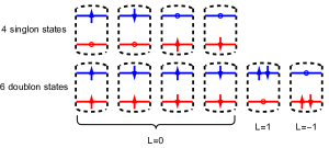
Figure 1: Restricted Hilbert space at each site in the large $U$ regime. The dashed box represents a single site. Blue lines and red lines represent top and bottom layers respectively. The empty state is penalized by the large $U$ and there are 4 singlon states and 6 doublon states. The last 2 doublon states are further penalized by $\delta U$ and should be removed if we also take the large $\delta U$ limit.

We are interested in the large $U_{0}$ and $V_{0}$ regime in this work with $U_{0}>V_{0}\gg t,J_{\perp}$. Note that the electron density summed over two layers and spin is $n_{T}=2(1-x)$. $n_{T}=1$ corresponds to the Mott insulator and we consider the regime $1<n_{T}<2$. The restricted Hilbert space due to the large U is shown in Fig. (1) which consists of 4 singlon states (with $n_{T}=1$) and 6 doublon states (with $n_{T}=2$). The empty state is forbidden since we need to add one more doubly occupied site to create one empty site, which costs energy $U_{0}$ or $V_{0}$. The Hamiltonian in this restricted Hilbert space now becomes[30]

$$H =-t\sum_{\langle ij\rangle}\sum_{\alpha}P_{4+6}c^{\dagger}_{i;\alpha}c_{j;\alpha}P_{4+6}$$ (3)

$$+J_{\perp}\sum_{i}\vec{S}_{i;t}\cdot\vec{S}_{i;b}+\delta U\sum_{i}P_{i;z}^{2}+...,$$

where $P_{4+6}$ is the projection operator into the 4-singlon-6-doublon Hilbert space shown in Fig. 1. Note that here we include the intra-layer spin-spin coupling in the $...$ term.

If we further take the limit that $\delta U$ is also large, the last two doublon states in Fig. (1) are also forbidden. Then the restricted Hilbert space on each site now has 4 single occupied states and 4 double occupied states. The Hamiltonian in this restricted Hilbert space simply consists of $t$ and $J_{\perp}$ term:

$$H =-t\sum_{\langle ij\rangle}\sum_{\alpha}P_{4+4}c^{\dagger}_{i;\alpha}c_{j;\alpha}P_{4+4}$$ (4)

$$+J_{\perp}\sum_{i}\vec{S}_{i;t}\cdot\vec{S}_{i;b}+...,$$

where $P_{4+4}$ is the projection operator into the 4-singlon-4-doublon Hilbert space. Again we include the intra-layer Heisenberg spin-spin coupling in the $...$ term.

II.1 Relation to the bilayer nickelate

The model in Eq. 1 is unusual in the sense that there is a $J_{\perp}$, but no inter-layer hopping $t_{\perp}$. As usually spin-spin coupling is from second order super-exchange process with $J_{\perp}\sim\frac{t_{\perp}^{2}}{U}$, it is not clear that the model is physical. The model has been discussed by one of us in the context of graphene moiré system[30] where the valley plays the role of the layer and the $J_{\perp}$ term is from the phonon mediated anti-Hund’s coupling. The model was also proposed for bilayer optical lattice with strong inter-layer potential difference, though in a non-equilibrium setting[35].

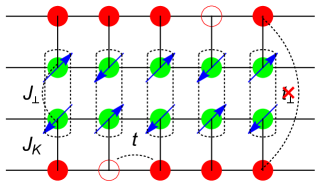
Figure 2: Illustration of the double Kondo model for the bilayer nickelate. The solid green circle with arrow, solid red circle, and the red circle correspond to the spin-$1/2$ moments, electron, and hole, respectively. $t$, $J_{\perp}$, $J_{K}$ are the hopping, inter-layer coupling and the Kondo coupling. There is no $t_{\perp}$ in this model. In the large $J_{\perp}$ limit, the spin moments form rung singlet $\frac{1}{\sqrt{2}}(\ket{\uparrow\downarrow}-\ket{\downarrow\uparrow})$.

More recently a more realistic realization of the model has been proposed[23, 24, 25, 26, 27] for the recently found nickelate superconductor La₃Ni₂O₇ under pressure with $n_{t}=n_{b}=1-x$ and $x\approx 0.5$. The key is to have additional spin moments forming bilayer rung singlet. Then the itinerant electron couples to the these spin moments through Hund’s coupling or super-exchange coupling $J_{K}$, which shares the strong $J_{\perp}$ of the spin moments to the itinerant electron. In the end the itinerant electron feels a strong $J_{\perp}$, but without $t_{\perp}$ as shown in Fig. 2.

In this situation one expect that $V_{0}\ll U_{0}$ and $U_{0}\gg t$. In realistic system $V_{0}$ may not be too large, therefore one should also keep the empty state for each rung in the low energy Hilbert space, as is done in Ref. 26 by two of us. From our previous analysis at finite $V_{0}$, there are two different normal states: the conventional Fermi liquid and the second Fermi liquid (sFL) with Fermi surface volume smaller by 1/2 of the BZ per flavor. The sFL still satisfies Oshikawa’s non-perturbative proof of the Luttinger theorem, despite that it is beyond any weak coupling theory and is intrinsically strongly correlated. At low temperature, both the FL and sFL are unstable to superconductivity due to an attractive interaction mediated by an on-site virtual Cooper pair. In this work we are interested in the transition between the FL and the sFL phase, so we will make $V_{0}\rightarrow+\infty$ to suppress the pairing instability discussed in Ref. 26 completely.

II.2 sFL phase in the large $J_{\perp}$ limit

We consider the $U_{0},V_{0}\gg t$ limit and can then restrict to Eq. 4 or Eq. 3 depending on whether $\delta U$ is large or not. In either case, we expect two different metallic phases in the small and large $J_{\perp}$ regime at filling $n_{t}=n_{b}=1-x$ with small $x$. When $J_{\perp}$ is small, one can expect a conventional Fermi liquid phase with Fermi surface volume $A_{FS}=\frac{1-x}{2}$ per flavor.

In the large $J_{\perp}$ limit, the doublon state is dominated by the spin-singlet. We can label this S=0 doublon as $\ket{b}=b^{\dagger}_{i}\ket{0}$ with $\ket{0}$ as the empty state. Together with four singlon states $\ket{a\sigma}=f^{\dagger}_{i;a\sigma}\ket{0}$, we reach a SU(4) t-J model with $4+1=5$ states per site. The t-J model is written as:

$$H=-t\sum_{\langle ij\rangle}\sum_{\alpha}P_{4+1}c^{\dagger}_{i;\alpha}c_{j;\alpha}P_{4+1}+...,$$ (5)

We can then do the standard slave boson theory[14] for this usual t-J model: $c_{i;a\sigma}=(-1)^{\eta_{\sigma}}\frac{1}{\sqrt{2}}f^{\dagger}_{\bar{a}\bar{\sigma}}b_{i}$ where $\eta_{\uparrow}=-\eta_{\downarrow}=1$. We have the density $n_{f}=2x$ and $n_{b}=1-2x$. In terms of the parton construction, the model can be written as:

$$H=\frac{t}{2}\sum_{\langle ij\rangle}\sum_{\alpha}f^{\dagger}_{j;\alpha}f_{i;\alpha}b^{\dagger}_{i}b_{j}.$$ (6)

As usual, we can describe a Fermi liquid with condensation of the slave boson: $\langle b\rangle\neq 0$. Because $n_{f}=2x$ and each of the four flavor has filling $\frac{x}{2}$, we reach a Fermi surface volume of $A_{FS}=-\frac{x}{2}$, where the minus sign indicates that we have hole pocket because $c_{i}\sim f_{i}^{\dagger}$ and $f_{i}$ should be interpreted as annihilation of the hole. Also the small Fermi surface should center at $\mathbf{k}=(\pi,\pi)$ due to the negative hopping of $f$. One can see now we have a different Fermi liquid in the infinite $J_{\perp}$ limit with Fermi surface volume smaller than the non-interacting limit by 1/2 of the BZ per flavor. We dub this phase as the sFL phase[26]. Our goal is to formulate a theory for the potential large to small Fermi surface transition by tuning $J_{\perp}$ at a fixed $x$.

III Deconfined Fermi liquid to Fermi liquid transition in the large $\delta U$ limit

We first formulate a critical theory for the FL to sFL transition in the large $\delta U$ limit, so we can restrict to the model in Eq. 4. To capture the transition, we first need a unified framework to describe both the FL and the sFL phase. This can be done by a parton construction with a U(1)$\times$ U(1) gauge structure.

III.1 Parton construction

We introduce the standard Abrikosov fermion to represent the 4 singlon states: $f^{\dagger}_{i;a\sigma}\ket{0}$ with $a=t,b$. For the 4 doublon states, we introduce another fermion $\psi$ and $\psi^{\dagger}_{i;t\sigma}\psi^{\dagger}_{i;b\sigma^{\prime}}\ket{0}$ are 4 doublon states with $\sigma,\sigma^{\prime}=\uparrow,\downarrow$. Here $\psi_{i;a\sigma}$ annihilate a fermion at layer $a=t,b$ with spin $\sigma=\uparrow,\downarrow$ just as $f_{i;a\sigma}$. The electron operator projected to this Hilbert space is

$$c_{i;a\sigma}=\sum_{\sigma^{\prime}}f^{\dagger}_{i;\bar{a}\sigma^{\prime}}\psi_{i;\bar{a}\sigma^{\prime}}\psi_{i;a\sigma}.$$ (7)

where $\bar{a}$ is the opposite layer of $a$.

We have two local constraints: (I) $n_{i;f}+\frac{1}{2}\left(n_{i;\psi_{t}}+n_{i;\psi_{b}}\right)=1$ and (II) $n_{i;\psi_{t}}=n_{i;\psi_{b}}$ on each site. They generate two internal U(1) gauge fields $a_{\mu}$ and $b_{\mu}$ whose time components impose these two constraints as lagrangian multipliers. On average, we have density $n_{f}=2x$ while $n_{\psi_{t}}=n_{\psi_{b}}=1-2x$. The total density of electrons is $n_{f}+n_{\psi_{t}}+n_{\psi_{b}}=2(1-x)=n_{T}$.

The physical electron operator Eq. (7) is invariant under the following two internal U(1) gauge transformations: (1) $\psi_{i}\rightarrow\psi_{i}e^{i\theta_{a}(i)}$ and $f_{i}\rightarrow f_{i}e^{i2\theta_{a}(i)}$ for the U(1) gauge field $a_{\mu}$ (the subscript $a$ stands for the gauge field, not the layer index); (2) $f_{i}\rightarrow f_{i}$, $\psi_{i;t}\rightarrow\psi_{i;t}e^{i\theta_{b}(i)}$, $\psi_{i;b}\rightarrow\psi_{i;b}e^{-i\theta_{b}(i)}$ for the U(1) gauge field $b_{\mu}$. Meanwhile there is a global U(1) symmetry transformation: $c_{i;a}\rightarrow c_{i;a}e^{i\theta_{c}(i)}$. We can assign the charge to $\psi$, so under this global U(1) transformation, $f\rightarrow f$,$\psi_{i;a}\rightarrow\psi_{i;a}e^{i\frac{1}{2}\theta_{c}(i)}$. We introduce a probing field $A_{\mu}$ for this U(1) global symmetry. Another global U(1) symmetry transformation corresponding to the layer polarization $P_{z}$ is: $c_{i;t}\rightarrow c_{i;t}e^{i\theta_{d}(i)}$, $c_{i;b}\rightarrow c_{i;b}e^{-i\theta_{d}(i)}$. We assign the charge to $f$, so under this global U(1) transformation, $\psi\rightarrow\psi$, $f_{i;t}\rightarrow f_{i;t}e^{i\theta_{d}(i)}$, $f_{i;b}\rightarrow f_{i;b}e^{-i\theta_{d}(i)}$. We also introduce a probing field $B_{\mu}$ for the layer U(1). In the end, we have $f_{t}$ couples to $2a_{\mu}+B_{\mu}$, $f_{b}$ couples to $2a_{\mu}-B_{\mu}$, $\psi_{t}$ couples to $\frac{1}{2}A_{\mu}+a_{\mu}+b_{\mu}$ and $\psi_{b}$ couples to $\frac{1}{2}A_{\mu}+a_{\mu}-b_{\mu}$.

Rewriting the Hamiltonian Eq. (4) in terms of the partons and do the mean-field decoupling, we can obtain the following two different possible mean field ansatz:

$$H^{(1)}_{\mathrm{MF}}=-\sum_{i}\sum_{a=t,b}\Phi_{a}f^{\dagger}_{i;a\sigma}\psi_{i;a\sigma}+\mathrm{h.c.},$$ (8)

$$H^{(2)}_{\mathrm{MF}}=-\Delta\sum_{i}\epsilon_{\sigma\sigma^{\prime}}\psi_{i;t\sigma}\psi_{i;b\sigma^{\prime}}+\mathrm{h.c.}.$$

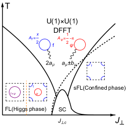
Figure 3: A schematic phase diagram with $J_{\perp}$, which tunes the mass of $\Phi_{a}$ and the temperature $T$ in the large $\delta U$ regime. In the FL phase, $\langle\Phi_{a}\rangle\neq 0$ and $\Delta=0$. When $\langle\Phi_{a}\rangle$ is large, $f$ and $\psi$ share a Fermi surface while when $\langle\Phi_{a}\rangle$ is small, $\psi$ has a Fermi surface around $\Gamma$ point and $f$ has a Fermi surface around $(\pi,\pi)$. In the sFL phase, $\langle\Phi_{a}\rangle=0$ and $\Delta\neq 0$. $\psi$ now is gapped while $f$ forms a small hole pocket. The two crossover boundaries are the usual V-shape quantum critical region for the critical boson $\Phi$. The dashed curve denote the pairing of $\psi$. The yellow dashed line denotes a Lifshitz transition within the FL phase. At low temperature, there is a superconductor dome due to the pairing instability of the DFFT fixed point. Above the pairing scale in the critical regime, we have two types of Fermi surfaces from $f$ and $\psi$ particles. Both of them couple to internal gauge field $a_{\mu},b_{\mu}$ and the electron is a three particle bound state $c\sim f^{\dagger}\psi\psi$ and thus there is no coherent single electron quasiparticle.

The variational parameters $\Phi_{a}$ and $\Delta$ need to be decided by optimizing the energy at each fixed $J_{\perp}$. Ideally this should be done through the variational Monte carlo (VMC) calculation because the simple self-consistent mean field analysis is known to be not trustable due to the constraint. Because our focus here is the universal theory of the transition, we leave the VMC calculation with detailed energetical analysis to future. Here we simply point out two different phases accessible in this parton framework:

• FL phase: $\Phi_{a}\neq 0,\Delta=0$. Now $f_{a}$ and $\psi_{a}$ hybridize and both of them can be identified as the electron operator $c_{a\sigma}\sim f_{a\sigma}\sim\psi_{a\sigma}$. The total density is $n_{T}=2-2x$ and the total Fermi surface volume per flavor is $\frac{1-x}{2}$ because we have four identical Fermi surfaces from the layer and spin. For the gauge field, $a_{\mu}$ is higgsed to be locked to $\frac{1}{2}A_{\mu}$ while $b_{\mu}$ is locked to $B_{\mu}$. This is a higgsed phase of the U(1)$\times$ U(1) gauge theory.

• sFL phase: $\Phi_{a}=0,\Delta\neq 0$ Now $\psi_{a}$ is gapped out because of the pairing. $a_{\mu}$ is higgsed to be locked to $-\frac{1}{2}A_{\mu}$ while $b_{\mu}$ is confined. In the end we have $c_{a\sigma}\sim f^{\dagger}_{\bar{a}\bar{\sigma}}$. $f$ couples to $-A_{\mu}$ and should be interpreted as the hole operator. Because $n_{f}=2x$, we expect Fermi surface volume $A_{FS}=-\frac{x}{2}$ per flavor.

Now we see that we can capture both the FL and the sFL phase within one framework. Although our formalism introduces $U(1)\times U(1)$ gauge field, the FL and sFL phases are conventional in the sense that the emergent gauge field is either higgsed or confined. Following our argument before, we naturally expect that the above two ansatz correspond to the small $J_{\perp}$ and the large $J_{\perp}$ regime. The next question is about the intermediate regime. In principle we can have an intermediate phase from the other two ansatz: (III) A superconductor phase with $\Phi_{a}\neq 0,\Delta\neq 0$ and (IV) A deconfined metal (DM) phase with $\Phi_{a}=0,\Delta=0$. Another possibility is a first order transition between the FL and the sFL phase directly. The most interesting possibility is a continuous direct transition from FL to sFL. If we start from the FL phase with finite $\Phi_{a}$, the question is whether the onset of the pairing $\Delta$ can coincide with the disappearance of the higgs condensation $\Phi_{a}$. In the mean field level this is impossible without fine tuning, but the gauge fluctuation can change the story completely. One famous example is the Neel to VBS DQCP[1] where the confinement happens immediately after the higgs phase is destroyed due to the proliferation of the monopole. In our case we will show a similar scenario with the onsets of the pairing driven by the destruction of the higgs condensation $\Phi_{a}$.

III.2 Critical theory

We start from the FL phase with $\langle\Phi_{a}\rangle\neq 0$, then we expect $\Phi_{a}$ decrease with $J_{\perp}$ because eventually we have the sFL phase with $\langle\Phi_{a}\rangle=0$ at large $J_{\perp}$. Next we will formulate a critical theory associated with the Higgs transition of $\Phi_{a}$ which vanishes at a critical value $J_{\perp}^{c}$. This critical theory can be described by the following Lagrangian:

$$\mathcal{L}_{\mathrm{c}}=\mathcal{L}_{\Phi}+\mathcal{L}_{f}+\mathcal{L}_{\psi},$$ (9)

where $\mathcal{L}_{\Phi}$ is

$$\mathcal{L}_{\Phi} =\bar{\Phi}_{t}\left(\partial_{\tau}-i\left(-\frac{A_{0}}{2}+B_{0}+a_{0}-b_{0}\right)\right)\Phi_{t}+\frac{1}{2m_{\Phi}}\bar{\Phi}_{t}\left(-i\vec{\nabla}-\left(-\frac{\vec{A}}{2}+\vec{B}+\vec{a}-\vec{b}\right)\right)^{2}\Phi_{t}$$ (10)

$$+\bar{\Phi}_{b}\left(\partial_{\tau}-i\left(-\frac{A_{0}}{2}-B_{0}+a_{0}+b_{0}\right)\right)\Phi_{b}+\frac{1}{2m_{\Phi}}\bar{\Phi}_{b}\left(-i\vec{\nabla}-\left(-\frac{\vec{A}}{2}-\vec{B}+\vec{a}+\vec{b}\right)\right)^{2}\Phi_{b}$$

$$-\mu_{\Phi}\left(\left|\Phi_{t}\right|^{2}+\left|\Phi_{b}\right|^{2}\right)+\lambda_{1}\left(\left|\Phi_{t}\right|^{2}+\left|\Phi_{b}\right|^{2}\right)^{2}+\lambda_{2}\left|\Phi_{t}\right|^{2}\left|\Phi_{b}\right|^{2}.$$

Here we assume that there is always a mirror reflection symmetry $\mathcal{M}$ which exchanges the two layers, so $\Phi_{a}$ and $\Phi_{b}$ have the same mass $\mu_{\Phi}$. $\mathcal{L}_{\Phi}$ is just the standard action for the Higgs transition. Here the boson fields $\Phi_{a},\Phi_{b}$ couples to the internal U(1) gauge fields $a_{\mu},b_{\mu}$ and also two probing fields $A_{\mu},B_{\mu}$. When $\mu_{\Phi}>0$, we have $\langle\Phi_{a}\rangle=\langle\Phi_{b}\rangle\neq 0$, which locks $a_{\mu}=\frac{1}{2}A_{\mu}$ and $b_{\mu}=B_{\mu}$. When $\mu_{\Phi}<0$, $\Phi_{a}$ is gapped and the two internal U(1) gauge fields $a_{\mu},b_{\mu}$ become alive.

$\mathcal{L}_{f}$ and $\mathcal{L}_{\psi}$ contain the action of the fermion $f$ and $\psi$:

$$\mathcal{L}_{f} =\bar{f}_{t;\sigma}\left(\partial_{\tau}-i\left(2a_{0}+B_{0}\right)\right)f_{t;\sigma}+\frac{1}{2m_{f}}\bar{f}_{t;\sigma}\left(-i\vec{\nabla}-\left(2\vec{a}+\vec{B}\right)\right)^{2}f_{t;\sigma}$$ (11)

$$+\bar{f}_{b;\sigma}\left(\partial_{\tau}-i\left(2a_{0}-B_{0}\right)\right)f_{b;\sigma}+\frac{1}{2m_{f}}\bar{f}_{b;\sigma}\left(-i\vec{\nabla}-\left(2\vec{a}-\vec{B}\right)\right)^{2}f_{b;\sigma}$$

$$-\mu_{f}\sum_{a=t,b}\bar{f}_{a;\sigma}f_{a;\sigma},$$

$$\mathcal{L}_{\psi} =\bar{\psi}_{t;\sigma}\left(\partial_{\tau}-i\left(\frac{A_{0}}{2}+a_{0}+b_{0}\right)\right)\psi_{t;\sigma}+\frac{1}{2m_{\psi}}\bar{\psi}_{t;\sigma}\left(-i\vec{\nabla}-\left(\frac{\vec{A}}{2}+\vec{a}+\vec{b}\right)\right)^{2}\psi_{t;\sigma}$$

$$+\bar{\psi}_{b;\sigma}\left(\partial_{\tau}-i\left(\frac{A_{0}}{2}+a_{0}-b_{0}\right)\right)\psi_{b;\sigma}+\frac{1}{2m_{\psi}}\bar{\psi}_{b;\sigma}\left(-i\vec{\nabla}-\left(\frac{\vec{A}}{2}+\vec{a}-\vec{b}\right)\right)^{2}\psi_{b;\sigma}$$

$$-\mu_{\psi}\sum_{a=t,b}\bar{\psi}_{a;\sigma}\psi_{a;\sigma}.$$

Remember that $f_{a}$ couples to $2a_{\mu}\pm B_{\mu}$ for $a=t,b$ and $\psi_{a}$ couples to $\frac{1}{2}A_{\mu}+a_{\mu}\pm b_{\mu}$ for $a=t,b$. In the higgs phase with $\langle\Phi_{a}\rangle\neq 0$, both $f_{a\sigma},\psi_{a\sigma}$ can be identified as electron operator. When $|\Phi_{a}|$ is large enough, $f,\psi$ hybridize together to form a single large Fermi surface. Then at small but finite $\Phi_{a}$, we expect separate Fermi surfaces dominated by $f$ and $\psi$. But their total Fermi surface volume is still $A_{FS}=\frac{1-x}{2}$ per flavor and it is still a conventional FL phase. When approaching the critical point $\mu_{\Phi}=0$, the quasi particle residue of both Fermi surfaces vanish. At the critical point, the Fermi surface volumes per flavor from $f$ and $\psi$ are $\frac{x}{2}$ and $\frac{1}{2}-x$ respectively. In principle that there should be a Yukawa coupling $\delta L=g\Phi f^{\dagger}_{a\sigma}\psi_{a\sigma}$. But given the mismatch of the Fermi surfaces from $f$ and $\psi$ in the momentum space, this coupling is irrelevant because the critical boson $\Phi$ is mainly at zero momentum.

When $\mu_{\Phi}<0$, $\Phi_{a}$ is gapped and we can ignore $\mathcal{L}_{\Phi}$. But now the two internal U(1) gauge fields $a_{\mu},b_{\mu}$ become alive and we need to decide whether the Fermi surfaces from $f$ and $\psi$ are stable to the gauge fluctuation or not. $f$ only couples to $2a_{\mu}$ and the physics is then similar to the familiar U(1) spin liquid with spinon Fermi surface. From the previous works we know that the Fermi surface from $f$ should be stable. On the other hand, $\psi_{t}$ and $\psi_{b}$ couple to $a_{\mu}$ with the same charge, but couple to $b_{\mu}$ with opposite charge. It is known that $b_{\mu}$ will mediate attractive interaction between $\psi_{t}$ and $\psi_{b}$[22]. We will show next that this attractive interaction is stronger than the repulsive interaction from $a_{\mu}$, leading to a pairing instability and an intermediate superconductor phase between the two Fermi liquids.

III.3 Pairing instability and superconductor dome

Here we analyze the pairing instability for $\mu_{\Phi}\leq 0$. First, the fermion bubble diagrams give rise to the following effective photon action:

$$\mathcal{L}_{a,b} =\frac{1}{2}\left(\frac{1}{e_{a,0}^{2}}\left|\mathbf{q}\right|^{2}+\kappa_{a}\frac{|\omega|}{|\mathbf{q}|}\right)\left|a(\omega,\mathbf{q})\right|^{2}$$ (12)

$$+\frac{1}{2}\left(\frac{1}{e_{b,0}^{2}}\left|\mathbf{q}\right|^{2}+\kappa_{b}\frac{|\omega|}{|\mathbf{q}|}\right)\left|b(\omega,\mathbf{q})\right|^{2},$$

with

$$\frac{1}{e_{a,0}^{2}} =\frac{1}{6\pi m_{\psi}}+\frac{2}{3\pi m_{f}},$$ (13)

$$\frac{1}{e_{b,0}^{2}} =\frac{1}{6\pi m_{\psi}}.$$

Here $m_{f}$ and $m_{\psi}$ are effective mass for $f$ and $\psi$ fermions. We note that $\Phi_{a}$ does not contribute to the photon action when $\mu_{\Phi}\leq 0$.

Since $\psi_{t/b}$ couples to $a_{\mu}\pm b_{\mu}$, the exchange of the $a_{\mu}$ ( $b_{\mu}$) photon induces repulsive (attractive) interaction between the two layers for the $\psi$ fermion. Thus there is the possibility of pairing instability, The renormalization group (RG) flow equation of the interaction strength $V$ in the inter-layer Cooper channel (at any angular momentum) is [36]:

$$\frac{d\tilde{V}}{dl}=\left(\alpha_{a,\psi}-\alpha_{b,\psi}\right)-\tilde{V}^{2},$$ (14)

where $\alpha_{a/b,\psi}=\frac{e_{a/b}^{2}v_{F,\psi}}{4\pi^{2}}$ is the coupling strength, where $v_{F,\psi}$ is the Fermi velocity of $\psi$. Here $l$ is the RG step. The first term comes from the exchange of photons, while the second term is the usual BCS flow for Fermi liquids. In Appendix. B, we also show that $\alpha_{a,\psi}/\alpha_{b,\psi}$ does not flow[33, 22]. In our case we have $e_{a,0}^{2}<e_{b,0}^{2}$, so we have $\alpha_{a;\psi}-\alpha_{b;\psi}<0$ and the interaction $\tilde{V}$ flows to $-\infty$ even if the initial interaction is repulsive. Assuming the initial $\tilde{V}$ is positive and large, we estimate the superconducting gap to be $\Delta\sim\Lambda_{\omega}\exp(-l_{p})$, where

$$l_{p}\approx\pi/\sqrt{\alpha_{b,\psi}^{0}-\alpha_{a,\psi}^{0}}=\sqrt{\frac{\pi^{3}\left(m_{f}+4m_{\psi}\right)}{6v_{F,\psi}m_{\psi}^{2}}}$$ (15)

in the calculation with $\epsilon$ expansion[36]. $\Lambda_{\omega}$ is the energy cutoff in RG. Note that the pairing scale is quite small if $m_{f}$ is large. Generically the pairing scale is smaller than that from the nematic critical point[36], where the critical boson induces strong attractive interaction. For our case, because we also have the balance from the repulsive interaction from the other gauge field $a_{\mu}$, we expect suppressed pairing scale and there should be a large critical regime at temperature above the pairing energy scale.

Note that the above analysis holds for $\mu_{\Phi}\leq 0$. Even if $\mu_{\Phi}=0$, the gapless higgs boson $\Phi_{a}$ does not alter the conclusion because the higgs boson does not contribute to the photon self energy. This means that the pairing instability exists already at the critical point. So even at $\mu_{\Phi}=0$, there should be a finite pairing term $\Delta\epsilon_{\sigma\sigma^{\prime}}\psi_{t;\sigma}\psi_{b;\sigma^{\prime}}$ with $\Delta\neq 0$ at zero temperature. So we expect the onsets of $\Delta$ must happen before the disappearance of $\Phi_{a}$, as is illustrated by the black dashed line in Fig. 3. In the intermediate region, $\Phi_{a}$ and $\Delta$ coexist. When there is finite $\Phi_{a}$, we expect $c_{a\sigma}\sim\psi_{a\sigma}\sim f_{a\sigma}$. The pairing of $\psi$ means pairing of electron and this is a superconductor phase with inter-layer pairing. Note that due to finite $\Phi$, pairing of $\psi$ transmits to pairing of $f$ and all of the Fermi surfaces should be gapped. The pairing instability happens at any angular momentum channel. Microscopic details are needed to decide which angular momentum wins. One natural guess is a $s^{\prime}$-wave inter-layer pairing to avoid on-site inter-layer repulsion.

When $\mu_{\Phi}<0$, $\Phi_{a}$ is gapped. Now the pairing of $\psi$ does not mean pairing of electron anymore. Actually we simply have $c_{a\sigma}\sim f^{\dagger}_{a\sigma}$ and we have a small hole pocket from $f$, while the fermi surface from $\psi$ is gapped. This is the sFL phase. Now the gauge field $a_{\mu}$ is higgsed by the non-zero $\Delta$. The U(1) gauge field $b_{\mu}$ does not couple to any gapless matter field and will be confined due to the proliferation of the monopole of $b_{\mu}$ in 2+1d[37]. As we know the sFL phase is allowed by the Luttinger theory, the monopole proliferation does not need to break any symmetry. We note that the sFL phase may still have a weak pairing instability at very low temperature. Actually now the term $\Phi_{a}f^{\dagger}_{a\sigma}\psi_{a\sigma}$ leads to a term $\delta\mathcal{L}=g^{\prime}\Phi_{t}\Phi_{b}\epsilon_{\sigma\sigma^{\prime}}f^{\dagger}_{t\sigma}f^{\dagger}_{b\sigma^{\prime}}$ through a second-order process, given that $\epsilon_{\sigma\sigma^{\prime}}\langle\psi_{t\sigma}\psi_{b\sigma^{\prime}}\rangle\neq 0$. Now the small hole pocket from $f$ couples to the composite boson field $\Phi=\Phi_{t}\Phi_{b}$ in the form of a boson-fermion model. Note that $\Phi_{t},\Phi_{b}$ couples to $\pm b_{\mu}$. The confinement of $b_{\mu}$ means that they now strongly bound to each other and we can treat $\Phi=\Phi_{t}\Phi_{b}$ as a well-defined particle. $\Phi$ is actually a virtual Cooper pair now with an energy cost $2|\mu_{\Phi}|$. The exchange of the virtual Cooper pair leads to an attractive interaction for the $f$ fermion with $V\sim-\frac{g^{{}^{\prime}2}}{|\mu_{\Phi}|}$. Hence the small hole pocket in the sFL phase has a BCS instability at low temperature. A similar mechanism of pairing instability of the sFL phase from virtual Cooper pair has been discussed in our previous work[26], but there the virtual Cooper is the on-site pair from $J_{\perp}$ term at finite repulsion $V$. In our current case the on-site inter-layer Cooper pair is pushed to infinite energy because we take $V=+\infty$ and the mechanism in our previous work does not apply anymore. The virtual Cooper pair we discussed here is from the bound state of the Higgs boson $\Phi=\Phi_{t}\Phi_{b}$ and plays a role only not too far away from the critical regime. Therefore this is a completely new mechanism of superconductivity associated with the deconfined FL to FL criticality.

III.4 Property of the critical regime

As illustrated in Fig. 3, we expect a critical regime governed by the DFFT fixed point at finite temperature above the superconductor dome. In the critical regime we have $\langle\Phi_{a}\rangle=\Delta=0$. So now the two U(1) gauge fields $a_{\mu},b_{\mu}$ are deconfined. We have two types of Fermi surfaces from $f_{a\sigma}$ and $\psi_{a\sigma}$ for each flavor $a=t,b$ and $\sigma=\uparrow,\downarrow$. Their fermi surface volumes are fixed to be $A_{f}=\frac{x}{2}$ and $A_{\psi}=\frac{1}{2}-x$ per flavor when the total density per site (summed over layer and spin) is $n_{T}=2-2x$. In the critical regime described by the theory in Eq. 9, the microscopic electron operator is a three-particle bound state of the $f$ and $\psi$ fermions:

$$c_{a\sigma}(\tau,x)=\sum_{\sigma^{\prime}}f^{\dagger}_{\bar{a}\sigma^{\prime}}(\tau,x)\psi_{\bar{a};\sigma^{\prime}}(\tau,x)\psi_{a;\sigma}(\tau,x)$$ (16)

The elementary particles $f,\psi$ in the low energy theory couple to $2a_{\mu}$ and $\frac{1}{2}A_{\mu}+a_{\mu}\pm b_{\mu}$ respectively. None of them is gauge invariant, so the Fermi surface of $f$ or $\psi$ is not detectable by physical probes. Instead the physical Green function now is

$$G_{c}(\tau,x) =\langle c^{\dagger}_{a\sigma}(\tau,x)c_{a\sigma}(0,0)\rangle$$

$$~{}\sim\langle f(\tau,x)\psi^{\dagger}_{t}(\tau,x)\psi^{\dagger}_{b}(\tau,x)f^{\dagger}(0,0)\psi_{t}(0,0)\psi_{b}(0,0)\rangle$$ (17)

where in the last line we suppress the spin index for simplicity. One obvious implication is that the physical Green function now has a large power law scaling dimension. In mean field level, it is three times larger than the usual free fermion from the Wick theorem. In $(\omega,k)$ space, $G_{c}(\omega,k)$ is from a complicated convolution and we do not expect any coherent quasi-particle peak in ARPES or STM probes even without considering gauge fluctuations.

In transport the system should behave as a metal. Under $A_{\mu}$, $f,\psi$ and $a_{\mu},b_{\mu}$ will respond. Let us apply a constant external electric field $\vec{E}=-\partial_{t}\vec{A}-\vec{\nabla}A_{0}$. We also define the internal electric field: $\vec{e}_{a}=-\partial_{t}\vec{a}-\vec{\nabla}a_{0}$ and $\vec{e}_{b}=-\partial_{t}\vec{b}-\vec{\nabla}b_{0}$.

Then the usual conductivity relations of $f$ and $\psi$ give us:

$$\vec{J}_{f} =\sigma_{f}(2\vec{e}_{a})$$

$$\vec{J}_{\psi_{t}} =\frac{1}{2}\sigma_{\psi}(\frac{1}{2}\vec{E}+\vec{e}_{a}+\vec{e}_{b})$$

$$\vec{J}_{\psi_{b}} =\frac{1}{2}\sigma_{\psi}(\frac{1}{2}\vec{E}+\vec{e}_{a}-\vec{e}_{b})$$ (18)

where $\sigma_{f}$ is the conductivity of the $f$ fermion summed over the two layers. $\sigma_{\psi}$ is the conductivity of the $\psi$ fermion summed over the two layers. Here we assume a layer exchange symmetry.

From the above three equations we can eliminate $\vec{e}_{a},\vec{e}_{b}$ to reach $-\frac{\vec{J}_{f}}{\sigma_{f}}+\frac{2\vec{J}_{\psi_{t}}+2\vec{J}_{\psi_{b}}}{\sigma_{\psi}}=\vec{E}$. From the local constraint $n_{i;f}+\frac{1}{2}(n_{i;\psi_{t}}+n_{i;\psi_{b}})=1$ and $n_{i;\psi_{t}}=n_{i;\psi_{b}}$ we have $-\vec{J}_{f}=\vec{J}_{\psi_{t}}=\vec{J}_{\psi_{b}}=\vec{J}_{c}$ where $\vec{J}_{c}$ is the physical current. In the end we get $\vec{J}_{c}(\frac{1}{\sigma_{f}}+\frac{4}{\sigma_{\psi}})=\vec{E}$. Finally we reach the Ioffe-Larkin rule for the resistivity:

$$\rho_{c}=\rho_{f}+4\rho_{\psi}$$ (19)

$\rho_{f}$ and $\rho_{\psi}$ are resistivities of the $f$ and $\psi$ Fermi surfaces. We expect them to be metallic in the sense that they increase with temperature $T$. However, the exact behavior of $\rho_{f}$ and $\rho_{\psi}$ are complicated due to the coupling to the internal U(1) gauge fields[38]. We leave the future work to decide the transport behavior of the DFFT critical regime. Another interesting question is the low energy emergent symmetry and anomaly of the DFFT fixed point. Recently it was shown that some non-Fermi liquid share the same emergent symmetry and anomaly structure as the Fermi liquid and they all belong to the so called ersatz Fermi liquid (EFL)[39]. Our DFFT fixed point is apparently compressible, so one can ask similar question. We conjecture that it does not belong to the earsatz Fermi liquid and needs a different description in terms of emergent symmetry and anomaly, which we leave to future work.

IV Deconfined tri-critical point tuned by $\delta U$

In the large $\delta U$ regime, we have shown that there must be a superconductor dome between the FL and sFL phase at zero temperature. The DFFT criticality can only be revealed at finite temperature. It is then interesting to ask whether we can fully suppress the pairing instability. This turns out to be possible by decreasing $\delta U$.

Now let us start from the full model in Eq. (2). We still take $U$ to be large, but treat $\delta U$ as a tuning parameter. The restricted Hilbert space now has 4 singlon states and 6 doublon states (see Fig. (1)) and the Hamiltonian is Eq. (3). We still use similar parton construction with $f^{\dagger}_{i;a\sigma}$ to create singlon states and $\psi^{\dagger}_{i;a\sigma}$ to create doublon states. The difference now is that we have two extra doublon states: $\psi^{\dagger}_{i;t\uparrow}\psi^{\dagger}_{i;t\downarrow}\ket{0}$ and $\psi^{\dagger}_{i;b\uparrow}\psi^{\dagger}_{i;b\downarrow}\ket{0}$ at each site. In this case, there are two tuning parameters $\delta U$ and $J_{\perp}$ in the microscopic model.

At each fixed $\delta U$, we still expect the FL and sFL phase in the small and large $J_{\perp}$ limit. In our low energy critical theory, tuning $J_{\perp}$ still effectively changes the mass $\mu_{\Phi}$ to gap out the higgs condensation $\Phi_{a}$. We will show that tuning $\delta U$ changes the mass of another boson $\varphi$, which higgses the gauge field $b_{\mu}$. By tuning both parameters we can approach a deconfined tri-critical point, which we argue is stable to pairing and may survive down to zero temperature.

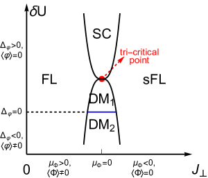
Figure 4: A schematic phase diagram at zero temperature with $J_{\perp}$ and $\delta U$ the tuning parameters, which effectively tune the mass of $\Phi$ ($\mu_{\Phi}$) and $\varphi$ ($\Delta_{\varphi}$). The tri-critical point is at $\mu_{\Phi}=0$ and $\Delta_{\varphi}=\Delta_{\varphi;c}=m_{f}^{2}/16$. When $\Delta_{\varphi}$ is smaller than $\Delta_{\varphi;c}$, there are two deconfined metal(DM) phases. In DM1 there are two deconfined gauge fields $a_{\mu}$ and $b_{\mu}$ while in DM2 $b_{\mu}$ is higgsed by $\langle\varphi\rangle\neq 0$.

The role of $\delta U$ is to add an energy penalty to the last two doublon states which violates the condition $n_{i;\psi_{t}}=n_{i;\psi_{b}}$: $H^{\prime}=\delta U\sum_{i}(n_{i;\psi_{t}}-n_{i;\psi_{b}})^{2}$. Now the previous local constraint $n_{i;\psi_{t}}=n_{i;\psi_{b}}$ is not exact anymore unless $\delta U=+\infty$. As the U(1) gauge field $b_{\mu}$ originates from this constraint, we expect that $b_{\mu}$ is alive at the large $\delta U$ regime, but should disappear in the small $\delta U$ regime. How do we capture this evolution? The best way is to introduce another slave rotor corresponding to

$$L_{i}=\frac{1}{2}\left(n_{i,\psi_{t}}-n_{i,\psi_{b}}\right)$$ (20)

for the doublon states. As illustrated in Fig. (1), the last two doublon states have $L=\pm 1$ while the first four doublon states have $L=0$. Now the $\delta U$ term enters as $H^{\prime}=4\delta U\sum_{i}L_{i}^{2}$. We also introduce the canonical conjugate $\phi_{i}$ which has the commutation relation $\left[\phi_{i},L_{j}\right]=i\delta_{ij}$ with $L_{j}$. Then in the $\phi$ representation we can write $L$ as $L_{i}=-i\frac{\partial}{\partial\phi_{i}}$. The physical electron operators now become

$$c_{i;t\sigma} =\sum_{\sigma^{\prime}}f^{\dagger}_{i;b\sigma^{\prime}}\psi_{i;b\sigma^{\prime}}\psi_{i;t\sigma}+f^{\dagger}_{i;t\bar{\sigma}}\psi_{i;t\bar{\sigma}}\psi_{i;t\sigma}\varphi_{i},$$ (21)

$$c_{i;b\sigma} =\sum_{\sigma^{\prime}}f^{\dagger}_{i;t\sigma^{\prime}}\psi_{i;t\sigma^{\prime}}\psi_{i;b\sigma}+f^{\dagger}_{i;b\bar{\sigma}}\psi_{i;b\bar{\sigma}}\psi_{i;b\sigma}\varphi^{\dagger}_{i},$$

where $\varphi_{i}=\exp\left(-i\phi_{i}\right)$ is the slave rotor which decreases $L$ by $1$. Under the internal U(1) gauge transformation associated with $a_{\mu}$, $\varphi$ doesn’t change. Under the internal gauge transformation associated $b_{\mu}$, $f_{i}\rightarrow f_{i}$, $\psi_{i;t}\rightarrow\psi_{i;t}e^{i\theta_{b}(i)}$, $\psi_{i;b}\rightarrow\psi_{i;b}e^{-i\theta_{b}(i)}$, $\varphi_{i}\rightarrow\varphi_{i}e^{-2i\theta_{b}(i)}$. So $\varphi$ couples to $-2b_{\mu}$, which can also be seen from the fact that the time component of $b_{\mu}$ enforces the constraint $n_{i;\psi_{t}}-n_{i,\psi_{b}}-2L_{i}=0$. Thus $\varphi$ becomes a higgs boson which controls the dynamics of the internal gauge field $b_{\mu}$. For the global $U(1)$ symmetry, $\varphi$ only change under the gauge transformation associated with $B_{\mu}$, in which $\psi\rightarrow\psi$, $f_{i;t}\rightarrow f_{i;t}e^{i\theta_{d}(i)}$, $f_{i;b}\rightarrow f_{i;b}e^{-i\theta_{d}(i)}$, $\varphi_{i}\rightarrow\varphi_{i}e^{2i\theta_{d}(i)}$. Thereby $\varphi$ couples to $-2b_{\mu}+2B_{\mu}$.

At small $\delta U$, there is no penalty for finite $|L_{i}|$. So we expect $\varphi$ to condense like the superfluid phase of a boson. On the other hand, at large $\delta U$, we should have fixed $L_{i}=0$, so $\varphi$ should be gapped, like the Mott insulator phase of a boson. Then $\delta U$ tunes a superfluid to Mott insulator transition of this extra slave rotor $\varphi$.

Our tri-critical theory consists of the critical theory Eq. 9 tuned by $J_{\perp}$ together with the superfluid to Mott transition of $\varphi$:

$$\mathcal{L}_{\mathrm{tc}} =\mathcal{L}_{\mathrm{c}}+\left|\left(\partial_{\mu}-i\left(-2b_{\mu}+2B_{\mu}\right)\right)\varphi\right|^{2}$$ (22)

$$+\Delta_{\varphi}\left|\varphi\right|^{2}+\lambda_{3}\left|\varphi\right|^{4}.$$

There is no first order time derivative term on $\varphi$ because under the mirror reflection symmetry which exchange two layers, $\varphi\leftrightarrow\varphi^{\dagger}$. So the action for $\varphi$ is relativistic, similar to the interaction tuned superfluid to Mott transition of bosons.

In Fig. 4 we show the schematic zero temperature phase diagram with two tuning parameters: $J_{\perp}$ which tunes the mass of $\Phi_{a}$ and $\delta U$ which tunes $\Delta_{\varphi}$, the gap of $\varphi$. Note that since $\varphi$ couples to $2b$, it contributes to the action of $b_{\mu}$ and modifies $e_{b,0}^{2}$ even when $\varphi$ is gapped. In Appendix. C we show that when $\Delta_{\varphi}>0$,

$$\frac{1}{e_{a,0}^{2}} =\frac{1}{6\pi m_{\psi}}+\frac{2}{3\pi m_{f}},$$ (23)

$$\frac{1}{e_{b,0}^{2}} =\frac{1}{6\pi m_{\psi}}+\frac{1}{6\pi\sqrt{\Delta_{\varphi}}}.$$

At a large $\delta U$, the mass $\Delta_{\varphi}$ is large, so we still have $e_{a,0}^{2}<e_{b,0}^{2}$ and pairing instability at $\mu_{\Phi}=0$ as discussed in the previous section. If we decrease $\delta U$ until the gap of $\varphi$ reaches the critical value $\Delta_{\varphi c}=m_{f}^{2}/16$. Now we have $e_{a,0}^{2}=e_{b,0}^{2}$, which means the repulsive and attractive interactions mediated by gauge fields are balanced at $\mu_{\Phi}=0$. In this case the superconducting region shrinks completely and FL transits to sFL directly when increasing $J_{\perp}$. This is the tri-critical point illustrated in our phase diagram. At this fine tuned value of $\delta U$, the DFFT fixed point can survive down to zero temperature.

As we further decrease $\delta U$ to get a smaller but still positive $\Delta_{\varphi}$, we have $e_{a,0}^{2}>e_{b,0}^{2}$. Now when $\mu_{\Phi}<0$, the $\psi$ Fermi surface is still stable to pairing and we have an intermediate phase with $f,\psi$ Fermi surfaces coupled to deconfined $a_{\mu}$ and $b_{\mu}$. This is roughly a stable phase similar to the DQCP and we call it deconfined metal (DM₁). Note that in DM₁ $f$ couples to $2a_{\mu}$ and $\psi$ couples to $a_{\mu}\pm b_{\mu}$ as in the DFFT critical regime. Lastly, if we decrease $\delta U$ until $\Delta_{\varphi}<0$, we will have $\langle\varphi\rangle\neq 0$ and $b_{\mu}$ is higgsed completely ( $b_{\mu}=B_{\mu}$ ). Then we have a different intermediate deconfined metal (DM₂) phase where $f$ couples to $2a_{\mu}$ and $\psi$ couples to $a_{\mu}$. The property of the DM phases should be similar to the critical regime of the DFFT discussed in the last section.

V Numerical result of the $4+4$-states model in one dimension: evidence of intermediate Luther-Emery liquid

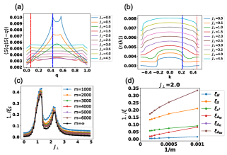
Figure 5: (a) the spin-spin correlation $\langle S(\bf{q})S(-{\bf q})\rangle$ for different $J_{\perp}$ , here $\vec{S}=\vec{S}_{t}+\vec{S}_{b}$ is the total spin. The red and blue line indicate the momentum $q=\frac{x}{2}$ and $q=\frac{1-x}{2}$ in units of $2\pi$, respectively. (b) $n({\bf k})=c_{t}^{\dagger}({\bf k})c_{t}({\bf k})$

. The red and blue line indicate the momentum $k=\frac{1}{2}-\frac{x}{4}$ and $k=\frac{1-x}{4}$ in units of $2\pi$, respectively. (c) (d) the spin correlation length vs $J_{\perp}$ and correlation length of different operators for $J_{\perp}=2$. In (c), the black line corresponds to $m=\infty$. The correlation length of $m=\infty$ is fitted from the relation $\frac{1}{\xi}=\frac{a}{m^{2}}+\frac{b}{m}+c$. In (d), we get the correlation length from the transfer matrix method. We can adjust three quantum numbers $N_{t}$, $N_{b}$, $S_{z}$ to access different operators. Here $N_{t},N_{b}$ are total electron numbers in the top and bottom layers and $S_{z}$ is the z component of the total spin. The correlation length of operators $N$, $S$, $c_{t\uparrow}^{\dagger}$, $\Delta_{tb}$, $\Delta_{tt}$, $\Delta_{bb}$, correspond to the largest eigenvalue of the transfer matrix in the charge sectors $(\delta N_{t},\delta N_{b},\delta S_{z})$=, $(0,0,0)$, $(0,0,1)$, $(1,0,\frac{1}{2})$, $(1,1,0)$, $(2,0,0)$, $(0,2,0)$. One can see that the dominant correlation lengths are from the density operator $N$ and the inter-layer pairing $\Delta_{tb}$.

We perform a infinite density matrix renormalization group (iDMRG)[40, 41] simulation of the $4+4$-states model. Without loss of generality, in our DMRG simulation, besides the terms in Eq. 4, we add the $SU(4)$ spin-spin interaction,

$$H^{\prime}=\frac{J}{2}\sum_{\langle ij\rangle}\sum_{ab}S^{ab}(i)S^{ba}(j),$$ (24)

where $S^{ab}$ is the $su(4)$ generator in the basis of $4+4$ states as defined in Appendix. D, and $a(b)$ is the combined indices of spin and layer. In our numerical simulation, we set the parameters $t=1$, $J=0.5$, and $L_{x}=22$, the doping level is $x=3/22$, and we increase the inter-layer spin interaction $J_{\perp}$ from $0$ to $6$. The bond dimension in our calculation is up to $m=6000$ and the truncation error is up to order $10^{-6}$.

In Fig. 5(a) and (b), we show the spin-spin correlation $\langle S({\bf q})S(-{\bf q})\rangle$ and the charge density $n({\bf k})$ in momentum space , as we increase the inter-layer spin interaction the Fermi surface size changes from $2k_{F}=\frac{1-x}{2}$ at small $J_{\perp}$ to $2k_{F}=\frac{x}{2}$ at large $J_{\perp}$, confirming the evolution from large Fermi surface at small $J_{\perp}$ to small Fermi surface at large $J_{\perp}$. We dub the two phases as Luttinger liquid (LL) and second Luttinger liquid (sLL), as analog of the FL and sFL phases we discussed in two dimension. In the appendix, we fit the central charge for different $J_{\perp}$, and we find the central charge in the LL and sLL is $c\approx 4$, while there is a intermediate regime with $c\approx 1$. In Fig. 5(c) and (d), we show inverse of the correlation lengths from different symmetry sectors as is obtained from the transfer matrix technique. In Fig. 5(c), the spin correlation length in the sLL and LL is divergent in the $m=\infty$ limit, while in the intermediate phase the spin correlation length is finite. We expect that the spin gap $\Delta_{s}\sim\xi_{S}^{-1}$, so there should be a dome of spin gap in the intermediate regime. In Fig. 5(d), we focus on $J_{\perp}=2$, the spin operator and the single electron operator are gapped with finite correlation length, while the density operator has an infinite correlation length at the infinite bond dimension limit $m\rightarrow\infty$. Meanwhile the correlation length of the inter-layer pairing, $\xi_{\Delta_{tb}}$ also diverges, consistent with the Luther-Emery liquid phase[42]. We also define an inter-layer Cooper pair $\Delta_{ll^{\prime}}(x)=\epsilon_{\sigma\sigma^{\prime}}c_{l}(x)c_{l^{\prime}}(x+1)$, where $l(l^{\prime})=t,b$ is the layer index. In Appendix. D, we show that the inter-layer pair-pair correlation function $\langle\Delta_{tb}^{\dagger}(x)\Delta_{tb}(0)\rangle$ shows a power law scaling with exponent around $3.8$, as expected in the Luther-Emery liquid[42]. The large exponent is presumably due to the small Luttinger parameter in our model because of the infinite on-site inter-layer repulsion.

Overall, our numerical results in one dimension is qualitative similar to the schematic phase diagram in Fig.3 at zero temperature for two dimension. We can clearly identify the analog of the FL and sFL phases in the two limit and an intermediate spin gapped Luther-Emery liquid phase analogous to the superconductor phase in higher dimension. Though the pairing correlation has a large power law exponent, this is likely special to one dimension. In higher dimension we expect long range ordered inter-layer pairing in the intermediate regime. Note that the existence of pairing is actually remarkable given that we have an infinite on-site interlayer repulsive interaction. This really indicates a new pairing mechanism associated with the critical region of a small to large Fermi surface transition.

VI conclusion

In summary, we propose a deconfined quantum critical point (DQCP) between two symmetric Fermi liquids in a bilayer model tuned by inter-layer spin coupling $J_{\perp}$, with a Fermi surface volume jump of $1/2$ Brillouin zone across the transition. Though the two sides are just conventional Fermi liquids, the critical regime is dominated by fractionalized fermions coupled to two emergent U(1) gauge fields, with the electron operator as a three-particle bound state. The critical point has an instability towards an intermediate superconductor dome with inter-layer pairing. We also show that tuning another parameter can suppress the pairing instability and lead to a deconfind tri-critical point. Our phase diagram shows certain similarity to the experimental phase diagram of the hole doped cuprates, with a small to large Fermi surface transition and an associated superconductor dome. But our setup is much cleaner due to the absence of the complexity from various symmetry breaking orders. We hope future investigation of this Fermi liquid to Fermi liquid transition can provide more insights on the general theory of the strange metal and its superconducting instability.

VII Acknowledgement

This work was supported by the National Science Foundation under Grant No. DMR-2237031.

Appendix A Mean field decomposition

In this section we show the mean-field Hamiltonian of Eq. (4). Plug the electron operators of parton form Eq. (7) into Eq. (4), we have

$$H =-t\sum_{\langle ij\rangle}\sum_{\sigma,\sigma_{1},\sigma_{2}}\left(\psi^{\dagger}_{i;t\sigma}\psi^{\dagger}_{i;b\sigma_{1}}f_{i;b\sigma_{1}}f^{\dagger}_{j;b\sigma_{2}}\psi_{j;b\sigma_{2}}\psi_{j;t\sigma}\right.$$ (25)

$$+\left.\psi^{\dagger}_{i;b\sigma}\psi^{\dagger}_{i;t\sigma_{1}}f_{i;t\sigma_{1}}f^{\dagger}_{j;t\sigma_{2}}\psi_{j;t\sigma_{2}}\psi_{j;b\sigma}\right)$$

$$+\frac{J_{\perp}}{4}\sum_{i}\left[\psi^{\dagger}_{i;t\sigma}\vec{\sigma}_{\sigma\sigma^{\prime}}\psi_{i;t\sigma^{\prime}}\right]\left[\psi^{\dagger}_{i;b\sigma}\vec{\sigma}_{\sigma\sigma^{\prime}}\psi_{i;b\sigma^{\prime}}\right].$$

We can define the following parameters,

$$\chi_{f;ij}= \sum_{\sigma}\langle f^{\dagger}_{i;t\sigma}f_{j;t\sigma}\rangle=\sum_{\sigma}\langle f^{\dagger}_{i;b\sigma}f_{j;b\sigma}\rangle,$$ (26)

$$\chi_{\psi;ij}= \sum_{\sigma}\langle\psi_{i;t\sigma}^{\dagger}\psi_{j;t\sigma}\rangle=\sum_{\sigma}\langle\psi_{i;b\sigma}^{\dagger}\psi_{j;b\sigma}\rangle,$$ (27)

$$\chi_{f\psi;i}= \sum_{\sigma}\langle f_{i;t\sigma}^{\dagger}\psi_{i;t\sigma}\rangle=\sum_{\sigma}\langle f_{i;b\sigma}^{\dagger}\psi_{i;b\sigma}\rangle,$$ (28)

$$\tilde{\Delta}_{i}= \sum_{\sigma\sigma^{\prime}}\epsilon_{\sigma\sigma^{\prime}}\langle\psi_{i;t\sigma}\psi_{i;b\sigma^{\prime}}\rangle=2\langle\psi_{i;t\uparrow}\psi_{b;\downarrow}\rangle=-2\langle\psi_{i;t\downarrow}\psi_{b;\uparrow}\rangle$$ (29)

here for simplicity, we consider all the parameters are in the trivial representation of the lattice symmetry, i.e., $\chi_{ij}=\chi$. In terms of these mean-field parameters, we can use the Wick theorem to obtain the following mean-field Hamiltonian:

$$H_{\mathrm{MF}}= \sum_{\langle ij\rangle}\left(t^{f}f^{\dagger}_{i;a\sigma}f_{j;a\sigma}+\mathrm{h.c.}\right)+\sum_{\langle ij\rangle}\left(-t^{\psi}\psi_{i;l\sigma}^{\dagger}\psi_{j;l\sigma}+\mathrm{h.c.}\right)$$ (30)

$$+ \sum_{i}\left(-\Phi_{a}f_{i;a\sigma}^{\dagger}\psi_{i;a\sigma}+\mathrm{h.c.}\right)+\sum_{i}\left(-\Delta\epsilon_{\sigma\sigma^{\prime}}\psi_{i;t\sigma}\psi_{i;b\sigma^{\prime}}+\mathrm{h.c.}\right)$$

$$- \sum_{i}\left(\mu_{f_{t}}(n_{i;f_{t}}-x)+\mu_{f_{b}}(n_{i;f_{b}}-x)+\mu_{\psi_{t}}(n_{\psi_{t}}-(1-2x))+\mu_{\psi_{b}}(n_{\psi_{b}}-(1-2x))\right),$$

The chemical potentials $\mu_{f}$ and $\mu_{\psi}$ are introduced to conserve the particle number. The self consistent equations are:

$$t^{f} =t\left(\frac{1}{2}\chi_{\psi}^{2}+\frac{1}{4}\tilde{\Delta}^{2}\right),$$ (31)

$$t^{\psi} =t\left(\chi_{f\psi}^{2}-\chi_{f}\chi_{\psi}\right),$$

$$\Phi_{a} =t\chi_{\psi}\chi_{f\psi},$$

$$\Delta =\left(2t\chi_{f}-\frac{3}{8}J_{\perp}\right)\tilde{\Delta}.$$

Appendix B Critical theory at large $\delta U$

In this section we perform a renormalization group analysis to the critical theory Eq. (9), which corresponds to large $\delta U$ case. We can tune $J_{\perp}$ (the mass $\mu_{\Phi}$) to reach the QCP at $\mu_{\Phi}=0$. We analyze the stability of this QCP while setting the external U(1) gauge fields $A=B=0$.

B.1 Self-Energy of the photon

We basically follow the calculation in [32]. After a renormalization of the gauge field Lagrangian from polarization corrections from the fermion $f$, $\Psi$ and, we obtain:

$$\mathcal{L}_{a,b}=\frac{1}{2}\left(\frac{1}{e_{a,0}^{2}}\left|\mathbf{q}\right|^{2}+\kappa_{a}\frac{|\omega|}{|\mathbf{q}|}\right)\left|a(\omega,\mathbf{q})\right|^{2}+\frac{1}{2}\left(\frac{1}{e_{b,0}^{2}}\left|\mathbf{q}\right|^{2}+\kappa_{b}\frac{|\omega|}{|\mathbf{q}|}\right)\left|b(\omega,\mathbf{q})\right|^{2},$$ (32)

where we use the Coulomb gauge so there is only one transverse component of each gauge field. The first term comes from the bubble diagrams of $f$ and $\psi$, while the second term only comes from $\psi$. Both terms include a Landau diamagnetic $\mathbf{q}^{2}$ term and a Landau damping $|\omega|/|\mathbf{q}|$ term. Note that the boson $\Phi_{a}$ does not contribute to $\mathcal{L}_{a,b}$ since its time derivative is of first order. The coupling constants $e^{2}$ and the Landau damping coefficients $\kappa$ are

$$\frac{1}{e_{a,0}^{2}} =\frac{1}{6\pi m_{\psi}}+\frac{2}{3\pi m_{f}},\quad\kappa_{a}=\frac{2m_{\psi}v_{F,\psi}}{\pi}+\frac{8m_{f}v_{F,f}}{\pi},$$ (33)

$$\frac{1}{e_{b,0}^{2}} =\frac{1}{6\pi m_{\psi}},\quad\quad\quad~{}~{}~{}\quad\kappa_{b}=\frac{2m_{\psi}v_{F,\psi}}{\pi}.$$

B.2 RG flow

We consider the coupling between fermions $f$, $\psi$ and gauge fields $a$,$b$. We use the $\epsilon$-expansion[36] to derive the RG equations. We consider the action

$$S=S_{a,b}+S_{f}+S_{\psi}$$ (34)

with

$$S_{a,b} =\frac{1}{2}\int\frac{d\omega d^{2}q}{(2\pi)^{3}}\left[\left(\frac{1}{e_{a}^{2}}|q_{y}|^{1+\epsilon}+\kappa_{a}\frac{|\omega|}{|q_{y}|}\right)\left|a(\omega,\mathbf{q})\right|^{2}+\left(\frac{1}{e_{b}^{2}}|q_{y}|^{1+\epsilon}+\kappa_{b}\frac{|\omega|}{|q_{y}|}\right)\left|b(\omega,\mathbf{q})\right|^{2}\right],$$ (35)

$$S_{f} =\int\frac{d\omega d^{2}k}{(2\pi)^{3}}\sum_{a=t,b}\bar{f}_{a;\sigma}\left(i\omega-v_{F,f}k_{x}-\frac{1}{2m_{f}}k_{y}^{2}\right)f_{a;\sigma}$$

$$+v_{F,f}\int\frac{d^{3}q}{(2\pi)^{3}}\int\frac{d\omega d^{2}k}{(2\pi)^{3}}\sum_{a=t,b}\bar{f}_{a;\sigma}(k+q)\cdot 2a(q)f_{a;\sigma}(k),$$

$$S_{\psi} =\int\frac{d\omega d^{2}k}{(2\pi)^{3}}\sum_{a=t,b}\bar{\psi}_{a;\sigma}\left(i\omega-v_{F,\psi}k_{x}-\frac{1}{2m_{\psi}}k_{y}^{2}\right)\psi_{a;\sigma}$$

$$+v_{F,\psi}\int\frac{d^{3}q}{(2\pi)^{3}}\int\frac{d\omega d^{2}k}{(2\pi)^{3}}\bar{\psi}_{t;\sigma}(k+q)\left(a(q)+b(q)\right)\psi_{t;\sigma}(k)$$

$$+v_{F,\psi}\int\frac{d^{3}q}{(2\pi)^{3}}\int\frac{d\omega d^{2}k}{(2\pi)^{3}}\bar{\psi}_{b;\sigma}(k+q)\left(a(q)-b(q)\right)\psi_{b;\sigma}(k).$$

We have scaling $[k_{x}]=1$, $[\omega]=1$, $[k_{y}]=\frac{1}{2}$, $[f]=[\psi]=-\frac{7}{4}$, $[a]=[b]=-\frac{3}{2}$, $[e_{a}^{2}]=[e_{b}^{2}]=\frac{\epsilon}{2}$, $[m_{f/\psi}]=[v_{F,f/\psi}]=0$. We define the new coupling constants $\alpha_{a,f}=\frac{e_{a}^{2}v_{F,f}}{4\pi^{2}}$, $\alpha_{b,f}=\frac{e_{b}^{2}v_{F,f}}{4\pi^{2}}$, $\alpha_{a,\psi}=\frac{e_{a}^{2}v_{F,\psi}}{4\pi^{2}}$ and $\alpha_{b,\psi}=\frac{e_{b}^{2}v_{F,\psi}}{4\pi^{2}}$. The naive scaling gives $[\alpha_{a}]=[\alpha_{b}]=\frac{\epsilon}{2}$.

To do the renormalization group analysis using $\epsilon$-expansion, we redefine the fields as follows:

$$f^{0} =Z_{f}^{1/2}f,$$ (36)

$$\psi^{0} =Z_{\psi}^{1/2}\psi,$$

$$v_{F,f}^{0} =Z_{v_{F,f}}v_{F,f},$$

$$v_{F,\psi}^{0} =Z_{v_{F,\psi}}v_{F,\psi},$$

$$e_{a}^{0} =\mu^{\frac{\epsilon}{4}}Z_{e_{a}}e_{a},$$

$$e_{b}^{0} =\mu^{\frac{\epsilon}{4}}Z_{e_{b}}e_{b},$$

$$a^{0} =Z_{a}a,$$

$$b^{0} =Z_{b}b,$$

and then we can rewrite the original action as

$$S =\frac{1}{2}\int\frac{d\omega d^{2}q}{(2\pi)^{3}}\left[\left(\frac{Z_{a}^{2}}{\mu^{\frac{\epsilon}{2}}Z_{e_{a}}^{2}e_{a}^{2}}|q_{y}|^{1+\epsilon}+Z_{a}^{2}\kappa_{a}\frac{|\omega|}{|q_{y}|}\right)|a(\omega,\mathbf{q})|^{2}\right]$$ (37)

$$+\frac{1}{2}\int\frac{d\omega d^{2}q}{(2\pi)^{3}}\left[\left(\frac{Z_{b}^{2}}{\mu^{\frac{\epsilon}{2}}Z_{e_{b}}^{2}e_{b}^{2}}|q_{y}|^{1+\epsilon}+Z_{b}^{2}\kappa_{b}\frac{|\omega|}{|q_{y}|}\right)|b(\omega,\mathbf{q})|^{2}\right]$$

$$+\int\frac{d\omega d^{2}k}{(2\pi)^{3}}\sum_{a=t,b}\bar{f}_{a;\sigma}\left(iZ_{f}\omega-Z_{f}Z_{v_{F,f}}v_{F,f}k_{x}-Z_{f}\frac{1}{2m_{f}}k_{y}^{2}\right)f_{a;\sigma}$$

$$+Z_{f}Z_{v_{F,f}}v_{F,f}\int\frac{d^{3}q}{(2\pi)^{3}}\int\frac{d\omega d^{2}k}{(2\pi)^{3}}\sum_{a=t,b}\bar{f}_{a;\sigma}(k+q)\cdot 2Z_{a}a(q)f_{a;\sigma}(k)$$

$$+\int\frac{d\omega d^{2}k}{(2\pi)^{3}}\sum_{a=t,b}\bar{\psi}_{a;\sigma}\left(iZ_{\psi}\omega-Z_{\psi}Z_{v_{F,\psi}}v_{F,\psi}k_{x}-Z_{\psi}\frac{1}{2m_{\psi}}k_{y}^{2}\right)\psi_{a;\sigma}$$

$$+Z_{\psi}Z_{v_{F,\psi}}v_{F,\psi}\int\frac{d^{3}q}{(2\pi)^{3}}\int\frac{d\omega d^{2}k}{(2\pi)^{3}}\bar{\psi}_{t;\sigma}(k+q)\left(Z_{a}a(q)+Z_{b}b(q)\right)\psi_{t;\sigma}(k)$$

$$+Z_{\psi}Z_{v_{F,\psi}}v_{F,\psi}\int\frac{d^{3}q}{(2\pi)^{3}}\int\frac{d\omega d^{2}k}{(2\pi)^{3}}\bar{\psi}_{b;\sigma}(k+q)\left(Z_{a}a(q)-Z_{b}b(q)\right)\psi_{b;\sigma}(k).$$

From the Ward identity, we expect $Z_{a}=Z_{b}=1$. Hence the fermion-gauge field vertex correction should be purely from $Z_{f}Z_{v_{F,f}}$ and $Z_{\psi}Z_{v_{F,\psi}}$. It can be shown that they both equal to 1, implying that there is no vertex correction. When $\epsilon<1$, we expect $Z_{e_{a}}=Z_{e_{b}}=1$ because the non-analytic form $|q_{y}|^{1+\epsilon}$ cannot be renormalized. Therefore the only important renormalization is from $Z_{f}=Z_{v_{F,f}}^{-1}$ and $Z_{\psi}=Z_{v_{F,\psi}}^{-1}$.

The self-energy of $f$ at one-loop order is

$$\Sigma_{f}(i\omega) =\frac{4e_{a}^{2}v_{F,f}^{2}}{(2\pi)^{3}}\int dq_{0}d^{2}q\frac{1}{|q_{y}|^{1+\epsilon}+\kappa_{a}e_{a}^{2}\frac{|q_{0}|}{|q_{y}|}}\frac{1}{i\omega+iq_{0}-v_{F,f}(k_{x}+q_{x})-\frac{1}{2m_{f}}(k_{y}+q_{y})^{2}}$$ (38)

$$=2\alpha_{a,f}\int dq_{0}dq_{y}\frac{i\textrm{sign}(\omega+q_{0})}{|q_{y}|^{1+\epsilon}+\kappa_{a}e_{a}^{2}\frac{|q_{0}|}{|q_{y}|}}$$

$$=4\alpha_{a,f}\frac{1}{\epsilon}\int dq_{0}i\textrm{sign}(\omega+q_{0})+...$$

$$=8\alpha_{a,f}i\omega\frac{1}{\epsilon}.$$

In the above we only keep the divergent part $\mathcal{O}(1/\epsilon)$. To cancel the divergence, we need

$$Z_{f}=Z_{v_{F,f}}^{-1}=1-8\alpha_{a,f}\frac{1}{\epsilon}+\mathcal{O}(\frac{1}{\epsilon^{2}}).$$ (39)

The self-energy of $\psi$ at one-loop order is

$$\Sigma_{\psi}(i\omega) =\frac{e_{a}^{2}v_{F,\psi}^{2}}{(2\pi)^{3}}\int dq_{0}d^{2}q\frac{1}{|q_{y}|^{1+\epsilon}+\kappa_{a}e_{a}^{2}\frac{|q_{0}|}{|q_{y}|}}\frac{1}{i\omega+iq_{0}-v_{F,\psi}(k_{x}+q_{x})-\frac{1}{2m_{\psi}}(k_{y}+q_{y})^{2}}$$ (40)

$$+\frac{e_{b}^{2}v_{F,\psi}^{2}}{(2\pi)^{3}}\int dq_{0}d^{2}q\frac{1}{|q_{y}|^{1+\epsilon}+\kappa_{b}e_{b}^{2}\frac{|q_{0}|}{|q_{y}|}}\frac{1}{i\omega+iq_{0}-v_{F,\psi}(k_{x}+q_{x})-\frac{1}{2m_{\psi}}(k_{y}+q_{y})^{2}}$$

$$=\frac{\alpha_{a,\psi}}{2}\int dq_{0}d^{2}q\frac{i\textrm{sign}(\omega+q_{0})}{|q_{y}|^{1+\epsilon}+\kappa_{a}e_{a}^{2}\frac{|q_{0}|}{|q_{y}|}}+\frac{\alpha_{b,\psi}}{2}\int dq_{0}d^{2}q\frac{i\textrm{sign}(\omega+q_{0})}{|q_{y}|^{1+\epsilon}+\kappa_{b}e_{b}^{2}\frac{|q_{0}|}{|q_{y}|}}$$

$$=\left(\alpha_{a,\psi}+\alpha_{b,\psi}\right)\frac{1}{\epsilon}\int dq_{0}i\textrm{sign}(\omega+q_{0})+...$$

$$=2\left(\alpha_{a,\psi}+\alpha_{b,\psi}\right)i\omega\frac{1}{\epsilon}$$

therefore

$$Z_{\psi}=Z_{v_{F,\psi}}^{-1}=1-2\left(\alpha_{a,\psi}+\alpha_{b,\psi}\right)\frac{1}{\epsilon}+\mathcal{O}(\frac{1}{\epsilon^{2}}).$$ (41)

Next, we show explicitly that the vertex correction vanishes. For simplicity we use $a\bar{f}f$ as an illustration. We have

$$\delta\Gamma^{c}(p_{0},p_{x},p_{y}) =\int\frac{d^{3}q}{2\pi}\frac{1}{iq_{0}-v_{F,f}q_{x}-\frac{1}{2K_{f}}q_{y}^{2}}\frac{1}{iq_{0}+ip_{0}-v_{F,f}(q_{x}+p_{x})-\frac{1}{2K_{f}}(q_{y}+p_{y})^{2}}\frac{4\alpha_{a,f}v_{F,f}}{|q_{y}|^{1+\epsilon}+\kappa_{a}e_{a}^{2}\frac{|q_{0}|}{|q_{y}|}}$$ (42)

$$=i\textrm{sign}(p_{0})\int dq_{y}\int_{0}^{|p_{0}|}dq_{0}\frac{4\alpha_{a,f}}{|q_{y}|^{1+\epsilon}+\kappa_{a}e_{a}^{2}\frac{|q_{0}|}{|q_{y}|}}\frac{1}{ip_{0}-v_{F,f}p_{x}-\frac{1}{K_{f}}p_{y}q_{y}-\frac{1}{2K_{f}}p_{y}^{2}},$$

where $(p_{0},p_{x},p_{y})$ is the external momentum of $a$ photon at the vertex. We assume one of the external $f$ fermion at the vertex has zero momentum. In the first step we integrate over $q_{x}$ and get a factor $\textrm{sign}(p_{0}+q_{0})-\textrm{sign}(q_{0})$, which equals to 2 for $q_{0}\in[-p_{0},0]$ and zero otherwise. We can see that $\delta\Gamma^{c}(p_{0}=0,p_{x},p_{y})=0$ so there is no vertex correction. The same conclusion holds for every fermion-gauge field vertex.

Finally, we can get the beta functions $\beta(\alpha)=-d\alpha/d\log\mu$ (note that this is the negative of the usual definition) from the relations

$$\alpha_{a,f}^{0} =\mu^{\frac{\epsilon}{2}}Z_{e_{a}}^{2}Z_{v_{F,f}}\alpha_{a,f},$$ (43)

$$\alpha_{b,f}^{0} =\mu^{\frac{\epsilon}{2}}Z_{e_{b}}^{2}Z_{v_{F,f}}\alpha_{b,f},$$

$$\alpha_{a,\psi}^{0} =\mu^{\frac{\epsilon}{2}}Z_{e_{a}}^{2}Z_{v_{F,\psi}}\alpha_{a,\psi},$$

$$\alpha_{b,\psi}^{0} =\mu^{\frac{\epsilon}{2}}Z_{e_{b}}^{2}Z_{v_{F,\psi}}\alpha_{b,\psi}.$$

Using $d\log\alpha^{0}/d\log\mu=0$ and $Z_{e_{a}}=Z_{e_{b}}=1$, we have

$$0=-\frac{\epsilon}{2}-\frac{d\log\alpha}{d\log\mu}-\frac{d\log Z_{v_{F}}}{d\log\mu}=-\frac{\epsilon}{2}-\frac{d\log\alpha}{d\log\mu}+\frac{d\log Z}{d\log\mu}$$ (44)

where in the second step we use the relation $Z_{f}Z_{v_{F,f}}=Z_{\psi}Z_{v_{F,\psi}}=1$. We have equations:

$$\left(1-\alpha_{a,f}\frac{\partial\log Z_{f}}{\partial\alpha_{a,f}}\right)\beta(\alpha_{a,f})=\frac{\epsilon}{2}\alpha_{a,f},$$ (45)

$$\beta(\alpha_{b,f})-\alpha_{b,f}\frac{\partial\log Z_{f}}{\partial\alpha_{a,f}}\beta(\alpha_{a,f})=\frac{\epsilon}{2}\alpha_{b,f},$$ (46)

$$\left(1-\alpha_{a,\psi}\frac{\partial\log Z_{\psi}}{\partial\alpha_{a,\psi}}\right)\beta(\alpha_{a,\psi})-\alpha_{a,\psi}\frac{\partial\log Z_{\psi}}{\partial\alpha_{b,\psi}}\beta(\alpha_{b,\psi})=\frac{\epsilon}{2}\alpha_{a,\psi},$$ (47)

$$-\alpha_{b,\psi}\frac{\partial\log Z_{\psi}}{\partial\alpha_{a,\psi}}\beta(\alpha_{a,\psi})+\left(1-\alpha_{b,\psi}\frac{\partial\log Z_{\psi}}{\partial\alpha_{b,\psi}}\right)\beta(\alpha_{b,\psi})=\frac{\epsilon}{2}\alpha_{b,\psi}.$$ (48)

Using

$$\log Z_{f} =-8\alpha_{a,f}\frac{1}{\epsilon}+\mathcal{O}(\frac{1}{\epsilon^{2}}),$$ (49)

$$\log Z_{\psi} =-2\left(\alpha_{a,\psi}+\alpha_{b,\psi}\right)\frac{1}{\epsilon}+\mathcal{O}(\frac{1}{\epsilon^{2}}),$$

and the fact that all $\mathcal{O}(1/\epsilon^{n})$ terms should vanish for the theory to be renormalizable, we obtain the beta functions:

$$\beta(\alpha_{a,f}) =\frac{\epsilon}{2}\alpha_{a,f}-4\alpha_{a,f}^{2}$$ (50)

$$\beta(\alpha_{b,f}) =\frac{\epsilon}{2}\alpha_{b,f}-4\alpha_{a,f}\alpha_{b,f}$$

$$\beta(\alpha_{a,\psi}) =\frac{\epsilon}{2}\alpha_{a,\psi}-\alpha_{a,\psi}\left(\alpha_{a,\psi}+\alpha_{b,\psi}\right)$$

$$\beta(\alpha_{b,\psi}) =\frac{\epsilon}{2}\alpha_{b,\psi}-\alpha_{b,\psi}\left(\alpha_{a,\psi}+\alpha_{b,\psi}\right)$$

We can see that there are fixed points satisfying $\alpha_{a,f}=\epsilon/8$ and $\alpha_{a,\psi}+\alpha_{b,\psi}=\epsilon/2$. We also find that the ratio $\alpha_{a,\psi}/\alpha_{b,\psi}$ doesn’t flow, which shows that $\alpha_{a,\psi}-\alpha_{b,\psi}$ doesn’t change sign.

B.3 Pairing instability

The leading contribution to the interaction in BCS channel for fermions is from exchange of one photon. Among all the fermion pairing terms, the following one is the most important:

$$S_{BCS}=\int\prod d^{2}k_{i}d\omega_{i}\bar{\psi}_{t}(k_{1})\bar{\psi}_{b}(-k_{1})\psi_{b}(-k_{2})\psi_{t}(k_{2})VF(k_{1}-k_{2}),$$ (51)

where $F(q=k_{1}-k_{2})$ arises from the propagator of photons. Note that $\psi_{t}$ couples to $a+b$ while $\psi_{b}$ couples to $a-b$, which means that $a$ mediates repulsive interaction between $\psi_{t}$ and $\psi_{b}$ while $b$ mediates attractive interaction. The final sign of the interaction between $\psi_{t}$ and $\psi_{b}$ depends on the competition between $a$ and $b$.

We define dimensionless BCS interaction constant

$$\tilde{V}_{m}=\frac{k_{F,\psi}}{2\pi v_{F,\psi}}V_{m},$$ (52)

where $m$ is the angular momentum for the corresponding pairing channel. By integrating out photon in the intermediate energy, we obtain

$$\delta\tilde{V}_{m} =\frac{k_{F,\psi}}{2\pi v_{F,\psi}}v_{F,\psi}^{2}\int\frac{d\theta}{2\pi}\left(\frac{e^{-im\theta}}{|k_{F,\psi}\theta|^{1+\epsilon}/e_{a}^{2}}-\frac{e^{-im\theta}}{|k_{F,\psi}\theta|^{1+\epsilon}/e_{b}^{2}}\right)$$ (53)

$$=\frac{v_{F,\psi}}{4\pi^{2}}2\int_{\Lambda_{y}e^{-\delta l/2}}^{\Lambda_{y}}dq_{y}\left(\frac{1}{|q_{y}|^{1+\epsilon}/e_{a}^{2}}-\frac{1}{|q_{y}|^{1+\epsilon}/e_{b}^{2}}\right)$$

$$=\left(\alpha_{a,\psi}-\alpha_{b,\psi}\right)\delta l.$$

The renormalization in Eq. (53) should be combined with the usual flow of the BCS interaction to obtain the RG equation:

$$\frac{d\tilde{V}}{dl}=\left(\alpha_{a,\psi}-\alpha_{b,\psi}\right)-\tilde{V}^{2}.$$ (54)

From Eq. (33) we have bare values $\alpha^{0}_{a,\psi}-\alpha^{0}_{b,\psi}<0$, then $\tilde{V}$ will flow to $-\infty$. Considering the case $\epsilon=0$, then from Eq. (50) we obtain

$$\alpha_{a,\psi}(l) =\frac{\alpha_{a,\psi}(0)}{1+\left(\alpha_{a,\psi}(0)+\alpha_{b,\psi}(0)\right)l},$$ (55)

$$\alpha_{b,\psi}(l) =\frac{\alpha_{b,\psi}(0)}{1+\left(\alpha_{a,\psi}(0)+\alpha_{b,\psi}(0)\right)l},$$

where we identify $-\log\mu$ as $l$. The decreasing of $\alpha$ is slow so we can approximately use the bare value when solving Eq. (54). We get

$$\tilde{V}(l)=\sqrt{\alpha_{b,\psi}^{0}-\alpha_{a,\psi}^{0}}\tan\left(-\sqrt{\alpha_{b,\psi}^{0}-\alpha_{a,\psi}^{0}}l+\tan^{-1}\frac{\tilde{V}(0)}{\sqrt{\alpha_{b,\psi}^{0}-\alpha_{a,\psi}^{0}}}\right).$$ (56)

We can see that $\tilde{V}(l)$ diverges at

$$l_{p}=\frac{1}{\sqrt{\alpha_{b,\psi}^{0}-\alpha_{a,\psi}^{0}}}\left(\frac{\pi}{2}+\tan^{-1}\frac{\tilde{V}(0)}{\sqrt{\alpha_{b,\psi}^{0}-\alpha_{a,\psi}^{0}}}\right),$$ (57)

which also gives a estimation of the superconducting gap $\Delta\sim\Lambda_{\omega}\exp(-l_{p})$. In the limit $\tilde{V}(0)\ll\sqrt{\alpha_{b,\psi}^{0}-\alpha_{a,\psi}^{0}}$ , we have $l_{p}\approx\pi/2\sqrt{\alpha_{b,\psi}^{0}-\alpha_{a,\psi}^{0}}$. In the limit $\tilde{V}(0)\gg\sqrt{\alpha_{b,\psi}^{0}-\alpha_{a,\psi}^{0}}$, we have $l_{p}\approx\pi/\sqrt{\alpha_{b,\psi}^{0}-\alpha_{a,\psi}^{0}}$. Here $\Lambda_{\omega}$ is the high energy cutoff of RG.

Appendix C Pairing instability in the tricritical theory

Now the photon self-energy is given by the polarization corrections from the fermion $f$, $\psi$ and boson $\varphi$. The contribution from $\varphi$ bubble is

$$\delta\Pi^{\mu\nu}(q) =4\int\frac{d^{3}l}{(2\pi)^{3}}\left[\frac{(2l+q)^{\mu}(2l+q)^{\nu}}{\left((l+q)^{2}+\Delta_{\varphi}\right)\left(l^{2}+\Delta_{\varphi}\right)}-\frac{2\delta^{\mu\nu}}{l^{2}+\Delta_{\varphi}}\right]$$ (58)

$$=\int_{-\frac{1}{2}}^{\frac{1}{2}}dy\frac{2y^{2}}{\pi\sqrt{\left(\frac{1}{4}-y^{2}\right)q^{2}+\Delta_{\varphi}}}\left(q^{2}\delta^{\mu\nu}-q^{\mu}q^{\nu}\right).$$

The factor 4 comes from the fact that $\varphi$ couples to $-2b_{\mu}$. The Feynman parametrization is used to get the second line. It has different behaviors for $\Delta_{\varphi}>0$ and $\Delta_{\varphi}=0$:

$$\Delta_{\varphi}=0:~{}~{}~{}\delta\Pi^{\mu\nu}=\frac{q^{2}\delta^{\mu\nu}-q^{\mu}q^{\nu}}{4\left|q\right|},$$ (59)

$$\Delta_{\varphi}>0:~{}~{}~{}\delta\Pi^{\mu\nu}=\frac{q^{2}\delta^{\mu\nu}-q^{\mu}q^{\nu}}{6\pi\sqrt{\Delta_{\varphi}}}+\mathcal{O}(q^{4}).$$

Combining all the polarization corrections from $f$, $\psi$ and $\varphi$, for $\Delta_{\varphi}>0$ and $\mu_{\Phi}=0$ we have

$$\mathcal{L}_{a,b}=\frac{1}{2}\left(\frac{1}{e_{a,0}^{2}}\left|\mathbf{q}\right|^{2}+\kappa_{a}\frac{\left|\omega\right|}{\left|\mathbf{q}\right|}\right)\left|a(\omega,\mathbf{q})\right|^{2}+\frac{1}{2}\left(\frac{1}{e_{a,0}^{2}}\left|\mathbf{q}\right|^{2}+\kappa_{a}\frac{\left|\omega\right|}{\left|\mathbf{q}\right|}\right)\left|b(\omega,\mathbf{q})\right|^{2},$$ (60)

where the coupling constants $e^{2}$ are

$$\frac{1}{e_{a,0}^{2}} =\frac{1}{6\pi m_{\psi}}+\frac{2}{3\pi m_{f}},$$ (61)

$$\frac{1}{e_{b,0}^{2}} =\frac{1}{6\pi m_{\psi}}+\frac{1}{6\pi\sqrt{\Delta_{\varphi}}}.$$

Note that all the RG analysis in Appendix. B is still valid when $\varphi$ is gapped. At $\Delta_{\varphi}=\Delta_{\varphi c}=\frac{1}{16}m_{f}^{2}$, we have $e_{b,0}^{2}=e_{a,0}^{2}$. The attractive and repulsive interactions mediated by gauge fields are balanced.

Appendix D Details of DMRG

In our DMRG simulation, we define all the operators in the $4+4$-states basis,

$$\ket{t\uparrow},\ket{t\downarrow},\ket{b\uparrow},\ket{b\downarrow},\ket{t\uparrow}\ket{b\uparrow},\ket{t\uparrow}\ket{b\downarrow},\ket{t\downarrow}\ket{b\uparrow},\ket{t\downarrow}\ket{b\downarrow}.$$ (62)

From Eq. 1, we can get the $SU(4)$ spin interaction $\frac{J}{2}c^{\dagger}_{a}(i)c_{b}(i)c_{b}^{\dagger}(j)c_{a}(j)=\frac{J}{2}S^{ab}(i)S^{ba}(j)$ from second order perturbation with $S^{ab}=c_{a}^{\dagger}c_{b}$, where $a(b)$ is the combined indices of spin and layer. In our numerical simulation we project the $su(4)$ operators $S^{ab}$ into the $4+4$-states Hilbert space.

D.1 More detailed results

In Fig. 6, we present more detailed DMRG results. Fig. 6(a) and (b) are the central charge for different $J_{\perp}$. We find in the LL and sLL phases where the central charge is $c\approx 4$ and the spin correlation length is very large, while in the intermediate phase, the central charge is $c\approx 1$. In Fig. 6(b), we use the formula $S=\frac{c}{6}\log\xi$ to fit the central charge, and in Fig. 6(c) shows the power law scaling of the inter-layer pair-pair correlation function of $J_{\perp}=2$. The intermediate phase is consistent with the Luther-Emery liquid[42]. The spin gapped Luther Emery liquid phase should be in the regime $J_{\perp}\in[J_{\perp}^{c1},J_{\perp}^{c2}]$. To further distinguish the phase boundary, we fit the central charge for small $J_{\perp}$ and large $J_{\perp}$ in Fig. 7 and Fig. 8. From the data, $J_{\perp}^{c1}$ should be around 0.4. It is not easy to fix the exact value of $J_{\perp}^{c2}$. The central charge is larger than $c=1$ when $J_{\perp}>2.5$, but is still smaller than $c=4$ within our bond dimension. In the main text we find that $\langle\vec{S}(q)\cdot\vec{S}(-q)\rangle$ already show peak at $q=\frac{x}{2}$ when $J_{\perp}\geq 3$, consistent with the sLL phase. This may suggest that $J_{\perp}^{c2}\approx 3$, but it is also tricky to decide whether there is a very small but finite spin gap. We leave to future work to decide whether the region with $J_{\perp}$ slightly larger than $3$ is in the sLL phase or actually has a small spin gap. But even if there is a finite spin gap, it only matters below a very small energy scale and hence is not that important in real experiments with a small temperature.

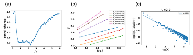
Figure 6: (a) central charge of different $J_{\perp}$. (b) the fitted central charge of different $J_{\perp}$. We use the relation $S=\frac{c}{6}\log\xi$ to fit the central charge, where $S$ is the entanglement entropy and $\xi$ is the correlation length. (c) the power law scaling of the pair-pair correlation function $\langle\Delta_{tb}^{\dagger}(x)\Delta_{tb}(0)\rangle$, where we use the formula $|\langle\Delta_{tb}^{\dagger}(x)\Delta_{tb}(0)\rangle|=\frac{A}{x^{\alpha}}$ to fit the numerical result.

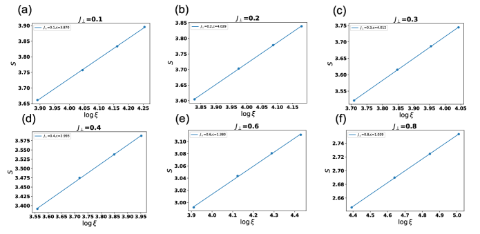
Figure 7: (a)-(f) the fitted central charge of $J_{\perp}=0,0.2,0.3,0.4,0.6,0.8$, respectively.

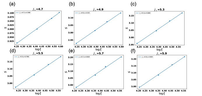
Figure 8: (a)-(f) the fitted central charge of $J_{\perp}=4.7,4.9,5.3,5.5,5.7,5.9$, respectively.

References

- Senthil et al. [2004a] T. Senthil, A. Vishwanath, L. Balents, S. Sachdev, and M. P. Fisher, Science 303, 1490 (2004a).
- Senthil [2023] T. Senthil, arXiv preprint arXiv:2306.12638 (2023).
- Wang and You [2022] J. Wang and Y.-Z. You, Symmetry 14, 1475 (2022).
- Tong [2022] D. Tong, Journal of High Energy Physics 2022, 1 (2022).
- You et al. [2018] Y.-Z. You, Y.-C. He, C. Xu, and A. Vishwanath, Physical Review X 8, 011026 (2018).
- Coleman et al. [2001] P. Coleman, C. Pépin, Q. Si, and R. Ramazashvili, Journal of Physics: Condensed Matter 13, R723 (2001).
- Gegenwart et al. [2008] P. Gegenwart, Q. Si, and F. Steglich, nature physics 4, 186 (2008).
- Si and Steglich [2010] Q. Si and F. Steglich, Science 329, 1161 (2010).
- Stewart [2001] G. Stewart, Reviews of modern Physics 73, 797 (2001).
- Coleman and Schofield [2005] P. Coleman and A. J. Schofield, Nature 433, 226 (2005).
- Löhneysen et al. [2007] H. v. Löhneysen, A. Rosch, M. Vojta, and P. Wölfle, Reviews of Modern Physics 79, 1015 (2007).
- Senthil et al. [2005] T. Senthil, S. Sachdev, and M. Vojta, Physica B: Condensed Matter 359, 9 (2005).
- Kirchner et al. [2020] S. Kirchner, S. Paschen, Q. Chen, S. Wirth, D. Feng, J. D. Thompson, and Q. Si, Reviews of Modern Physics 92, 011002 (2020).
- Lee et al. [2006] P. A. Lee, N. Nagaosa, and X.-G. Wen, Reviews of modern physics 78, 17 (2006).
- Sachdev [2003] S. Sachdev, Reviews of Modern Physics 75, 913 (2003).
- Phillips et al. [2022] P. W. Phillips, N. E. Hussey, and P. Abbamonte, Science 377, eabh4273 (2022).
- Proust and Taillefer [2019] C. Proust and L. Taillefer, Annual Review of Condensed Matter Physics 10, 409 (2019).
- Hertz [1976] J. A. Hertz, Physical Review B 14, 1165 (1976).
- Millis [1993] A. Millis, Physical Review B 48, 7183 (1993).
- Senthil et al. [2004b] T. Senthil, M. Vojta, and S. Sachdev, Physical Review B 69, 035111 (2004b).
- Senthil [2008] T. Senthil, Physical Review B 78, 045109 (2008).
- Zhang and Sachdev [2020a] Y.-H. Zhang and S. Sachdev, Physical Review B 102, 155124 (2020a).
- Oh and Zhang [2023] H. Oh and Y.-H. Zhang, arXiv preprint arXiv:2307.15706 (2023).
- Lu et al. [2023a] C. Lu, Z. Pan, F. Yang, and C. Wu, “Interlayer coupling driven high-temperature superconductivity in la3ni2o7 under pressure,” (2023a), arXiv:2307.14965 [cond-mat.supr-con] .
- Qu et al. [2023] X.-Z. Qu, D.-W. Qu, J. Chen, C. Wu, F. Yang, W. Li, and G. Su, arXiv preprint arXiv:2307.16873 (2023).
- Yang et al. [2023] H. Yang, H. Oh, and Y.-H. Zhang, “Strong pairing from small fermi surface beyond weak coupling: Application to la3ni2o7,” (2023), arXiv:2309.15095 [cond-mat.str-el] .
- Lange et al. [2023] H. Lange, L. Homeier, E. Demler, U. Schollwöck, A. Bohrdt, and F. Grusdt, arXiv e-prints , arXiv:2309.13040 (2023), arXiv:2309.13040 [cond-mat.str-el] .
- Oshikawa [2000] M. Oshikawa, Physical Review Letters 84, 3370 (2000).
- Note [1] By featureless we mean that the phase does not have fractionalization.
- Zhang and Mao [2020] Y.-H. Zhang and D. Mao, Physical Review B 101, 035122 (2020).
- Lu et al. [2023b] D.-C. Lu, M. Zeng, J. Wang, and Y.-Z. You, Physical Review B 107, 195133 (2023b).
- Zhang and Sachdev [2020b] Y.-H. Zhang and S. Sachdev, Physical Review Research 2, 023172 (2020b).
- Zou and Chowdhury [2020a] L. Zou and D. Chowdhury, Physical Review Research 2, 023344 (2020a).
- Zou and Chowdhury [2020b] L. Zou and D. Chowdhury, Physical Review Research 2, 032071 (2020b).
- Bohrdt et al. [2022] A. Bohrdt, L. Homeier, I. Bloch, E. Demler, and F. Grusdt, Nature Physics 18, 651 (2022).
- Metlitski et al. [2015] M. A. Metlitski, D. F. Mross, S. Sachdev, and T. Senthil, Phys. Rev. B 91, 115111 (2015).
- Polyakov [1987] A. M. Polyakov, Gauge fields and strings (Taylor & Francis, 1987).
- Lee [2018] S.-S. Lee, Annual Review of Condensed Matter Physics 9, 227 (2018).
- Else et al. [2021] D. V. Else, R. Thorngren, and T. Senthil, Physical Review X 11, 021005 (2021).
- White [1992] S. R. White, Phys. Rev. Lett. 69, 2863 (1992).
- McCulloch [2008] I. P. McCulloch, arXiv e-prints , arXiv:0804.2509 (2008), arXiv:0804.2509 [cond-mat.str-el] .
- Luther and Emery [1974] A. Luther and V. J. Emery, Phys. Rev. Lett. 33, 589 (1974).