CO emission survey of asymptotic giant branch stars with ultraviolet excesses

Abstract

Context. The transition from the spherically symmetric envelopes around asymptotic giant branch (AGB) stars to the asymmetric morphologies observed in planetary nebulae is still not well understood, and the shaping mechanisms are a subject of debate. Even though binarity is widely accepted as a promising option, it is limited by the complication of identifying binary AGB stars observationally. Recently, the presence of ultraviolet excesses in AGB stars has been suggested as a potential indicator of binarity.

Aims. Our main goals are to characterise the properties of the circumstellar envelopes (CSEs) around candidate AGB binary stars, specifically those selected based on their UV excess emission, and to compare these properties with those derived from previous CO-based studies of AGB stars.

Methods. We observed the ¹²CO ($J$=1–0) and ¹²CO ($J$=2–1)  millimetre-wavelength emission in a sample of 29 AGB binary candidates with the IRAM-30 m antenna. We measured the systemic velocities and the terminal expansion velocities from their line profiles. Population diagrams were used to interpret the results, enabling the estimation of excitation temperatures ($T_{\rm ex}$), mass-loss rates ($\dot{M}$), and the characteristic sizes of the envelope layers where the CO millimetre emission originates ($R_{\rm s}$). We explored different trends between the envelope parameters deduced, multiwavelength flux measurements, and other properties of our sample, and compared them with those previously derived from larger samples of AGB stars found in the literature.

Results. We detected ¹²CO emission in 15 sources, of which 5 are first detections. We found relatively low expansion velocities (3 km s^-1 $\lesssim$ $V_{\rm exp}$ $\lesssim$ 20 km s^-1) in our sample. We derived the average excitation temperature and column density of the CO-emitting layers, which we used to estimate self-consistently the average mass-loss rate ($10^{-8}$ $M_{\odot}$ yr^-1 $\lesssim$ $\dot{M}$ $\lesssim$ $10^{-5}$ $M_{\odot}$ yr^-1) and the CO photodissociation radius (5 $\times 10^{\rm 15}$ cm $\lesssim$ $R_{\rm CO}$ $\lesssim$ 2 $\times 10^{\rm 17}$ cm) of our targets. We find a correlation between CO intensity and IRAS 60$\mu$m  fluxes, revealing a CO-to-IRAS 60$\mu$m ratio lower than for AGB stars and closer to that found for pre-planetary nebulae (pPNe). An anti-correlation is observed between ¹²CO (and IRAS 60$\mu$m) and the near-ultraviolet (NUV), but no such correlation is observed with the far-ultraviolet (FUV). It is also worth noting that there is no correlation between bolometric luminosity and NUV or FUV.

Conclusions. For the first time we have studied the mass-loss properties of UV-excess AGB binary candidates and estimated their main CSE parameters. Our sample of uvAGB stars shows similarities with the broader category of AGB stars, except for a distinct CO-to-IRAS 60$\mu$m trend suggesting enhanced CO photodissociation. Our findings, based on single-dish low-$J$ CO line emission observations, support the dust-driven wind scenario and indicate that alternative mass-loss mechanisms are not necessary (in principle) to explain the $\sim$200-2000 yr old mass-loss ejecta in uvAGBs. The different relationships between ¹²CO and IRAS 60$\mu$m, with NUV and FUV are consistent with an intrinsic origin of NUV emission, but potential dominance of an extrinsic process (e.g. presence of a binary companion) in FUV emission.

1 Introduction

Most stars (i.e. with masses in the 1-8 $M_{\odot}$  range) evolve from the main sequence to the Asymptotic Giant Branch (AGB) phase and develop dusty winds producing spherically symmetric CSEs expanding at low velocities ($V_{\rm exp}$$\sim$ 5-15 km s^-1) (see Castro-Carrizo et al., 2010; Höfner & Olofsson, 2018). As AGB stars transition into the pre-planetary nebula (PPN) stage, they undergo a remarkable transformation, exhibiting a wide range of non-spherical shapes such as elliptical, bipolar, or multipolar structures (e.g. Sahai et al., 2007; Balick & Frank, 2002). Additionally, during this transitional phase, these stars display high-velocity outflows with expansion velocities typically exceeding 50-100 km s^-1 (Bujarrabal et al., 2001; Sánchez Contreras & Sahai, 2012).

In the past two decades, binarity has emerged as a widely accepted and decisive factor in shaping PPNe and planetary nebulae (PNe) (e.g. De Marco, 2009). The prevalence of binarity in AGB stars can be attributed to its common occurrence among main-sequence stars, as established by Duquennoy & Mayor (1991). In addition, recent observations have provided strong evidence for the presence of a close binary companion for the central star in many PNe (Hillwig, 2018), reinforcing the idea that binarity should be common in the AGB phase. Nevertheless, identifying binarity is not possible for most AGB stars by classical methods (i.e. transits or radial velocities) due to their high luminosity and the intrinsic variability produced by their pulsations. Recent observational studies have identified asymmetries in AGB CSEs, including enhanced density equatorial structures and large-scale arcs or spiral patterns, that are consistent with theoretical predictions from binary models (see e.g. Soker, 1994; Kim & Taam, 2012; Decin et al., 2020).

Sahai et al. (2008) were the first to hypothesise that UV emission excesses in AGB stars (i.e. UV emission considerably higher than the expected photospheric emission of single AGB stars) could provide an indication of binarity due to the fact that these excesses would be produced by photospheric and/or coronal emission from a hotter companion ($T_{\rm eff}$$\gtrsim$ 5500-6000 K and/or accretion onto the companion. They identified UV emission as a common feature in a small sample of AGB stars in the Hipparcos catalogue with indications of binarity using the [GALEX] the Galaxy Evolution Explorer (GALEX, Martin et al., 2005). In their sample of 21 sources, 19 were detected with near-ultraviolet (NUV) excesses (hereafter nuvAGB stars); 9 of these 19 were detected with far-ultraviolet (FUV) excesses (hereafter fuvAGB stars) as well. In addition, Ortiz et al. (2019) showed that these excesses correspond to continuum flux instead of emission lines. Hereafter we refer to AGB stars detected in either the NUV or FUV (or both) as uvAGBs.

Sahai et al. (2011, 2018) studied in deeper detail the case of Y Gem, an fuvAGB whose extreme UV flux, significant time variability and infall–outflow signatures seen in UV line spectra, confirmed the presence of an accretion disk around a companion star.

An increasing number of fuvAGBs have been also observed to exhibit X-ray emission, which in principle could potentially be attributed to coronal activity or accretion processes involving a companion (Ramstedt et al., 2012). The idea of accretion as a plausible mechanism for generating X-rays has gained support from recent investigations (e.g. Sahai et al., 2015; Ortiz & Guerrero, 2021).

Previous studies have provided valuable insights into the nature of UV emission in AGB stars. Sahai et al. (2016) suggested a possible connection between FUV and X-ray variability and accretion processes. Additionally, Ortiz & Guerrero (2016) supported the hypothesis of binarity as a primary source of UV emission, while not ruling out chromospheric activity. In contrast, Montez et al. (2017) proposed that NUV emission in AGB stars could be attributed to chromospheric and/or photospheric activity rather than binarity, and the lack of detectability might be due to absorption by the interstellar medium (ISM) or the circumstellar medium (CSM). More recently, Sahai et al. (2022), based on modelling studies, concluded that AGB stars with $R_{FUV/NUV}$ $\gtrsim$ 0.06 are likely associated with accretion-dominated UV emission, while those with $R_{FUV/NUV}$ $\lesssim$ 0.06 may have UV emission mainly originating from chromospheric and/or low-level accretion processes.

Therefore, uvAGBs are ideal binary candidates and excellent sources to search for emerging asymmetries or other companion-induced changes in the properties of their envelopes. Moreover, uvAGBs may allow us to identify and characterise AGB companions, and thus test the binary evolution models.

In this paper we present the results from a study of the CSEs of a sample of uvAGB binary candidates based on single-dish observations of carbon monoxide (CO) at millimetre-wavelengths. We compare the main properties of our sample of uvAGB stars with those derived from similar studies of larger samples of AGB stars. In Sect. 2 we introduce and describe our sample. The observations and main observational results are given in Sect. 3 and 4, respectively. The analysis of the data, which includes population diagram analysis to derive the mass-loss rate and the mean excitation temperature of the envelopes around our sample of uvAGBs, as well as the search for correlations between different envelope properties, is presented in Sect. 5. In Sect. 6 we make a comparison between stellar and envelope estimated parameters in order to identify correlations in this sample or deviations from well-known trends previously studied in common AGB stars. Our results are interpreted and discussed in Sect. 8 and a summary of our main conclusions is provided in Sect. 9.

2 The sample

The sample of 29 uvAGB stars observed in this study are listed in Table 1 together with their equatorial coordinates and Gaia DR3 (Gaia Collaboration et al., 2021) parallaxes and distances ($D$). In addition, information about variability and spectral classification, pulsation period ($P$), chemical composition, luminosity ($L_{\rm bol}$) and ISM reddening is presented in Table 2.

Table 1: Astronomical parameters of the sample from Gaia DR3.

[b] Source RA DEC parallax $D$ (hh:mm:ss) (dd:mm:ss) $(\mathrm{mas})$ $(\mathrm{pc})$ AT Dra 16 17 15 +59 45 18 $4.76\pm 0.16$ $210\pm 7$ BC Cmi 07 52 07 +03 16 38 $5.74\pm 0.07$ $174\pm 2$ BD Cam 03 42 09 +63 13 00 $4.3\pm 0.3$ $234\pm 14$ BY Boo 14 07 56 +43 51 16 $6.01\pm 0.16$ $166\pm 4$ CG Uma 09 21 43 +56 41 57 $4.41\pm 0.16$ $227\pm 8$ DF Leo 09 23 30 +07 42 49 $3.03\pm 0.14$ $330\pm 15$ EY Hya 08 46 21 +01 37 56 $2.34\pm 0.07$ $427\pm 7$ FH Vir 13 16 24 +06 30 17 $2.75\pm 0.10$ $364\pm 13$ IN Hya 09 20 37 +00 10 54 $3.03\pm 0.08$ $330\pm 9$ OME Vir 11 38 28 +08 08 03 $5.6\pm 0.3$ $180\pm 10$ R Lmi 09 45 34 +34 30 43 $3.45\pm 0.14$ $290\pm 12$ R Uma 10 44 38 +68 46 33 $1.75\pm 0.09$ $570\pm 30$ RR Eri 02 52 14 -08 16 01 $2.63\pm 0.12$ $400\pm 18$ RR Umi 14 57 35 +65 55 57 $9.9\pm 0.5$ $102\pm 5$ RT Cnc 08 58 16 +10 50 43 $3.62\pm 0.11$ $276\pm 8$ RU Her 16 10 15 +25 04 14 $1.40\pm 0.08$ $710\pm 40$ RW Boo 14 41 13 +31 34 20 $3.94\pm 0.10$ $254\pm 7$ RZ Uma 08 10 60 +65 13 22 $1.91\pm 0.10$ $520\pm 30$ ST Uma 11 27 50 +45 11 07 $3.06\pm 0.11$ $327\pm 11$ SV Peg 22 05 42 +35 20 55 $2.59\pm 0.17$ $390\pm 30$ T Dra 17 56 23 +58 13 07 $1.02\pm 0.08$ $980\pm 80$ TU And 00 32 23 +26 01 46 $0.94\pm 0.06$ $1060\pm 70$ UY Leo 10 29 22 +23 03 44 $1.35\pm 0.04$ $740\pm 20$ V Eri 04 04 19 -15 43 30 $3.35\pm 0.16$ $298\pm 14$ VY Uma 10 45 04 +67 24 41 $2.38\pm 0.08$ $420\pm 14$ W Peg 23 19 51 +26 16 44 $2.94\pm 0.13$ $340\pm 15$ Y Crb 15 46 44 +38 19 21 $1.43\pm 0.06$ $700\pm 30$ Y Gem 07 41 09 +20 25 44 $1.53\pm 0.09$ $654\pm 40$ Z Cnc 08 22 25 +14 59 32 $2.34\pm 0.06$ $428\pm 11$

Table 2: Observational parameters of the sources.

[h] Source Variability^(a) $P$^(a) Spectral^(b) Composition^(b) $L_{\rm bol}$^(c) E(B-V) (ISM)^(d) type $(\mathrm{days})$ type type $(\mathrm{L_{\odot}})$ (mag) AT Dra LB — M4III D O $1900\pm 400$ $<0.0018$ BC Cmi SRB 34.13 M4/5III D O $720\pm 130$ $0.0$ BD Cam LB — S3.5/2 B S $2600\pm 600$ $<0.04$ BY Boo LB — M4.5III B O $1800\pm 400$ $0.0$ CG Uma LB — M4IIIa D O $2000\pm 400$ $0.13\pm 0.05$ DF Leo SRB 70 M4III C O $900\pm 200$ $0.040\pm 0.019$ EY Hya SRA 182.7 M7 D O $6400\pm 1900$ $0.080\pm 0.007$ FH Vir SRB 70 M6III C O $1500\pm 400$ $0.090\pm 0.017$ IN Hya SRB 65 M3/4III D O $1200\pm 200$ $0.040\pm 0.005$ OME Vir LB — M4.5:III C O $1900\pm 500$ $<0.005$ R Lmi M 372.19 M6.5-9e B O $3100\pm 900$ $<0.014$ R Uma M 301.62 M5-8e B O $5400\pm 1300$ $0.090\pm 0.009$ RR Eri SRB 97 M5III C O $4000\pm 1000$ $0.060\pm 0.012$ RR Umi SRB 43.3 M4.5III C O $1300\pm 300$ $0.0$ RT Cnc SRB 89.8 M5III C O $2900\pm 600$ $0.06\pm 0.016$ RU Her M 484.83 M6-7e B O $20000\pm 7000$ $0.110\pm 0.007$ RW Boo SRB 209 M5III: D O $2000\pm 400$ $<0.0018$ RZ Uma SRB 115 M8 D O $5000\pm 1300$ $0.110\pm 0.005$ ST Uma SRB 110 M4III C O $2800\pm 600$ $0.0$ SV Peg SRB 144.6 M7 D O $8000\pm 2000$ $0.130\pm 0.008$ T Dra M 421.62 C6,2e C C $9000\pm 3000$ $0.020\pm 0.007$ TU And M 316.8 M6e B O $6600\pm 1900$ $0.020\pm 0.007$ UY Leo LB — M7III: D O $2400\pm 500$ $<0.018$ V Eri SRC 97.0 M7+II: C O $5800\pm 1500$ $0.070\pm 0.018$ VY Uma LB — C-N5 B C $5300\pm 1100$ $<0.007$ W Peg M 345.5 M6.5-7.5e B O $5300\pm 1400$ $0.120\pm 0.007$ Y Crb SRB 300 M8III: D O $4100\pm 1000$ $<0.005$ Y Gem SRB 160 M8 D O $7000\pm 2000$ $0.040\pm 0.005$ Z Cnc SRB 95.4 M6III C O $3700\pm 800$ $0.040\pm 0.005$ • Notes. Column (1): source, Col (2): variability type, Col (3): expansion period when the source has a stable period, Col (4): spectral type, Col (5): composition (O for O-rich stars or C for C-rich stars), Col (6): bolometric luminosity, Col (7): reddening produced by the ISM. (a) From the General Catalogue of Variable Stars (GCVS, Samus’ et al., 2017). (b) From the SIMBAD astronomical database (Wenger et al., 2000). (c) From integration of the extinction-corrected spectral energy distributions (SEDs) (see appendix B). (d) Interstellar medium reddening has been obtained with GALEXtin (see Amôres et al., 2021) with the extinction map from Bayestar19 (see Green et al., 2019).

Accurate distance estimation is a complicated subject for AGBs. While Very Long Baseline Interferometry (VLBI) parallax measurements of maser emissions remain the most reliable technique to date, they are limited to a small subset of AGBs (see Andriantsaralaza et al., 2022). Gaia DR3 offers a broader alternative, yet it is crucial to note that Gaia’s distance uncertainties may be underestimated by up to a factor of five, as demonstrated by Andriantsaralaza et al. (2022). To enhance the statistical reliability of our analysis, we ensured that over 50% of our sample met stringent criteria for reliable parallax measurements, including low brightness (G¡8.0) and low RUWE (¡1.4), as outlined in El-Badry et al. (2021) and Andriantsaralaza et al. (2022). Nevertheless, it is important to acknowledge that uncertainties associated with distances (Table 1) and derived luminosities (Table 2) are likely underestimated.

Our sample of AGB binary candidates was derived from a larger sample of AGBs with NUV detections found in the GALEX MAST archive (Conti et al., 2011) following a similar approach as in previous studies by Sahai et al. (2008) and Sahai et al. (2015). The GALEX sample of ultraviolet excess AGB stars is substantial, comprising over 700 objects (Sahai et al., 2022), many of which have multiple observations revealing significant variability in the ultraviolet (Sahai et al., 2022; Montez et al., 2017). To identify the most promising binary AGB star candidates, we have included a large fraction of stars exhibiting excesses in the FUV band (25 sources). Additionally, six of our sources have been detected in X-rays: RR Umi (Hunsch et al., 1998), R Uma and T Dra (Ramstedt et al., 2012), EY Hya and Y Gem (Sahai et al., 2015), and BD Cam (Lima et al., 2022).

In this section, we compare the properties of our sample of 29 uvAGBs with those of the complete uvAGBs sample identified to date as well as with the initial sample of 18381 galactic AGB stars from the catalogue published by Suh (2021), which represents one of the most comprehensive collections of AGB stars published to date.

A complete sample of uvAGB stars has been derived after crossmatching the GALEX MAST catalogue with that by Suh (2021). We used the TOPCAT tool (Taylor, 2005) and used a searching window of 5″ radius. We identified that 53.5% of the sources in the Suh (2021) catalogue are included in the GALEX NUV sky coverage, from which 10.4% were detected in this band. On the other hand, the number of sources from the Suh (2021) catalogue that are in the GALEX FUV sky coverage is 8.0%, with a detection rate in this band of only 4.5%.

It is important to note that the statistical analysis of nuvAGBs and fuvAGBs is affected by the incomplete sky coverage of GALEX observations. Specifically, there is a lack of GALEX observations near the galactic centre, where a significant portion of AGB stars are located. This incomplete coverage hinders comprehensive statistical studies on the prevalence of nuvAGBs and fuvAGBs within the entire AGB population. In fact, 46.5% of the sample was not observed in the NUV band, and this ratio increases to 92.0% in the FUV band.

To assess the representativeness of our sample within the uvAGB class, we conducted a comparison of their properties with the complete uvAGB sample obtained by cross-matching the GALEX catalogue with the catalogue by Suh (2021). This analysis enables us to identify similarities and differences between AGBs, nuvAGBs, and fuvAGBs, providing insights into the characteristics of these subgroups.

The distribution of IRAS 60$\mu$m flux for nuvAGBs and fuvAGB sources closely resembles that of AGB stars in the Suh catalogue (Fig. 1). The main distinction is that the uvAGB subclass has fewer stars, and there is a relative deficiency of objects with extremely high IRAS 60$\mu$m fluxes within this subclass. Our sample of 29 uvAGBs, which has a higher proportion of fuvAGBs compared to nuvAGBs, exhibits a distribution similar to that of fuvAGBs. Thus, it appears that our sample can be regarded as representative of fuvAGBs and covers low and intermediate IRAS 60$\mu$m fluxes ($<$40 Jy). However, it is worth noting that our sample lacks objects with high IRAS 60$\mu$m fluxes ($>$40 Jy). A discussion of the IRAS 60$\mu$m luminosity (i.e. taking into account the distances to our targets) is presented in Sect. 7.

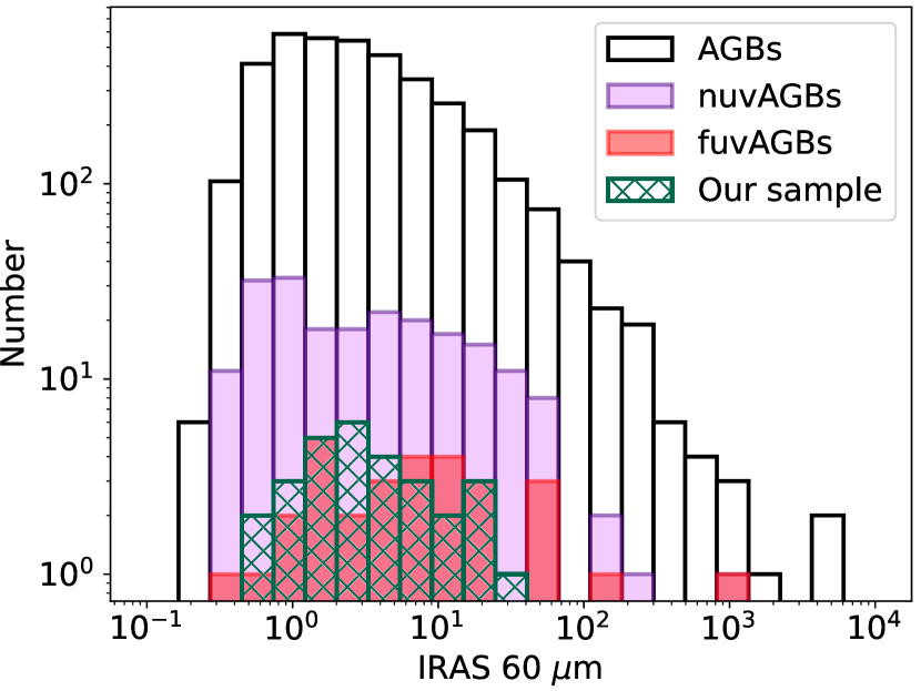
Figure 1: IRAS 60$\mu$m  flux distribution of our targets (green) and of AGB stars (including nuvAGBs and fuvAGBs) from Suh (2021), see Sect. 2. The colours represent the NUV/FUV emission; the sample is indicated in the top right corner for reference.

Figure 2 shows the IRAS [25-60] versus [12-25] two-colour diagram of the catalogue sources. The black lines present regions that contain sources with similar CSE properties and in a near evolutionary stage (for a detailed description, see van der Veen & Habing, 1988).

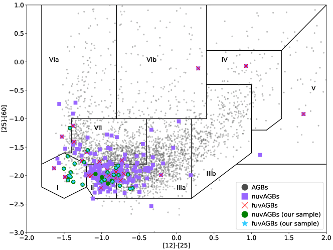
Figure 2: IRAS [25]-[60] vs [12]-[25] colour-colour diagram showing the location of our sample of 29 uvAGBs and the AGB stars (with and without UV excess) from the catalogue by Suh (2021), see Sect. 2. The colours of the markers represent the NUV–FUV emission; the sample is indicated in the bottom right corner for reference.

The majority of nuvAGBs and fuvAGBs are found in regions I, II, IIIa, or VII. Specifically, fuvAGBs tend to be concentrated in areas characterised by low values of [25]-[60] and [12]-[25] IRAS colours, primarily in regions I and II. This indicates that UV emissions are more prevalent in AGB stars with thin envelopes (see e.g. van der Veen & Habing, 1988). Given that our uvAGB sample primarily consists of fuvAGBs, their distribution also aligns with the concentration in regions I and II observed in the Suh (2021) catalogue of fuvAGBs.

The sample used in this work includes objects with different types of variability according to the General Catalogue of Variable Stars (GCVS, Samus’ et al., 2017) classification: 21% are Miras (M), 55% are semi-regular (SRs), and 24% are irregulars (LBs) as shown in table 2. Since most of the objects in our sample (25/29) have FUV+NUV emission, we compare the variability properties of our FUV+NUV sample with the FUV+NUV emitting AGB stars of the Suh (2021) catalogue, and find that the proportions of M, SRs and LBs are similar. However, for AGB stars with only NUV emission in the Suh (2021) catalogue, we find the proportions of SRs and LBs are much lower (23% and 13% respectively), and that Miras are most abundant (62%). FUV+NUV emission is more likely associated with binarity (and related accretion activity) than only NUV emission as shown in Sahai et al. (2022). Thus, our finding above that there are larger fractions of SRs and LBs in a sample of AGB stars with FUV+NUV emission compared to one with only NUV emission, suggests that SR and LB variability in AGB stars is an indicator of binarity.

However, further investigations using larger samples are needed to explore this tentative result more thoroughly, taking into account the observational bias that large samples likely cover a larger distance range. This makes it more difficult to detect and classify variability as well as to detect UV emission.

There are some targets in our sample that show low luminosities $\lesssim 3000L_{\odot}$ (see table 2). These low values are not expected for stars on the tip of the AGB. Therefore, it is possible that some of these low-luminosity sources are still on the Red Giant Branch (RGB) or in the early-AGB phase, and therefore have relatively low mass-loss rates with the result that they have not developed a detectable CSE (in millimetre-wave CO lines) as yet. Some of these low luminosities could potentially be attributed to distance inaccuracies.

3 Observations

The observations presented in this paper were carried out with the IRAM-30 m radiotelescope (Pico Veleta, Granada, Spain) using the Eight MIxer Receiver (EMIR, Carter et al., 2012) spectral line receiver. Observations were taken in two observational campaigns in 2009 and 2010.

We simultaneously observed the ¹²CO ($J$=2–1)(230.538 GHz) and ¹²CO ($J$=1–0)(115.271 GHz) rotational transitions with E090 and E230 receivers operated in dual sideband (2SB) mode and dual (H+V) polarisation. Observations were performed with different backends simultaneously. In this work, we present only the spectra taken with the VErsatile SPectrometer Array (VESPA), which provides the best spectral resolution of $\sim$0.3 MHz ($\sim$0.4 and 0.8 km s^-1 at 1 and 3 mm, respectively) over a spectral bandwidth of $\sim$216 MHz.

Observations were performed in wobbler-switching mode with a wobbler throw of 120″ and frequencies of 0.5 Hz. Calibration scans on the standard two load system were taken every $\sim$10-15 min. Pointing and focus were checked regularly on nearby continuum sources. After pointing corrections, the typical pointing accuracy was $\sim$2″-5″. On-source integration times are in the range 1-7.5 h (with a mean value of 1.7 h) per target.

The observation were reduced using CLASS following standard procedures, which include killing bad channels (if any), subtracting baseline, and averaging individual good-quality scans to produce the final spectra. For the sources observed in both the 2009 and 2010 observation campaigns (Y Crb, RW Boo, RU Her, DF Leo, OME Vir), the two epoch spectra were averaged after weighting by the inverse square of the rms noise of each individual spectrum. We present the spectra in the corrected antenna-temperature ($T^{*}_{\rm A}$) scale, which can be converted to main-beam temperature ($T_{\rm MB}$) applying the well-known relation $T_{\rm MB}$=$T^{*}_{\rm A}$/$\eta_{\rm eff}$, where $\eta_{\rm eff}$ is the main-beam efficiency. For the IRAM-30 m antenna $\eta_{\rm eff}$ $\sim$0.83 at 115 GHz and $\eta_{\rm eff}$ $\sim$0.65 at 230 GHz. The point source sensitivity (S/$T^{*}_{\rm A}$, i.e. the K-to-Jy conversion factor) is $\sim$6.01 and $\sim$7.89 at 115 and 230 GHz, respectively. The half-power-beam width (HPBW) of the IRAM-30 m antenna is 21$.\!\!^{\prime\prime}$4 at 3mm and 11$.\!\!^{\prime\prime}$7 at 1mm.

The noise of the spectra for a velocity resolution of 0.8 km s^-1 is in the range rms=7.7-95 mK (with a median value of 12 mK) at 1mm and rms=5-30 mK (with a median value of 11 mK) at 3mm. The uncertainty of the relative calibration of our observations was estimated by observing CW Leo, a well-studied AGB star with intense CO emission that is commonly used as a line calibration standard. The relative calibration uncertainty has also been checked by comparing the ¹²CO ($J$=2–1) and ¹²CO ($J$=1–0) spectra of five of our targets observed in 2009 as well as in 2010. Based on this, we estimate total line flux uncertainties of $\sim$20-25% at 1mm and of $\sim$10-15% at 3mm.

4 Observational results

We have searched for ¹²CO ($J$=1–0)   and ¹²CO ($J$=2–1)   emission in a sample of 29 uvAGB binary candidates. Line emission was detected in 15 targets, 11 of them in both transitions. The observed spectra are presented in Figs. 3 and 4 for ¹²CO ($J$=2–1)  and ¹²CO ($J$=1–0)  respectively. The main line measurements directly obtained from the observations are summarised in Table 5.

4.1 Line profiles and expansion velocities

The line profiles observed in our targets exhibit a range of shapes, including (pseudo) parabolic, double-horned, flat, triangular, Gaussian-like profiles, etc. Some objects also show profile asymmetries, such as horns with different intensities or quasi-triangular profiles with one side, in some cases the red-shifted one, being less intense. In the case of RW Boo, a double-component profile has been found as it had been previously reported by Díaz-Luis et al. (2019). The observed line profiles in our predominantly O-rich targets do not closely resemble the canonical profiles expected for the so-called standard CSE model, which assumes isotropic flow at a constant velocity. In the standard model, the line profile can vary between parabolic, flat, and double-horned shapes, depending on the line optical depth and the size of the envelope relative to the telescope beam (Olofsson et al., 1993). However, this deviation from the idealised CSE model is a known property of O-rich CSEs, as discussed in previous studies by Margulis et al. (1990); Knapp et al. (1998). These deviations can be attributed to geometric or velocity effects in the CSEs or multiple mass-loss components.

The ¹²CO ($J$=2–1) and ¹²CO ($J$=1–0) line profile have enabled us to estimate two key line parameters: the integrated flux and the average expansion velocities of the envelopes. These parameters were determined by fitting a shell-type profile using the software CLASS where the line shape is parametrised as

$$f(\nu)=\frac{A}{\Delta\nu}\frac{1+4H[(\nu-\nu_{0})/\Delta\nu]^{2}}{1+H/3},$$ (1)

where $A$ is the integrated area, $\nu_{0}$ is the central frequency, $\Delta\nu$ is the full width at zero intensity, and $H$ is the horn-to-centre ratio of the line. The equivalent expansion velocity is

$$\mbox{$V_{\rm exp}$}=c\frac{\Delta\nu/2}{\nu_{0}},$$ (2)

where $c$ is the speed of light.

Additionally, we determined the full width at half maximum (FWHM) of the lines by fitting a Gaussian profile to each detected transition. For RW Boo, the ¹²CO ($J$=2–1) and ¹²CO ($J$=1–0) lines exhibited a complex structure. In this case, the expansion velocities were estimated by combining two shell profiles: the primary component represented a two-horn profile, while the secondary component corresponded to a parabolic profile.

The line parameters derived as just described are listed in Table 5. The distribution of expansion velocities for our targets is depicted in Figure 6. The majority of the sources exhibit moderate expansion velocities ($V_{\rm exp}$ $\sim$ 10 km s^-1), which aligns with typical values observed in AGB stars. A few sources display narrower line profiles, indicating lower expansion velocities ($V_{\rm exp}$ $\lesssim$ 5 km s^-1). These specific sources include R Uma, RZ Uma, Z Cnc (identified only in the ¹²CO ($J$=2–1) transition), and Y Crb (identified in both lines).

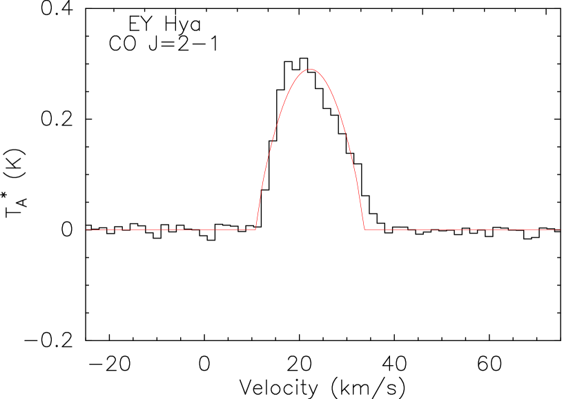
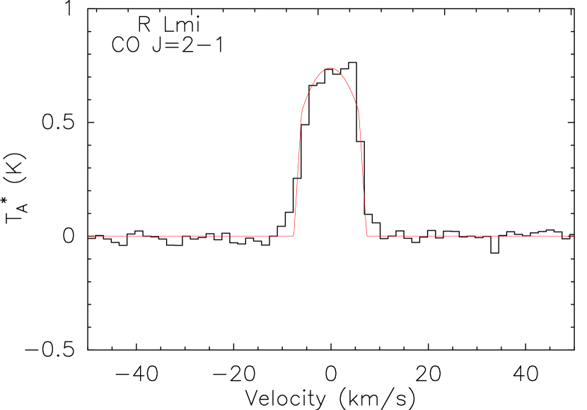
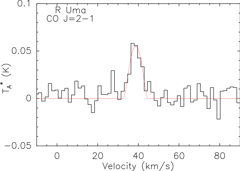
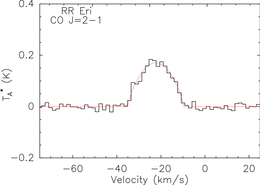
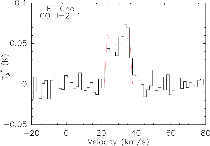
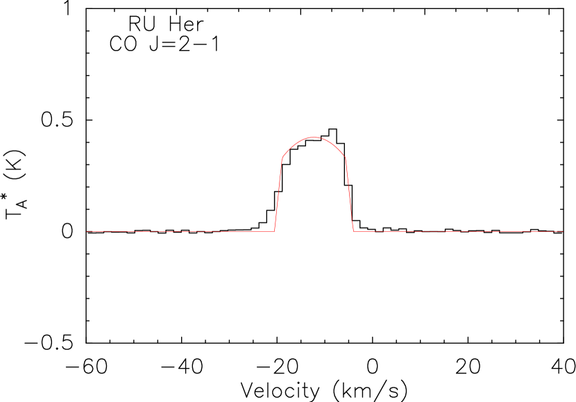
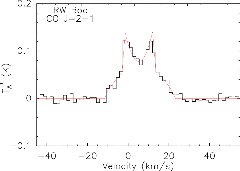
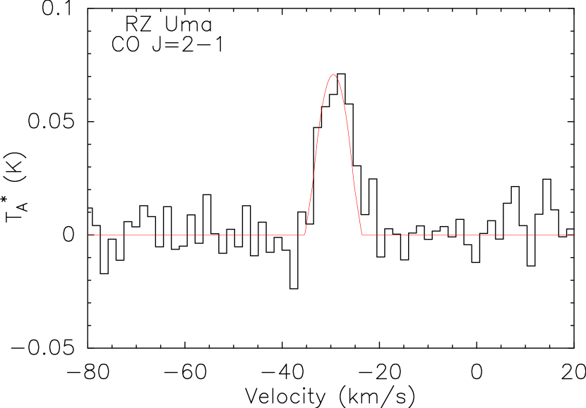
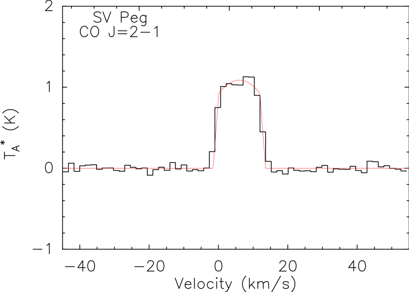
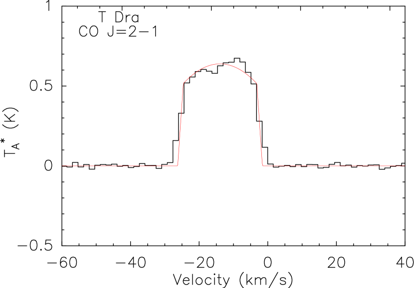
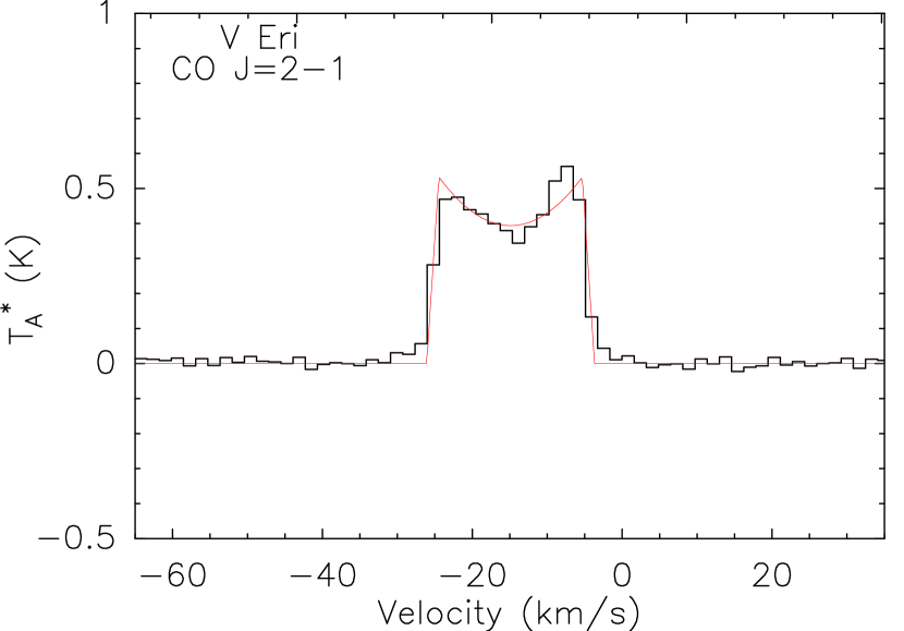
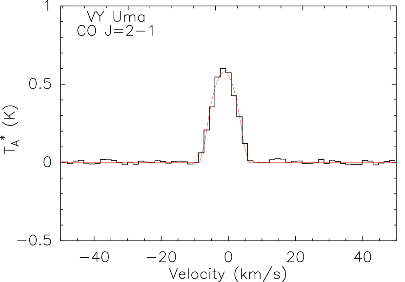
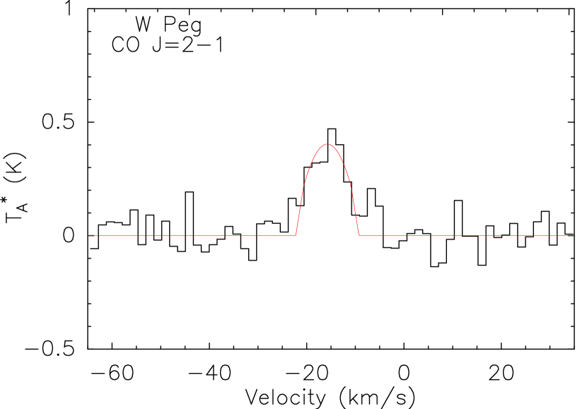
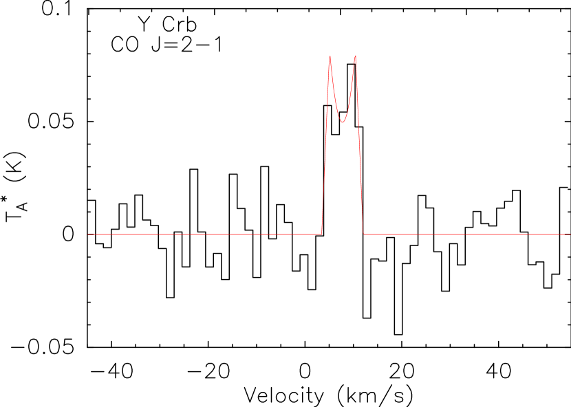
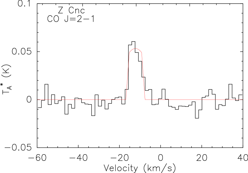
Figure 3: IRAM-30 m spectra of the 15 sources detected in the ¹²CO ($J$=2–1)  transition (velocity resolution is $\delta$v=1.6 km s^-1). Line profile fits are shown in red (see Sect. 4).

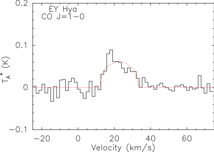
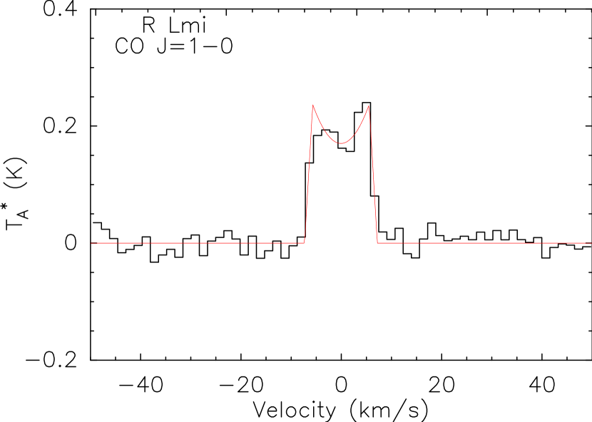
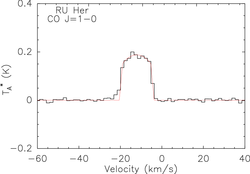
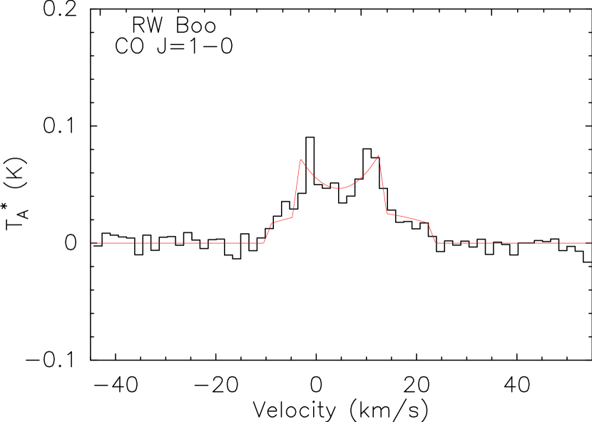
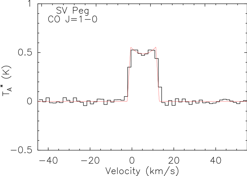
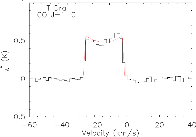
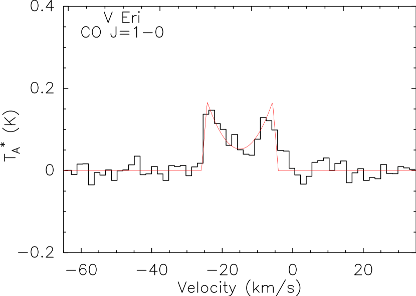
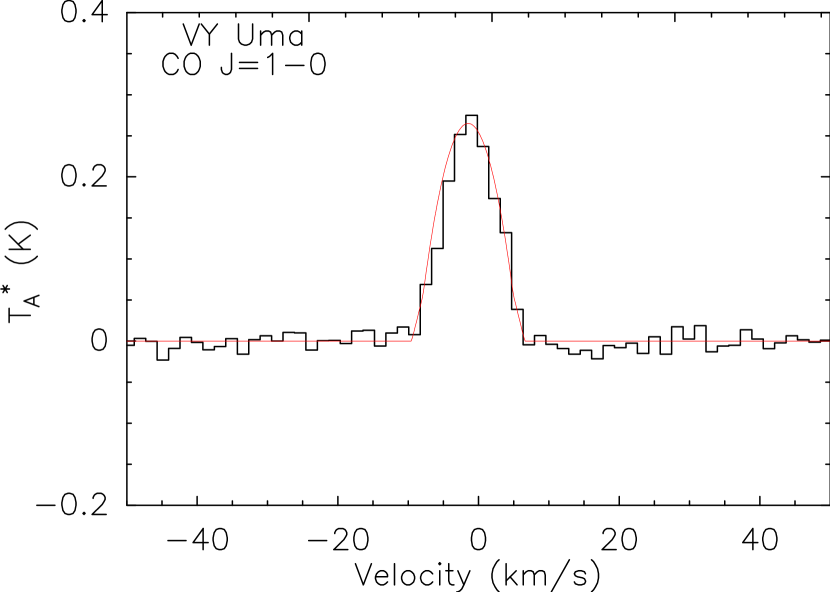
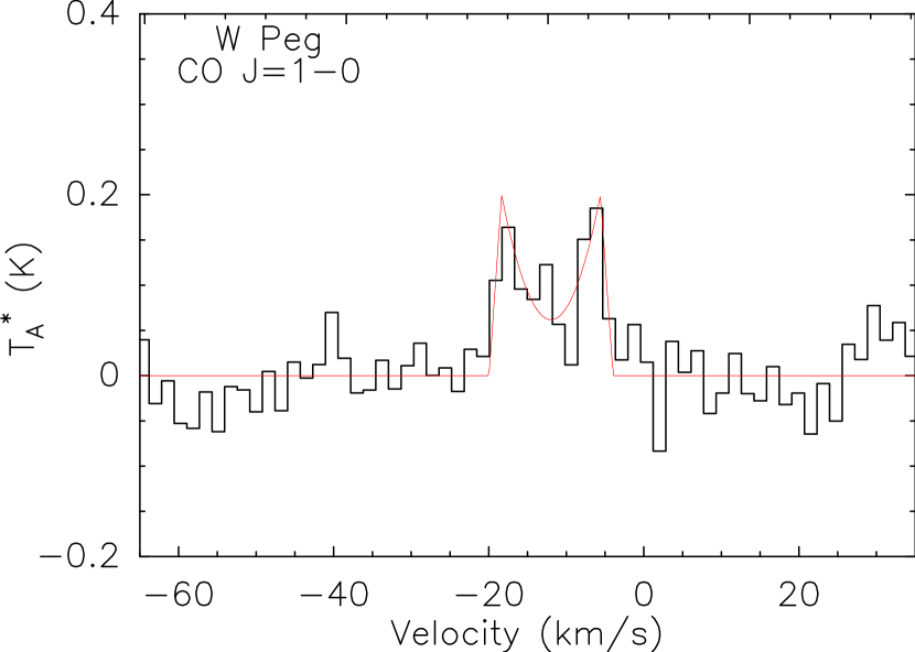
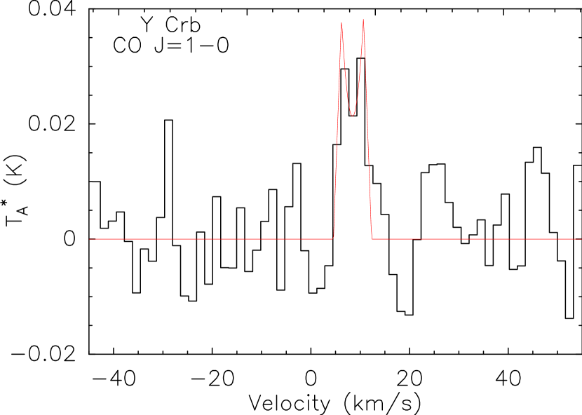
Figure 4: same as Fig. 3 for the 10 sources detected in the ¹²CO ($J$=1–0)  transition.

[b] Source line $\int T_{A}^{*}dv$ $\mathrm{T_{A}}$ rms $\mathrm{V_{sys}}$ $\mathrm{V_{exp}}$ FWHM $(\mathrm{K\,km\,s^{-1}})$ $(\mathrm{mK})$ $(\mathrm{mK})$ $(\mathrm{km\,s^{1}})$ $(\mathrm{km\,s^{1}})$ $(\mathrm{km\,s^{-1}})$ EY Hya ¹²CO ($J$=1–0) $1.12\pm 0.10$ $62$ $11$ $-24.6$ $10.1$ $14.7$ EY Hya ¹²CO ($J$=2–1) $4.74\pm 0.07$ $290$ $7$ $-21.5$ $10.7$ $14.6$ R Lmi ¹²CO ($J$=1–0) $2.42\pm 0.18$ $166$ $18$ $-1.7$ $6.4$ $11.6$ R Lmi ¹²CO ($J$=2–1) $9.5\pm 0.2$ $740$ $20$ $-2.0$ $6.7$ $11.2$ R Uma ¹²CO ($J$=1–0) $<0.22$ $12$ R Uma ¹²CO ($J$=2–1) $0.40\pm 0.09$ $50$ $9$ $-39.0$ $4.7$ $6.2$ RR Eri ¹²CO ($J$=1–0) $<0.72$ $15$ RR Eri ¹²CO ($J$=2–1) $2.94\pm 0.09$ $171$ $9$ $22.4$ $12.0$ $16.0$ RT Cnc ¹²CO ($J$=1–0) $<0.44$ $9$ RT Cnc ¹²CO ($J$=2–1) $0.76\pm 0.08$ $47$ $8$ $-33.0$ $7.2$ $11.7$ RU Her ¹²CO ($J$=1–0) $2.77\pm 0.05$ $187$ $5$ $12.2$ $7.6$ $12.8$ RU Her ¹²CO ($J$=2–1) $6.19\pm 0.06$ $422$ $6$ $12.0$ $7.5$ $12.7$ RW Boo ¹²CO ($J$=1–0) $1.29\pm 0.05$ $38$ $5$ $-5.1$ $17.3$ $20.3$ $3$ $7.7$ RW Boo ¹²CO ($J$=2–1) $2.07\pm 0.06$ $54$ $6$ $-4.4$ $15.6$ $19.8$ $29$ $8.4$ RZ Uma ¹²CO ($J$=1–0) $<0.26$ $11$ RZ Uma ¹²CO ($J$=2–1) $0.53\pm 0.10$ $66$ $10$ $28.6$ $4.7$ $7.7$ SV Peg ¹²CO ($J$=1–0) $7.48\pm 0.19$ $507$ $19$ $-5.3$ $7.3$ $12.5$ SV Peg ¹²CO ($J$=2–1) $13.9\pm 0.4$ $1120$ $40$ $-5.4$ $7.2$ $11.3$ T Dra ¹²CO ($J$=1–0) $12.1\pm 0.2$ $490$ $20$ $13.2$ $12.0$ $20.8$ T Dra ¹²CO ($J$=2–1) $14.18\pm 0.10$ $639$ $10$ $13.9$ $11.5$ $19.4$ V Eri ¹²CO ($J$=1–0) $2.29\pm 0.17$ $53$ $17$ $14.1$ $10.1$ $22.9$ V Eri ¹²CO ($J$=2–1) $9.55\pm 0.11$ $393$ $11$ $15.6$ $10.4$ $19.3$ VY Uma ¹²CO ($J$=1–0) $2.52\pm 0.10$ $256$ $11$ $1.2$ $6.7$ $8.5$ VY Uma ¹²CO ($J$=2–1) $5.14\pm 0.10$ $579$ $10$ $0.9$ $6.5$ $8.0$ W Peg ¹²CO ($J$=1–0) $1.9\pm 0.3$ $80$ $30$ $15.7$ $7.7$ $16.3$ W Peg ¹²CO ($J$=2–1) $4.0\pm 0.7$ $370$ $70$ $16.6$ $7.1$ $9.9$ Y Crb ¹²CO ($J$=1–0) $0.15\pm 0.08$ $21$ $8$ $-6.9$ $3.1$ $6.0$ Y Crb ¹²CO ($J$=2–1) $0.33\pm 0.15$ $58$ $16$ $-4.3$ $3.9$ $6.0$ Z Cnc ¹²CO ($J$=1–0) $<20$ $10$ Z Cnc ¹²CO ($J$=2–1) $0.42\pm 0.08$ $55$ $8$ $9.3$ $3.9$ $6.7$ • Notes. Column (1): source, Col. (2): transition, Col. (3): area of the observed line profil, Col. (4): antenna temperature at the central velocity of the fit to the line profile, Col. (5): noise, Col. (6): Systemic velocity (line centroid) in the local standard of rest (LSR) frame, Col. (7): expansion velocity of the shell fit, Col. (8): Full Width at a Half Maximum of the Gaussian fit.

Table 3: Spectral measurements for detected sources.

4.2 CO detection statistics

Regarding the variability type, in terms of CO detection fractions, we observed the following trends: 83% for Miras, 56% for SRs, and 14% for LB. These ratios are slightly lower compared to previous CO surveys of AGBs, where detection rates were around 90% for Miras, 70% for SRs, and 50% for LB (see e.g. Margulis et al., 1990; Kerschbaum & Olofsson, 1999). This effect, which is particularly notable for LB stars, could suggest that stars with UV excess have a lower likelihood of having CO-rich circumstellar envelopes compared to normal AGB stars. However, the relative order of detection ratios among the variability classes remains consistent.

The CO detection statistics is 50% (13/26) among O-rich stars and 100% (2/2) among C-rich stars. Since our sample is strongly biased towards O-rich stars, which represent 26 (90%) of the targets, the CO detection statistics depending on chemistry cannot be considered meaningful, although it does go in the same direction as in many previous works finding a larger CO detection fraction among C-rich AGB stars than in other chemistry types (e.g. Knapp & Morris, 1985).

Figure 5 illustrates the detectability of ¹²CO in our sample, highlighting the comparison between different parameters to identify any discernible trends. Figure 5 (a) shows that CO detections are not strongly biased towards the nearest targets, but spread over a wide range of distances between 300 and 1000 pc. In fact, there is a significant number of CO non-detections at distances lower than 300 pc.

Figure 5 (b) shows that the O-rich AGB stars of our sample located in regions I and VII were not detected, this is good agreement with the location of AGBs with thinnest CSEs in regions I or close to it (see van der Veen & Habing, 1988), whereas most of the targets located in region II and all the targets located in region IIIa were detected. On the other hand, the C-rich AGB stars of our sample were detected (VY Uma and T Dra, which are located in regions VIa and VII respectively).

In Sect. 7.1, we specifically examine the correlation between CO and IRAS flux. As anticipated, we observe a proportional relationship between these fluxes, consistent with most of the sources with CO detections being characterised by high IRAS brightness ($\mbox{F${}_{\rm 60}$}>5$ Jy). with the exception of Y Crb, which has $\mbox{F${}_{\rm 60}$}\sim 1.8$ Jy.

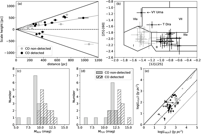
Figure 5: Comparison between different parameters and the ¹²CO detectability of our targets.
(a) Scale height vs distance for our targets. The solid line represents a viewing angle of $\pm 90^{\circ}$, the dotted line represents a viewing angle of $\pm 30^{\circ}$, and the dashed line represents a viewing angle of $0^{\circ}$. The non-detected in ¹²CO are shown as red circles, sources detected in ¹²CO ($J$=2–1)  line are shown as green squares, and sources detected in both ¹²CO lines are shown as blue stars.
(b) IRAS [25]-[60] vs [12]-[25] two-colour diagram restricted to those regions in which our sources are located (i.e. regions I, II, IIIa, VIa, and VII). The colour scheme is the same as (a).
(c) Histogram with the distribution of the NUV magnitudes of our sample. The sources detected in ¹²CO are shown in white and sources non-detected in ¹²CO are shown in grey.
(d) Same as (c) for FUV magnitudes.
(e) Comparison between NUV and FUV luminosities. The solid line represents the relation $R_{FUV/NUV}$=1, the dashed line represents the relation $R_{FUV/NUV}$=0.1, and the dotted line represents the relation $R_{FUV/NUV}$=0.01. Solid circles correspond to well measured luminosities and empty triangles to upper limits in one of the luminosities; the colour scheme is the same as (a).

Since the main difference between our sources and most AGB stars is their UV excesses, we have analysed the distributions of NUV and FUV magnitudes in relation with the CO detection. Figs. 5 (c) and (d) show the distributions of the NUV and FUV time-averaged magnitudes ($\rm M_{NUV}$ and $\rm M_{FUV}$ respectively) without reddening correction for the CO detected and non-detected sources. It is apparent that sources with CO detections have statistically higher UV magnitudes (lower UV fluxes) than those without CO detections. This difference is expected due to the fact that UV extinction is higher in envelopes with higher densities, we studied this anti-correlation with more detail in Sect. 6.

Figure 5 (e) illustrates the comparison between FUV and NUV luminosities ($L_{\rm FUV}$ and $L_{\rm NUV}$, respectively) without reddening correction for CO detections and non-detections. The relationship between the two, NUV and FUV, luminosities appears to be proportional, consistent with previous studies (see fig. 4 of Ortiz et al., 2019). However, some sources observed at different epochs exhibit variations that deviate from this correlation. These variations result in significant changes in the $R_{FUV/NUV}$ ratio, with some sources showing an increase in one flux and a decrease in the other. Moreover, the sources with highest GALEX luminosities (i.e BD Cam and Y Gem) also show a high $R_{FUV/NUV}$ ratio ($R_{FUV/NUV}$ $>$ 0.2), whereas our entire sample cover a range $R_{FUV/NUV}$ $\simeq$ 0.06-1.0. Without ignoring these considerations, the distribution does not reveal a clear trend between CO detections and the FUV/NUV ratio. However, it is evident that CO detections are predominantly found among sources with lower UV excess, as already deduced from Figs 5 (c) and (d).

5 Analysis: CO population diagrams

The main goal of this work is to characterise the molecular envelopes of uvAGB stars (i.e. AGB binary candidates) as a class. In this section we present our data analysis methodology to constrain the most relevant envelope parameters, including the mass-loss rate of the AGB wind, and the results obtained.

The CO rotational lines provide a fundamental diagnostic of the physical conditions of the molecular gas. As a first approximation, we have applied the classical population (or rotational) diagram method, explained in Goldsmith & Langer (1999), to estimate the beam-average excitation temperature ($T_{\rm ex}$) and the ¹²CO column density ($N_{\rm CO}$) of the CSEs layers where the ¹²CO ($J$=1–0)  and ¹²CO ($J$=2–1)  transitions observed are predominantly produced. This method has been successfully used in the analysis of the molecular emission from the envelopes of many evolved stars (e.g. Ramos-Medina et al., 2018; Justtanont et al., 2000).

The population diagram method relies on two main hypothesis: (i) optically thin emission and (ii) local thermodynamic equilibrium (LTE) conditions. As explained in Goldsmith & Langer (1999), under these two conditions, the column density of CO molecules in the upper state ($N_{\rm u}$) and its energy above the ground state ($E_{\rm u}$) are related by the following equation:

$$ln\,\frac{N_{u}}{g_{u}}=\ln\,\frac{3\mbox{$k_{\rm B}$}W}{8\pi^{3}\nu S_{\rm ul}\mu^{2}}=ln\,\mathrm{N}-ln\,C_{\tau}-ln\,\left(\frac{\Delta\Omega_{a}}{\Delta\Omega_{s}}\right)-ln\,Z-\frac{E_{u}}{k_{B}\mbox{$T_{\rm ex}$}}.$$ (3)

Here $g_{u}$ is the degeneracy of the upper level, Z is the partition function of the molecule, $k_{\rm B}$  the Boltzmann constant, $\nu$ is the rest frequency of the transition, S_ul is the line strength and $\mu$ is the permanent dipole moment of the molecule, $\mathrm{N}$ is the column density of the molecule (in our case ${N_{\rm CO}}$), $W=\int T_{A}^{*}dv$ is the integrated area of each spectral line, and $\Delta\Omega_{\rm a}$ and $\Delta\Omega_{\rm s}$ are the antenna and the source solid angle, respectively. The beam filling factor, defined as the ratio $(\Delta\Omega_{a}/\Delta\Omega_{s})$, has been estimated assuming a Gaussian distribution for both the antenna beam pattern and the source brightness distribution. Eq. 3 also incorporates the so-called opacity correction factor defined by Goldsmith & Langer (1999) as $C_{\tau}=\frac{\tau}{1-e^{-\tau}}$, where $\tau$ is the line peak optical depth. As discussed by these and other authors, this correction is valid as long as the lines are not very opaque ($\tau\lesssim 1$), which is the case of our sources (see below in this section).

According to Eq. 3, a straight-line fit to the points in the population diagram provides $T_{\rm ex}$ from the slope of the fit and $N$ from the y-axis intercept. The total CO column density has been converted to the total (H₂) mass in the CO-emitting volume for our targets in a simplified way as

$$\mathrm{M}=\mathrm{m_{H_{2}}}\Omega_{s}D^{2}\frac{N_{\rm CO}}{\mbox{$X_{\rm CO}$}},$$ (4)

where $\mathrm{m_{H_{2}}}=3.32\times 10^{-27}$ kg is the mass of the $\mathrm{H}_{2}$ molecule and $\mbox{$X_{\rm CO}$}=N_{\rm CO}/N_{\rm tot}$ is the ¹²CO-to-H₂ fractional abundance, assumed to be $\mbox{$X_{\rm CO}$}=2\times 10^{-4}$ for O-rich stars and $\mbox{$X_{\rm CO}$}=8\times 10^{-4}$ for C-rich stars (Ramos-Medina et al., 2018; da Silva Santos et al., 2019). Assuming constant expansion velocity and using the values of the total emitting mass, we calculate the mass-loss rates ($\dot{M}$) for each source in a simplified manner dividing the total mass by the crossing time of the CO-emitting layers, which is computed as the ratio between the characteristic radius of the CO envelope and the expansion velocity ($\mathrm{t_{exp}}=\mbox{$R_{\rm s}$}/$$V_{\rm exp}$).

The extent of the ¹²CO ($J$=1–0) and ¹²CO ($J$=2–1) emitting region in our targets is unknown a priori; however, it is a critical parameter to constrain the main envelope properties ($T_{\rm ex}$ and $N$) using the population diagram technique described above. In this work, we have obtained a self-consistent estimate of the mass-loss rate and of the characteristic radius ($R_{\rm s}$), considering that, as empirically demonstrated by Ramstedt et al. (2020), $R_{\rm s}$ is approximately 2-3 times smaller than the CO photodissociation radius ($R_{\rm CO}$) as obtained following the formulation by Mamon et al. (1988). We follow an iterative population diagram fitting process, starting by adopting a first value of $R_{\rm s}$  as input to derive a first guess of $\dot{M}$ (computed as described above). This value of $\dot{M}$ is then used to estimate $R_{\rm CO}$, which is given by

$$\mbox{$R_{\rm CO}$}=7.3\times 10^{16}\left(\frac{\dot{M}}{10^{-6}}\right)^{0.58}\left(\frac{10}{\mbox{$V_{\rm exp}$}}\right)^{0.4}\left(\frac{\mbox{$X_{\rm CO}$}}{4\times 10^{-4}}\right)^{0.5},$$ (5)

following the formulation by Mamon et al. (1988) (see also Planesas et al., 1990). This new value of $R_{\rm CO}$ is used to compute a new value of $R_{\rm s}$, which is then used as a new input value to derive again $T_{\rm ex}$, $N$, and $\dot{M}$. This process is repeated until the input and output $R_{\rm s}$  converge to the same value.

The population diagrams of our sources, with the corresponding linear fits obtained once the iterative process we have just described has converged, are plotted in appendix E. The values of the different envelope parameters derived are given in Table 4 and presented and discussed in the next section. For sources where only the ¹²CO ($J$=2–1)  transition is detected, the column density has been estimated assuming an excitation temperature of 10 K, which is similar to the mean value of $T_{\rm ex}$ derived for targets with detections in both ¹²CO ($J$=2–1)  and ¹²CO ($J$=1–0). However, in the case of RR Eri, the ¹²CO ($J$=2–1) /¹²CO ($J$=1–0)  line ratio was not consistent with $T_{\rm ex}$=10 K but indicated a higher value of $T_{\rm ex}$=25 K that has then been adopted.

From our analysis, we found optical depth values $\tau<<1$ for all sources except for T Dra, VY Uma and Y Crb, for which the CO peak-line optical depth takes values close to one for the ¹²CO ($J$=2–1) line. In these cases, the corresponding opacity-correction factor applied to the envelope mass and, thus, to the mass-loss rate is still moderate, of $\sim 1.6$.

We conducted a comparison between our estimated mass-loss rates ($\dot{M}$) and those previously reported in the literature ($\dot{M}$_lit) for those sources for which this is possible (a total of 11 sources). Some of these prior estimations employed more detailed analysis, such as radiative transfer models. By examining this comparison, documented in Appendix D, we found that the $\dot{M}$ values presented in this paper exhibit good agreement with those from previous studies. Therefore, despite relying on an approximate method, the population diagram yields relatively accurate results. This can be attributed to the effetive thermalisation or near-thermalisation of CO molecules in the CSEs, along with the low to moderate CO line opacities in our targets (for a more extensive discussion on this matter see Ramos-Medina et al., 2018). We estimate that our $\dot{M}$ values are accurate within a factor of approximately 3-4.

Considering the typical values of the radius of the CO-emitting layers found for our targets and the corresponding distances, we estimate angular diamaters ranging from approximately 1$.\!\!^{\prime\prime}$2 to 10″, that is, smaller than the telescope beam ($\sim$22″  and 11″  at 3 and 1 mm, respectively). Only T Dra and SV Peg, which possess larger sizes compared to the other sources, may exhibit partial resolution within the telescope beam.

Table 4: Parameters estimated for the circumstellar envelopes.

[b] Source $\mathrm{T_{rot}}$ $\mathrm{N_{tot}}$ $\theta_{\rm s}$ $R_{\rm s}$ $R_{\rm CO}$ M $\dot{M}$ $\mathrm{v_{exp}}$ $\mathrm{t_{exp}}$ E(B-V) (CSM) $A_{V}$ (CSM) $(\mathrm{K})$ $(\mathrm{10^{16}cm^{-2}})$ $(^{\mathcal{{\prime\prime}}})$ $(\mathrm{10^{16}cm})$ $(\mathrm{10^{16}cm})$ $(\mathrm{10^{-4}M_{\odot}})$ $(\mathrm{10^{-7}M_{\odot}\,yr^{-1}})$ $(\mathrm{km\,s^{-1}})$ $(\mathrm{yr})$ (mag) EY Hya $13\pm 6$ $2.9\pm 1.0$ $2.3$ $1.5$ $3.7$ $2.7$ $5.8$ $10.4\pm 0.3$ $500$ 0.026 0.0084 T Dra $5.8\pm 1.2$ $11\pm 2$ $4.8$ $7.1$ $18$ $55$ $29$ $11.8\pm 0.3$ $1900$ 0.025 0.0081 R Lmi $15\pm 7$ $3.5\pm 1.3$ $3.4$ $1.5$ $3.7$ $3.0$ $4.2$ $6.6\pm 0.1$ $700$ 0.031 0.010 R Uma $10^{*}$ $3.0\pm 0.7$ $0.9$ $0.7$ $2.1$ $0.6$ $1.3$ $4.7\pm 0.4$ $500$ 0.027 0.0087 RR Eri $25^{*}$ $2.4\pm 0.1$ $1.9$ $1.1$ $2.9$ $1.2$ $4.1$ $12.0\pm 0.3$ $300$ 0.022 0.0071 RT Cnc $10^{*}$ $1.5\pm 0.2$ $1.3$ $0.5$ $1.3$ $0.15$ $0.7$ $7.2\pm 0.2$ $200$ 0.013 0.0042 RU Her $8\pm 2$ $5.7\pm 1.5$ $2.8$ $3.0$ $7.6$ $20$ $16$ $7.5\pm 0.1$ $1300$ 0.051 0.017 RW Boo^† $6.0\pm 1.2$ $2.2\pm 0.7$ $2.7$ $1.1$ $2.6$ $1.0$ $3.5$ $12.3\pm 1.2$ $300$ 0.020 0.0065 RW Boo¹ $7.7\pm 1.2$ $1.6\pm 0.7$ $1.4$ $0.5$ $1.3$ $0.2$ $0.8$ $8.0\pm 0.3$ $200$ 0.020 0.0065 RW Boo² $5.3\pm 1.2$ $1.9\pm 0.7$ $2.6$ $1.0$ $2.5$ $0.8$ $3.9$ $16.6\pm 0.9$ $200$ 0.020 0.0065 RZ Uma $10^{*}$ $2.5\pm 0.5$ $1.0$ $0.8$ $2.0$ $0.6$ $1.2$ $4.7\pm 0.3$ $500$ 0.022 0.0071 SV Peg $8\pm 2$ $5.6\pm 1.5$ $5.0$ $2.9$ $7.4$ $20$ $15$ $7.3\pm 0.1$ $1300$ 0.050 0.016 V Eri $14\pm 7$ $3.0\pm 1.1$ $3.4$ $1.5$ $3.8$ $2.7$ $5.9$ $10.2\pm 0.2$ $500$ 0.027 0.0087 VY Uma $7.5\pm 1.9$ $5.1\pm 1.1$ $3.0$ $1.9$ $4.8$ $6.9$ $2.0$ $6.6\pm 0.1$ $900$ 0.011 0.0035 W Peg $7\pm 2$ $3.4\pm 1.2$ $2.8$ $1.5$ $3.7$ $2.9$ $4.5$ $7.4\pm 0.3$ $600$ 0.030 0.0097 Y Crb $7\pm 3$ $3.0\pm 1.7$ $0.9$ $0.9$ $2.4$ $1.1$ $1.3$ $3.5\pm 0.4$ $800$ 0.027 0.0087 Z Cnc $10^{*}$ $2.0\pm 0.5$ $0.9$ $0.6$ $1.5$ $0.3$ $0.6$ $3.9\pm 0.2$ $500$ 0.018 0.0058 • Notes. Column (1): name of the source, col (2): excitation temperature, col (3): CO column density, col (4): source radius in arcseconds, col (6): source radius in cm, col (6): photodisociation radius in cm, col (7): mass of the circumstellar envelope, col (8): mass-loss rate, col (9): average expansion velocity, col (10): expansion time, Col (11): reddening produced by the CSM (see Sect. C). (*) Fixed temperature. ($\dagger$) estimated with an average RW Boo $V_{\rm exp}$. (1) estimated for the RW Boo low $V_{\rm exp}$component. (2) estimated for the RW Boo high $V_{\rm exp}$ component (see table 5), components (1) and (2) are shown for illustrative purposes and were not taken into account in the analysis.

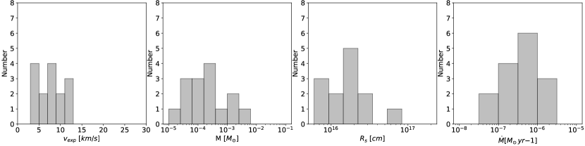
Figure 6: Distribution of the CO envelope expansion velocity ($V_{\rm exp}$), mass ($M$), characteristic radius ($R_{\rm s}$), and mass-loss rate ($\dot{M}$) of the uvAGB with CO detections in our sample.

6 Properties of the circumstellar envelopes

In this section, we will discuss the primary characteristics of the molecular envelopes surrounding our sample of uvAGB stars, which have been inferred from our detections of CO line emissions (Table 4). Furthermore, we will compare the obtained values with those derived from various AGB samples mentioned in the existing literature. In the case of RW Boo, we present the solution for the average $V_{\rm exp}$  as well as two additional solutions corresponding to each of the two $V_{\rm exp}$  components found in the spectral lines – these latter two solutions are presented for illustrative purposes, but were not taken into account in the posterior analysis.

Figure 6 presents the distributions of the key envelope parameters obtained in Sect. 5, specifically the expansion velocity ($V_{\rm exp}$), mass ($M$), characteristic radius of the CO-emitting volume ($R_{\mathrm{s}}$), and mass-loss rate ($\dot{M}$).

6.1 Expansion velocity

The distribution of expansion velocities in our sample exhibits a relatively even spread, encompassing values ranging from approximately 3 to 13 km/s (Fig. 6, left). These values fall within the range of expansion velocities observed in AGB envelopes, although they tend to occupy the lower part of the population, which typically reaches up to $\sim$30 km/s according to previous studies (Höfner & Olofsson, 2018). This outcome can be attributed to the composition of our sample, which primarily comprises O-rich AGB stars (90%) alongside a substantial proportion of irregular and semi-regular AGB stars (79%). It has been shown that O-rich have lower expansion velocities than C-rich AGBs (e.g. Margulis et al., 1990; Höfner & Olofsson, 2018). In addition, it is widely recognised that irregulars and semi-regulars exhibit systematically lower terminal velocities compared to Mira-type variables (see Olofsson et al., 2002).

The lowest expansion velocities observed in this study are those of the O-rich semi-regulars Y Crb and Z Cnc ($V_{\rm exp}$=3.5 and 3.9 km s^-1 respectively). According to Winters et al. (2003) the mass-loss mechanism in low outflow-velocity ($V_{\rm exp}$$<$5 km s^-1) AGB stars is fundamentally dominated by pulsations without the dust radiation pressure playing a dominant role, as opposed to the majority of AGBs. Another possibility is that the narrow profiles observed in some of our sources may be associated with stable, rotating structures in a circumbinary configuration, similar to what has been observed in L₂ Pup (see Kervella et al., 2019).

At the high end of our velocity distribution, with $V_{\rm exp}$ $\sim$12 km s^-1, we find the C-rich Mira T Dra and the O-rich semi-regulars RR Eri and RW Boo. For RW Boo a double-shell profile was found (see Sect. 4.1) indicating the presence of a slow ($V_{\rm exp}$$\sim$8.0 km s^-1) and a fast ($V_{\rm exp}$$\sim$16.6 km s^-1) wind components, in this analysis we have considered the parameters estimated with an average expansion velocity ($V_{\rm exp}$$=$12.3 km s^-1). Finally, within the sensitivity limit of our observations, we do not identify in any of the uvAGB stars in our sample the presence of massive, fast (up to a few hundred  km s^-1) molecular outflows like those commonly present in the subsequent evolutionary stages of pre-PN and PN (e.g. Bujarrabal et al., 2001; Sánchez Contreras & Sahai, 2012).

6.2 Size and mass

The characteristic radius of the envelope layers where the ¹²CO ($J$=1–0) and ¹²CO ($J$=2–1) emission observed is predominantly produced, which has been self-consistently estimated together with the mass-loss rate from our population diagram analysis (Sect. 5), takes values ranging from 6$\times 10^{\rm 15}$ cm to 2$\times 10^{\rm 17}$ cm with a mean around 2$\times 10^{\rm 16}$ cm. This is in good agreement with values obtained from previous works using similar empirical relationships or model-based indirect estimations (e.g. Groenewegen, 2017) but also from direct measurements from interferometric CO mapping (e.g. Ramstedt et al., 2020) for other samples of AGB CSEs with similar mass-loss rates.

The derived sizes of the envelopes and their corresponding expansion velocities indicate relatively short crossing or kinematical times, ranging from $\sim$200 to $\sim$2000 years (Table 4). Consequently, CO millimetre-wavelength observations are not sensitive to the mass-loss process that occurred more than a few thousand years ago. This finding aligns with the relatively low values of the envelope mass discovered in our study, ranging from $10^{-5}$ to $5\times 10^{-3}$ $M_{\odot}$, with a peak around $3\times 10^{-4}$ $M_{\odot}$. Our analysis reveals a slightly higher mass distribution compared to the results reported by Ramos-Medina et al. (2018) and da Silva Santos et al. (2019) based on high-$J$ CO emission observations using the Herschel telescope. This discrepancy is consistent with the fact that far-infrared observations probe a smaller volume, closer to the central regions, compared to the millimetre-wavelength observations.

6.3 Mass-loss rate

The distribution of $\dot{M}$ of our sample covers a range from 6$\times 10^{\rm-8}$ to 3$\times 10^{\rm-6}$ $M_{\odot}$ yr^-1  with a mean value of 6$\times 10^{\rm-7}$ $M_{\odot}$ yr^-1. The mass-loss rates obtained in our study fall within the range of values reported in previous investigations of large samples of AGB stars (see Höfner & Olofsson, 2018). However, it is worth noting that our sample lacks objects exhibiting extremely high or extremely low mass-loss rates, specifically those reaching up to few$\times 10^{\rm-4}$ $M_{\odot}$ yr^-1 or falling below a few$\times 10^{\rm-8}$$M_{\odot}$ yr^-1. The uvAGB stars in our sample with the lowest and highest mass-loss rates are Z Cnc and T Dra, respectively.

For AGB stars there are well-known correlations between some of the fundamental parameters of their envelopes, in particular, between $\dot{M}$ and $V_{\rm exp}$ and between these and the stellar pulsation period ($P$) for regular and semi-irregular variables. In Fig.7 we explore those same relationships to see if they are followed in the same way for our sample of uvAGBs. In this comparison, we use the sample of AGB stars recompiled by Van de Sande et al. (2021). Pulsation periods for all targets (AGBs and uvAGBs) are obtained from General catalogue variable stars (GCVS).

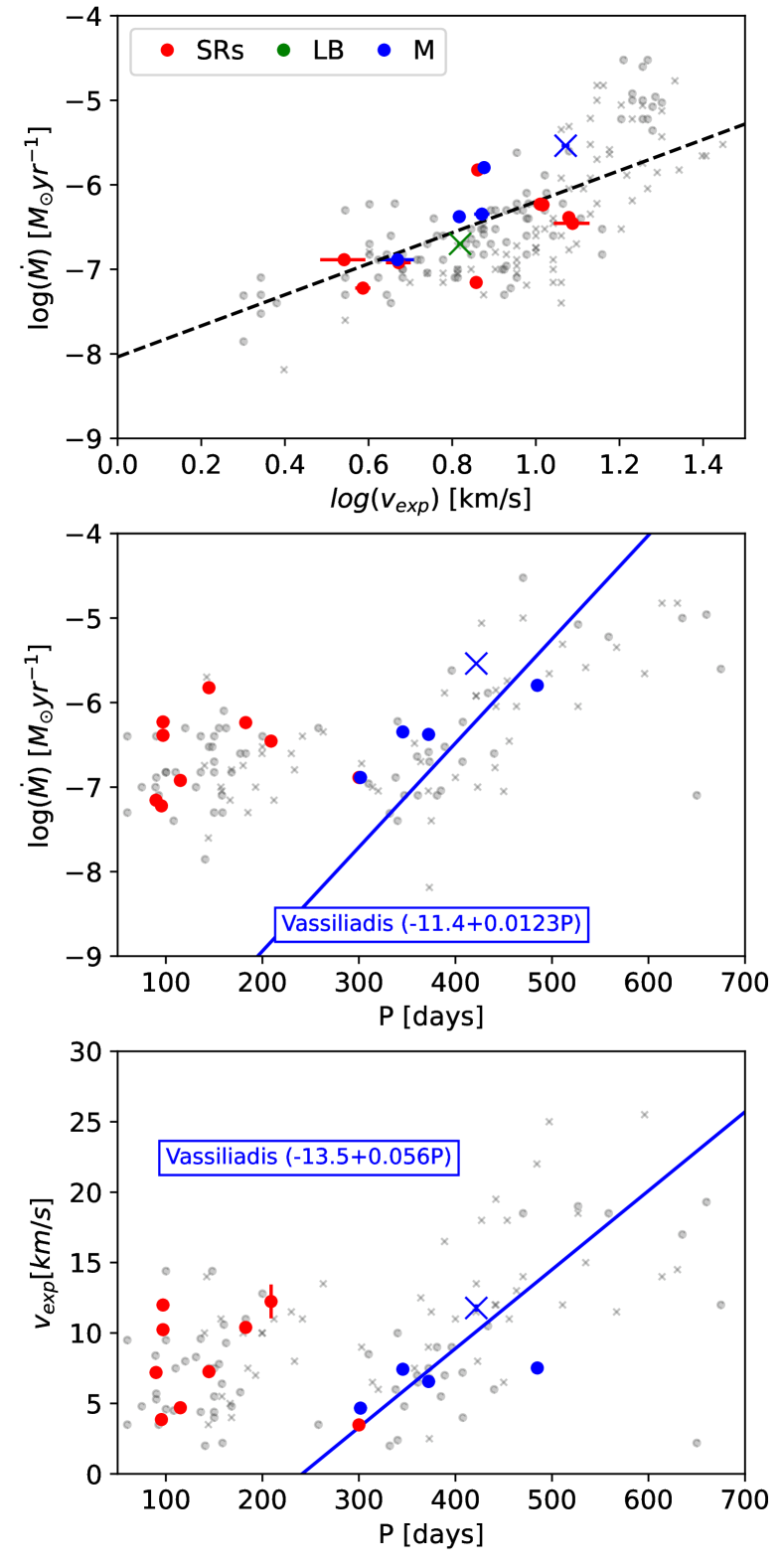
Figure 7: Comparison between some fundamental parameters of the AGBs envelopes ($\dot{M}$, $V_{\rm exp}$  and $P$) and with well-known correlations found in the literature. Upper: Relationship between $\dot{M}$  and $V_{\rm exp}$. Centre: Relationship between $\dot{M}$  and $P$. Lower: Relationship between $V_{\rm exp}$  and $P$. The colours of the markers represent the variability type. Red: semi-irregulars (SRs), green: irregulars (LB), and blue: Miras (M). The dashed line represents the linear fit performed over our sample and the solid lines represent the linear relationships for $\dot{M}$  and $V_{\rm exp}$  with $P$  found for Mira AGBs from Vassiliadis & Wood (1993). Grey markers represent AGB stars with $\dot{M}$ and $V_{\rm exp}$ values recompiled by Van de Sande et al. (2021). The shape of the markers represents the chemistry type in the two samples: circles for O-rich AGB stars and crosses for C-rich AGB stars.

The mass-loss mechanism primarily manifests itself through two key parameters: the mass-loss rate ($\dot{M}$) and the expansion velocity ($V_{\rm exp}$). Extensive studies on large samples of AGB stars have consistently demonstrated a correlation between these parameters of the type $\dot{M}$  $\propto$ $V_{\rm exp}$^α with values of $\alpha$=1.4-3.3 depending on chemistry and variability type of the stars (see e.g. Young, 1995; Knapp et al., 1998; Olofsson et al., 2002). In our specific study of uvAGBs, we obtained a very similar result (Fig. 7, top) showing a weak relationship $\mbox{$\dot{M}$}\simeq 10^{-8}\mbox{$V_{\rm exp}$}^{1.8}$. However, it is important to note that our sample size is relatively smaller compared to previous studies, which may partially explain the relatively low Pearson’s correlation coefficient found, $r$=0.65. In line with previous findings by Olofsson et al. (2002), a weaker correlation between $\dot{M}$  and $V_{\rm exp}$  was observed for O-rich AGB stars when compared to their C-rich counterparts. The spread in the $\dot{M}$  versus $V_{\rm exp}$  trend found in previous studies of AGB stars is in any case large, which probably reflects dust-to-gas ratio variations among other factors (Netzer & Elitzur, 1993; Habing et al., 1994).

In the case of regular variable stars, such as Mira-type stars, it is widely recognised that a correlation exists between both $\dot{M}$ and $V_{\rm exp}$ and the stellar pulsation period, $P$ (e.g. Vassiliadis & Wood, 1993). The uvAGB stars in our sample adhere closely to this relationship, as depicted in Fig. 7 (middle and lower panels). The semi-regular uvAGB stars, however, tend to cluster in the low-period region ($P$$<$200 days), exhibiting mass-loss rates (and expansion velocities) in the range $\dot{M}$$\sim$10^-7-10^-6$M_{\odot}$ yr^-1 ($V_{\rm exp}$$\sim$5-15 km s^-1), which is greater than would be expected based on their relatively short periods if they were Mira variables. Notably, no discernible correlation with the period is observed for these semi-regular uvAGB stars, which aligns with findings from larger semi-regular AGB samples (Van de Sande et al., 2021). In these cases, it suggests that there is another influential factor, beyond pulsation, playing a significant role in governing the mass-loss process of these objects.

6.4 Mass outflow momentum and $\dot{M}$-$L_{\rm bol}$ relationship

In our study of uvAGBs, we have examined the ratio $\beta$=$\dot{M}$ $V_{\rm exp}$ $c$/$L_{\rm bol}$, which compares the momentum rate in the mass outflow ($\dot{M}$ $V_{\rm exp}$) to the momentum rate in the stellar radiation ($L_{\rm bol}$/$c$). This parameter, also known as the overpressure or radiation pressure efficiency, is directly proportional to the dust opacity of the wind if radiation pressure on dust grains is the main wind driving force (Knapp, 1986; Lefevre, 1989).

Analysing the distribution of beta values for our sample (Fig. 8, upper panel), we consistently find values well below 1 for all the sources, aligning well with the values observed in the majority of AGB stars and with the values expected if radiation pressure is the principal operative mechanism. As pointed out by Knapp (1986), the $\beta$ values much lower than 1 (found in our sample but also in some AGB stars) indeed suggests that these objects are not losing mass as efficiently as it is possible. It is worth mentioning also that while some AGB stars may exhibit $\beta$ values slightly higher than 1, which can be attributed to multiple scattering (Lefevre, 1989), none of the objects in our sample demonstrate such behaviour. The sources with the largest values of $\beta$$\sim$0.1-0.2 are T Dra and RW Boo. In the case of the progeny of AGB stars (i.e. post-AGBs or pre-PNe), it is frequently observed that the $\beta$ values are notably high, which is considered as an indication that a distinct mass-loss mechanism, one that differs from radiation pressure acting on dust, is occurring in these stages (Bujarrabal et al., 2001).

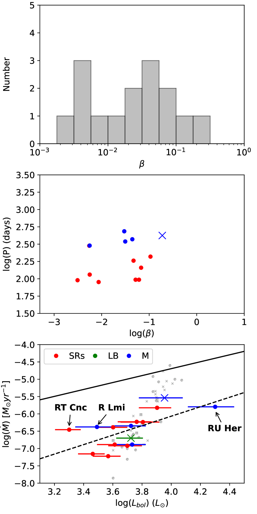
Figure 8: Comparison between envelope parameters related with the mass-loss mechanism. Upper: Distribution of the $\beta$ parameter, defined as the ratio of the outflow to the stellar radiation momentum ($\beta$=$\dot{M}$ $V_{\rm exp}$ $c$/$L_{\rm bol}$, Sect. 6.4). Centre: Relationship between stellar pulsation period ($P$) and $\beta$. Lower: Relationship between $\dot{M}$ and $L_{\rm bol}$ ; the solid line represents the single-scattering limit in the case $V_{\rm exp}$=10km s^-1  (see Groenewegen & Sloan, 2018) and the dashed line the best linear fit to our dataset. The colours and shapes of the markers are the same as in Fig. 7. Grey markers represent AGB stars with $\dot{M}$ and $L_{\rm bol}$ values recompiled from Danilovich et al. (2015) (circles: O-rich AGB stars, squares: S stars, and crosses: C-rich AGB stars).

Stellar pulsation is the other mechanism determining the mass-loss rate. We find a rough proportionality between $\beta$ and the pulsation period $P$ for our sample (Fig. 8, central panel), in agreement with previous results for AGB stars (Knapp, 1986). The observed trend reflects an underlying correlation between $\dot{M}$  and $P$: the mass-loss rate increases with longer periods and consequently, the dust opacity also increases. We find that Mira variables and semi-regulars occupy two distinct regions in the $P$-$\beta$ diagram. The SRs are located in the lower part, reflecting that despite their shorter periods, they exhibit similar mass-loss rates compared to Mira variables as shown in Fig. 7 (middle panel).

In the last panel of Figure 8, we conducted a comparison between $\dot{M}$ and $L_{\rm bol}$ for our sample. All our targets fall below the single-scattering limit, represented by the solid line, as already discussed and indicated by the low values of $\beta$ observed. We observed a correlation that can be described by the power-law relation $\mbox{$\dot{M}$}\sim 3\times 10^{-12}\mbox{$L_{\rm bol}$}^{1.4}$, represented by the dashed line in the figure. A power-law relationship is in line with expectations and is commonly observed in AGB stars. It indicates that as the luminosity increases, either due to larger stellar masses or a more advanced stage of evolution on the AGB, the mass-loss rate tends to increase as well (Höfner & Olofsson, 2018; Groenewegen & Sloan, 2018). We conducted a comparison between our values of $\dot{M}$ and $L_{\rm bol}$ with those reported by Danilovich et al. (2015), who estimated mass-loss rates from radiative transfer modelling of CO line emission in a sample of 53 AGB stars. Upon initial inspection, there is an apparent discrepancy in the exponent of the power-law relationship between the two samples. However, when considering the majority of sources in both studies, there is a general agreement and similarity in the distribution of points. The only notable exceptions are three objects (RT Cnc, RU Her, and, perhaps R LMi) located at the extreme high and low ends of the luminosity range. If we exclude these objects from the analysis, the slopes or power-law exponents of the correlations in both studies match more closely. This indicates that, overall, there is consistency between the mass-loss rate and luminosity relationships derived from our study and that of Danilovich et al. (2015), with the exception of a few outliers.

7 CO emission and CO-derived envelope parameters correlations with IR/UV properties

In this section we investigate correlations between the CO emission intensity and the infrared and ultraviolet continuum emission, as well as the bolometric luminosity. We also explore trends between the primary envelope parameters derived from CO and the distinctive ultraviolet emission properties exhibited by our targets.

7.1 CO versus IRAS 60$\mu$m emission

The correlation between CO line intensity and the IRAS 60$\mu$m emission has been well established for low-to-intermediate mass evolved stars, including AGB and post-AGB stars, as documented in numerous previous studies (Nyman et al., 1992; Bujarrabal et al., 1992; Olofsson et al., 1993, among others). This correlation is attributed to the fact that both the CO emission and the IRAS 60$\mu$m emission are indicative of the amount of material (in the form of gas and dust, respectively) present in their envelopes.

In our study of uvAGB stars, we also observe a strong correlation between the velocity-integrated luminosity of the ¹²CO ($J$=2–1) transition ($L_{\rm CO}$) and the IRAS 60$\mu$m luminosity ($L_{\rm 60\mbox{$\mu$m}}$) as shown in Fig. 9 (upper panel). This finding supports the notion that the gas and dust mass-loss rates are proportional to each other. Given that the infrared radiation is a significant or dominant component of the energy emitted by the dusty envelopes around AGB stars, it is reasonable to expect a correlation between the CO luminosity and the bolometric luminosity, which is in fact observed in our sample of uvAGBs (Fig. 9, central panel).

A linear fit to the $L_{\rm CO}$ versus $L_{\rm 60\mbox{$\mu$m}}$ and $L_{\rm bol}$ data points yields

$$L_{\rm CO}\approx 0.1\times 10^{1.2}L_{\rm 60\mbox{$\mu$m}},$$ (6)

$$L_{\rm CO}\approx 0.2\times 10^{2.0}\mbox{$L_{\rm bol}$}.$$ (7)

We note that most of the low-luminosity ($\mbox{$L_{\rm bol}$}<$3000 $L_{\odot}$) sources are CO non-detections (triangles in Fig. 9). Some of these low-luminosity targets could be RGB or early-AGB stars, with mass-loss rates still well below the maximum values reached at the tip of the AGB phase (see e.g. Höfner & Olofsson, 2018). However, the large uncertainties in their luminosities (see Sect. 2) does not allow us to robustly assert that these are not AGB stars. Nevertheless, they do not affect the posterior analysis as the CO non-detections were not used in the fitting; the derived upper limits on their CO fluxes are quite consistent with various relationships obtained for the detected targets discussed in this section (see e.g. the relationships between CO and IRAS 60$\mu$m/bolometric luminosities shown in Fig. 9).

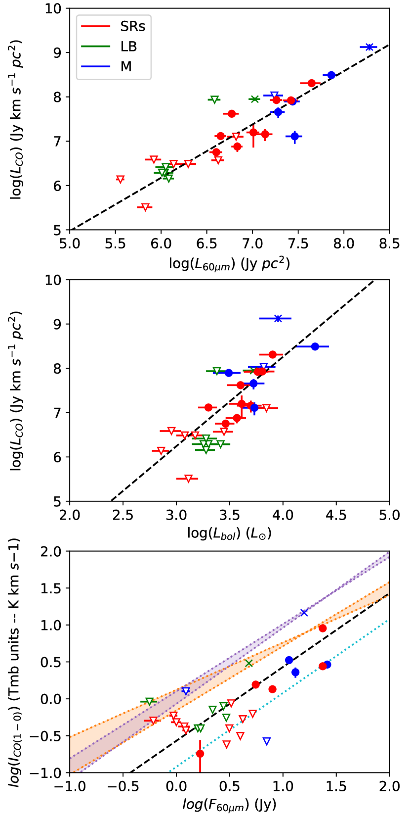
Figure 9: Comparisons of the CO integrated intensity, IRAS 60$\mu$m emission, and bolometric luminosity (Tables LABEL:tab:fluxes and 2). In the upper and middle panels $L_{\rm CO}$ is compared with $L_{\rm 60\mbox{$\mu$m}}$ and $L_{\rm bol}$. In the lower panel the ¹²CO ($J$=1–0) main-beam brightness temperature ($T_{\rm MB}$) is plotted against the IRAS 60$\mu$m flux after properly scaling $T_{\rm MB}$ when observed with a telescope other than the IRAM-30m antenna (see 7.1). The dashed line is the best linear fit to our data; the dotted lines are linear correlations from Nyman et al. (1992) and Bujarrabal et al. (1992) for O-rich AGBs (orange), C-rich AGBs (purple), and pre-PNe (cyan). The colours and shapes of the markers are the same as in Fig. 7.

In the literature, there are different approaches used by several authors to compare the relationship between the CO intensity and the IRAS 60$\mu$m emission. In principle, we focused on using the luminosity as a reference magnitude and specifically examined the ¹²CO ($J$=2–1) transition due to its higher number of detections compared to the ¹²CO ($J$=1–0)transition. However, a common method employed in exploring the CO-F₆₀ emission relationship is by comparing the main-beam brightness temperature ($T_{\rm MB}$ in K) of the ¹²CO ($J$=1–0) transition with the IRAS 60$\mu$m flux (in Jy). In Fig. 9, lower panel, we show the distribution of the uvAGBs in this study using this same representation together with the relationships derived for different samples of AGB stars in the past.

Specifically, we refer to the relationships presented in Nyman et al. (1992) for AGBs in different regions of the two colour IRAS diagram (the same regions are shown in Fig 2), including O-rich sources (located into regions II and III) and C-rich sources (located into regions VIa and VII). To account for the difference in beam size between the SEST 15m telescope, used as a reference in the studies of Nyman et al. (1992), and the IRAM 30m antenna, used in this work, we multiplied their relationships by a factor of 4 for a proper comparison with ours. Furthermore, we present the relationship described by Bujarrabal et al. (1992) for PPNe, which shows that PPNe are positioned noticeably below the relationships observed for AGBs. Bujarrabal et al. (1992) interpreted this as an indication that PPNe generally have a lower gas-to-dust mass ratio. This could be attributed to significant CO photodissociation in more advanced stages of evolution beyond the AGB phase, in which the envelopes become more diluted, and the central stars become hotter.

We found a relationship $I_{\rm CO}\sim 0.27\mbox{F${}_{\rm 60}$}$ for our sample of 10 targets with 1–0 detections (2 C-rich and 8 O-rich). The only two C-rich uvAGBs in our sample lie very close to the expectations based on the CO-F₆₀ relationship reported by Nyman et al. (1992) for this same chemical type. The O-rich uvAGBs in our sample, however, seem to fall below the relationship for O-rich AGBs (Nyman et al., 1992) and much closer to the relationship for PPNe (Bujarrabal et al., 1992). Since our uvAGBs are characterised by an excess of emission in the UV, this result does not seem overly surprising and could indicate, as in the case of PPNs, that a non-negligible fraction of the molecular gas is dissociated by the central source. We further discuss this in Section 8.1 in connection with the CO-to-UV relationship.

7.2 CO versus NUV and FUV emission

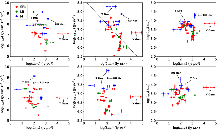
Figure 10: Comparisons between the ¹²CO ($J$=2–1) velocity-integrated luminosity ($L_{\rm CO}$, left), IRAS 60$\mu$m luminosity ($L_{\rm 60\mbox{$\mu$m}}$, middle), and bolometric luminosity ($L_{\rm bol}$) with the luminosity in the GALEX NUV and FUV bands (top and bottom panels, respectively). The colour-coding used for variability types is shown in the top left panel. Triangles are upper limits. The dashed line represents the best linear fit to the F₆₀-to-$L_{\rm NUV}$ data points (Pearson’s correlation coefficient r=-0.48). The trends in the rest of the variables represented have not been confirmed (§ 7.2).

A potential trend between the CO emission and the distinctive UV properties of uvAGB stars has not been explored before. For our sample, $L_{\rm CO}$ is compared with the extinction-corrected luminosities in the NUV and FUV bands ($L_{\rm NUV}$ and $L_{\rm FUV}$; see Fig. 10, left panels). As previously discussed in Sect. 4.2, the CO non-detections (indicated by triangles) tend to cluster towards the higher range of NUV and FUV luminosities, suggesting a potential inverse relationship between CO and UV intensity. Establishing a definitive trend is challenging, however, since the CO-NUV and -FUV diagrams exhibit a considerable spread, the number of CO detections is relatively small or moderate (15 sources) and (unlike CO) the UV emission is notably variable.

To address the limitation of a relatively small number of CO detections, and considering the established proportionality between CO and IRAS 60$\mu$m emission (discussed in Sect. 7.1), we also examine the relationship between UV and IRAS 60$\mu$m luminosity (Fig. 10, middle panels). In these diagrams, the presence of an anti-correlation appears to emerge more clearly but only for the NUV band, for which we derive a Pearson’s correlation coefficient of r=$-$0.48. For the FUV band, however, the anti-correlation is not confirmed (r=$-$0.01) as the CO intensities exhibit a significant spread (on the order of dex$\sim$2-3) for very similar values of $L_{\rm FUV}$.

In the right panels of Figure 10, we examine the relationship between the total bolometric luminosity and the NUV and FUV luminosity for our target stars. We tentatively observe a weak anti-correlation (r=$-$0.30) in the NUV band, which is likely influenced by the underlying $L_{\rm 60\mbox{$\mu$m}}$-to-$L_{\rm NUV}$ relationship. However, in the FUV band, no clear trend is evident. This observation aligns well with the results reported by Montez et al. (2017) in a comprehensive study of GALEX uvAGBs, where no significant correlation was found between FUV band emission and other bands ($UBVRIJHK$), in contrast to the stronger correlations observed in the NUV flux.

In all the diagrams presented and discussed above, we assigned different labels to our uvAGB stars based on their variability class to examine potential trends. However, no significant relationships were observed, except for the expected observation that Mira-type variables generally exhibit stronger CO emission compared to semi-regulars and irregulars, which is consistent with broader studies of AGB stars.

Finally, it is worth noting that the sources T Dra, RU Her and Y Gem stand out as outliers in all these diagrams, deviating from the general pattern observed in the sample. T Dra exhibits exceptionally intense CO and IRAS 60$\mu$m emission compared to the rest of the sample, yet its NUV and FUV emission falls within the average range. Similarly, RU Her shows the second more intense CO and IRAS 60$\mu$m emissions as well as the largest $L_{\rm bol}$, it also shows a large NUV flux despite the fact that it was not detected in the FUV band. In contrast, Y Gem is the strongest UV emitter in the sample, displaying also significant UV variations, and at the same time it shows relatively high values of $L_{\rm 60\mbox{$\mu$m}}$ (Even though, a weak ¹²CO ($J$=2–1) emission line was reported by Sahai et al., 2011). Remarkably, T Dra and Y Gem share an additional characteristic, they are both X-ray emitters. This X-ray emission perhaps suggests a more extreme nature for these uvAGB stars (potentially connected with strong binary interactions), warranting further investigation into the underlying mechanisms driving their distinct behaviour.

7.3 Envelope parameters versus NUV and FUV emission

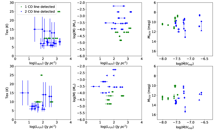
Figure 11: Comparison of main envelope parameters ($T_{\rm ex}$, M, and $\dot{M}$/$V_{\rm exp}$) and UV properties of our sample of uvAGBs (NUV and FUV; top and bottom panels, respectively).

In the investigation of potential trends between the two main envelope parameters derived from the CO population diagram analysis, namely the excitation temperature ($T_{\rm ex}$) and the mass in the CO-emitting volume (M), no clear correlation or trend was observed in any of the cases with any of the UV bands, as shown in the left and middle panels of Figure 11. However, it is important to consider two important factors that could make it challenging to identify a correlation even if it exists. Firstly, the small number of sources, particularly those with two detected lines, which provide more reliable values of $T_{\rm ex}$ and M. In this case, only 10 sources met the criteria, limiting the statistical power of the analysis. Secondly, the variability in the NUV and FUV bands introduces additional dispersion on the x-axis of the diagrams. This variability can obscure any underlying correlation between the envelope parameters and the UV bands.

There is an additional factor that introduces complexity in discerning a clear trend of the UV emission with the envelope temperature, which is the lower limit nature of $T_{\rm ex}$ derived from the CO population diagram analysis. This is because some regions in the outer layers of the envelope, where the low-$J$ CO transition emission originates, may reach densities close to, but slightly below, the critical densities of the CO 1–0 and 2–1 transitions (i.e. $\lesssim$(1-5)$\times 10^{\rm 4}$  cm^-3). Consequently, the derived $T_{\rm ex}$ values may underestimate the true $T_{\rm kin}$ of the gas.

Possible mild deviations from LTE are not anticipated to strongly impact the mass estimation. This has been discussed in detail by Ramos-Medina et al. (2018) and da Silva Santos et al. (2019). The reason for this is that even though $T_{\rm ex}$ may deviate from the true $T_{\rm kin}$, it precisely represents the level population distribution. As a result, the computation of the total number of emitting molecules (and hence, the mass) remains robust since it involves summing up the populations of all levels.

In our study, we also investigated the relationship between extinction-corrected GALEX magnitudes ($M_{\rm NUV}$ and $M_{\rm FUV}$) and $\dot{M}$/$V_{\rm exp}$ as a density proxy. We did not observe a confirmation of the linear anti-correlation depicted in Figure 10 of Montez et al. (2017) in the NUV band. However, it is important to note some differences between our study and that by Montez et al. (2017). First, we included GALEX UV photometry for different epochs when available. Second, we dereddened the GALEX magnitudes using distance-corrected values of the total extinction (interstellar and circumstellar, see tables 2 and 4), instead of relying on the default extinction estimate included in the GALEX catalogue, which accounts for the interstellar extinction across the whole Galaxy in the direction of a given target. Third, in the study by Montez et al. (2017), the mass-loss rates and absolute magnitudes were estimated using distances from the Hipparcos catalogue, whereas in our current paper, we utilised distances from the Gaia catalogue. It is important to mention that there is a discrepancy between the Gaia and Hipparcos distances for $\sim$30% of the sources in the Montez et al. sample, with a factor of 2 difference, and this percentage increases to $\sim$65% when considering a factor of 1.3. A recent study by Scicluna et al. (2022) has demonstrated that Hipparcos distances are particularly unreliable for distances greater than $\sim$200 pc. In addition, the uncertainties in the distances in Gaia and Hipparcos catalogues might be underestimated (see Sect. 2). Finally, our sample size is smaller and has a narrower range of $M_{\rm NUV}$ values compared to Montez et al. (2017), who compiled data from a larger set of AGB stars. In the FUV band, neither Montez et al. (2017) nor our study found a clear trend. Considering these differences, our results are consistent with those of Montez et al. (2017), suggesting compatibility without indicating an anti-correlation between $\dot{M}$/$V_{\rm exp}$ and $M_{\rm NUV}$.

In previous studies of AGB stars, several authors have observed an anti-correlation between the envelope mass and effective temperature (e.g. Ramos-Medina et al., 2018; da Silva Santos et al., 2019). However, in our investigation of uvAGBs, we did not find conclusive evidence supporting this relationship. This lack of evidence may be attributed to the relatively small number of sources in our sample and the relatively narrow ranges observed for $M$ and $T_{\rm ex}$.

8 Discussion

8.1 Extinction effects and enhanced CO photodissociation

In Sect. 7.2, we find that there is an anti-correlation between the CO and IRAS 60$\mu$m emission and the UV luminosity in the uvAGBs in our study. Such anti-correlation is expected to exists to some extent primarily due to the fact that UV emission can be more easily detected when the extinction caused by the envelope is low. This anti-correlation is also shown in Fig. 2, where uvAGBS, specially fuvAGBs, are located in the regions correspondent to AGBs with thin envelopes. On the other hand, objects with higher mass-loss rates, and consequently stronger CO and infrared emission, have higher extinction, making UV detection more challenging or even impossible even if an UV excess exists. This natural relationship between mass loss, extinction, and UV emission contributes to the observed anti-correlation between CO/IRAS 60$\mu$m and UV in our sample.

On the other hand, the presence of excess UV radiation from the central source, regardless of its origin, is anticipated to induce enhanced photodissociation of CO in the inner envelope regions. This increased photodissociation would result in weaker CO emission overall. Another consequence from this is that the relationship between CO and IRAS 60$\mu$m emission would exhibit different slopes for AGB stars with and without UV excess, which is indeed a confirmed result from this study as described in Sect. 7.1 and shown in Fig. 9.

We hypothesise that the relatively weaker relationship observed between CO (or IRAS 60$\mu$m) emission and $L_{\rm FUV}$, compared to $L_{\rm NUV}$, can be attributed, at least in part, to the lower overall extinction near the FUV wavelength of approximately 1500 Å. In contrast, the NUV bandpass is situated in the vicinity of the UV extinction bump around 2175 Å, where the dust extinction curve shows a relative maximum. This suggests that the NUV band is more sensitive to extinction-related effects than the FUV band. Additionally, it is also very likely that different emission mechanisms contribute in different proportions in the NUV band and in the FUV band. In particular, the FUV band may be dominated by emission associated with the presence of a binary, e.g. accretion as suggested by Sahai et al. (2008), whereas the NUV band may have a greater contribution from intrinsic emission, e.g. chromospheric emission.

The lack of correlation between FUV and any of the envelope or stellar properties explored so far in uvAGBs lend support to the notion that the UV excess observed in our stars, with a vast majority exhibiting relatively high FUV-to-NUV flux ratios $R_{FUV/NUV}$$\gtrsim$0.06, has an extrinsic origin, meaning that it is not directly linked to the intrinsic fundamental properties of AGB stars, such as their overall luminosity, but to binary-induced physical processes.

8.2 Proportion of uvAGBs in large samples of AGB stars

As part of this study, we conducted a comparison between the CO-derived envelope properties and emission characteristics of our sample of uvAGBs and those from AGB stars from larger samples found in the literature. Our goal was to identify any unique or distinguishing features that could differentiate these two groups. This comparison is not straightforward, since the larger samples of AGB stars surely also include UV-excess AGB stars that had not been identified as such. These unidentified sources add an additional layer of complexity to the analysis, making it challenging to isolate and differentiate the specific properties of uvAGBs.

In this section, we aim to provide constraints on the proportion of uvAGB stars within the larger population of AGB stars. The catalogue of GALEX UV emission from AGB stars by Montez et al. (2017), consisting of 316 AGB stars observed by GALEX, serves as a basis for our analysis. Among these stars, 179 (57%) were detected in the NUV band, while only 38 (12%) were detected in the FUV band. However, it is important to acknowledge that these numbers represent an upper limit to the true proportion of uvAGB stars. This is due to the fact that the original sample of $\sim$500 well-studied, nearby AGB stars, from which the catalogue was compiled, was initially assembled to search for X-ray emission. As a result, the sample included pre-selected UV- and/or X-ray emitters, biasing the proportion of uvAGB stars in the catalogue.

As part of our analysis, we conducted an independent search for uvAGB stars by cross-matching the Suh (2021) catalogue of AGB stars with the GALEX archive (see Sect. 2). By applying matching criteria similar to those used by Montez et al. (2017), we identified a total of 9838 and 1464 AGB stars that have been observed with GALEX in NUV and FUV bands respectively. Among these, 1019 (10.4%) were detected in the NUV band, and 66 (4.5%) were detected in the FUV band. These results indicate that AGB stars are not frequently detected at UV wavelengths, particularly in the FUV range. However, it is important to consider that the Suh (2021) catalogue includes a substantial number of AGB stars located at large distances (¿1000 pc). This introduces an observational bias against detecting uvAGBs, as a significant portion of them would remain undetected due to the substantial interstellar extinction at those distances. For this reason, the low proportion of uvAGBs has to be considered as a lower limit.

The discrepancies in the detection rates of nuvAGBs and fuvAGBs introduce significant uncertainties in estimating the ratios of these UV-emitting AGB stars in the overall population. Additionally, the distribution of galactic AGB stars is skewed towards the galactic centre, resulting in limited sky coverage by GALEX and other UV telescopes in those regions. Consequently, a considerable number of UV-emitting AGB stars located in the galactic centre remain unidentified. This spatial bias contributes to a gap in the statistics of UV emissions in AGB stars, preventing a comprehensive understanding of the full population of UV-emitting AGBs.

In summary, the proportion of UV-emitting AGB stars (uvAGBs) falls within the range of 10-60% for NUV (nuvAGBs) and 4-12% for FUV (fuvAGBs). These estimates indicate that the fraction of uvAGBs within the AGB population, specially nuvAGBs, is not negligible, which can complicate the identification of genuine uvAGB properties from the broader AGB population.

9 Summary and conclusions

We present observations with the IRAM-30 m of the ¹²CO ($J$=1–0) and ¹²CO ($J$=2–1) line emission in a sample of 29 AGB stars with $UV$ excess. Except for RU Her, SV Peg, TU And, and Y Crb, all our targets show an excess in the NUV and in the FUV. The presence of FUV excess in AGB stars is commonly unambiguously attributed to the influence of a binary system, either through the presence of a hot companion or an accretion disk (see Sect. 1). Notably, several stars in our sample exhibit X-ray emission as evidence for binarity (see Sect. 2), and all the stars in the sample show proper motion anomalies (see Kervella et al., 2019). Consequently, the uvAGBs in our sample are considered potential AGB binary candidates. Our sample primarily consists of O-rich stars, representing 90% of the sample. There is also a substantial over-representation of semi-irregular variable stars, constituting 55% of the total population. This proportion deviates from that commonly observed in larger samples of AGB stars documented in the literature, where Mira-type variables tend to be more prevalent (see Sect. 2).

We detect CO emission in a total of 15 targets, 10 of which exhibit emission in both the ¹²CO ($J$=2–1) and ¹²CO ($J$=1–0) transitions. We observe a trend for the CO non-detections to be associated with the stars with the highest UV excesses.

The widths of the observed CO line profiles are indicative of expansion velocities in the range $V_{\rm exp}$=3-13 km s^-1, within the range for AGB stars. Line profiles vary between flat, double-horned, triangular, Gaussian, and parabolic, not following too closely the canonical profile shapes expected from the standard CSE model (this is not exclusive of uvAGBs, but a common property of O-rich AGBs). At least in one case, RW Boo, there is clear evidence of a composite line profile indicative of two kinematic components expanding at 8.0 and 16.6 km s^-1, respectively.

For CO detections, we performed a population diagram analysis to derive the mean excitation temperature ($T_{\rm ex}$) and mass ($M$) of the CO-emitting volume (see Sect. 5). We also estimated in a self-consistent manner the characteristic radius of the CO-emitting layers ($R_{\rm s}$) and the CO photo-dissociation radius ($R_{\rm CO}$) together with the mass-loss rate ($\dot{M}$).

Excitation temperatures $T_{\rm ex}$$\sim$5-15 K are prevalent in our targets, except for RR Eri which requires a slightly higher value of $T_{\rm ex}$$\gtrsim$25 K. These are probably lower limits to the gas kinetic temperatures in the outer (1-5)$\times 10^{\rm 16}$ cm) envelope regions traced by low-$J$ CO transitions. We determined envelope masses 0.3-55 $\times 10^{-4}$$M_{\odot}$, which correspond to the amount of mass lost by these objects within the past $\sim$200-2000 years, considering the deduced envelope size and measured expansion velocities.

We find values of the mass-loss rates between $6\times 10^{-8}$ and $3\times 10^{-6}$ $M_{\odot}$ yr^-1 (i.e. within the range of values reported in previous studies of AGB stars), but there are no objects with extremely high or extremely low mass-loss rates. We explored several relationships between various envelope parameters that are well established for AGB stars. Specifically, we focused on $\dot{M}$, $V_{\rm exp}$, and the stellar pulsation period (see Sect. 6.3). We find that the uvAGBs in our studies closely adhere to these relationships (Fig. 7). We also estimate the radiation pressure efficiency $\beta$=$\dot{M}$$V_{\rm exp}$ $c$/$L_{\rm bol}$  and found values below 1 for all our targets, consistent with dust-driven winds. However, the efficiency of mass loss is not as high as theoretically possible as it is also observed in many AGB stars.

We investigated correlations between the CO emission intensity and both the infrared emission at 60$\mu$m and the distinctive ultraviolet emission of our uvAGBs. We corroborate the existence of proportionality between the CO intensity and the IRAS 60$\mu$m  emission in our sample. However, we observe a slope that is lower compared to previous studies conducted on O-rich and C-rich AGB stars, and closer to the slope observed in post-AGB objects or pPNe. This suggests that uvAGBs may have a lower gas-to-dust mass ratio compared to other AGB stars. This could be attributed to a higher fraction of atomic gas relative to molecular gas (particularly CO), which may be influenced by the presence of excess high-energy radiation emissions such as NUV, FUV, and in some cases X-rays. As for the CO-to-UV emission comparison, we find a tentative anti-correlation of CO with the extinction-corrected NUV emission; however, no clear trend is observed with the FUV excess. The FUV excess shows in general very scattered values and lack of correlation with any of the investigated envelope parameters or with the emission at other wavelengths. This would be in good agreement with the idea that FUV emission does not have an intrinsic origin, and it would be an unequivocal sign of binarity.

This is the first (and so far only) dedicated CO-based study of uvAGB stars as a class. We find that our sample of uvAGB stars does not exhibit notable discrepancies when compared to the broader category of AGB stars, except for the different CO-to-IRAS 60$\mu$m trend, which is more similar to that found for pre-PNe. In principle, our findings fit well with the dust-driven wind scenario, and there is no need to invoke alternative mass-loss mechanisms to explain the characteristics of the envelopes around uvAGBs. This conclusion is based on results obtained from single-dish low-$J$ CO line emission observations.

Assuming that the uvAGB stars in our sample are bona fide binaries, our findings indicate that the effects of companions on the outer regions of AGB winds, as traced by the $J$=2–1 and $J$=1–0 transitions, are subtle, and will require higher sensitivity and higher-dynamic range spatially resolved mapping to be identified (as demonstrated by the challenging identification of arcs and spirals within the faint haloes around certain AGB and post-AGB stars, see Sect. 1). The presence of companions can have more noticeable effects in the inner regions ($\lesssim$(100-500) au) of the primary AGB star’s wind, which can be studied using higher excitation lines, such as higher-$J$ CO transitions.

It should also be noted that the AGB samples with which we have compared ours are not only composed of single AGBs, but certainly include (in an unknown proportion) binary AGB stars of any type, including some uvAGBs. This makes it difficult to adequately isolate the unique or distinctive characteristics of the molecular envelopes of uvAGB (binary candidate) stars from this comparison.

Finally, we find that there is a larger proportion of irregular and semi-regular variables among AGB stars with FUV+NUV emission than among AGB stars with only NUV emission (see Sect. 2). This raises the possibility that SR and LB variability in AGB stars may be an indicator of binarity and associated accretion activity that enhances FUV emission. However, a study of a larger sample is needed to explore this tentative result more thoroughly, taking into account the observational bias that larger samples will likely cover a larger distance range, making it more difficult to detect and classify variability and to detect UV emission.

Appendix A Detection limits for non-detected sources

[b] Source line rms Source line rms Source line rms $(\mathrm{mK})$ $(\mathrm{mK})$ $(\mathrm{mK})$ AT Dra ¹²CO ($J$=1–0) $16$ DF Leo ¹²CO ($J$=1–0) $9$ ST Uma ¹²CO ($J$=1–0) $9$ AT Dra ¹²CO ($J$=2–1) $13$ DF Leo ¹²CO ($J$=2–1) $11$ ST Uma ¹²CO ($J$=2–1) $14$ BC Cmi ¹²CO ($J$=1–0) $14$ FH Vir ¹²CO ($J$=1–0) $10$ TU And ¹²CO ($J$=1–0) $30$ BC Cmi ¹²CO ($J$=2–1) $20$ FH Vir ¹²CO ($J$=2–1) $9$ TU And ¹²CO ($J$=2–1) $40$ BD Cam ¹²CO ($J$=1–0) $9$ IN Hya ¹²CO ($J$=1–0) $11$ UY Leo ¹²CO ($J$=1–0) $16$ BD Cam ¹²CO ($J$=2–1) $13$ IN Hya ¹²CO ($J$=2–1) $12$ UY Leo ¹²CO ($J$=2–1) $50$ BY Boo ¹²CO ($J$=1–0) $13$ OME Vir ¹²CO ($J$=1–0) $14$ Y Gem ¹²CO ($J$=1–0) $9$ BY Boo ¹²CO ($J$=2–1) $30$ OME Vir ¹²CO ($J$=2–1) $20$ Y Gem ¹²CO ($J$=2–1) $12$ CG Uma ¹²CO ($J$=1–0) $9$ RR Umi ¹²CO ($J$=1–0) $15$ CG Uma ¹²CO ($J$=2–1) $14$ RR Umi ¹²CO ($J$=2–1) $12$

Table 5: Spectral measurements for non-detected sources.

Appendix B Ancyllary data

Infrared fluxes (at 12 $\mu$m, 25 $\mu$m, 60 $\mu$m and 100  $\mu$m) of our targets are from the Infrared Astronomical Satellite (IRAS, Neugebauer et al. 1984) and obtained from the IRAS Point Source Catalog v2.1 (PSC, IRA 1988). Ultraviolet, NUV and FUV, GALEX multi-epoch fluxes are retrieved from the GALEX MAST archive Conti et al. (2011). IRAS and GALEX photometry for our targets is presented in Table LABEL:tab:fluxes.

The GALEX MAST archive provides both magnitudes in AB system and fluxes in ${\rm\mu Jy}$, the conversion between them is:

$$log_{10}f_{\nu}=-0.4m_{{\rm AB}}+9.56$$ (8)

In addition, the extinction correction can be performed over the observed fluxes following the equation:

$$f_{\nu}^{\rm corr}=f_{\nu}\times 10^{0.4A_{V}}=f_{\nu}\times 10^{0.4R_{V}E(B-V)}$$ (9)

Finally, the luminosity of each source can be estimated for each frequency following the equation:

$$L_{\nu}=f_{\nu}\times 4\pi D^{2}$$ (10)

Added by TeX Support

Table 6: Fluxes used in this study.

Source	IRAS $[\mathrm{12\mu m}]$	IRAS $[\mathrm{25\mu m}]$	IRAS $[\mathrm{60\mu m}]$	IRAS $[\mathrm{100\mu m}]$	Galex epoch	GALEX NUV	GALEX FUV
	$(\mathrm{Jy})$	$(\mathrm{Jy})$	$(\mathrm{Jy})$	$(\mathrm{Jy})$	$(\mathrm{Jy})$	$(\mathrm{\mu Jy})$	$(\mathrm{\mu Jy})$
AT Dra	$48.1\pm 1.4$	$13.1\pm 0.5$	$2.19\pm 0.15$	$0.9\pm 0.3$	2011-07-25	$2145\pm 8$
					2004-06-26	$2217\pm 17$	$172\pm 9$
					2004-06-26	$2208\pm 16$	$181\pm 9$
BC Cmi	$23.4\pm 0.9$	$6.6\pm 0.4$	$0.94\pm 0.08$	$\leq 1.0$	2006-01-01	$1013\pm 16$	$55\pm 5$
BD Cam	$41\pm 2$	$10.8\pm 0.5$	$1.59\pm 0.19$	$\leq 2.03$	2005-12-28	$5970\pm 40$	$2330\pm 30$
BY Boo	$69\pm 3$	$18.60\pm 0.11$	$2.9\pm 0.4$	$\leq 1.16$	2004-06-05	$3240\pm 30$	$215\pm 9$
					2008-07-03	$3040\pm 9$	$213\pm 5$
CG Uma	$40\pm 2$	$10.9\pm 0.8$	$1.69\pm 0.17$	$\leq 1.00$	2004-01-18	$1491\pm 23$	$108\pm 9$
					2004-01-31	$1505\pm 4$
DF Leo	$10.7\pm 0.4$	$2.8\pm 0.2$	$0.61\pm 0.07$	$\leq 1.0$	2007-02-23	$673\pm 4$	$39.6\pm 1.7$
					2004-02-23	$471\pm 10$	$32\pm 4$
					2009-01-30	$623\pm 11$	$36\pm 4$
EY Hya	$102\pm 16$	$50\pm 2$	$8.0\pm 0.7$	$2.8\pm 0.2$	2007-02-19	$133.6\pm 1.7$	$95.0\pm 1.7$
					2006-02-20	$88\pm 5$	$69\pm 7$
FH Vir	$18.8\pm 1.1$	$6.0\pm 0.5$	$1.19\pm 0.18$	$\leq 1.0$	2006-05-01	$417\pm 3$	$44.8\pm 1.9$
					2004-04-14	$426\pm 13$	$56\pm 9$
					2004-04-14	$366\pm 12$	$45\pm 6$
IN Hya	$18.2\pm 0.9$	$5.2\pm 0.4$	$1.00\pm 0.11$	$\leq 1.0$	2006-02-23	$580\pm 14$	$44\pm 6$
					2004-02-09	$656\pm 4$	$43.4\pm 1.9$
OME Vir	$62\pm 3$	$15.6\pm 1.2$	$2.8\pm 0.3$	$\leq 1.2$	2004-0327	$2950\pm 30$	$179\pm 12$
R Lmi	$430\pm 50$	$176\pm 19$	$26\pm 3$	$7.9\pm 0.9$	2006-02-28	$17\pm 2$	$\leq 5.75$
					2005-04-11	$59.3\pm 1.1$	$2.4\pm 0.7$
R Uma	$94\pm 19$	$55\pm 8$	$7.0\pm 0.8$	$2.8\pm 0.2$	2003-1208	$59\pm 4$	$55\pm 7$
					2006-01-06	$117\pm 2$	$44.9\pm 1.9$
					2003-12-08	$90\pm 8$	$59\pm 7$
RR Eri	$44\pm 2$	$20.4\pm 1.0$	$3.3\pm 0.3$	$0.82\pm 0.10$	2007-10-20	$485\pm 10$	$28\pm 4$
					2003-11-26	$382\pm 3$	$27.1\pm 1.3$
RR Umi	$124\pm 4$	$33.0\pm 1.3$	$5.2\pm 0.5$	$1.12\pm 0.15$	2005-03-07	$6490\pm 40$	$1930\pm 30$
					2007-04-06	$7830\pm 60$	$1810\pm 50$
RT Cnc	$73\pm 3$	$29.1\pm 1.5$	$4.20\pm 0.42$	$1.40\pm 0.11$	2006-02-20	$206\pm 7$	$33\pm 4$
					2009-01-03	$173\pm 7$	$40\pm 6$
					2006-02-20	$175\pm 11$	$24\pm 7$
RU Her	$173\pm 19$	$78\pm 3$	$11.4\pm 0.9$	$4.5\pm 0.4$	2004-05-29	$85\pm 3$	$\leq 5.75$
					2005-07-27	$74.8\pm 1.0$	$\leq 5.75$
RW Boo	$61\pm 3$	$29.8\pm 1.2$	$5.6\pm 0.5$	$2.8\pm 0.3$	2007-04-08	$369\pm 13$	$17\pm 5$
					2006-05-05	$451\pm 2$	$29.5\pm 1.6$
RZ Uma	$46.5\pm 1.9$	$22.1\pm 0.9$	$4.0\pm 0.4$	$1.92\pm 0.17$	2006-12-26	$20\pm 4$	$8\pm 4$
					2005-11-21	$15.6\pm 0.9$	$\leq 5.75$
ST Uma	$43.9\pm 1.8$	$18.8\pm 0.9$	$3.1\pm 0.3$	$1.11\pm 0.12$	2004-03-08	$994\pm 14$	$168\pm 13$
SV Peg	$265\pm 11$	$146\pm 9$	$24\pm 3$	$9.9\pm 1.0$	2006-09-20	$30\pm 4$	$\leq 5.75$
					2004-09-26	$28.5\pm 0.7$	$\leq 5.75$
T Dra	$197\pm 14$	$66\pm 3$	$15.8\pm 0.9$	$5.7\pm 0.3$	2005-06-20	$\leq 5.75$	$7.93\pm 1.1$
					2007-07-12	$32\pm 3$	$\leq 5.75$
TU And	$20.5\pm 1.2$	$7.6\pm 0.6$	$1.23\pm 0.14$	$\leq 1.41$	2004-10-02	$22.8\pm 1.3$	$\leq 5.75$
					2003-10-07	$8\pm 2$	$\leq 5.75$
UY Leo	$8.6\pm 0.3$	$3.9\pm 0.3$	$0.6\pm 0.06$	$\leq 1.0$	2005-03-16	$132\pm 4$	$24\pm 5$
					2006-02-06	$167\pm 2$	$30\pm 1.5$
V Eri	$326\pm 10$	$184\pm 7$	$24\pm 2$	$7.2\pm 0.6$	2005-11-03	$142\pm 2$	$79\pm 3$
					2007-01-07	$56\pm 5$	$54\pm 8$
VY Uma	$52\pm 2$	$14.0\pm 0.7$	$4.8\pm 0.4$	$4.9\pm 0.4$	2004-01-21	$93\pm 7$	$10\pm 4$
					2004-01-21	$84\pm 6$	$8\pm 3$
					2006-01-07	$234\pm 3$	$6.6\pm 0.8$
W Peg	$218\pm 9$	$94\pm 4$	$13.1\pm 1.2$	$3.5\pm 0.4$	2009-08-28	$157.3\pm 1.7$
					2006-10-02	$201\pm 7$	$13\pm 3$
Y Crb	$27.0\pm 1.1$	$10.8\pm 0.5$	$1.67\pm 0.12$	$0.62\pm 0.09$	2005-07-28	$9.2\pm 0.6$	$\leq 5.75$
					2004-05-15	$15\pm 4$	$\leq 5.75$
Y Gem	$28.5\pm 1.7$	$9.0\pm 0.6$	$1.23\pm 0.11$	$\leq 1.0$	2006-01-04	$11100\pm 50$	$10560\pm 90$
					2008-12-28	$3690\pm 20$	$2230\pm 30$
					2008-01-19	$1613\pm 7$	$1380\pm 10$
Z Cnc	$44\pm 2$	$22.0\pm 1.3$	$3.0\pm 0.3$	$1.34\pm 0.15$	2008-02-24	$73.5\pm 1.7$	$13.7\pm 1.3$
					2008-01-28	$72\pm 5$	$11\pm 3$

Table 6: continued.

Appendix C Extinction correction

We have estimated the extinction due to dust in the ISM toward our targets using the GALEXtin tool (see Amôres et al. 2021). This tool adopts the 3D dust map of the Galaxy from Bayestar19 (Green et al. 2019) and provides the corresponding ISM extinction considering the galactic coordinates and distance to a given source. The values of the colour excess $E(B-V)$ obtained from GALEXtin are smaller and more accurate than those provided by the GALEX MAST archive because the latter does not consider the distance to the target and estimates the integrated extinction along the line of sight across the whole Galaxy in a given direction Schlegel et al. (1998).

The extinction-corrected bolometric luminosity of each source listed in Table 2 was estimated by numerical integration of its Spectral Energy distribution (SED). The SEDs were built using photometric data at different wavelengths (from 300 nm to 300 $\mathrm{\mu m}$) using the VizieR Photometry viewer tool available at VizieR database (Ochsenbein et al. 2000). We applied the ISM extinction correction to the SEDs (see values on table 2) adopting $A_{\lambda}/A_{V}\propto\lambda^{-1}$ and $\mathrm{A}_{V}=E(B-V)\mathrm{R}_{V}$, where $A_{\lambda}$ is the extinction in a certain wavelength and $E(B-V)$ is the redenning, which have been estimated from extinction in the johnson V band with the canonical value $\mathrm{R}_{V}=3.1$ of the extinction ratio.

The NUV and FUV magnitudes and fluxes of our sample are affected by extinction by both dust in the ISM and dust in the circumstellar envelope. A rough estimate of the circumstellar extinction of our targets has been obtained using the total H₂ column density deduced from our CO-based analysis (sect. 5) and adopting the canonical conversion ratio $\mathrm{N_{tot}/A}_{V}=1.8\times 10^{21}\mathrm{mag^{-1}cm^{-2}}$. GALEX fluxes were corrected from both ISM and CSM extinction (see tables 2 and 4) assuming $\mathrm{R_{NUV}}=7.81$ and $\mathrm{R_{FUV}}=6.30$ (same as Montez et al. 2017).

Appendix D Comparison of values of $\dot{M}$ with previous estimates

For a subset of our sample of uvAGB stars (11 sources), we have compared our derived values of the mass-loss rate ($\dot{M}$) obtained from a first-order approximation using the population diagram method with previous CO-based estimates of mass-loss rates available in the literature ($\dot{M}$_lit). For this comparison, aimed at evaluating the uncertainties associated with our simplified approach, we place greater emphasis on a few selected sources for which detailed radiative transfer models of more than one low-$J$ CO transition, typically the ¹²CO ($J$=1–0), ¹²CO ($J$=2–1), and/or ¹²CO ($J$=3–2) emission lines, have been previously conducted. Details on previous CO observations and on the corresponding data analysis and mass-loss rate estimates available for some of our targets are given below. To ensure a meaningful comparison of the mass-loss rates, we have rescaled the previous values by adopting the same distance ($D$), expansion velocity ($V_{\rm exp}$), and fractional CO abundance ($X_{\rm CO}$) as used in this study (see tables 1 and 4), taking into account that $\dot{M}$$\propto$$D^{2}$$V_{\rm exp}$/$X_{\rm CO}$.

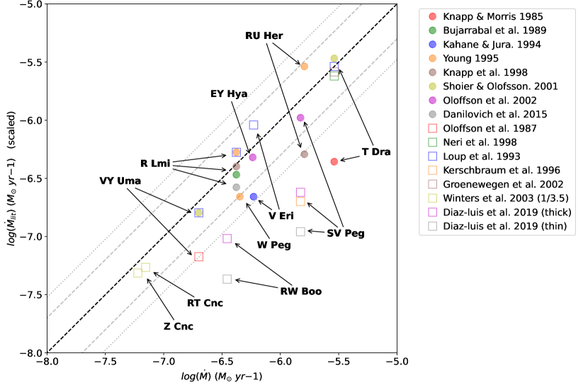
Figure 12: Comparison between mass-loss rates scaled values from the literature ($\dot{M}$_lit) and $\dot{M}$  obtained in this work fitted with $\mbox{$R_{\rm s}$}=\mbox{$R_{\rm CO}$}/2.5$. The solid line indicates equality, the dashed lines relationships 1/2 and 2, and the dotted lines relationships 1/3 and 3. Filled circles and empty squares indicate previous studies with radiative transfer models and with empirical laws, respectively.

Figure 12 shows the properly scaled $\dot{M}$-to-$\dot{M}$_lit comparison. Overall, the obtained values of the mass-loss are in good agreement (within a factor 3) with those from the literature, specially those obtained from radiative transfer models and using more than one CO transitions, which are expected to provide the most reliable and accurate values. In a few cases, larger discrepancies are observed, which can be attributed to different factors, namely, marginal line(s) detection, calibration uncertainties, etc, which are discussed in some detail below. We can safely conclude that uncertainties in our mass-loss estimates are not lower than a factor $\approx$3, but probably not significantly larger considering the moderate scatter of points in Fig. 12. This is comparable to uncertainties in most previous CO-based studies using different methods, even using radiative transfer models as shown in Fig. 12. The largest source of uncertainty in our estimate, and in many previous works, probably lies on the lack of a precise value of the characteristic radius of the CO envelope ($R_{\rm s}$), which can only be improved by carrying out interferometric CO emission mapping.

In the following paragraphs we list in some detail previous CO detections and mass-loss rates estimates for individual targets, together with a brief description of some of their properties:

EY Hya is a 180 day period O-rich semi-regular (SRa) variable. There are previous ¹²CO ($J$=2–1)  and ¹²CO ($J$=3–2)  detections and a CO-based mass-loss rate estimation.

Olofsson et al. (2002) used the ¹²CO ($J$=2–1)  and ¹²CO ($J$=3–2)  detections presented in Kerschbaum & Olofsson (1999) to evaluate the mass-loss rate using a radiative transfer code. The value obtained is $\dot{M}$=2.5$\times 10^{\rm-7}$ $M_{\odot}$ yr^-1 ($D$=300 pc, $V_{\rm exp}$=11 km s^-1, and $X_{\rm CO}$=2$\times 10^{\rm-4}$), which scaled to the values of $D$, $V_{\rm exp}$ and $X_{\rm CO}$values used by us (tables 1 and 5) is $\dot{M}$=4.8$\times 10^{\rm-7}$ $M_{\odot}$ yr^-1.

R Lmi is a 370 day period O-rich Mira variable. There are previous ¹²CO ($J$=2–1) , ¹²CO ($J$=3–2)  and ¹²CO ($J$=4–3)  detections and CO-based mass-loss rate estimations.

Bujarrabal et al. (1989) reported a ¹²CO ($J$=1–0)  detection. They used a Large Velocity Gradient model to fit the ¹²CO ($J$=3–2) and SiO($J$=2-1) line profiles and evaluate the mass-loss rate. The value obtained is $\dot{M}$=5ex-7 $M_{\odot}$ yr^-1 ($D$=350 pc, $V_{\rm exp}$=6.4 km s^-1, and $X_{\rm CO}$=2$\times 10^{\rm-4}$), which scaled to the values of $D$, $V_{\rm exp}$ and $X_{\rm CO}$values used by us (tables 1 and 5) is $\dot{M}$=3.4$\times 10^{\rm-7}$ $M_{\odot}$ yr^-1.

Loup et al. (1993) used the ¹²CO ($J$=1–0)detection reported by Bujarrabal et al. (1986) to evaluate the mass-loss rate using the formulation of Knapp & Morris (1985). The value obtained is $\dot{M}$=2.8$\times 10^{\rm-7}$ $M_{\odot}$ yr^-1 ($D$=330 pc, $V_{\rm exp}$=7.0 km s^-1, and $X_{\rm CO}$=5$\times 10^{\rm-4}$), which scaled to the values of $D$, $V_{\rm exp}$ and $X_{\rm CO}$values used by us (tables 1 and 5) is $\dot{M}$=5.3$\times 10^{\rm-7}$ $M_{\odot}$ yr^-1.

Young (1995) reported a ¹²CO ($J$=3–2)  and ¹²CO ($J$=4–3)  detections. They used a Large Velocity Gradient model to fit the peak temperature of the ¹²CO ($J$=3–2)  line profile and evaluate the mass-loss rate. The value obtained is $\dot{M}$=1.6$\times 10^{\rm-7}$ $M_{\odot}$ yr^-1 ($D$=260 pc, $V_{\rm exp}$=8.7 km s^-1, and $X_{\rm CO}$=3$\times 10^{\rm-4}$), which scaled to the values of $D$, $V_{\rm exp}$ and $X_{\rm CO}$values used by us (tables 1 and 5) is $\dot{M}$=5.3$\times 10^{\rm-7}$ $M_{\odot}$ yr^-1.

Knapp et al. (1998) reported a ¹²CO ($J$=2–1)  detection. These authors evaluate the mass-loss rate using a radiative transfer model. The value obtained is $\dot{M}$=1.6$\times 10^{\rm-7}$ $M_{\odot}$ yr^-1 ($D$=270 pc, $V_{\rm exp}$=7.8 km s^-1, and $X_{\rm CO}$=5$\times 10^{\rm-4}$), which scaled to the values of $D$, $V_{\rm exp}$ and $X_{\rm CO}$values used by us (tables 1 and 5) is $\dot{M}$=4.0$\times 10^{\rm-7}$ $M_{\odot}$ yr^-1.

Danilovich et al. (2015) used a detailed radiative transfer model to fit the ¹²CO ($J$=2–1)  and ¹²CO ($J$=3–2)line profiles and evaluate the mass-loss rate. The value obtained is $\dot{M}$=2.6$\times 10^{\rm-7}$ $M_{\odot}$ yr^-1 ($D$=330 pc, $V_{\rm exp}$=7.5 km s^-1, and $X_{\rm CO}$=3$\times 10^{\rm-4}$), which scaled to the values of $D$, $V_{\rm exp}$ and $X_{\rm CO}$values used by us (tables 1 and 5) is $\dot{M}$=2.7$\times 10^{\rm-7}$ $M_{\odot}$ yr^-1.

RT Cnc is a 90 day period O-rich semi-regular (SRb) variable. There is a previous ¹²CO ($J$=2–1)  detection and a CO-based mass-loss rate estimation.

Winters et al. (2003) reported a ¹²CO ($J$=2–1)  detection, which they use to evaluate both the mass-loss rate using the formulation of Loup et al. (1993) (first introduced by Knapp & Morris 1985). The value obtained is $\dot{M}$=4.4$\times 10^{\rm-7}$ $M_{\odot}$ yr^-1 ($D$=340 pc, $V_{\rm exp}$=12 km s^-1, and $X_{\rm CO}$=2$\times 10^{\rm-4}$), which scaled to the values of $D$, $V_{\rm exp}$ and $X_{\rm CO}$values used by us (tables 1 and 5) is $\dot{M}$=1.9$\times 10^{\rm-7}$ $M_{\odot}$ yr^-1. Winters et al. (2003) note that their values for $\dot{M}$  are systematically larger by a factor 3.5 than those obtained by Olofsson et al. (2002) for a number of objects in common in both works. Considering a correction by a factor 3.5, the value of $\dot{M}$ derived Winters et al. (2003) becomes 5.4$\times 10^{\rm-8}$ $M_{\odot}$ yr^-1.

RU Her is a 480 day period Mira (M) variable. There are previous ¹²CO ($J$=2–1) , ¹²CO ($J$=3–2)  and ¹²CO ($J$=4–3)  detections and CO-based mass-loss rate estimations.

Young (1995) reported a ¹²CO ($J$=3–2)  and ¹²CO ($J$=4–3)  detections.They used a Large Velocity Gradient model to fit the peak temperature of the ¹²CO ($J$=3–2)  line profile and evaluate the mass-loss rate. The value obtained is $\dot{M}$=7.5$\times 10^{\rm-7}$ $M_{\odot}$ yr^-1 ($D$=410 pc, $V_{\rm exp}$=8.9 km s^-1, and $X_{\rm CO}$=3$\times 10^{\rm-4}$), which scaled to the values of $D$, $V_{\rm exp}$ and $X_{\rm CO}$values used by us (tables 1 and 5) is $\dot{M}$=2.9$\times 10^{\rm-6}$ $M_{\odot}$ yr^-1.

Knapp et al. (1998) reported a ¹²CO ($J$=2–1)  detection which they use to evaluate both the mass-loss rate using a radiative transfer model. The value obtained is $\dot{M}$=3.2$\times 10^{\rm-7}$ $M_{\odot}$ yr^-1 ($D$=400 pc, $V_{\rm exp}$=9.4 km s^-1, and $X_{\rm CO}$=5$\times 10^{\rm-4}$), which scaled to the values of $D$, $V_{\rm exp}$ and $X_{\rm CO}$values used by us (tables 1 and 5) is $\dot{M}$=5.1$\times 10^{\rm-7}$ $M_{\odot}$ yr^-1.

RW Boo is a 209 day period O-rich semi-regular (SRb) variable. There are previous ¹²CO ($J$=1–0)  and ¹²CO ($J$=2–1)  detections and a CO-based mass-loss rate estimation.

Díaz-Luis et al. (2019) reported ¹²CO ($J$=1–0)  and ¹²CO ($J$=2–1)  detections and estimated the mass-loss rate using the formulation based on that presented in Knapp & Morris (1985), in the case of optically thick envelope and in the case of optically thin. The values obtained are $\mbox{$\dot{M}$}_{thick}$=9.9$\times 10^{\rm-8}$ $M_{\odot}$ yr^-1 and $\mbox{$\dot{M}$}_{thin}$=4.4$\times 10^{\rm-8}$ $M_{\odot}$ yr^-1 ($D$=307 pc, $V_{\rm exp}$=17.29 km s^-1, and $X_{\rm CO}$=3$\times 10^{\rm-4}$), which scaled to the values of $D$, $V_{\rm exp}$ and $X_{\rm CO}$values used by us (tables 1 and 5) is $\mbox{$\dot{M}$}_{thick}$=9.6$\times 10^{\rm-8}$ $M_{\odot}$ yr^-1and $\mbox{$\dot{M}$}_{thin}$=4.3$\times 10^{\rm-8}$ $M_{\odot}$ yr^-1.

SV Peg is a 145 day period O-rich semi-regular (SRb) variable. There are previous¹²CO ($J$=1–0), ¹²CO ($J$=2–1)  and ¹²CO ($J$=3–2)  detections and CO-based mass-loss rate estimations.

Kerschbaum et al. (1996) reported ¹²CO ($J$=1–0)  and ¹²CO ($J$=2–1)  detections which they use to evaluate both the mass-loss rate using the formulation of Kastner (1992). The value obtained is $\dot{M}$=1.0$\times 10^{\rm-7}$ $M_{\odot}$ yr^-1 ($D$=230 pc, $V_{\rm exp}$=10.6 km s^-1, and $X_{\rm CO}$=2$\times 10^{\rm-4}$), which scaled to the values of $D$, $V_{\rm exp}$ and $X_{\rm CO}$values used by us (tables 1 and 5) is $\dot{M}$=2.0$\times 10^{\rm-7}$ $M_{\odot}$ yr^-1.

Olofsson et al. (2002) used the ¹²CO ($J$=1–0) , ¹²CO ($J$=2–1)  and ¹²CO ($J$=3–2)  detections presented in Kerschbaum & Olofsson (1999) to evaluate the mass-loss rate using a radiative transfer code. The value obtained is $\dot{M}$=3.0$\times 10^{\rm-7}$ $M_{\odot}$ yr^-1 ($D$=190 pc, $V_{\rm exp}$=7.5 km s^-1, and $X_{\rm CO}$=2$\times 10^{\rm-4}$), which scaled to the values of $D$, $V_{\rm exp}$ and $X_{\rm CO}$values used by us (tables 1 and 5) is $\dot{M}$=1.1$\times 10^{\rm-6}$ $M_{\odot}$ yr^-1.

Díaz-Luis et al. (2019) reported ¹²CO ($J$=1–0)  and ¹²CO ($J$=2–1)  detections and estimated the mass-loss rate using the formulation based on that presented in Knapp & Morris (1985), in the case of optically thick envelope and in the case of optically thin. The values obtained are $\mbox{$\dot{M}$}_{thick}$=1.1$\times 10^{\rm-6}$ $M_{\odot}$ yr^-1 and $\mbox{$\dot{M}$}_{thin}$=4.8$\times 10^{\rm-7}$ $M_{\odot}$ yr^-1 ($D$=890 pc, $V_{\rm exp}$=9.07 km s^-1, and $X_{\rm CO}$=3$\times 10^{\rm-4}$), which scaled to the values of $D$, $V_{\rm exp}$ and $X_{\rm CO}$values used by us (tables 1 and 5) is $\mbox{$\dot{M}$}_{thick}$=2.4$\times 10^{\rm-7}$ $M_{\odot}$ yr^-1and $\mbox{$\dot{M}$}_{thin}$=1.1$\times 10^{\rm-7}$ $M_{\odot}$ yr^-1.

T Dra is a 420 day period C-rich Mira variable. There are previous ¹²CO ($J$=1–0)  and ¹²CO ($J$=2–1)  detections and CO-based mass-loss rate estimations.

Knapp & Morris (1985) reported a tentative ¹²CO ($J$=1–0)  detection with low S/N. They used a radiative transfer model to fit the ¹²CO ($J$=1–0)  line profile and evaluate the mass-loss rate. The value obtained is $\dot{M}$=1.3 $\times 10^{\rm-6}$ $M_{\odot}$ yr^-1 ($D$=525 pc, $V_{\rm exp}$=14.0 km s^-1, and $X_{\rm CO}$=8$\times 10^{\rm-4}$), which scaled to the values of $D$, $V_{\rm exp}$ and $X_{\rm CO}$values used by us (tables 1 and 5) is $\dot{M}$=4.4$\times 10^{\rm-7}$ $M_{\odot}$ yr^-1. The mass-loss rate discrepancy (with respect to our value of $\dot{M}$ (by a factor $\sim$7) in this case can be mainly attributed to the marginal detection of the ¹²CO ($J$=1–0) line and the lack of a constraint for the excitation temperature in the work by Knapp & Morris (1985).

Loup et al. (1993) used the ¹²CO ($J$=1–0) detection reported by Knapp & Morris (1985); Margulis et al. (1990); Nyman et al. (1992) to evaluate the mass-loss rate using the formulation of Knapp & Morris (1985). The value obtained is $\dot{M}$=2.2$\times 10^{\rm-6}$ $M_{\odot}$ yr^-1 ($D$=910 pc, $V_{\rm exp}$=13.1 km s^-1, and $X_{\rm CO}$=1$\times 10^{\rm-3}$), which scaled to the values of $D$, $V_{\rm exp}$ and $X_{\rm CO}$values used by us (tables 1 and 5) is $\dot{M}$=2.9$\times 10^{\rm-6}$ $M_{\odot}$ yr^-1.

Neri et al. (1998) reported ¹²CO ($J$=1–0)  and ¹²CO ($J$=2–1)  interferometric maps obtined with the IRAM Plateau de Bure Interferometer (PdBI) as well as single-dish IRAM-30 m spectra, which they use to evaluate both the mass-loss rate using the formulation of Loup et al. (1993) (first introduced by Knapp & Morris 1985). The value obtained is $\dot{M}$=2.9$\times 10^{\rm-6}$ $M_{\odot}$ yr^-1 ($D$=910 pc, $V_{\rm exp}$=14.3 km s^-1, and $X_{\rm CO}$=1$\times 10^{\rm-3}$), which scaled to the values of $D$, $V_{\rm exp}$ and $X_{\rm CO}$values used by us (tables 1 and 5) is $\dot{M}$=2.4$\times 10^{\rm-6}$ $M_{\odot}$ yr^-1. They also estimated the source radius directly from the interferometric maps of $\simeq$8.7″, which is comparable to, but slightly larger than, the $R_{\rm CO}$/2.5 approximation used by us resulting in $\theta_{\rm s}$$\simeq$4.8″.

Schöier & Olofsson (2001) used a detailed radiative transfer analysis in combination with an energy balance equation for the gas to model the ¹²CO ($J$=1–0)  and ¹²CO ($J$=2–1)  detections reported by Olofsson et al. (1993) and the ¹²CO ($J$=1–0) detection reported by Neri et al. (1998). The value obtained is $\dot{M}$=1.2$\times 10^{\rm-6}$ $M_{\odot}$ yr^-1 ($D$=610 pc, $V_{\rm exp}$=13.5 km s^-1, and $X_{\rm CO}$=1$\times 10^{\rm-3}$), which scaled to the values of $D$, $V_{\rm exp}$ and $X_{\rm CO}$values used by us (tables 1 and 5) is $\dot{M}$=3.4$\times 10^{\rm-6}$ $M_{\odot}$ yr^-1, which is in very good agreement with our estimate $\dot{M}$=[1.6-2.9]$\times 10^{\rm-6}$ $M_{\odot}$ yr^-1 (adopting Re=$R_{\rm CO}$ and Re=$R_{\rm CO}$/2.5, respectively).

Groenewegen et al. (2002b) used the ¹²CO ($J$=2–1)  detection reported by Groenewegen et al. (2002a) to evaluate the mass-loss rate using the formulation of Olofsson et al. (1993). The value obtained is $\dot{M}$=2.4$\times 10^{\rm-6}$ $M_{\odot}$ yr^-1 ($D$=860 pc, $V_{\rm exp}$=16.8 km s^-1, and $X_{\rm CO}$=8$\times 10^{\rm-4}$), which scaled to the values of $D$, $V_{\rm exp}$ and $X_{\rm CO}$ values used by us (tables 1 and 5) is $\dot{M}$=2.6$\times 10^{\rm-6}$ $M_{\odot}$ yr^-1.

V Eri is a 100 day period semi-irregular (SRC) variable. There are previous ¹²CO ($J$=1–0)  and ¹²CO ($J$=2–1)  detections and CO-based mass-loss rate estimations.

Loup et al. (1993) used the ¹²CO ($J$=2–1)  detection reported by Zuckerman & Dyck (1986) to evaluate the mass-loss rate using the formulation of Knapp & Morris (1985). The value obtained is $\dot{M}$=1.1$\times 10^{\rm-6}$ $M_{\odot}$ yr^-1 ($D$=460 pc, $V_{\rm exp}$=13 km s^-1, and $X_{\rm CO}$=5$\times 10^{\rm-4}$), which scaled to the values of $D$, $V_{\rm exp}$ and $X_{\rm CO}$values used by us (tables 1 and 5) is $\dot{M}$=9.1$\times 10^{\rm-7}$ $M_{\odot}$ yr^-1.

Kahane & Jura (1994) reported ¹²CO ($J$=1–0)  and ¹²CO ($J$=2–1)  detections. They used a Large Velocity Gradient model to fit both line profiles and evaluate the mass-loss rate. The value obtained is $\dot{M}$=2.9ex-7 $M_{\odot}$ yr^-1 ($D$=250 pc, $V_{\rm exp}$=11.0 km s^-1, and $X_{\rm CO}$=2$\times 10^{\rm-4}$), which scaled to the values of $D$, $V_{\rm exp}$ and $X_{\rm CO}$values used by us (tables 1 and 5) is $\dot{M}$=2.2$\times 10^{\rm-7}$ $M_{\odot}$ yr^-1.

VY Uma is a C-rich irregular variable. There are previous ¹²CO ($J$=1–0)  and ¹²CO ($J$=2–1)  detections and CO-based mass-loss rate estimations.

Olofsson et al. (1987) reported a ¹²CO ($J$=1–0)  detection which they use to evaluate both the mass-loss rate using the formulation of Knapp & Morris (1985). The value obtained is $\dot{M}$=1.3$\times 10^{\rm-7}$ $M_{\odot}$ yr^-1 ($D$=520 pc, $V_{\rm exp}$=8.4 km s^-1, and $X_{\rm CO}$=8$\times 10^{\rm-4}$), which scaled to the values of $D$, $V_{\rm exp}$ and $X_{\rm CO}$values used by us (tables 1 and 5) is $\dot{M}$=6.7$\times 10^{\rm-8}$ $M_{\odot}$ yr^-1.

Loup et al. (1993) used the ¹²CO ($J$=1–0)  detection reported by Olofsson et al. (1987) to evaluate the mass-loss rate using the formulation of Knapp & Morris (1985). The value obtained is $\dot{M}$=4.8$\times 10^{\rm-7}$ $M_{\odot}$ yr^-1 ($D$=750 pc, $V_{\rm exp}$=7.9 km s^-1, and $X_{\rm CO}$=1$\times 10^{\rm-3}$), which scaled to the values of $D$, $V_{\rm exp}$ and $X_{\rm CO}$values used by us (tables 1 and 5) is $\dot{M}$=1.6$\times 10^{\rm-7}$ $M_{\odot}$ yr^-1.

Schöier & Olofsson (2001) used a detailed radiative transfer analysis in combination with an energy balance equation for the gas to model the ¹²CO ($J$=1–0)  and ¹²CO ($J$=2–1)  detections reported by Olofsson et al. (1993). The value obtained is $\dot{M}$=7$\times 10^{\rm-8}$ $M_{\odot}$ yr^-1 ($D$=330 pc, $V_{\rm exp}$=6 km s^-1, and $X_{\rm CO}$=1$\times 10^{\rm-3}$), which scaled to the values of $D$, $V_{\rm exp}$ and $X_{\rm CO}$values used by us (tables 1 and 5) is $\dot{M}$=1.6$\times 10^{\rm-7}$ $M_{\odot}$ yr^-1.

W Peg is a 350 day period Mira (M) variable. There is a previous ¹²CO ($J$=3–2)  detection and a CO-based mass-loss rate estimation.

Young (1995) reported a ¹²CO ($J$=3–2)  detection and used a Large Velocity Gradient model to fit the peak temperature of the ¹²CO ($J$=3–2)  line profile and evaluate the mass-loss rate. The value obtained is $\dot{M}$=9.8$\times 10^{\rm-8}$ $M_{\odot}$ yr^-1 ($D$=270 pc, $V_{\rm exp}$=7.7 km s^-1, and $X_{\rm CO}$=3$\times 10^{\rm-4}$), which scaled to the values of $D$, $V_{\rm exp}$ and $X_{\rm CO}$values used by us (Tables 1 and 5) is $\dot{M}$=2.2$\times 10^{\rm-7}$ $M_{\odot}$ yr^-1.

Z Cnc is a 95 day period O-rich semi-regular (SRb) variable. There is a previous ¹²CO ($J$=2–1)  detection and a CO-based mass-loss rate estimation.

Winters et al. (2003) reported a ¹²CO ($J$=2–1)  detection, which they use to evaluate both the mass-loss rate using the formulation of Loup et al. (1993) (first introduced by Knapp & Morris 1985). The value obtained is $\dot{M}$=3$\times 10^{\rm-7}$ $M_{\odot}$ yr^-1 ($D$=389 pc, $V_{\rm exp}$=8 km s^-1, and $X_{\rm CO}$=2$\times 10^{\rm-4}$), which scaled to the values of $D$, $V_{\rm exp}$ and $X_{\rm CO}$values used by us (Tables 1 and 5) is $\dot{M}$=1.8$\times 10^{\rm-7}$ $M_{\odot}$ yr^-1. Winters et al. (2003) note that their values for $\dot{M}$  are systematically larger by a factor 3.5 than those obtained by Olofsson et al. (2002) for a number of objects in common in both works. Considering a correction by a factor 3.5, the value of $\dot{M}$ derived Winters et al. (2003) becomes 5.1$\times 10^{\rm-8}$ $M_{\odot}$ yr^-1.

Appendix E Population diagrams of CO

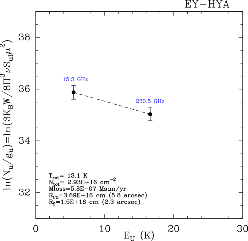
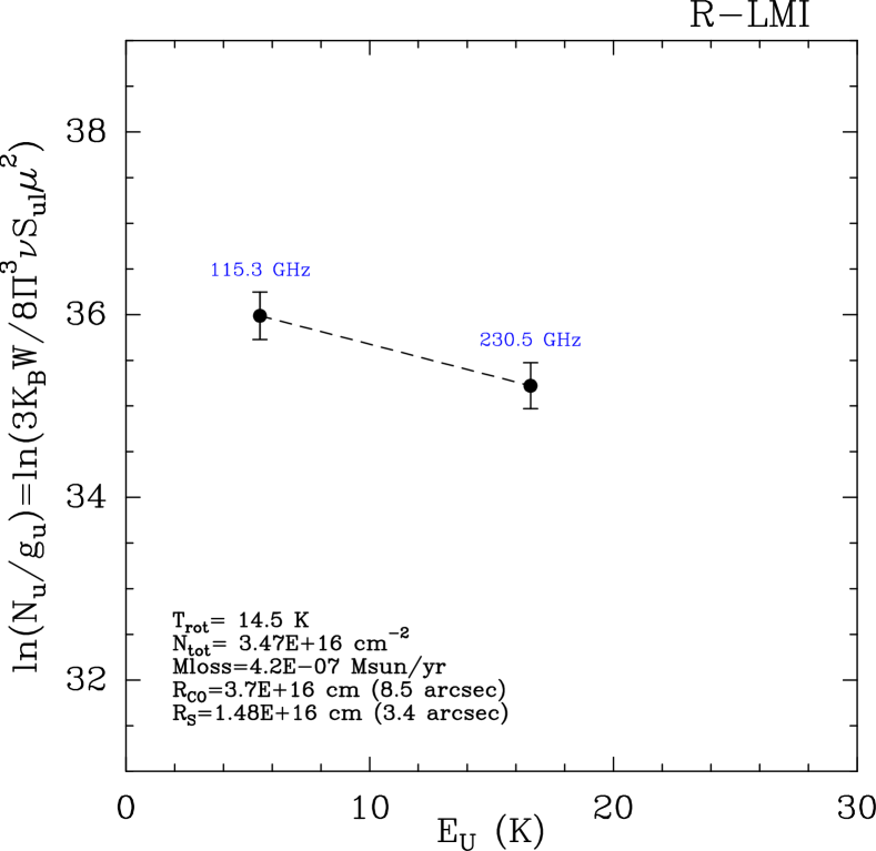
Figure 13: Opacity-corrected population diagrams for uvAGB stars with CO detections (see Appendix E). Upper limits (3$\sigma$) for ¹²CO ($J$=1–0) non-detections are indicated by triangles. Values of the main envelope parameters deduced from the fits (dashed line) are indicated in the bottom left corner of the boxes.

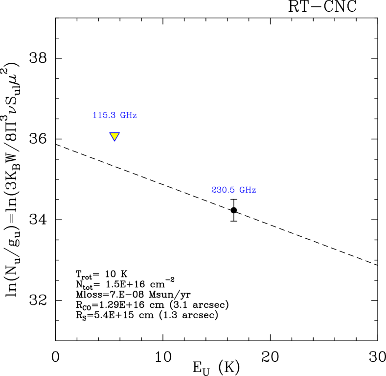
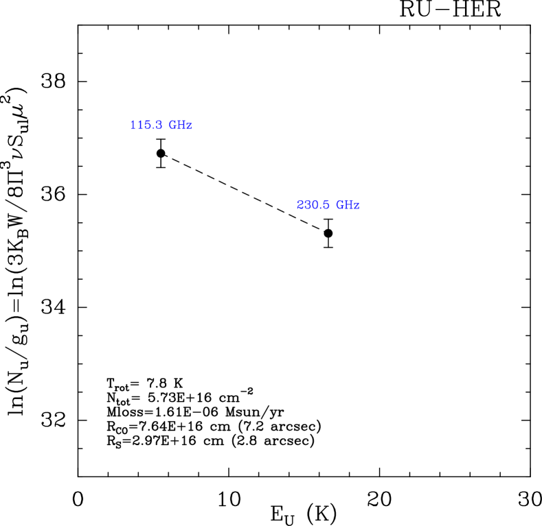
Fig. 13 continued.

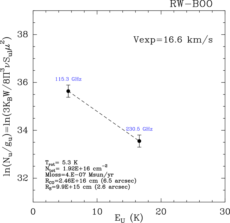
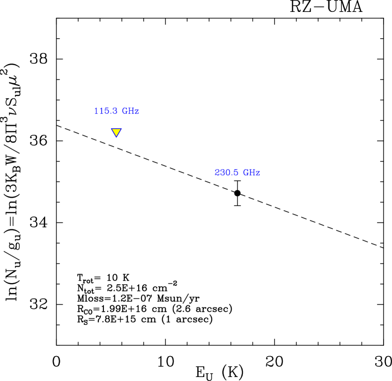
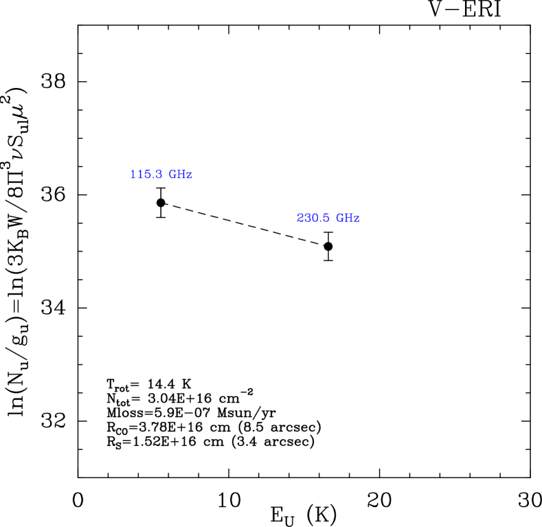
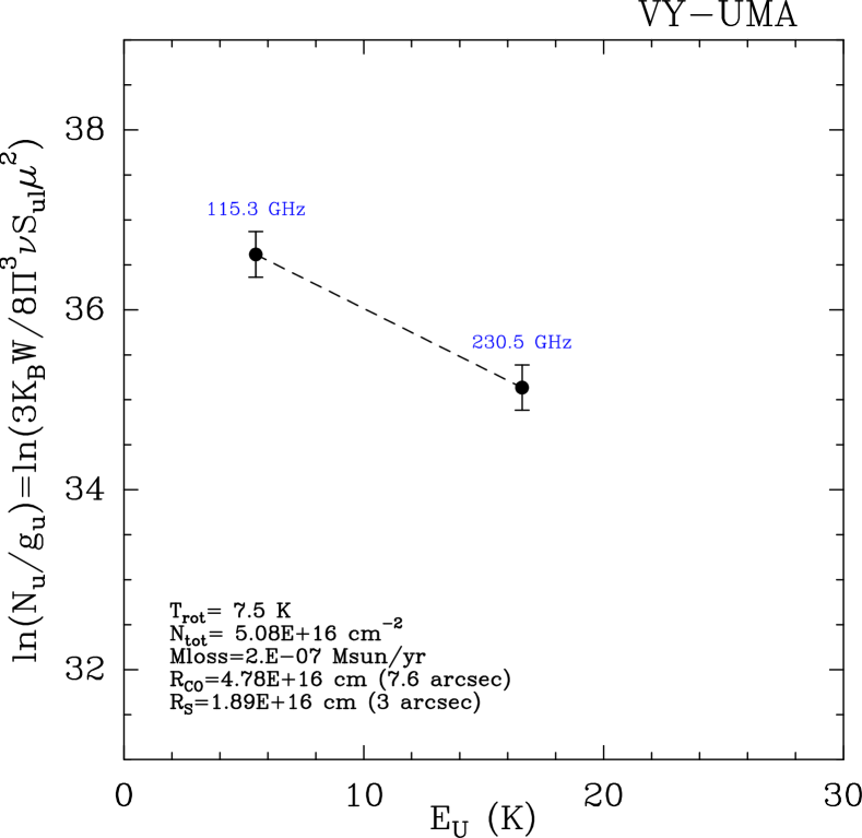
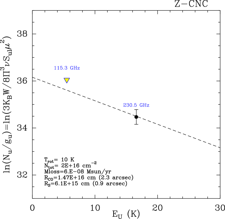
Fig. 13 continued.

Fig. 13 continued.

Fig. 13 continued.