Testing General Relativity with NuSTAR data of Galactic Black Holes : \Romannum2
Abstract
General Relativity predicts the spacetime metric around an astrophysical black hole to be described by Kerr solution which is a massive rotating black hole without any residual charge. In a previous paper, we analyzed the NuSTAR observations of six X-ray binaries to obtain constraints on deformation parameter using a state-of-the-art relativistic model. In this work, we continue analyzing NuSTAR observations of four more X-ray Binaries; two of which are X-ray Transients very close to the supermassive black hole at the center of our galaxy. The other two sources have complicated absorption which is accounted by time-resolved and flux-resolved spectroscopy. The constraints obtained are consistent with the Kerr hypothesis and are comparable with those obtained in previous studies and those from gravitational events.
1. Introduction
In 1915, Albert Einstein proposed the theory of General Relativity (GR) (Einstein, 1916) and after four years, it successfully passed the test conducted by Eddington during the total Solar eclipse. After this experiment in a weak-field regime, this theory has passed other such tests in the Solar system and in observations of binary Pulsars (Will, 2014). After passing successfully in the weak-field limit, there has been an increased interest in the scientific community to test this theory in a strong-field regime. Thanks to technological advancements, the last decade has seen an immense improvement in testing this theory, and now, we can test the predictions of GR with X-ray data (e.g., Cao et al., 2018; Tripathi et al., 2019, 2020b, 2021a), Very Long Baseline Interferometry (VLBI) (e.g., Psaltis et al., 2020) and gravitational wave observations (e.g., Abbott et al., 2016; Yunes et al., 2016; Abbott et al., 2019).
Black holes are the 4-dimensional solutions of Einstein’s equations. The uncharged spinning black holes are given by the Kerr solution (Kerr, 1963) which describes the spacetime metric around the astrophysical black holes. This is the direct consequence of “no-hair” theorems where the black hole is simply quantified by three quantities; mass, spin, and charge. It is also found that deviations caused by non-vanishing electric charge, nearby stars, and the accretion disk are negligible (see, e.g., Bambi et al., 2014; Bambi, 2018). There are several scenarios where the macroscopic deviations from the Kerr solution are possible (e.g., Giddings, 2017; Herdeiro & Radu, 2014). These scenarios include the models with macroscopic quantum gravity effects or the models with the presence of exotic matter fields. It is also possible that the classical extension of GR exists and also the GR is not the correct theory of gravity (e.g., Kleihaus et al., 2011). Thus, testing the Kerr hypothesis around the black holes is a means by which GR in a strong-field regime can be tested.
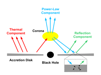
X-ray Reflection Spectroscopy is one of the most suitable methods to determine the properties of black holes by studying the reflection spectrum emitted by the accretion disk around it (Brenneman & Reynolds, 2006). The schematic representation of an astrophysical black hole system is shown in Fig. 1. For stellar-mass black holes, the temperature of the accretion disk lies in the soft X-rays (0.1-1.0 keV). A part of the thermal component interacts with the electrons via inverse Compton scattering present in the corona which is a hot ( 100 keV) and optically thin medium above the black hole. This inverse Compton scattering generates a power-law component with a cutoff energy of about 300 keV. A part of this power law component illuminates the disk and produces the reflection spectrum constituting various emission and absorption features. The most prominent reflection signatures are the Iron K line around 6 keV and the Compton hump around 20 keV(Ross & Fabian, 2005; García & Kallman, 2010). The reflection spectrum at any point on the disk in the rest frame of the gas is determined by atomic physics where the atomic transitions of ionized ions are treated in detail. The photons travel in the strong gravitational field present around black holes and are affected by relativistic effects such as light bending, Doppler broadening, gravitational redshift, etc., before reaching the observer. In the presence of high-resolution data (so that the reflection features can be resolved) and the correct astrophysical effects (to account for the relativistic effects and emission lines), we can thus probe the regions that are very close to the black hole (Reynolds, 2019). We can also measure the reflection spectrum accurately which will be helpful to determine the spacetime metric around the black hole and thus test the Kerr hypothesis around astrophysical black holes.
Our group has developed a model relxill_nk (Bambi et al., 2017; Abdikamalov et al., 2019) to test the Kerr hypothesis using X-ray Reflection Spectroscopy around black holes. relxill_nk is the extension of relxill (Dauser et al., 2013; García et al., 2014) to non-Kerr metrics such as Johannsen metric, KRZ metric, etc. The reflection spectrum at an emission point in the rest frame of the gas in the accretion disk is modified by the relativistic convolution model for a background metric. The deviations from the Kerr solutions in the background metric are quantified by “deformation parameters” which vanishes for the Kerr solution. Comparison of the X-ray observations of black holes against the theoretical modeling of relxill_nk measures the deformation parameters and thus tests the Kerr hypothesis in a strong-field regime.
In the past five years, we employed relxill_nk to constrain the deformation parameters using X-ray observations of various X-ray binaries and supermassive black holes (Bambi, 2017; Bambi et al., 2017, 2021; Abdikamalov et al., 2019, 2020). The most stringent constraint obtained is for the simultaneous Swift and NuSTAR observation of GX 339-4 (Tripathi et al., 2021). All measurements of deformation parameters are consistent with the Kerr hypothesis.
In Tripathi et al. (2021a), we applied relxill_nk to analyze the reflection spectrum of six X-ray binaries observed by NuSTAR observations. We obtained the most robust constraints on the Kerr hypothesis available to date. The constraints of these X-ray binaries are comparable to those obtained from gravitational waves and other electromagnetic techniques. Motivated by our results, we selected the complicated sources from the list of all published spin measurements using NuSTAR. For these observations, the inner edge of the accretion is very close to the black hole which is considered favorable for obtaining tight constraints on the deformation parameters. Also, these sources are found to have high spin which is also an essential requirement for getting stringent constraints on the deviations from the Kerr hypothesis.
This manuscript is organized as follows. In Section 2, we will briefly describe the selection of sources and observations. The spectral analysis for each source is presented in Section 3. In Section 4, we discuss and summarise the results. Throughout the paper, we adopt the convention (-+++) and =c=1.
2. Selection of the sources and data reduction
We started with the list of all published spin measurements done by NuSTAR (Harrison et al., 2013). NuSTAR is considered to be currently the best X-ray mission to study the reflection features originating in the innermost regions of black holes where the effects of gravity are immense. The main advantage of NuSTAR is the coverage of a wide energy range of 3-79 keV which includes two of the most prominent reflection features; Iron line and Compton hump. Besides, pile-up is absent which is usually the dominant effect for the bright sources.
In (Tripathi et al., 2021a), we selected six sources from the list of fourteen objects given in Tab. 1 which has a reflection spectrum minimally affected by absorption, dust scattering, and have accretion disk extends up to ISCO. These six sources are GX 339-4, Swift J168.2—4242, 4U 1630–472, GRS 1739–278, GS 1354-645, and EXO 1846–031. In this paper, we analyzed the observations for which the variability and absorptions could be modeled by applying advanced spectroscopic and reduction methods like flux-resolved, flare-resolved, and time-resolved spectroscopy, etc. In this work, we analyze the NuSTAR observations of four sources: Swift J174540.7–290015, Swift J174540.2–290037, MAXI J1631–479, and V404 Cygni.
| Source | Mission(s) | State | Reference | |
|---|---|---|---|---|
| 4U 1630–472 | NuSTAR | Intermediate | King et al. (2014) | |
| Cyg X-1 | NuSTAR+Suzaku | Soft | Tomsick et al. (2014) | |
| NuSTAR+Suzaku | Hard | Parker et al. (2015) | ||
| NuSTAR | Soft | Walton et al. (2016) | ||
| EXO 1846–031 | NuSTAR | Hard intermediate | Draghis et al. (2020) | |
| GRS 1716–249 | NuSTAR+Swift | Hard Intermediate | Tao et al. (2019) | |
| GRS 1739–278 | NuSTAR | Low/Hard | Miller et al. (2015) | |
| GRS 1915+105 | NuSTAR | Low/Hard | Miller et al. (2013) | |
| GS 1354–645 | NuSTAR | Hard | El-Batal et al. (2016) | |
| GX 339–4 | NuSTAR+Swift | Very High | Parker et al. (2016) | |
| MAXI J1535–571 | NuSTAR | Hard | Xu et al. (2018a) | |
| MAXI J1631–479 | NuSTAR | Soft | Xu et al. (2020) | |
| Swift J1658.2–4242 | NuSTAR+Swift | Hard | Xu et al. (2018b) | |
| Swift J174540.2–290037 | Chandra+NuSTAR | Hard | Mori et al. (2019) | |
| Swift J174540.7–290015 | Chandra+NuSTAR | Soft | Mori et al. (2019) | |
| V404 Cyg | NuSTAR | Hard | Walton et al. (2017) |
2.1. Data reduction
| Source | Observation ID | Observation Date |
|---|---|---|
| SWIFT J174540.7-290015 | 90101022002 | 2016 February 22 |
| SWIFT J174540.2-290037 | 90201026002 | 2016 June 9 |
| MAXI J1631-479 | 90501301001 | 2019 Jan 17 |
| V404Cygni | 90102007002/3 | 2015 July 11 |
Tab. 2 presents the details of the observations of four sources analyzed in this work. The unfiltered events from the FPMA and FPMB instruments of NuSTAR are converted into cleaned events using the latest calibration files and the latest version of NuSTAR data analysis software (NuSTARDAS) v2.0.0 which is distributed as a part of HEASOFT package. We select the source region with a center at the source such that around 90 percent of source photons will be captured. The background region is selected as far as possible from the source on the same detector so that the effect of the source is not significant. The end products i.e., the spectrum and light curve, are generated using nupipeline routine of NuSTARDAS. The cross-calibration constant between FPMA is kept frozen at 1.0 and thawed for FPMB of each observation. We will discuss the details of data reduction for each source separately.
3. Spectral analysis
Various models are employed to explain the different emissions from the black hole systems. Now, we will discuss these models.
Tbabs (Wilms et al., 2000) account for X-ray absorption in the Inter-Stellar Medium (ISM). Here, the free parameters are hydrogen equivalent column density. The abundance of other elements is assumed to be the default for this work. In some sources with heavy absorption, we use Tbnew (Wilms et al., 2000) which allows us to change the column density of other elements and takes into account the depletion of elements. For simplicity, we kept all parameters but the column density of Hydrogen frozen.
The accretion disk around the black hole is assumed to be optically thick and geometrically thin. The temperature of the disk lies in the soft X-ray band ( 1 keV) and emits blackbody radiation. The whole accretion disk emits a multi-temperature blackbody-like spectrum. This spectrum is described by the model diskbb (Mitsuda et al., 1984) in XSPEC. The parameters are the inner temperature of the disk (in keV) and normalization. These thermal photons interact with the electrons present in the corona via Compton inverse-scattering. Corona is believed to be a hotter cloud of gas with a temperature of around 100 keV situated above the black hole and accretion disk. This interaction leads to the generation of a continuum with exponential energy cut-off. The power-law photon continuum is described by the additive model powerlaw. The parameters are photon index , cut-off energy , and normalization. Another model compTT (Titarchuk, 1994) describes the Comptonized continuum and also includes relativistic effects.
A part of the continuum produced in the corona reaches the observer and another part illuminates the disk producing various emission lines together referred to as the reflection spectrum. The most prominent reflection signatures are iron K emission around 6-7 keV and the Compton hump around 20 keV. xillver (García & Kallman, 2010; García et al., 2014) describes the reflection spectrum in the rest frame of the gas which is not significantly affected by the strong gravity of a black hole. The parameters of this model are the photon index of the incident continuum , ionization of the disk log, iron abundance in Solar units , and reflection fraction . The reflection spectrum generated in the inner regions of a black hole is affected by its strong gravity. relxill_nk describes the relativistic reflection model assuming the background metric to be a solution given by various non-Kerr metrics. In addition to the parameters of xillver, relxill_nk has an emissivity profile, the spin of the black hole and, the inclination of the disk as free parameters. For xillverCp, the incident spectrum is assumed to be a Comptonized continuum and the resultant relativistic reflection model is relxillCp_nk. In relxillCp_nk, the incident spectrum is modeled by nthComp and has three key parameters; photon index, electron temperature, and seed photon temperature.
In a standard version of the model, emissivity is assumed to have a broken power law profile described by inner emissivity index , outer emissivity index and break radius , where the index changes. There is also a version of the model where it is assumed that the emissivity profile is explained by lamppost geometry. In this case, there is only one parameter which is the height of the lamppost. The inner radius of the disk is assumed to be at the innermost stable circular orbit (ISCO) and the outer radius is fixed at 400 gravitational radii (). When relxill_nk and xillver are used to describe a system, parameters present in both models are tied to each other except the ionization parameter. log in xillver is frozen to 0 and that in relxill_nk is kept free to vary. and of relxill_nk is tied to corresponding parameters of the continuum. We have frozen the reflection fraction to -1 in the cases where the reflection model is expected to return only the reflected component because the continuum is modeled by an external continuum model like powerlaw or comptt.
We used metallic abundances from Wilms et al. (2000) and cross-sections from Verner et al. (1996). XSPEC v12.11.1 is used for the preliminary spectral analysis; for identifying the reflection and absorption features and fitting those features to get the best fit model to the data. Since we have several parameters, it is possible to have degeneracy among these parameters. To resolve this issue, we run Markov chain Monte Carlo (MCMC) simulations with the priors estimated by the preliminary analysis. We used the MCMC script by Jeremy Sanders111https://github.com/jeremysanders and sampled the posterior distribution using 10,000 iterations and 150 random walkers. The errors estimated in this work have 1 confidence unless stated otherwise.
Next, we will discuss the data reduction technique and data analysis method for each of the sources and quote the measurements of spin and . separately.
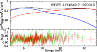
3.1. SWIFT J174540.7-290015
SWIFT J174540.7-290015 (T15 hereafter) is an X-ray transient discovered north of Sagittarius A∗ by Neil Gehrels Swift Observatory on February 6, 2016, and confirmed by Chandra observation taken on 13-14 February 2015, a week after its discovery. T15 was observed by various missions across the whole electromagnetic waveband like XMM-Newton, INTEGRAL/IBIS, and Very large array (VLA). This source was observed for 34 ks by NuSTAR after 16 days of its first detection by Swift, i.e., on February 22, 2016.
The source region is chosen to be a circular region of 30” around the source. For background region, Mori et al. (2019) performed a detailed procedure to assess the effect of other nearby sources present in the background. They found that the background spectra are negligible ( 2%)as compared to the source spectra. Hence, we choose a 30” circular region on the same detector as the background. The spectra are binned to 30 counts per bin to apply chi-square statistics. The extracted spectra have the mean count rate of 6.29 cts-1 (FPMA).
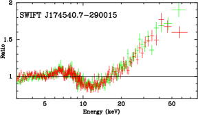
First, we fit the spectra with tbabs*powerlaw to observe the residual features present in the data. Fig. 2 shows the data-to-model ratio for the spectra fit with absorbed power law. The emission around 6-7 keV is visible along with the Compton hump around 20 keV. Absorption at lower energies is also visible. To fit the absorption and the reflection features, we employed the following model (in XSPEC jargon):
| (1) |
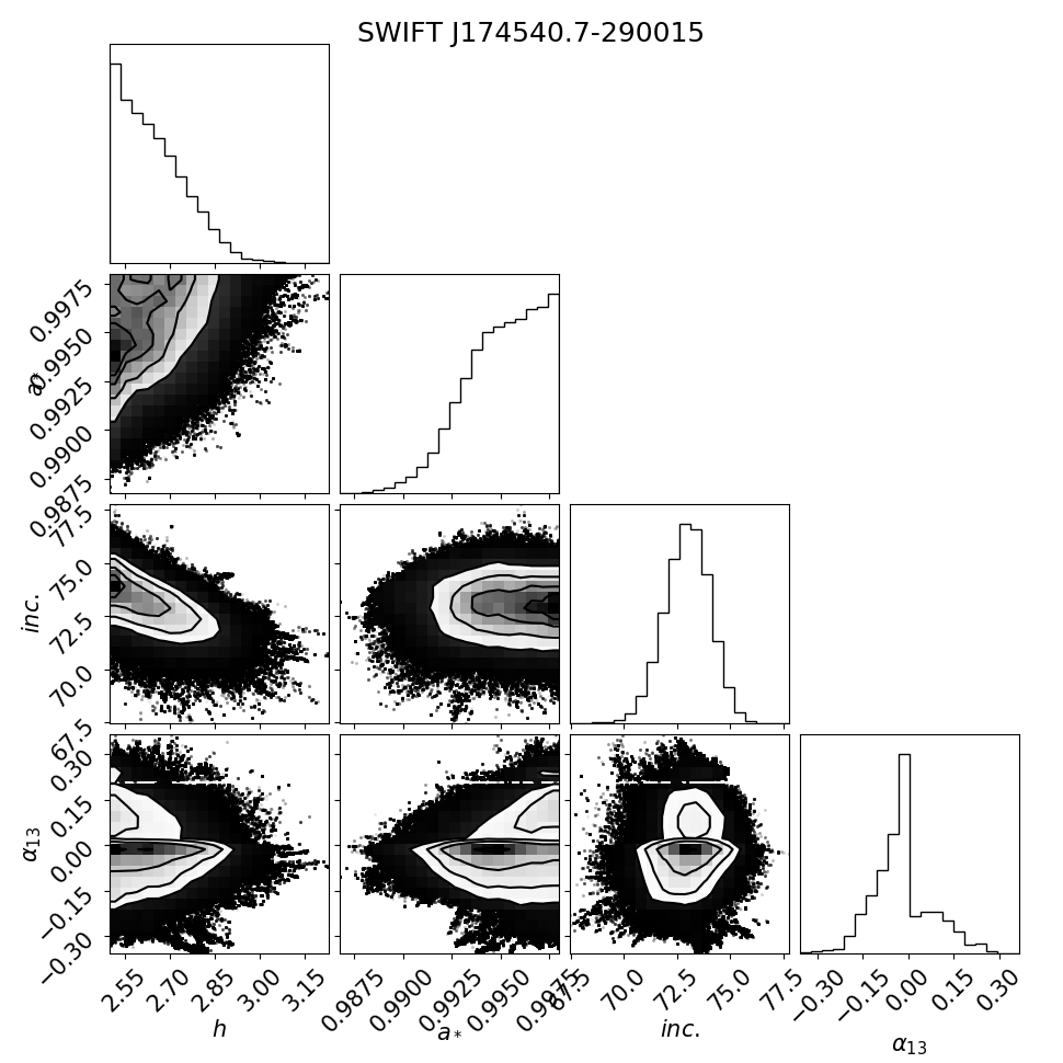
Fig 5 shows the ratio plot for data fitted to the best-fit model. The reduced chi-square is found to be 1.01. Following Mori et al. (2019), we froze the iron abundance at solar value. If the iron abundance is thawed, it gets pegged to unreasonably high values and the spin is loosely constrained. Using the lamppost geometry rather than the broken power-law profile improves the chi-square by 100. The model plot (upper panel of 5) shows that the Comptonized continuum is dominant in the lower energies till 10 keV. After 10 keV, the reflection spectrum, which includes Compton hump as the main feature, begins to dominate till 80 keV. Table 3 shows the errors associated with free parameters. The high absorption nature of this source is reflected in the high value of Tbnew. The high values of spin and inclination angle are found to be consistent with Mori et al. (2019). includes the Kerr solution ( = 0) within 99.73% (3) percentage confidence range. Fig. 6 shows the triangle plot for the posterior distribution of parameters sampled using MCMC analysis. The errors associated with the spin and deformation parameters are given by :
| (2) |


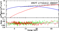
3.1.1 SWIFT J174540.2-290037
SWIFT J174540.2-290037 (T37 hereafter) was discovered by Neil Gehrels Swift Observatory on May 28 2016 when T15 was still in outburst. The X-ray transient is situated south of the Sagittarius A∗ which is confirmed by its Chandra observations and remained bright for a month. It was observed by NuSTAR for 49 ks 16 days after the onset of the outburst on June 16, 2016.
The source region of 30” is taken with the source as the center. For the background spectra, Mori et al. (2019) checked for contamination from other nearby sources and found it to be around 3. So, we neglect the contamination of these sources in extracting the background region. We choose the background region to be of the size of 30” and as far as possible from the source on the same detector. Finally, a binning scheme of 30 counts per bin is employed to make chi statistics applicable. The resultant spectra of the source have an average count rate of 13.6 cts-1 (FPMA).
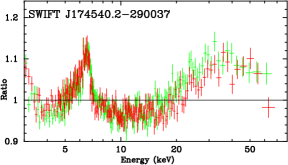
We start the analysis by fitting the spectra with the absorbed power law to highlight the features present in the observation. From Fig. 2, it is clear that the observations consist of an iron line, Compton hump, and a significant absorption at lower energies. We used the following model combination, similar to that of T15, to explain the black hole system :
| (3) |
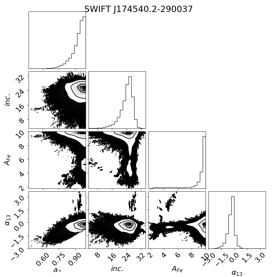
Fig. 5 shows the data fitted to the best-fit model. The upper panel of Fig. 5 shows that the Comptonized continuum continued to be the dominant component till 20 keV. Tab. 3 shows the errors for the parameters of the best-fit model. The reduced is found to be 1.06. This system was also found to have a high spin value as found in the case of T15. However, the inclination angle is lower and the data favors the broken power-law emissivity profile. The inner emissivity index, like most binary systems, is not found to be very steep ( 10), and consequently, the breaking radius is found to be relatively high. The iron abundance is found to be very high which is consistent with the results of Mori et al. (2019). The deformation parameter includes the Kerr solution within 3 significance. Fig. 7 shows the posterior distribution of key parameters obtained by MCMC analysis. The measurements of and is given by
| (4) |
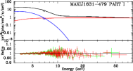
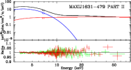
3.1.2 MAXI J1631-479
MAXI J1631-479 is a black hole discovered in 2018 when the source underwent an outburst and situated very close (8.9’) to another X-ray transient AX J1631.9–4752. NuSTAR observed this source on 17, 27, and 29 January 2019 for the duration of 16.3, 10.1, and 14.4 ks respectively. In this case, the source region is 200” centered on the source. The corresponding background region is the annulus region of the inner radius and outer radius to be 200” and 300” respectively. The NuSTAR data is grouped to have a signal-to-noise ratio of 20 counts per bin.
In Observation 1, the source is found to be in disk dominant state where the inner edge of the accretion disk is found to be at the innermost stable circular orbit (ISCO) which is assumed in the calculations involved in relxill_nk. Whereas, the source is found to be in the power law dominant state in Observations 2 and 3. The disk is truncated and the inner edge is not at the ISCO. So, we used Observation 1 for further analysis. Significant spectral variability is found during this observation. The flux is increased by the factor of 3 during this period. We have divided this observation into two parts based on the flux variation to properly account for the variation in spectral analysis. The flux remained constant during the first part (part \Romannum1) and varied during the second part (part \Romannum2).
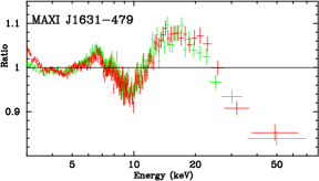
Initially, the spectra are fitted with the combination of disk blackbody emission and power law affected by neutral absorption to inspect the reflection features present in the observation. In XSPEC, the phenomenological model is written as tbabs*(diskbb+powerlaw). In Fig. 2, we can see a broad and asymmetric emission line around 6 keV which corresponds to the iron line and the Compton hump ( 20 keV). In this case, thermal emission dominates up to 10 keV which essentially provides the high energy photons required for ionizing Fe K-shell electron and producing Fe K emission. Therefore, thermal emission is believed to play a major role in Fe fluorescence and in the increase of observed iron line flux which is not possible with coronal illumination alone. Here, the reflection model essentially describes the interaction of the thermal emission of photons with the disk atmosphere rather than the power law continuum. So, the photon index of the power law continuum and the generated reflection spectrum can be different and hence kept free in the fit. We add relxillCp_nk model to account for relativistic reflection. We analyze both parts of the observations simultaneously and link parameters like galactic absorption, spin, inclination, and deformation parameters. Column density of Galactic absorption is kept linked between part \Romannum1 and part \Romannum2 as it is the absorption by interstellar absorption. The temperature of the inner disk radius () is kept free between part \Romannum1 and part \Romannum2. The emissivity from the accretion disk is modeled with broken power law; the inner emissivity index , the outer emissivity index , and the break radius . All parameters of relxill_nk are linked between part \Romannum1 and part \Romannum2 except the ionization parameter (log) because the difference in the flux could result in different ionization parameters of the disk. After the initial fit, there is some absorption visible around 7 keV which is modeled using the XSTAR model. It essentially models the warm absorber into several zones present around the black hole and each zone has characteristic column density and ionization parameter . The warm absorber between part \Romannum1 and part \Romannum2 is first kept free while fitting. The values of these parameters are similar between different parts and therefore, linked for further analysis. It can be motivated by the fact that the warm absorption around the black hole is likely to be unaffected by the variation in X-ray emissions in the inner region of a black hole. In XSPEC, the model can be written as
| (5) |
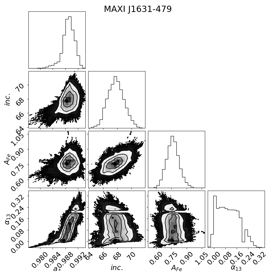
Fig. 5 shows the part \Romannum1 and part \Romannum2 of the observation fitted with the best-fit model. Table 3 reports the uncertainties for each parameter using MCMC simulation and the reduced is 1.28. Very high values of column density and ionization parameter of the XSTAR component indicate the presence of high absorption in the system. The source is found to have a very high spin and inclination angle which is consistent with previous studies (Xu et al., 2020). The emissivity index is found to be 8 () which after 9 , almost becomes almost constant ( 0.12). The iron abundance is found to be sub-solar and has moderate ionization (log 3). Fig. 8 shows the corner plot for the key parameters in the analysis. Deformation parameter includes the Kerr hypothesis with 99.73% confidence. The errors associated with spin and deformation parameter is found to be :
| (6) |
| Parameters | T15 | T37 | MAXI J1631-479 | |
|---|---|---|---|---|
| Part I | Part II | |||
| tbabs | ||||
| [ cm-2] | ||||
| xstar | ||||
| [ cm-2] | - | - | ||
| [erg cm s-1] | - | - | ||
| comptt | ||||
| - | - | |||
| - | - | |||
| - | - | |||
| powerlaw | ||||
| - | - | |||
| diskbb | ||||
| - | - | |||
| relxill(lp)(Cp)_nk | ||||
| - | ||||
| - | ||||
| [] | - | |||
| - | - | - | ||
| [deg] | ||||
| [erg cm s-1] | ||||
| - | - | |||
| (3) | ||||
| 1412/1394 | 2576.50/2432 | 1599.53/1452 | ||
| =1.10133 | =1.0594 | 1.2848 | ||
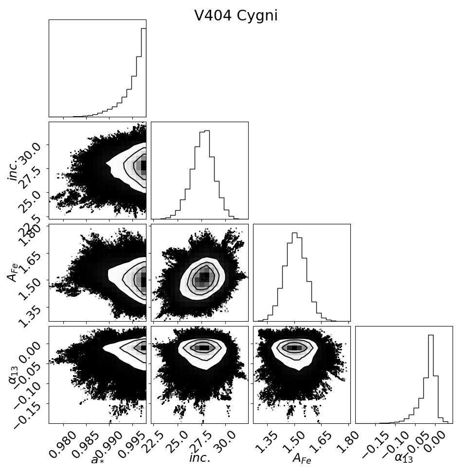
3.1.3 V404 Cyg
V404 Cyg (V404 afterward) is one of the closest black holes ( 2.4 Kpc away) present in a binary system with a K-type stellar companion and has a mass of 9-15 M. It is a low-mass X-ray binary that experienced rare outbursts during which it became the bright X-ray binary in the sky. The first outburst since 1989 from the source was observed in the summer of 2015 which was followed by various multi-wavelength campaigns. NuSTAR observed the source five times after the outburst. In this work, we focus on the first observation which is split into two observation IDs (90102007002 and 90102007003) (Walton et al., 2017). We need to turn off the filtering of a few hot pixels to take into account very high count rates and their rapid variability present throughout the observation. Along with the use of the latest CALDB files which have a database of such hot/flickering pixels, we also used the expression “STATUS=b0000xx00xx0xx000” which controls the filtering. If we don’t use such filtering and use the standard NUPIPELINE routine, then it is possible that some source photons during the flaring process could be eliminated. This filtering will keep these flare photons by not identifying them as hot/flickering. The source region of 160” with the source as the center is taken on a detector. Due to the very bright nature of the source, it is not possible to extract the background region from the same detector. As FPM consists of 4 detectors, the background region is taken from the other detector as far as possible from the source. The FPMA and FPMB data of both Observation IDs are combined separately using the ADDASCASPEC tool and the spectra are binned in such a way that each bin would contain at least 50 counts per bin for the applicability of statistics.
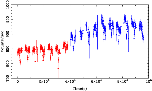
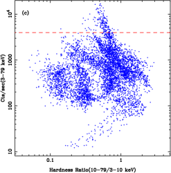
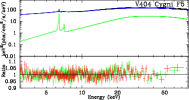
Fig. 4(a) shows the light curve extracted from the NuSTAR observation. The extreme variability can be seen throughout the observation with the count rate exceeding 20,000 counts/sec during the peak flares. The flux observed from the source increased by an order of magnitude very rapidly. The observation also displays spectral variability. Fig. 4(b) shows the progression of hardness ratio which is the ratio of the flux in the hard band (10-79 keV) and soft band (3-10 keV). It shows that the hardness ratio remains almost constant for the first few orbits and then starts to vary rapidly which coincides with the onset of flares in the observation. In Fig. 4(c), we plotted the hardness intensity diagram for this observation which is essentially the hardness ratio plotted against the flux in the whole allowed energy band (3-79 keV). Spectral states are not specifically defined and no correlation is found in the majority of observations. The positive correlation can be seen only at lower count rates up to 100 cts-1 which is very less as compared to the counts during the flares ( cts-1).
| Parameters | F1 | F2 | F3 | F4 | F5 |
|---|---|---|---|---|---|
| tbabs | |||||
| [ cm-2] | |||||
| xstar | |||||
| [ cm-2] | |||||
| [erg cm s-1] | |||||
| relxillCp_nk | |||||
| [] | |||||
| [deg] | |||||
| [keV] | |||||
| [erg cm s-1] | |||||
| (3) | |||||
| 11540.3//10839 = 1.0608 | |||||
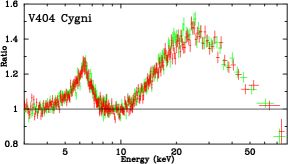
To check the presence of absorption during flares and to highlight the reflection features present in the observation, we have obtained the spectra for which the count rate exceeds 4,000 counts/sec. The total exposure is only about 110 ks and reflection features are clearly visible when it is fitted with the absorbed power law as shown in figure 2. There is also an absorption edge present around 7.5 keV implying that additional absorption is present along with the Galactic one. There is no visible absorption in the flare spectrum. It implies that the flares also originate from the inner region of the accretion disk and the absorption is unlikely to have any significant effect on very high count rates.
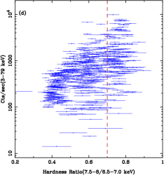
To account for the rapid variability, we perform flux-resolved spectroscopy for this observation. We divide the data into five flux bins. To account for the variable absorption throughout the observation, we select only periods with low absorption based on the flare spectrum. To explain these low-absorption periods, we define a quantity named narrow band hardness ratio () which is essentially the ratio between the softer band (6.5-7.0 keV) and the harder band (7.5-8.0 keV). These bands are chosen such that the softer band is just below the sharp absorption edge observed in the average spectrum and the harder band is just above the sharp edge. This scheme is done to assess the strength of the absorption throughout the observation. In these narrow bands, the strong absorption corresponds to the soft spectrum and lower hardness ratio. Therefore, we need to include the period having higher than a certain threshold which is taken as 0.7. Fig. 4(d) shows the hardness intensity diagram for the hardness defined in the energies range 7.5-8.0 keV and 6.5-7.0 keV. The threshold is denoted by a red dashed line.
We select the data after imposing constraints on flux bins and i.e., we select the data with 0.7 throughout the observation with count rates less than 4,000 cts/sec and then resolve the data in four flux bins: 100-500, 500-1000, 1000-2000, and 2000-4000 cts-1. For the flux bin of more than 4000, we took the whole period as it already has 0.7. So, there are five flux states in total; named as F1-5. The lower limit of the data used in the analysis is 100 cts/sec because, below this, the flux in the broadband is correlated with the hardness ratio.
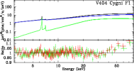
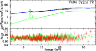
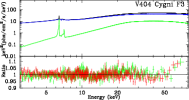
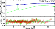
Now, we have five flux states with low absorption. We analyzed all five flux states simultaneously. The model used to describe this black hole system consists of a power-law emission from the corona, reflection spectrum from the disk (both nearby and away from the black hole), galactic absorption, and the intrinsic absorption of the source. In XSPEC, the model is written as :
tbabs*XSTAR*(relxillCp_nk + xillverCp)
The column density of Galactic absorption is kept frozen at cm-3 and is the same for all flux states. Column density and ionization of XSTAR is kept free among different flux states. relxillCp_nk models the Comptonized relativistic reflection model which is coming from the innermost region of the black hole. The broken emissivity profile is used and kept free among different flux states as it is believed that the difference in the flux could be due to different emission rates. Spin (), inclination (), and iron abundance () are tied between various flux levels. The ionization parameter is kept untied between the flux levels as the accretion disk is believed to be ionized differently and produce different flux states. xillverCp models the distant reflector which is essentially not affected by the strong gravity of the central compact object. The incident spectrum that produces both distant non-relativistic and relativistic reflection spectrum is assumed to be produced by the same mechanism and hence the photon index, electron temperature of both relxillCp_nk and xillverCp are tied. As relxillCp_nk includes the continuum, we only include the reflected component from xillverCp which is done by setting the reflection fraction to -1. The accretion disk is assumed to be ”cold” (not ionized enough) at larger distances and hence ionization parameter is frozen to 0. The iron abundance is tied between the relxillCp_nk and xillverCp.
Fig 5 shows the ratio of the data fitted to the best model for all five flux states for V404. Tab. 4 reports the uncertainties on the parameters that are variable during the fit. We obtained a good fit for all five flux states and the combined comes out to be 1.06. The residuals remain after fitting the best model decrease as we go from flux F1 to F5. The column density of the warm absorber is less for high flux states which implies that the absorption affects the spectrum less as the flux increases. The broken emissivity profile used here was found to have very steep inner emissivity (10) and low outer emissivity (3.0) with a break radius in the range 1.5-3.0. The source is found to have a large spin and small inclination angle which agrees with the previous studies of the source. Fig. 9 shows the triangle plot for the posterior distribution of globally defined parameters for the best-fit model. recovers the Kerr solution with 99.73% confidence. The 1 uncertainty associated with spin and deformation parameters for V404 is given by
| (7) |
4. Discussion and conclusions
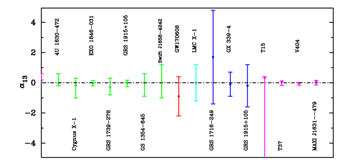
In this work, we have analyzed highly complicated X-ray NuSTAR observations of four X-ray binaries; T15, T37, MAXI J1631–479, and V404. We have used the non-Kerr extension of the state-of-the-art relativistic model to analyze these observations and obtain constraints compared to what was obtained in Tripathi et al. (2021a). Such comparable constraints can only be obtained through advanced reduction techniques applied to the observations like flux-resolved and time-resolved spectroscopy. It is highly crucial to model the warm absorbers and absorption, if present, in the observation which could be very specific in every case. For instance, the flux changed by 15% in a single observation for MAXI J1631–479. We divide the observation such that the variation in each part remains constant and thus accounts for the variability. In V404, multiple flares are present in the observation which are divided into various flux states to account for the increase in flux due to absorption. In addition, we also need to impose 0.7 to analyze the data which is least affected by absorption. We used the version of the galactic absorption model TBnew which deals with heavy absorption. So, adopting such sophisticated data reduction schemes would result in stringent constraints on metric and accretion disk parameters and thus lead to testing general relativity using such highly absorbed X-ray observations.
Fig. 10 shows the 3 confidence interval on the measurement of estimated by analyzing X-ray data of various X-ray binaries (this work and Tripathi et al. (2021a)). We also show the measurement of from the LIGO/Virgo data (Cárdenas-Avendaño et al., 2020). The gravitational event GW170608, shown in Fig. 10, provides the strongest constraint which is comparable with the constraints obtained in this work.
Several assumptions are made in the relativistic reflection models used in this work. We will discuss these simplifications and their potential effects on the results. The disk emissivity profile could be very crucial in determining the appropriate reflection spectrum of a source. In this work, we tried the emissivity profiles included in relxill_nk; simple power law, broken power law, and lampost. We select the best profile yielding minimum likelihood. In relxill_nk, the inner edge of the accretion disk is assumed to be at the innermost stable circular orbit (ISCO). The assumption is valid for the sources in soft states having the Eddington ratio of 0.05–0.3. For the sources in hard states, this assumption is not valid and the disk could truncate at a radius different than ISCO. However, the sources used in this work have very high spin parameters and the inner edge of the disk is very close to ISCO and therefore, has minimum effect on the measurement of . Both relxill_nk and nkbb assume the accretion disk to be infinitesimally thin. In reality, the disk has a finite thickness which could increase with the increase in mass accretion rate. As the sources in this work are maximally rotating, the thickness of the disk has a negligible effect on the measurement of as shown in Abdikamalov et al. (2020).
The current reflection models ignore the effect of the radiation from the plunging region which would not affect the highly rotating sources (as in our work) as they have a very small plunging region (Cárdenas-Avendaño et al., 2020). The relxill_nk version used in this work assumes a constant electron density = which is too low for the X-ray binaries with high mass accretion rate. The sources analyzed in this work have high mass accretion rates and therefore, this effect needs to be explored further. Studies by Zhang et al. (2019) and (Tripathi et al., 2021) conclude that the electron density has a negligible effect on the measurement of .
relxill_nk does not take into account the effect of returning radiation. A fraction of the reflection radiation emitted from the accretion disk returns to the disk due to the strong light-bending effect in the innermost regions of a black hole. Riaz et al. (2023) studied the effect of returning radiation on the reflection spectrum through simulations and found that the current versions of reflection models (without returning radiation) can be used to test the Kerr metric.
Acknowledgments
This work was supported by the Innovation Program of the Shanghai Municipal Education Commission, grant No. 2019-01-07-00-07- E00035, the National Natural Science Foundation of China (NSFC), grant No. 11973019, and Fudan University, grant No.JIH1512604. GM acknowledges the support from the China Scholarship Council (CSC), Grant No. 2020GXZ016647.
References
- Abbott et al. (2016) Abbott, B. P., Abbott, R., Abbott, T. D., et al. 2016, Phys. Rev. Lett., 116, 221101. doi:10.1103/PhysRevLett.116.221101
- Abbott et al. (2019) Abbott, B. P., Abbott, R., Abbott, T. D., et al. 2019, Phys. Rev. D, 100, 104036. doi:10.1103/PhysRevD.100.104036
- Abdikamalov et al. (2019) Abdikamalov, A. B., Ayzenberg, D., Bambi, C., et al. 2019, ApJ, 878, 91. doi:10.3847/1538-4357/ab1f89
- Abdikamalov et al. (2020) Abdikamalov, A. B., Ayzenberg, D., Bambi, C., et al. 2020, ApJ, 899, 80. doi:10.3847/1538-4357/aba625
- Bambi (2017) Bambi, C. 2017, Reviews of Modern Physics, 89, 025001. doi:10.1103/RevModPhys.89.025001
- Bambi (2018) Bambi, C. 2018, Annalen der Physik, 530, 1700430. doi:10.1002/andp.201700430
- Bambi et al. (2021) Bambi, C., Brenneman, L. W., Dauser, T., et al. 2021, Space Sci. Rev., 217, 65. doi:10.1007/s11214-021-00841-8
- Bambi et al. (2017) Bambi, C., Cárdenas-Avendaño, A., Dauser, T., et al. 2017, ApJ, 842, 76. doi:10.3847/1538-4357/aa74c0
- Bambi et al. (2014) Bambi, C., Malafarina, D., & Tsukamoto, N. 2014, Phys. Rev. D, 89, 127302. doi:10.1103/PhysRevD.89.127302
- Brenneman & Reynolds (2006) Brenneman, L. W. & Reynolds, C. S. 2006, ApJ, 652, 1028. doi:10.1086/508146
- Cao et al. (2018) Cao, Z., Nampalliwar, S., Bambi, C., et al. 2018, Phys. Rev. Lett., 120, 051101. doi:10.1103/PhysRevLett.120.051101
- Cárdenas-Avendaño et al. (2020) Cárdenas-Avendaño, A., Nampalliwar, S., & Yunes, N. 2020, Classical and Quantum Gravity, 37, 135008. doi:10.1088/1361-6382/ab8f64
- Cárdenas-Avendaño et al. (2020) Cárdenas-Avendaño, A., Zhou, M., & Bambi, C. 2020, Phys. Rev. D, 101, 123014. doi:10.1103/PhysRevD.101.123014
- Dauser et al. (2013) Dauser, T., Garcia, J., Wilms, J., et al. 2013, MNRAS, 430, 1694. doi:10.1093/mnras/sts710
- Draghis et al. (2020) Draghis, P. A., Miller, J. M., Cackett, E. M., et al. 2020, ApJ, 900, 78. doi:10.3847/1538-4357/aba2ec
- Einstein (1916) Einstein, A. 1916, Annalen der Physik, 354, 769. doi:10.1002/andp.19163540702
- El-Batal et al. (2016) El-Batal, A. M., Miller, J. M., Reynolds, M. T., et al. 2016, ApJ, 826, L12. doi:10.3847/2041-8205/826/1/L12
- García et al. (2014) García, J., Dauser, T., Lohfink, A., et al. 2014, ApJ, 782, 76. doi:10.1088/0004-637X/782/2/76
- García & Kallman (2010) García, J. & Kallman, T. R. 2010, ApJ, 718, 695. doi:10.1088/0004-637X/718/2/695
- Giddings (2017) Giddings, S. B. 2017, Nature Astronomy, 1, 0067. doi:10.1038/s41550-017-0067
- Harrison et al. (2013) Harrison, F. A., Craig, W. W., Christensen, F. E., et al. 2013, ApJ, 770, 103. doi:10.1088/0004-637X/770/2/103
- Herdeiro & Radu (2014) Herdeiro, C. A. R. & Radu, E. 2014, Phys. Rev. Lett., 112, 221101. doi:10.1103/PhysRevLett.112.221101
- Kerr (1963) Kerr, R. P. 1963, Phys. Rev. Lett., 11, 237. doi:10.1103/PhysRevLett.11.237
- Kleihaus et al. (2011) Kleihaus, B., Kunz, J., & Radu, E. 2011, Phys. Rev. Lett., 106, 151104. doi:10.1103/PhysRevLett.106.151104
- King et al. (2014) King, A. L., Walton, D. J., Miller, J. M., et al. 2014, ApJ, 784, L2. doi:10.1088/2041-8205/784/1/L2
- Miller et al. (2013) Miller, J. M., Parker, M. L., Fuerst, F., et al. 2013, ApJ, 775, L45. doi:10.1088/2041-8205/775/2/L45
- Miller et al. (2015) Miller, J. M., Tomsick, J. A., Bachetti, M., et al. 2015, ApJ, 799, L6. doi:10.1088/2041-8205/799/1/L6
- Mitsuda et al. (1984) Mitsuda, K., Inoue, H., Koyama, K., et al. 1984, PASJ, 36, 741
- Mori et al. (2019) Mori, K., Hailey, C. J., Mandel, S., et al. 2019, ApJ, 885, 142. doi:10.3847/1538-4357/ab4b47
- Nandra et al. (2013) Nandra, K., Barret, D., Barcons, X., et al. 2013, arXiv:1306.2307
- Parker et al. (2016) Parker, M. L., Tomsick, J. A., Kennea, J. A., et al. 2016, ApJ, 821, L6. doi:10.3847/2041-8205/821/1/L6
- Parker et al. (2015) Parker, M. L., Tomsick, J. A., Miller, J. M., et al. 2015, ApJ, 808, 9. doi:10.1088/0004-637X/808/1/9
- Psaltis et al. (2020) Psaltis, D., Medeiros, L., Christian, P., et al. 2020, Phys. Rev. Lett., 125, 141104. doi:10.1103/PhysRevLett.125.141104
- Reynolds (2019) Reynolds, C. S. 2019, Nature Astronomy, 3, 41. doi:10.1038/s41550-018-0665-z
- Riaz et al. (2023) Riaz, S., Mirzaev, T., Abdikamalov, A. B., et al. 2023, European Physical Journal C, 83, 838. doi:10.1140/epjc/s10052-023-12031-7
- Ross & Fabian (2005) Ross, R. R. & Fabian, A. C. 2005, MNRAS, 358, 211. doi:10.1111/j.1365-2966.2005.08797.x
- Tao et al. (2019) Tao, L., Tomsick, J. A., Qu, J., et al. 2019, ApJ, 887, 184. doi:10.3847/1538-4357/ab5282
- Titarchuk (1994) Titarchuk, L. 1994, ApJ, 434, 570. doi:10.1086/174760
- Tomsick et al. (2014) Tomsick, J. A., Nowak, M. A., Parker, M., et al. 2014, ApJ, 780, 78. doi:10.1088/0004-637X/780/1/78
- Tripathi et al. (2021) Tripathi, A., Abdikamalov, A. B., Ayzenberg, D., et al. 2021, ApJ, 907, 31. doi:10.3847/1538-4357/abccbd
- Tripathi et al. (2021a) Tripathi, A., Zhang, Y., Abdikamalov, A. B., et al. 2021, ApJ, 913, 79. doi:10.3847/1538-4357/abf6cd
- Tripathi et al. (2019) Tripathi, A., Nampalliwar, S., Abdikamalov, A. B., et al. 2019, ApJ, 875, 56. doi:10.3847/1538-4357/ab0e7e
- Tripathi et al. (2020b) Tripathi, A., Zhou, M., Abdikamalov, A. B., et al. 2020b, ApJ, 897, 84. doi:10.3847/1538-4357/ab9600
- Verner et al. (1996) Verner, D. A., Ferland, G. J., Korista, K. T., et al. 1996, ApJ, 465, 487. doi:10.1086/177435
- Walton et al. (2017) Walton, D. J., Mooley, K., King, A. L., et al. 2017, ApJ, 839, 110. doi:10.3847/1538-4357/aa67e8
- Walton et al. (2016) Walton, D. J., Tomsick, J. A., Madsen, K. K., et al. 2016, ApJ, 826, 87. doi:10.3847/0004-637X/826/1/87
- Will (2014) Will, C. M. 2014, Living Reviews in Relativity, 17, 4. doi:10.12942/lrr-2014-4
- Wilms et al. (2000) Wilms, J., Allen, A., & McCray, R. 2000, ApJ, 542, 914. doi:10.1086/317016
- Xu et al. (2018a) Xu, Y., Harrison, F. A., García, J. A., et al. 2018a, ApJ, 852, L34. doi:10.3847/2041-8213/aaa4b2
- Xu et al. (2018b) Xu, Y., Harrison, F. A., Kennea, J. A., et al. 2018b, ApJ, 865, 18. doi:10.3847/1538-4357/aada03
- Xu et al. (2020) Xu, Y., Harrison, F. A., Tomsick, J. A., et al. 2020, ApJ, 893, 30. doi:10.3847/1538-4357/ab7dc0
- Yagi & Stein (2016) Yagi, K. & Stein, L. C. 2016, Classical and Quantum Gravity, 33, 054001. doi:10.1088/0264-9381/33/5/054001
- Yunes et al. (2016) Yunes, N., Yagi, K., & Pretorius, F. 2016, Phys. Rev. D, 94, 084002. doi:10.1103/PhysRevD.94.084002
- Zhang et al. (2016) Zhang, S. N., Feroci, M., Santangelo, A., et al. 2016, Proc. SPIE, 9905, 99051Q. doi:10.1117/12.2232034
- Zhang et al. (2019) Zhang, Y., Abdikamalov, A. B., Ayzenberg, D., et al. 2019, ApJ, 884, 147. doi:10.3847/1538-4357/ab4271