Hitomi-HXT deconvolution imaging of the Crab Nebula dazzled by the Crab pulsar

Abstract

We develop a new deconvolution method to improve the angular resolution of the Crab Nebula image taken by the Hitomi HXT. Here, we extend the Richardson-Lucy method by introducing two components for the nebula and the Crab pulsar with regularization for smoothness and flux, respectively, and deconvolving multi-pulse-phase images simultaneously. The deconvolved nebular image at the lowest energy band of 3.6–15 keV looks consistent with the Chandra X-ray image. Above 15 keV, we confirm that the NuSTAR’s findings that the nebula size decreases in higher energy bands. We find that the north-east side of the nebula becomes dark in higher energy bands. Our deconvolution method can be applicable for any telescope images of faint diffuse objects containing a bright point source.

1 Introduction

The Crab Nebula is a synchrotron nebula powered by the rotational energy loss of the central pulsating neutron star, the Crab pulsar (Rees and Gunn, 1974; Kennel and Coroniti, 1984). The X-ray image of the nebula with a high angular resolution of arcsec level was obtained by the Chandra X-Ray Observatory below about 10 keV ($0.5$ arcsec; Weisskopf et al. (2000)). It revealed the detailed nebular structure around the Crab pulsar such as torus, inner ring and jets. The torus whose symmetric axis coincides with the pulsar spin axis is seen and the north-west edge is closer to the observer. The jets emerge from the Crab pulsar along the pulsar spin axis outwards into the counter directions of south-east and north-west. Such structures elucidated the magneto-hydrodynamics and particle acceleration in the pulsar wind nebula (e.g., Porth, Komissarov, and Keppens (2014)). The energy dependency of the shape would help to understand the particle acceleration mechanism within the pulsar wind. Above 10 keV, however, the angular resolution is worse than that below 10 keV and the best resolution so far is $18$ arcsec (full width at half maximum; FWHM) and $58$ arcsec (half power diameter; HPD), achieved by the NuSTAR X-ray telescope (Harrison et al. (2013)).

The Hitomi X-ray Observatory was launched in February 2016 and stopped its operation on the end of March (Takahashi et al. (2016)). It carried the hard X-ray imaging spectroscopy system consisting of two pairs of Hard X-ray Imagers (HXI-1 and HXI-2) and Hard X-ray Telescopes (HXT-1 and HXT-2). The HXIs provide images and spectra up to 80 keV with moderate energy resolution (1.0 keV at 13.9 keV and 2.0 keV at 59.5 keV in FWHM; Hagino et al. (2018)). The effective area is about 300 cm² at 30 keV with a field of view of 9 $\times$ 9 arcmin². The angular resolution of the Hitomi HXT was reported to be $\sim 1.6$ arcmin in HPD (Matsumoto et al., 2018). Although it is slightly worse than that of the NuSTAR, we report in this paper that the core of the point spread function (PSF) of the Hitomi HXT we use is smaller than that of the NuSTAR (section 4). So, Hitomi HXT has a potential to obtain better images in angular resolution than that of NuSTAR after image deconvolution.

Image deconvolution is a mathematical technique to improve the angular resolution of telescopes, which utilizes information of the PSF of telescopes. Richardson-Lucy method (Richardson, 1972; Lucy, 1974) is a well-known canonical method for the image deconvolution, which is an iterative computational algorithm to obtain the deconvolved image of the sky with maximal likelihood for the image data, assuming that the detected photon events follow the Poisson distribution. Since the Crab Nebula is a spatially extended and diffuse object, the smoothness in the intensity distribution is a well convincing assumption and useful to reduce the statistical fluctuation. So, the image deconvolution with smoothness and sparseness regularization proposed by Morii, Ikeda, and Maeda (2019) is thought to be applicable for this case. However, the smoothness regularization make the nebula image deteriorate, because the far bright Crab pulsar overlays the nebula image. It motivates us to develop a new deconvolution method special for the Crab Nebula, separating the nebula and pulsar components effectively.

2 Observation data

The Crab Nebula was observed on 2016 March 25 from 12:35 to 18:01 UT during the Hitomi’s commissioning phase. It was imaged at around the center of the HXI array. The observation time span was 21.5 ks, whereas the total on-source time was $\sim 8$ ks. It is the only observation of the Crab Nebula taken by Hitomi. We use the cleaned data (Sequence ID. 100044010 ), made by applying the standard screening (Angelini et al., 2016) with the processing script of the version of 01.01.003.003. To detect the pulsation of the Crab pulsar, the barycentric correction for photon arrival times is applied for the Crab pulsar position of $(\alpha,\delta)_{\rm J2000}=(83.6332208,22.0144614)$ (Mori et al. (2004) and reference therein).

We use all the cleaned data for HXI-1, whereas we use only the hard band data above 15 keV for HXT-2. It is because one of HXI-2’s readout strips near the aimpoint was a bit noisy, making a bad line in the image, and has no sensitivity below $\sim 10$ keV. In what follows, we divide the HXI data into three energy bands: 3.6–15, 15–30 and 30–70 keV. The total counts within the square region with $80\times 80$ pixels centered on the Crab pulsar are summarized in table 1. The images in the lowest energy band of 3.6–15 keV have rich sample of photons over million counts, whereas the highest energy band images above 30 keV have less sample of photons of forty thousands.

Table 1: Counts detected in the energy bands of HXIs

Detector	HXI-1			HXI-2			Note
	Energy band (keV–keV)			Energy band (keV–keV)
Phase ID	3.6–15	15–30	30–70	3.6–15	15–30	30–70
ALL	1 696 836	223 323	43 878	1 545 317	204 465	39 940
ON2	462 350	62 520	12 564	418 696	57 225	11 490	Secondary peak
OFF1	613 895	78 346	14 953	562 049	71 508	13 649	Off-pulse
ON1	375 538	50 197	9 926	341 238	45 754	8 817	Primary pulse
OFF2	245 053	32 260	6 435	223 334	29 978	5 984

In order to estimate the non X-ray background level, we analyze a blank sky data since the non X-ray background dominates the cosmic X-ray background in flux (Hagino et al., 2018). As listed in Hagino et al. (2018), RX J1856.5$-$3754 has no significant flux above 2 keV and is regarded as a blank sky for our purpose. We combine the cleaned RX J1856.5$-$3754 data with the sequence IDs of 100043010, 100043020, 100043030, 100043040 and 100043050, and make images of 80 $\times$ 80 pixels in the sky coordinate for each energy band. The total exposure time of RX J1856.5$-$3754 was 102 ks for HXIs. The estimated counts of non X-ray background per 8 ks are 11(16), 9(10) and 40(40) in the energy bands of $3.6-15$, $15-30$ and $30-70$ keV for HXI-1 (HXI-2), respectively. They are negligibly small for our purpose.

3 Point spread function

Figure 1: Folded light curve of the HXI-1 in all the energy band.

For the image deconvolution, the model of the PSF dependent on energy and in-coming directions of photons (response matrix) is necessary. Due to the Hitomi’s short life, the PSF is not well modeled and the dependency on the direction is also not measured. However, at least for the Crab Nebula, a reliable PSF is obtained for the in-coming direction from the Crab pulsar as demonstrated by Matsumoto et al. (2018). We here follow their method to make the PSF.

The Crab pulsar exhibits X-ray pulsation with a period of $\sim 34$ ms, and the pulse profile has a double peak structure (Ducros et al., 1970). Since the HXI has a time resolution of $25.6~{}\mu{\rm s}$ (Nakazawa et al., 2018), the pulsation was successfully detected by the HXI as reported by Hitomi Collaboration et al. (2018). Figure 1 shows such a pulse profile of the Crab pulsar, made by folding the HXI-1 light curve with the pulse period of 33.7204626 ms at 57472.5 d (MJD), which is the phase zero. We define the pulse phases ON1, OFF2, ON2 and OFF1 by the durations of $0.504-0.704$, $0.704-0.854$, $0.854-1.104$ and $0.104-0.504$, respectively. Table 1 shows the counts in each pulse phase. Then, by subtracting the image in the OFF1 phase from the ON phase (the addition of the ON1 and ON2 phases), we can obtain the Crab pulsar image, which is just the PSF we need for the image deconvolution. We use the square region with $80\times 80$ pixels centered on the Crab pulsar for the PSF.

Since this PSF is obtained from the observed data itself, the pointing instability of the telescope during the observation does not cause the uncertainty of the PSF. We adapt the same PSF for the directions other than the central pulsar direction. In section 13, we discuss the causes of uncertainty of the PSF and evaluate the effect of them for the deconvolved image.

4 Sharpness of the PSF

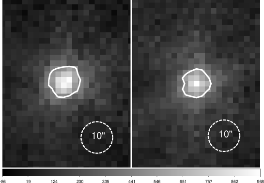
Figure 2: The Crab pulsar images of HXI-1 (left) and HXI-2 (right). They are made by subtracting the OFF-pulse image from the ON-pulse image (see text for details). The pixel size of the image is 1.77 arcsecs. The contours are drawn at the half of each peak counts. The diameters of the dashed circles are 10 arcsecs.

Table 2: FWHM of the Crab pulsar images

	HXI-1		HXI-2
Energy band	FWHM	Maximum pixel	FWHM	Maximum pixel
(keV–keV)	(arcsec)	(counts/pixel)	(arcsec)	(counts/pixel)
All band	10	1012	9	967
3.6-15	10	852	8	813
15-30	10	138	10	131
30-70	5	43	7	34

Since the sharpness of the PSF core contributes the goodness of an angular resolution of deconvolved images, we here evaluate it as the FWHM of the PSF. Figure 2 shows the Crab pulsar images of HXIs without smoothing nor binning, for which no energy filtering are applied. The counts at the peak pixels are 1012 and 967 for HXI-1 and HXI-2, respectively. The contours depict the position of the half of the peaks. Before drawing these contours, we applied a Gaussian smoothing with one sigma width of one pixel, to draw the contours in sub-pixel resolution. We calculate the FWHM as the equivalent diameter of the circle whose area is the same as the enclosed area by the contour. The FWHMs of the PSFs are 10 and 9 arcsecs for HXI-1 and HXI-2, respectively. They are about a half of the PSF of the NuSTAR telescope (18 arcsecs : Harrison et al. (2013)). The FWHMs of the PSFs for three energy bands are shown in table 2.

5 Mathematical formulation of the problem

Hitomi satellite has two hard X-ray telescopes (HXT-1, HXT-2) with photon counters (HXI-1, HXI-2) at their respective foci. We consider a rectangular area on the tangential plane of the celestial sphere as an observed image by the Hitomi HXT/HXI system. The area is divided into $M=m\times n$ pixels ($m=100,n=100$), where each pixel is indexed with $u=(i,j)$ ($i=1,\cdots,m;j=1,\cdots,n$). The image is expressed by the distribution of intensity of photons $I_{u}$ per each pixel $u$, by a non-negative real value. Pixels of HXI is indexed with $v$ ($v=1,\cdots,V$; $V=80\times 80$). The HXI-1 and HXI-2 are identified with $c=1,2$, respectively, and the number of counters is $n_{c}=2$. The events detected at a pixel $v$ of HXI ($c$) consist of both X-ray photons through Hitomi-HXT/HXI system and charged particles which directly hit on the pixel. The number of these events in an exposure (an observation) of Hitomi-HXT/HXI is $Y_{c,v}$, which is a non-negative integer value. It follows a Poisson distribution:

$$Y_{c,v}\sim{\rm Poisson}\left(\sum_{u}t_{c,v,u}I_{u}+b_{c,v}\right),$$ (1)

where $t_{c,v,u}$ is the response of the Hitomi-HXT/HXI. It means a distribution of the expected photon counts at pixel $v$ of counter $c$ from a pixel $u$ with a unit intensity at the celestial sphere, that is the PSF. Here, $b_{c,v}$ is the particle background counts at pixel $v$ of the counter $c$ as a non-negative real value.

The detection efficiency ($\epsilon_{u}$) of photons by the counters from a celestial pixel $u$ follows a relation $\sum_{c,v}t_{c,v,u}=\epsilon_{u}\leq 1$. Here, the effects of vignetting of HXTs and quantum efficiency of HXIs are included in the factor $\epsilon_{u}$. Assuming $0<\epsilon_{u}\leq 1$, and setting $t^{\prime}_{c,v,u}=t_{c,v,u}/\epsilon_{u}$ and $I^{\prime}_{u}=\epsilon_{u}I_{u}$, the equation (1) becomes

$$Y_{c,v}\sim{\rm Poisson}\left(\sum_{u}t^{\prime}_{c,v,u}I^{\prime}_{u}+b_{c,v}\right),$$ (2)

and $t^{\prime}_{c,v,u}$ follows $\sum_{c,v}t^{\prime}_{c,v,u}=1$. So, we solve for $I^{\prime}_{u}$ and $I_{u}$ is then obtained by $I_{u}=I_{u}^{\prime}/\epsilon_{u}$. Hereafter, we thus replace $t^{\prime}_{c,v,u}\rightarrow t_{c,v,u}$ and $I_{u}^{\prime}\rightarrow I_{u}$, so $\sum_{c,v}t_{c,v,u}=1$ is satisfied.

6 Case of the Crab Nebula with the Crab pulsar

We derive the mathematical formulation for the case of the Crab Nebula with the Crab pulsar. Remarks of this case are the followings: (1) The Crab pulsar is a bright point source locating at the center of the Crab Nebula. Its intensity is concentrated at one pixel and far brighter than those of the surrounding nebula. (2) Intensity of the Crab pulsar changes periodically in the pulse period of $\sim 34$ ms with large variation. Due to the first one, we have to assume two components for the celestial image. To decouple these intensities at the pulsar position, we assume spatial smoothness of the nebula component. Utilizing the second point, decoupling of two components is clarified further by introducing a simultaneous image deconvolution using the images of all pulse phases at once, with the nebula component common in all phases and only the intensity of the pulsar varied.

We divide observed data into $n_{p}$ pulse phases ($n_{p}=10$), then we obtain $n_{p}$ images observed by the Hitomi HXT. Pulse phases are indexed with $p=1,2,\cdots,n_{p}$, and the ratio of the time width of the phase $p$ to the pulse period is $(\Delta\phi)_{p}$, where $0<(\Delta\phi)_{p}\leq 1$ and $\sum_{p=1}^{n_{p}}(\Delta\phi)_{p}=1$. In the case of equivalent time width for phases, $(\Delta\phi)_{p}=1/n_{p}$. We express the image of the Crab Nebula by $I_{u}$ and the Crab pulsar by $I_{0,u}$. Here, the value of $I_{0,u}$ is one at the position of the Crab pulsar, and zero at the other positions. The intensity of the Crab pulsar at phase $p$ is expressed by $f_{p}$.

Table 3: Livetime fraction in each pulse phase

Phase	HXI-1	HXI-2
0.0-0.1	0.751	0.736
0.1-0.2	0.782	0.768
0.2-0.3	0.784	0.770
0.3-0.4	0.784	0.770
0.4-0.5	0.783	0.769
0.5-0.6	0.754	0.737
0.6-0.7	0.741	0.726
0.7-0.8	0.774	0.759
0.8-0.9	0.768	0.754
0.9-1.0	0.742	0.726

Due to the limitation of the HXI capability, HXIs have deadtime in an observing duration, which tends to be larger for higher event rates. Thus, deadtimes vary in pulse phases. The livetime is the complement of the deadtime during an observing duration. Table 3 shows the livetime fractions of observing data of the Crab Nebula, calculated by the method given in the appendix of Matsumoto et al. (2018). We set the fraction of the livetime to an exposure of pulse phase $p$ for HXI $c$ to be $(F_{\rm lt})_{c,p}$ ($0\leq(F_{\rm lt})_{c,p}\leq 1$).

The number of events in the pixel $v$ of the counter $c$ in an exposure of a pulse phase $p$ is $Y_{c,p,v}$, which is a non-negative integer value. It follows a Poisson distribution:

$$Y_{c,p,v}\sim{\rm Poisson}\left\{\left[\sum_{u}t_{c,v,u}(I_{u}+f_{p}I_{0,u})+b_{c,v}\right](\Delta\phi)_{p}(F_{\rm lt})_{c,p}\right\}.$$ (3)

Thus, the likelihood of detecting $Y$ events given $I$ and $f$ is expressed as follows:

$$p(Y|I,f)=\prod_{c=1}^{n_{c}}\prod_{p=1}^{n_{p}}\prod_{v=1}^{V}{\rm Poisson}\left\{Y_{c,p,v};\left[\sum_{u}t_{c,v,u}(I_{u}+f_{p}I_{0,u})+b_{c,v}\right](\Delta\phi)_{p}(F_{\rm lt})_{c,p}\right\}.$$ (4)

7 Regularization

We introduce a smoothness constraint for the nebula component $I_{u}$ to reduce statistical fluctuation and to decouple the nebula and pulsar components at the pulsar position. In addition, to stabilize the nebula image around the pulsar position, we also introduce the flux constraint for the pulsar flux $f_{p}$. Such constraints are expressed by prior probabilities in Bayesian inference. The prior for $I_{u}$ is

$$p_{\rm smooth}(I)=Z_{I}\exp[-\mu V(I)],$$ (5)

where

$$V(I) = \sum_{(r,s)\in N}(I_{r}-I_{s})^{2}$$ (6)

$$= \sum_{i=1}^{m-1}\sum_{j=1}^{n-1}\left[(I_{i,j}-I_{i+1,j})^{2}+(I_{i,j}-I_{i,j+1})^{2}\right]$$

$$+\sum_{i=1}^{m-1}(I_{i,n}-I_{i+1,n})^{2}+\sum_{j=1}^{n-1}(I_{m,j}-I_{m,j+1})^{2}.$$

Here, $Z_{I}$ is a normalization constant. $\sum_{(r,s)\in N}$ denotes the summation between two adjoining pixels. $\mu>0$ is a hyper-parameter to control the smoothness of the nebula image.

The prior for $f_{p}$ is

$$p_{\rm flux}(f)=Z_{f}\exp[-\gamma D(f)],$$ (7)

where

$$D(f)=\sum_{p}(f_{p}-f_{0,p})^{2}.$$ (8)

Here, $Z_{f}$ is a normalization constant. $\gamma>0$ is a hyper-parameter to make the flux be close to the pulsed flux of the Crab pulsar $f_{0,p}$. Because Hitomi HXT cannot resolve the Crab pulsar and the nebula on the image, we here use the pulsed flux instead of the unknown total flux. The $\gamma$ parameter works to adjust the difference between the pulsed and total fluxes of the Crab pulsar. The pulsed flux $f_{0,p}$ is obtained by

$$f_{0,p}=\frac{1}{(\Delta\phi)_{p}}\sum_{c}\frac{\sum_{v}Y_{c,p,v}}{(F_{\rm lt})_{c,p}}-\frac{1}{(\Delta\phi)_{\rm off}}\sum_{c}\frac{\sum_{v}Y_{c,{\rm off},v}}{(F_{\rm lt})_{c,{\rm off}}},$$ (9)

where off is the pulse minimum phase.

Then, the posterior is obtained by

$$p(I,f|Y) = \frac{p(I,f,Y)}{p(Y)}=\frac{p_{\rm smooth}(I)p_{\rm flux}(f)p(Y|I,f)}{p(Y)}.$$ (10)

We solve $I$ and $f$ by maximizing the logarithm of $p(I,f|Y)$ ($=-L_{\rm cost}(I,f)$):

$$\log p(I,f|Y) = \log p(Y|I,f)+\log p_{\rm smooth}(I)+\log p_{\rm flux}(f)+{\rm const.}$$ (11)

$$= \log p(Y|I,f)-\mu V(I)-\gamma D(f)+{\rm const}.$$

8 Optimization of the likelihood part $p(Y|I,f)$

We use the EM (Expectation-Maximization) algorithm (Bishop, 2006; Dempster, Laird, and Rubin, 1977) to maximize the likelihood part $p(Y|I,f)$. In this frame work, $p(Y|I,f)$ is called observed likelihood. The corresponding complete likelihood is expressed by

$$p_{\rm complete}(Y,z,w,e|I,f) = \prod_{c=1}^{n_{c}}\prod_{p=1}^{n_{p}}\prod_{v=1}^{V}\left\{\prod_{u=1}^{M}{\rm Poisson}\left[z_{c,p,v,u};t_{c,v,u}I_{u}(\Delta\phi)_{p}(F_{\rm lt})_{c,p}\right]\right.$$ (12)

$$\times{\rm Poisson}\left[w_{c,p,v};f_{p}d_{0,c,v}(\Delta\phi)_{p}(F_{\rm lt})_{c,p}\right]$$

$$\times{\rm Poisson}\left[e_{c,p,v};b_{c,v}(\Delta\phi)_{p}(F_{\rm lt})_{c,p}\right]$$

$$\left.\times\chi_{\{Y_{c,p,v}=\sum_{u}z_{c,p,v,u}+w_{c,p,v}+e_{c,p,v}\}}(z,w,e)\right\},$$

where $z_{c,p,v,u}$, $w_{c,p,v}$ and $e_{c,p,v}$ are latent variables. $z_{c,p,v,u}$ is the photon counts in the pulse phase $p$ at the pixel $v$ of the detector $c$ through the Hitomi-HXT/HXI system from the celestial pixel $u$ of the nebula component. $w_{c,p,v}$ is the same photon counts from the pulsar component. $e_{c,p,v}$ is the counts of charged particles in the pulse phase $p$ at the pixel $v$ of the detector $c$. $d_{0,c,v}=\sum_{u}t_{c,v,u}I_{0,u}$ is the image of the Crab pulsar on the counter $c$. $\chi_{A}$ is the indicator function of a set $A$. Indeed, $p_{\rm complete}(Y,z,w,e|I,f)$ is the complete likelihood, because it satisfies the following:

$$p_{\rm observed}(Y|I,f)=\sum_{z,w,e}p_{\rm complete}(Y,z,w,e|I,f).$$ (13)

So, the $r$-th iterative step of the EM algorithm is derived to be

$$(I,f)^{(r+1)} = \mathop{\rm arg~{}max}\limits_{(I,f)}{\cal L}\left[p(z,w,e|Y,I^{(r)},f^{(r)}),(I,f)\right]$$ (14)

$$= \mathop{\rm arg~{}max}\limits_{(I,f)}\sum_{(z,w,e);p(z,w,e|Y,I^{(r)},f^{(r)})\neq 0}p(z,w,e|Y,I^{(r)},f^{(r)})\log\frac{p(z,w,e,Y|I,f)}{p(z,w,e|Y,I^{(r)},f^{(r)})}$$

$$= \mathop{\rm arg~{}max}\limits_{(I,f)}\sum_{(z,w,e);p(z,w,e|Y,I^{(r)},f^{(r)})\neq 0}p(z,w,e|Y,I^{(r)},f^{(r)})\log p(z,w,e,Y|I,f)$$

$$= \mathop{\rm arg~{}max}\limits_{(I,f)}\log p(z^{(r)},w^{(r)},e^{(r)},Y|I,f),$$

where

$${\cal L}\left[p(z,w,e),(I,f)\right]=\sum_{(z,w,e);p(z,w,e)\neq 0}p(z,w,e)\log\frac{p(z,w,e,Y|I,f)}{p(z,w,e)}$$ (15)

is an infimum function for $\log p_{\rm observed}(Y|I,f)$, and

$$z_{c,p,v,u}^{(r)} = \sum_{z,w,e}p(z,w,e|Y,I^{(r)},f^{(r)})z_{c,p,v,u}=\frac{Y_{c,p,v}t_{c,v,u}I_{u}^{(r)}}{D_{c,p,v}^{(r)}}=Y_{c,p,v}^{\prime(r)}t_{c,v,u}I_{u}^{(r)},$$ (16)

$$w_{c,p,v}^{(r)} = \sum_{z,w,e}p(z,w,e|Y,I^{(r)},f^{(r)})w_{c,p,v}=\frac{Y_{c,p,v}f_{p}^{(r)}d_{0,c,v}}{D_{c,p,v}^{(r)}}=Y_{c,p,v}^{\prime(r)}f_{p}^{(r)}d_{0,c,v},$$ (17)

$$e_{c,p,v}^{(r)} = \sum_{z,w,e}p(z,w,e|Y,I^{(r)},f^{(r)})e_{c,p,v}=\frac{Y_{c,p,v}b_{c,v}}{D_{c,p,v}^{(r)}}=Y_{c,p,v}^{\prime(r)}b_{c,v},$$ (18)

$$D_{c,p,v}^{(r)} = \sum_{u^{\prime}}t_{c,v,u^{\prime}}I_{u^{\prime}}^{(r)}+f_{p}^{(r)}d_{0,c,v}+b_{c,v},$$ (19)

$$Y_{c,p,v}^{\prime(r)} = \frac{Y_{c,p,v}}{D_{c,p,v}^{(r)}}.$$ (20)

9 Optimization of the $V(I)$ part

We apply the MM (Majorization-Minimization) algorithm (Hunter and Lange, 2000) to optimize the $V(I)$ part as shown in Zhou, Alexander, and Lange (2011). A surrogate function for $V(I)$, that is a supremum for $V(I)$, is given by

$$u(I;I^{\prime})=\frac{1}{2}\sum_{(r,s)\in N}\left\{\left[2I_{r}-(I_{r}^{\prime}+I_{s}^{\prime})\right]^{2}+\left[2I_{s}-(I_{r}^{\prime}+I_{s}^{\prime})\right]^{2}\right\}.$$ (21)

Here, the relations

$$V(I) = \sum_{(r,s)\in N}(I_{r}-I_{s})^{2}\leq\frac{1}{2}\sum_{(r,s)\in N}\left\{\left[2I_{r}-(I_{r}^{\prime}+I_{s}^{\prime})\right]^{2}+\left[2I_{s}-(I_{r}^{\prime}+I_{s}^{\prime})\right]^{2}\right\}$$ (22)

$$= u(I;I^{\prime})$$

and

$$V(I)=u(I;I)$$ (23)

hold. So, this part can be optimized by the following update:

$$I^{(t+1)}=\mathop{\rm arg~{}min}\limits_{I}u(I;I^{(t)}).$$ (24)

10 Optimization of $\log p(I,f|Y)$

Combining optimization for both the likelihood and prior parts, the $r$-th updating rule becomes

$$(I^{(r+1)},f^{(r+1)}) = \mathop{\rm arg~{}min}\limits_{(I,f)}u_{\rm cost}(I,f;I^{(r)},f^{(r)})$$ (25)

$$= \mathop{\rm arg~{}min}\limits_{(I,f)}\left\{-{\cal L}\left[p(z,w,e|Y,I^{(r)},f^{(r)}),(I,f)\right]+\mu u(I;I^{(r)})+\gamma D(f)\right\}$$

$$= \mathop{\rm arg~{}min}\limits_{(I,f)}\left[-\sum_{(z,w,e);p(z,w,e|Y,I^{(r)},f^{(r)})\neq 0}p(z,w,e|Y,I^{(r)},f^{(r)})\log p(z,w,e,Y|I,f)\right.$$

$$+\left.\mu u(I;I^{(r)})+\gamma D(f)\right]$$

$$= \mathop{\rm arg~{}min}\limits_{(I,f)}\left[-\sum_{c,p,v}\left(\sum_{u}\left\{z_{c,p,v,u}^{(r)}\log I_{u}-[t_{c,u,v}I_{u}(\Delta\phi)_{p}(F_{\rm lt})_{c,p}]\right\}\right.\right.$$

$$\left.\left.+w_{c,p,v}^{(r)}\log f_{p}-[f_{p}d_{0,c,v}(\Delta\phi)_{p}(F_{\rm lt})_{c,p}]\right)+\mu u(I;I^{(r)})+\gamma D(f)\right],$$

where

$$u_{\rm cost}(I,f;I^{\prime},f^{\prime})=-{\cal L}\left[p(z,w,e|Y,I^{\prime},f^{\prime}),(I,f)\right]+\mu u(I;I^{\prime})+\gamma D(f)$$ (26)

is an supremum function for $L_{\rm cost}(I,f)$. Therefore, each iterative step becomes the following minimization problem:

$$\min_{(I,f)\in R^{M+n_{p}}} \left[-\sum_{c,p,v}\left(\sum_{u}\left\{z_{c,p,v,u}^{(r)}\log I_{u}-[t_{c,u,v}I_{u}(\Delta\phi)_{p}(F_{\rm lt})_{c,p}]\right\}\right.\right.$$

$$\left.\left.+w_{c,p,v}^{(r)}\log f_{p}-[f_{p}d_{0,c,v}(\Delta\phi)_{p}(F_{\rm lt})_{c,p}]\right)\right.$$

$$\left.+\mu u(I;I^{(r)})+\gamma D(f)\right]$$

$$s.t.$$

$$-I_{u} \leq 0\,\,\,\,(u=1,\cdots,M),$$

$$-f_{p} \leq 0\,\,\,\,(p=1,\cdots,n_{p}).$$

If at least one value among $I_{u}$ and $f_{p}$ is zero, the value of equation (10) becomes infinity. So, $I_{u}\neq 0$ and $f_{p}\neq 0$. By using KKT (Karush-Kuhn-Tucker) condition (Bishop, 2006; Kanamori et al., 2016) and introducing Lagrange multipliers $\mu_{u}$ and $\tau_{p}$ ($u=1,\cdots,M$, $p=1,\cdots,n_{p}$), we get the following relations:

$$-m_{u}^{(r)}\frac{1}{I_{u}}+\mu\frac{\partial u(I;I^{(r)})}{\partial I_{u}}+\overline{\epsilon_{u}}-\mu_{u} = 0,$$ (28)

$$-n_{p}^{(r)}\frac{1}{f_{p}}+\gamma\frac{\partial D(f)}{\partial f_{p}}+\overline{d_{p}}-\tau_{p} = 0,$$ (29)

$$\mu_{u}I_{u} = 0,$$ (30)

$$\tau_{p}f_{p} = 0,$$ (31)

$I_{u}\geq 0$, $f_{p}\geq 0$, $\mu_{u}\geq 0$, and $\tau_{p}\geq 0$ $(u=1,\cdots,M,\,\,\,p=1,\cdots,n_{p})$. Here,

$$\overline{\epsilon_{u}} = \sum_{c,p,v}t_{c,v,u}(\Delta\phi)_{p}(F_{\rm lt})_{c,p},$$ (32)

$$\overline{d_{p}} = \sum_{c,v}d_{0,c,v}(\Delta\phi)_{p}(F_{\rm lt})_{c,p},$$ (33)

$$m_{u}^{(r)} = \sum_{c,p,v}z_{c,p,v,u}^{(r)}=\sum_{c,p,v}Y_{c,p,v}^{\prime(r)}t_{c,v,u}I_{u}^{(r)},$$ (34)

$$n_{p}^{(r)} = \sum_{c,v}w_{c,p,v}^{(r)}=\sum_{c,v}Y_{c,p,v}^{\prime(r)}f_{p}^{(r)}d_{0,c,v}.$$ (35)

We obtain $\mu_{u}=0$($u=1,\cdots,M$) and $\tau_{p}=0$($p=1,\cdots,n_{p}$) from equations (30,31), because $I_{u}\neq 0$ and $f_{p}\neq 0$. By the calculation of appendix A, the derivative of $u(I;I^{(r)})$ can be written by

$$\frac{\partial u(I;I^{(r)})}{\partial I_{u}}=\alpha_{u}I_{u}-\beta_{u}^{(r)}.$$ (36)

Finally, from equations (28, 29), we obtain the updating rule for $I_{u}$ and $f_{p}$:

$$I_{u}^{(r+1)}=\frac{1}{2\mu\alpha_{u}}\left\{-(\overline{\epsilon_{u}}-\mu\beta_{u}^{(r)})+\left[(\overline{\epsilon_{u}}-\mu\beta_{u}^{(r)})^{2}+4\mu\alpha_{u}m_{u}^{(r)}\right]^{1/2}\right\},$$ (37)

$$f_{p}^{(r+1)}=\frac{1}{4\gamma}\left\{-\left(\overline{d_{p}}-2\gamma f_{0,p}\right)+\left[\left(\overline{d_{p}}-2\gamma f_{0,p}\right)^{2}+8\gamma n_{p}^{(r)}\right]^{1/2}\right\}.$$ (38)

Then, we can solve this minimization problem by the iterative updating calculation for a fixed ($\mu$, $\gamma$).

We show in appendix B a proof that our algorithm converges to the unique maximum value from any feasible initial value ($I^{(0)},f^{(0)}$) such that $\log p(I^{(0)},f^{(0)}|Y)$ is a finite value.

11 Cross-validation of hyper-parameters

Since the deconvolved image depends on the hyper-parameters ($\mu$, $\gamma$; see figure 3 for example), we then need determine the parameters by the cross-validation as follows. We apply five-fold cross-validation, in which the image data are randomly divided into five sub-data with equivalent photon counts and five pairs of training and validation data are made, where the training one is made up of four sub-data and the validation one is made up of the remaining sub-data. Then, for each pair, the nebula image and pulsar fluxes are obtained by the deconvolution using one of training data and the quality is evaluated against the corresponding validation data. We use the root mean squared error (RMSE) between the image on the detector convolved for the deconvolved image made from one of training data and the corresponding validation data. Here, the RMSE is calculated to be

$${\rm RMSE}=\left\{\frac{\sum_{p=1}^{n_{p}}\sum_{c=1}^{n_{c}}\left[({\rm RMSE})_{c,p}\right]^{2}}{n_{c}n_{p}}\right\}^{1/2},$$ (39)

where

$$({\rm RMSE})_{c,p} = \left(\frac{1}{V}\sum_{v=1}^{V}\left\{\frac{1}{N_{\rm fold}-1}\left[\sum_{u}t_{c,v,u}(I_{u}^{(\rm deconv)}+f_{p}^{(\rm deconv)}I_{0,u})+b_{c,v}\right](\Delta\phi)_{p}(F_{\rm lt})_{c,p}\right.\right.$$ (40)

$$\left.\left.-Y_{c,v}^{(\rm val)}\right\}^{2}\right)^{1/2},$$

and $N_{\rm fold}=5$. $I_{u}^{(\rm deconv)}$, $f_{p}^{(\rm deconv)}$, and $Y_{c,v}^{(\rm val)}$ are the deconvolved nebula image, the pulsar flux, and the validation data, respectively. The average and variance of the RMSE are calculated over the five training-validation data pairs. The evaluation is repeated for each hyper-parameter pair ($\mu$, $\gamma$).

The $\gamma$ parameter mainly affect the pulsar flux and has little effect on the nebula image (figure 3). We then adapt the parameter with the smallest RMSE for this parameter. For the $\mu$ parameter instead of adapting at the smallest RMSE, we adapt the one-standard error rule to avoid the over-training for the training data [for example, Hastie, Tibshirani, and Wainwright (2015)]. In this rule, we adapt the largest $\mu$ (the smoothest) parameter, allowed within the fluctuation of the RMSE. In other words, we adapt the $\mu$ value at which the RMSE is the same as the value obtained by the addition of the minimum RMSE and the one-standard error of RMSE at the $\mu$ with the minimum RMSE. We search the parameter among 121 pairs of ($\mu$, $\gamma$), where $\log_{10}\mu$ and $\log_{10}\gamma$ are varied from $-10$ to $0$ by a step of $1$.

We implement the above algorithm with C++, utilizing the BLAS library . For each fixed hyper-parameter ($\mu$, $\gamma$), we start the deconvolution calculation from an initial value ($I^{(0)},f^{(0)}$) of a flat image and a constant pulse profile, and the updating calculation stops after 10000 iterations or when the Hellinger distance between the current and previous images becomes less than $10^{-7}$. The processing speed is measured by using a computer equipped with CPUs of AMD EPYC 7543. It has 32 cores and the clock is 2.8 GHz. The nebula image with $100\times 100$ pixels and 10 pulse-phase fluxes are deconvolved by an average of 755 s with one standard deviation of 244 s for each hyper-parameter, when using 1 core. For the fast computation, we use CUDA working on GPU (NVIDIA RTX A4000), then mark about 20-fold speed-up.

12 Results

		$\log_{10}\mu$
		$-7$                     $-6$                     $-5$                     $-4$                    $-3$
$\log_{10}\gamma$	$-5$                     $-7$                     $-9$

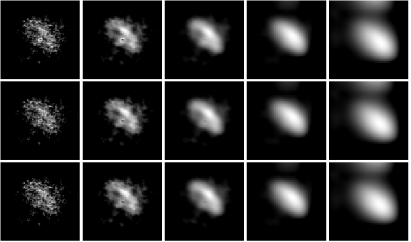
Figure 3: Deconvolved images of the Crab Nebula made from the data of Hitomi HXI-1 in $3.6-15$keV band without the pulsar component, by changing the hyper-parameters ($\log_{10}\mu$, $\log_{10}\gamma$). These values are shown above and to the left of the figure, respectively. The best image determined by the cross-validation is the one at ($-5$, $-9$).

	$3.6-15$keV (HXI-1)       $15-30$ keV (HXI-1,2)       $30-70$keV (HXI-1,2)
Deconvolved                                     Observed

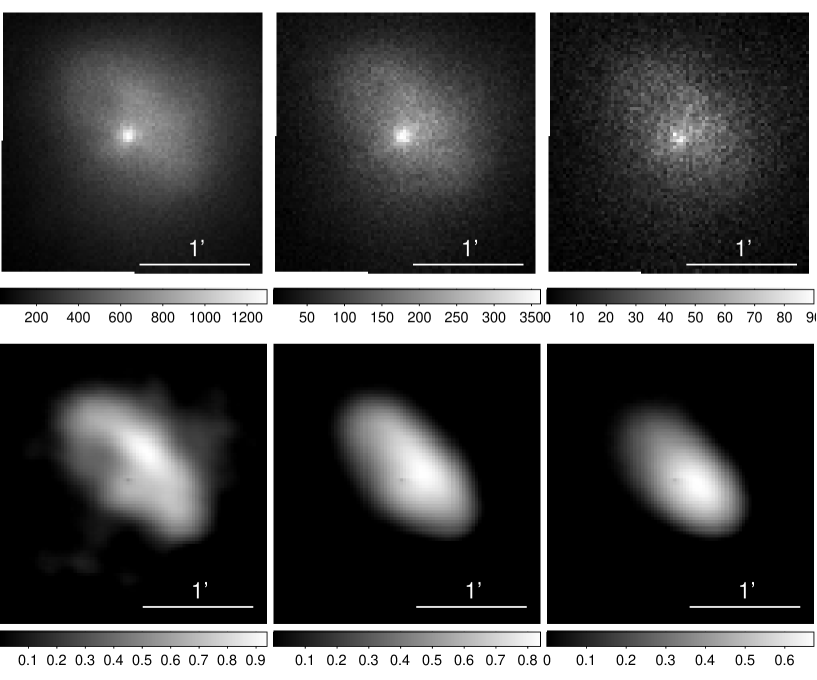
Figure 4: The observed and deconvolved images of the Crab Nebula obtained by Hitomi HXI in three energy bands. The upper and lower panels show the observed images taken by HXI and the deconvolved images without the pulsar component, respectively. The left panels show $3.6-15$ keV band images using HXT-1 data. The center and right panels show $15-30$ keV and $30-70$ keV band images, respectively, where both HXT-1 and HXT-2 data are used. The deconvolved images are the results with the hyper-parameters of $(\log_{10}\mu,\log_{10}\gamma)=(-5,-9)$, $(-4,-8)$ and $(-3,-7)$, from left to right, in which $\mu$ parameters are determined by the one-standard error rule. The size of panel is $80\times 80$ pixels, and the horizontal line segment shows the size of 1 arcmin in each panel.

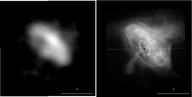
Figure 5: Comparison between the deconvolved Hitomi HXI-1 $3.6-15$ keV band image (left) and Chandra ACIS $0.5-7.0$ keV band image (right). The horizontal line segment shows the size of 1 arcmin in each panel.

We apply the above deconvolution method for the Hitomi observation data for three energy bands of $3.6-15$, $15-30$ and $30-70$ keV. The observed Hitomi HXI images in these energy bands are shown in the upper panels of figure 4. By the cross-validation, we determine the best hyper-parameter and apply the deconvolution with fixing the hyper-parameters. The resultant deconvolved images are shown in the lower panels of figure 4.

As a demonstration of our method, figure 5 shows a comparison between the deconvolved image in $3.6-15$ keV band and Chandra ACIS $0.5-7.0$ keV band image (Mori et al., 2004). Our Hitomi HXI image looks similar with the Chandra image. The torus, south-east jet and north-west extended emission are also seen in our deconvolved image.

13 Evaluation of systematic uncertainty of the response matrix

The response matrix used is expected to contain the following three kinds of uncertainties. We evaluate the effects for the deconvolved image.

13.1 Uncertainty of livetime fraction

Table 4 shows the livetime fraction for each phase, calculated by the method in the appendix of Matsumoto et al. (2018). It confirms that the livetime fraction at each phase is about three-fourths, and that the ON phase image has less livetime fraction than the OFF, because the phase of higher count rate has the lower livetime fraction. Matsumoto et al. (2018) also reported that the uncertainty on the deadtime fraction ($F_{\rm dt}$) at the 1$\sigma$ confidence level is $\Delta F_{\rm dt}/F_{\rm dt}=2$%. So, the uncertainty of the livetime fraction ($F_{\rm lt}$) is $\Delta F_{\rm lt}/F_{\rm lt}=(F_{\rm dt}/F_{\rm lt})\times(\Delta F_{\rm dt}/F_{\rm dt})\sim(0.25/0.75)\times 2\%=0.7\%$.

Table 4: Livetime fraction of each pulse phase ID

Phase ID	Phase	Phase duration	Livetime fraction
			HXI-1	HXI-2
All	0-1	1	0.766	0.752
ON2	0.854-1.104	0.25	0.750	0.735
OFF1	0.104-0.504	0.40	0.783	0.770
ON1	0.504-0.704	0.20	0.747	0.731
OFF2	0.704-0.854	0.15	0.773	0.758

Since the PSF is made by the image subtraction of ON minus OFF1 pulse phase, the uncertainty of the livetime fraction causes the uncertainty for the shape of the subtracted image. In order to evaluate the effect of the uncertainty for the deconvolved image conservatively, we increase/decrease the livetime of OFF1 image by $2$%, corresponding to $3\times\sim 0.7$%, make the PSF by the ON-OFF1 operation, and deconvolve the Crab Nebula image in the 3.6-15 keV band. Figure 6 shows the deconvolved images made by using the response matrices in three different livetime cases. There are no significant difference among these images. We then conclude that the livetime uncertainty does not affect the deconvolved images.

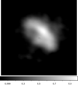
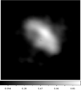
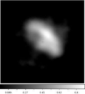
Figure 6: The deconvolved images of the Crab Nebula in the 3.6–15 keV band, using three different response matrices, made by assuming different livetime fraction for the OFF1 image. Here, the cases of 2% decrease, nominal and 2% increase of the livetime fraction are shown in left, center and right panels, respectively.

13.2 Uncertainty of optical axis location

The HXT shows a sharp vignetting effect as reported in Awaki et al. (2014). They showed that the effective area decreases by 10–20% (dependent on energy) at 1 arcmin off-axis from the optical axis. Therefore, the uncertainty of the optical axis location can affect the shape of the deconvolved image. By the energy spectral analysis of Matsumoto et al. (2018) and Hagino et al. (2018), the location of the Crab pulsar is confirmed to be within 0.5 arcmin from the optical axis. We thus evaluate the difference of the deconvolved images made by changing the exposure maps corresponding to the different optical axis locations, within the conservative uncertainty of 1 arcmin from the pulsar position.

We make the exposure maps assuming three different optical axis locations using the ray-tracing code xrrtraytrace (Angelini et al. (2016)) for each energy band. The deconvolved images corrected for these exposure maps are shown in figure 7, where the optical axis is located at 1 arcmin shifted to north-east direction (top row), at the pulsar position (middle row), and 1 arcmin shifted to south-west direction (bottom row). In figure 7, no remarkable difference are seen among different optical axes and these energy bands. Thus, we conclude that the uncertainty of the optical axis location does not affect the deconvolved images.

		Energy band [keV]
		$3.6$–$15$                          $15$–$30$                              $30$–$70$
Position of an assumed optical axis	bottom right                        center                        upper left

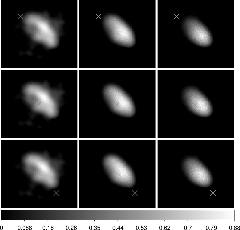
Figure 7: Exposure-corrected deconvolved images in the 3.6–15 (left column), 15–30 (center column) and 30–70 (right column) keV bands for three different optical-axis locations. The cross mark is the optical-axis location we assumed to make the exposure map. The middle row images are deconvolved by assuming the optical axis is located at the pulsar position. In the upper and lower panels, the optical axes are located 1 arcmin to north-east and south-west directions from the pulsar position, respectively.

13.3 Uncertainty of the off-axis PSF

The off-axis effect is known to not only reduce the effective area but also change the PSF (Awaki et al., 2014). Since the drop of the effective area at 1 arcmin off-axis location is only 10-20%, it contributes small change of the PSF. It is also known that the conical approximation adapted for the HXT shows negligible off-axis dependence of the HPD of the PSF (Petre et al., 1985). Thus, we decide to adapt the Crab pulsar PSF to all in-coming directions in this paper.

14 Image analysis

As shown in figure 4, the nebula size is obviously smaller in higher energy bands. In order to measure the nebula size, we project the image along the minor and major axes as shown in figure 8 (left), which are rotated clockwise by 54 degrees from the north and west directions, respectively. Here, the minor axis is determined to align the pulsar spin axis obtained by the Chandra image. The projected images in these axes are shown in figure 8 (center and right). The nebula sizes in these axes are listed in table 5. They clarify such the trend that the nebula is smaller in higher energy bands. Here, we need mention that the higher energy bands have smaller number of photons, then the smoothing parameter ($\mu$) tends to be large, and so the resulting nebula image tends to be large. Nevertheless, the harder band images show smaller nebula size. Thus, this trend is strongly supported. It was also pointed out by the NuSTAR using the OFF1 phase data (Madsen et al., 2015).

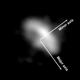
Figure 8: Projections of the deconvolved images along the minor and major axes (center and right, respectively), whose axes are shown in the left image (3.6-15 keV band). The origins are at the pulsar position. The solid, dash and dash-dot lines correspond to the energy bands of 3.6–15, 15–30 and 30–70 keV, respectively. The peaks are normalized by unity.

Table 5: Nebula size evaluated by FWHM in three energy bands

Energy band	Minor axis	Major axis
keV–keV	Pixels (arcsec)	Pixels (arcsec)
3.6–15	22(39)	41(72)
15–30	20(35)	36(64)
30–70	19(34)	30(53)

Along the minor axis, the north-west (NW) direction is brighter than the south-east (SE) direction in all energy bands. It is explained by the relativistic viewing effect of the high energy electron/positron at the torus (Mori et al. (2004) and reference therein). Along the major axis, the north-east (NE) direction is darker than the south-west (SW) direction in higher energy band. This trend is reported for the first time.

15 Discussion and future perspective

Our deconvolution image of the Hitomi HXI in the 3.6–15 keV band succeeds to clarify the torus-like structure including its inner boundary. The structure does not appear in the deconvolved image of the NuSTAR data using the Richardson-Lucy method (Madsen et al., 2015). Both NuSTAR and Hitomi have nearly equal angular resolution in HPD. So, the difference is thought to be caused by two advantages in our work. The first one is our ingenious method that introduces two components for the nebula and pulsar with regularization for smoothness and flux, respectively, and the multi-pulse-phase simultaneous deconvolution. The second one is the sharp core of the PSF of the Hitomi HXT, which is smaller by a factor of two than that of NuSTAR. It simply improves the angular resolution of the deconvolved image.

We can not clearly identify the torus-like structure in the hard X-ray image using the same method above 15 keV. We however confirm the NuSTAR’s findings that the size of the Crab Nebula decreases in higher energy bands. Madsen et al. (2015) pointed out the discrepancy of the averaged photon index of the nebula: $\sim 1.9$ (Mori et al., 2004) and $\sim 2.140\pm 0.001$ above 100 keV (Pravdo, Angelini, and Harding, 1997). They also pointed out that the discrepancy is due to the spectral cut-off of the outer torus around the 10–100 keV band. Using the Hitomi data, we found that the north-east becomes darker in the higher energy bands, indicating the spectra of the north-east torus is more rapidly cut off than that of the south-west. We expect our result will promote the theoretical works of the Crab Nebula.

Our deconvolution algorithm can be applicable for any telescope images of faint diffuse objects containing a bright point source, and effectively works especially for the case that the apparent size of the diffuse objects is comparable with that of the PSF of the telescope. We also mention that the algorithm can be extended for objects with multiple point sources. Another extension would be possible to introduce smoothness constraint for the energy direction. The calculation speed would be improved by more tuning in the CUDA coding. It is also improved by introducing some acceleration methods of the MM algorithm. Indeed, we observed the decrease of the number of iterations by the acceleration methods (Varadhan and Roland, 2008; Zhou, Alexander, and Lange, 2011). For the hyper-parameter tuning, the Bayesian optimization is a promising method (Garnett, 2023). We make our source code open for public use .

This research is supported by JSPS Grants-in-Aid for Scientific Research (KAKENHI) Grants No. 22H01277 and 21H01095.

Appendix A Detailed calculation

The surrogate function for $V(I)$ function is

$$u(I;I^{\prime}) = \frac{1}{2}\sum_{(r,s)\in N}\{[2I_{r}-(I_{r}^{\prime}+I_{s}^{\prime})]^{2}+[2I_{s}-(I_{r}^{\prime}+I_{s}^{\prime})]^{2}\}$$ (41)

$$= \frac{1}{2}\left(\sum_{i=1}^{m-1}\sum_{j=1}^{n-1}\{[2I_{i,j}-(I_{i,j}^{\prime}+I_{i+1,j}^{\prime})]^{2}+[2I_{i+1,j}-(I_{i,j}^{\prime}+I_{i+1,j}^{\prime})]^{2}\right.$$

$$+[2I_{i,j}-(I_{i,j}^{\prime}+I_{i,j+1}^{\prime})]^{2}+[2I_{i,j+1}-(I_{i,j}^{\prime}+I_{i,j+1}^{\prime})]^{2}\}$$

$$+\sum_{i=1}^{m-1}\{[2I_{i,n}-(I_{i,n}^{\prime}+I_{i+1,n}^{\prime})]^{2}+[2I_{i+1,n}-(I_{i,n}^{\prime}+I_{i+1,n}^{\prime})]^{2}\}$$

$$\left.+\sum_{j=1}^{n-1}\{[2I_{m,j}-(I_{m,j}^{\prime}+I_{m,j+1}^{\prime})]^{2}+[2I_{m,j+1}-(I_{m,j}^{\prime}+I_{m,j+1}^{\prime})]^{2}\}\right)$$

and the derivative of $u(I;I^{\prime})$ is

$$\frac{\partial u(I;I^{\prime})}{\partial I_{kl}} = \frac{1}{2}\left(\sum_{i=1}^{m-1}\sum_{j=1}^{n-1}\{2[2I_{i,j}-(I_{i,j}^{\prime}+I_{i+1,j}^{\prime})]2\delta_{i,k}\delta_{j,l}+2[2I_{i+1,j}-(I_{i,j}^{\prime}+I_{i+1,j}^{\prime})]2\delta_{i+1,k}\delta_{j,l}\right.$$ (42)

$$+2[2I_{i,j}-(I_{i,j}^{\prime}+I_{i,j+1}^{\prime})]2\delta_{i,k}\delta_{j,l}+2[2I_{i,j+1}-(I_{i,j}^{\prime}+I_{i,j+1}^{\prime})]2\delta_{i,k}\delta_{j+1,l}\}$$

$$+\sum_{i=1}^{m-1}\{2[2I_{i,n}-(I_{i,n}^{\prime}+I_{i+1,n}^{\prime})]2\delta_{i,k}\delta_{n,l}+2[2I_{i+1,n}-(I_{i,n}^{\prime}+I_{i+1,n}^{\prime})]2\delta_{i+1,k}\delta_{n,l}\}$$

$$\left.+\sum_{j=1}^{n-1}\{2[2I_{m,j}-(I_{m,j}^{\prime}+I_{m,j+1}^{\prime})]2\delta_{m,k}\delta_{j,l}+2[2I_{m,j+1}-(I_{m,j}^{\prime}+I_{m,j+1}^{\prime})]2\delta_{m,k}\delta_{j+1,l}\}\right)$$

$$= ({\rm term1})+({\rm term2})+({\rm term3})+({\rm term4})$$

$$+({\rm term5})+({\rm term6})+({\rm term7})+({\rm term8}).$$

Here,

$$({\rm term1}) = \left\{\begin{array}[]{cc}2[2I_{k,l}-(I_{k,l}^{\prime}+I_{k+1,l}^{\prime})]&(1\leq k\leq m-1,1\leq l\leq n-1)\\ 0&({\rm otherwise})\end{array}\right.,$$ (45)

$$({\rm term2}) = \left\{\begin{array}[]{cc}2[2I_{k,l}-(I_{k-1,l}^{\prime}+I_{k,l}^{\prime})]&(2\leq k\leq m,1\leq l\leq n-1)\\ 0&({\rm otherwise})\end{array}\right.,$$ (48)

$$({\rm term3}) = \left\{\begin{array}[]{cc}2[2I_{k,l}-(I_{k,l}^{\prime}+I_{k,l+1}^{\prime})]&(1\leq k\leq m-1,1\leq l\leq n-1)\\ 0&({\rm otherwise})\end{array}\right.,$$ (51)

$$({\rm term4}) = \left\{\begin{array}[]{cc}2[2I_{k,l}-(I_{k,l-1}^{\prime}+I_{k,l}^{\prime})]&(1\leq k\leq m-1,2\leq l\leq n)\\ 0&({\rm otherwise})\end{array}\right.,$$ (54)

$$({\rm term5}) = \left\{\begin{array}[]{cc}2[2I_{k,n}-(I_{k,n}^{\prime}+I_{k+1,n}^{\prime})]&(1\leq k\leq m-1,l=n)\\ 0&({\rm otherwise})\end{array}\right.,$$ (57)

$$({\rm term6}) = \left\{\begin{array}[]{cc}2[2I_{k,n}-(I_{k-1,n}^{\prime}+I_{k,n}^{\prime})]&(2\leq k\leq m,l=n)\\ 0&({\rm otherwise})\end{array}\right.,$$ (60)

$$({\rm term7}) = \left\{\begin{array}[]{cc}2[2I_{m,l}-(I_{m,l}^{\prime}+I_{m,l+1}^{\prime})]&(k=m,1\leq l\leq n-1)\\ 0&({\rm otherwise})\end{array}\right.,$$ (63)

$$({\rm term8}) = \left\{\begin{array}[]{cc}2[2I_{m,l}-(I_{m,l-1}^{\prime}+I_{m,l}^{\prime})]&(k=m,2\leq l\leq n)\\ 0&({\rm otherwise})\end{array}\right..$$ (66)

Appendix B Proof of convergence of our algorithm

Here, we proof convergence of our algorithm, partly following the proof shown in Kanamori et al. (2016). The cost function $L_{\rm cost}(x)$ is defined at a non-negative orthant, where $x=(I,f)\in\{x\in R^{M+n_{p}}|x_{i}\geq 0\,\,(i=1,2,\cdots,M+n_{p})\}$. It is a continuous proper convex function, and then closed [Rockafellar (1970), section 7]. It becomes infinity when $|x|\rightarrow\infty$, then it has no directions of recession [Rockafellar (1970), section 8]. Because of Rockafellar (1970), Theorem 27.1 (d), the minimum set of $L_{\rm cost}$ is a non-empty bounded closed convex set. All the level set ${\rm lev}_{\alpha}L_{\rm cost}=\{x\in R^{M+n_{p}}|L_{\rm cost}(x)\leq\alpha\}$ ($\alpha\in{\rm R}$) is a bounded closed convex set [Rockafellar (1970), Theorem 27.1 (f) and Theorem 8.4], and then a compact set. Since $\mu V(I)+\gamma D(f)$ is strictly convex and $-\log p(Y|I,f)$ is convex, $L_{\rm cost}(x)$ is also a strictly convex function in any level set [Rockafellar (1970), section 26]. So, the minimum set of $L_{\rm cost}$ cannot contain more than one point [Rockafellar (1970), Section 27], then the minimum set of $L_{\rm cost}$ is made up of a unique point.

The MM algorithm produce a sequence $(x^{(r)})_{r=1,2,\cdots}$ from any feasible initial value $x^{(0)}$ such that $L_{\rm cost}(x^{(0)})$ is finite. Since the level set ${\rm lev}_{\rm init}=\{x\in R^{M+n_{p}}|L_{\rm cost}(x)\leq L_{\rm cost}(x^{(0)})\}$ is a compact set, there exists a sub-sequence $(x^{(r_{k})})_{k=1,2,\cdots}$ which converges to a value within the level set: $\lim_{k\rightarrow\infty}x^{(r_{k})}=x^{*}\in{\rm lev}_{\rm init}$. Since the MM algorithm produces a monotonically decreasing sequence: $L_{\rm cost}(x^{(r)})\geq L_{\rm cost}(x^{(s)})\,\,(r<s)$, $u_{\rm cost}(x^{(r_{k+1})};x^{(r_{k+1})})=L_{\rm cost}(x^{(r_{k+1})})\leq L_{\rm cost}(x^{(r_{k}+1)})\leq u_{\rm cost}(x^{(r_{k}+1)};x^{(r_{k})})\leq u_{\rm cost}(x;x^{(r_{k})})$ for any $x\in{\rm lev}_{\rm init}$. When $k\rightarrow\infty$, $u_{\rm cost}(x^{*};x^{*})\leq u_{\rm cost}(x;x^{*})$. Since $u_{\rm cost}(x;x^{*})$ is a differentiable convex function on $x$, $0\in\partial u_{\rm cost}(x^{*};x^{*})=\{\nabla u_{\rm cost}(x^{*};x^{*})\}$. Then, $\nabla L_{\rm cost}(x^{*})=\nabla u_{\rm cost}(x^{*};x^{*})=0$. Thus, $x^{*}$ is the unique point in the minimum set of $L_{\rm cost}$. So, $(x^{(r_{k})})_{k=1,2,\cdots}$ is a sequence such that $(L_{\rm cost}(x^{(r_{k})}))_{k=1,2,\cdots}$ converges to $\inf L_{\rm cost}$. Because of the monotonicity of the MM sequence, $(L_{\rm cost}(x^{(r)}))_{r=1,2,\cdots}$ also converges to $\inf L_{\rm cost}$. Thus, the MM sequence $(x^{(r)})_{r=1,2,\cdots}$ converges to the unique minimum point $x^{*}$ [Rockafellar (1970), Corollary 27.2.2].

References

- Angelini et al. (2016) Angelini, L., et al. 2016, Proc. SPIE, 9905, 990514
- Awaki et al. (2014) Awaki, H., et al. 2014, Appl. Opt., 53, 7664
- Bishop (2006) Bishop, C. M. 2006, Pattern Recognition and Machine Learning (New York: Springer New York)
- Dempster, Laird, and Rubin (1977) Dempster, A. P., Laird, N. M., & Rubin, D. B. 1977, Journal of the Royal Statistical Society, Series B (Methodological), 39, 1
- Ducros et al. (1970) Ducros, G., Ducros, R., Rocchia, R., & Tarrius, A. 1970, Nature, 227, 152
- Garnett (2023) Garnett, R. 2023, Bayesian Optimization (Cambridge, UK: Cambridge University Press)
- Hagino et al. (2018) Hagino, K., et al. 2018, Journal of Astronomical Telescopes, Instruments, and Systems, 4, 021409
- Harrison et al. (2013) Harrison, F. A., et al. 2013, ApJ, 770, 103
- Hastie, Tibshirani, and Wainwright (2015) Hastie, T., Tibshirani, R., & Wainwright, M. 2015, Statistical Learning with Sparsity: The Lasso and Generalizations (London: Routledge)
- Hitomi Collaboration et al. (2018) Hitomi Collaboration, et al. 2018, PASJ, 70, 15
- Hunter and Lange (2000) Hunter, D. R., & Lange, K. 2000, Journal of Computational and Graphical Statistics, 9, 60
- Kanamori et al. (2016) Kanamori, T., et al. 2016, Continuous optimization for machine learning, (Tokyo: Kohdansha) (written in Japanease)
- Kennel and Coroniti (1984) Kennel, C. F., & Coroniti, F. V. 1984, ApJ, 283, 694
- Lucy (1974) Lucy, L. B. 1974, AJ, 79, 745
- Madsen et al. (2015) Madsen, K. K., et al. 2015, ApJ, 801, 66
- Matsumoto et al. (2018) Matsumoto, H., et al. 2018, Journal of Astronomical Telescopes, Instruments, and Systems, 4, 011212
- Mori et al. (2004) Mori, K., Burrows, D. N., Hester, J. J., Pavlov, G. G., Shibata, S., & Tsunemi, H. 2004, ApJ, 609, 186
- Morii, Ikeda, and Maeda (2019) Morii, M., Ikeda, S., & Maeda, Y. 2019, PASJ, 71, 24
- Nakazawa et al. (2018) Nakazawa, K., et al. 2018, Journal of Astronomical Telescopes, Instruments, and Systems, 4, 021410
- Rees and Gunn (1974) Rees, M. J., & Gunn, J. E. 1974, MNRAS, 167, 1
- Petre et al. (1985) Petre, R., & Serlemitsos, P. J. 1985, Appl. Opt., 24, 1833
- Porth, Komissarov, and Keppens (2014) Porth, O., Komissarov, S. S., & Keppens, R. 2014, MNRAS, 438, 278
- Pravdo, Angelini, and Harding (1997) Pravdo, S. H., Angelini, L., & Harding, A. K. 1997, ApJ, 491, 808
- Richardson (1972) Richardson, W. H. 1972, Journal of the Optical Society of America, 62, 55
- Rockafellar (1970) Rockafellar, R. T. 1970, Convex Analysis (Princeton, New Jersey: Princeton University Press)
- Takahashi et al. (2016) Takahashi, T., et al. 2016, Proc. SPIE, 9905, 99050U
- Varadhan and Roland (2008) Varadhan R., & Roland, C. 2008 Scandinavian Journal of Statistics, 35, 335
- Weisskopf et al. (2000) Weisskopf, M. C., et al. 2000, ApJ, 536, L81
- Zhou, Alexander, and Lange (2011) Zhou, H., Alexander, D., & Lange, K. 2011, Statistics and Computing, 21, 261